Finite Time ESO-Based Line-of-Sight Following Method with Multi-Objective Path Planning Applied on an Autonomous Marine Surface Vehicle

Abstract

The multi-objective path planning and robust continuous path-following method for the autonomous marine surface vehicle (AMSV) is employed. By incorporating the position and direction constraints into the optimization cost function, the spiral path planner obtains a continuous path with smooth path tangency and curvature and ensures strict adherence to the desired multi-objective points. An improved A* and optimization algorithm are combined with the global path planning to avoid obstacles in real-time. For the path-following controller, the unknown sideslip angle and uncertainties are added to build the system model, based on which observation technique is adopted to estimate all the uncertainties online. Based on the kinematic system, a finite time extended state observer (ESO) is put forward to estimate the sideslip angle accurately. The nonlinear line-of-sight (LOS) guidance scheme is designed for the model, effectively compensating for the observed values and achieving convergence in a finite time. The finite-time ESO is adopted to estimate the uncertainty for the surge and heading controller design, and the terminal sliding mode technique is introduced to achieve the final finite-time convergence. Through extensive experiments, the proposed approach demonstrates its effectiveness, feasibility, and the advantage of fast convergence and accurate control.

1. Introduction

Many path-planning and path-following methods of the autonomous driving system (ADS) have been developed for the under-actuated-based marine surface vehicle (MSV). For the AMSV, having a continuous reference path that can achieve smooth control without overshooting is essential [1]. The AMSV needs to pass through each intermediate point precisely in the multiple-objective navigation path (MONP), where the multi-objective refers to the intermediate points (including position and orientation) that are used to generate the global path. A simple way to plan a MONP is to connect all the objective waypoints with straight lines, but this causes discontinuity in the path-tangential angle at the junctions, which may lead to cross-track error or instability. To solve this problem, the Dubins proposed a path generator that uses straight lines and inscribed circle arcs [2]. However, this method still has a discontinuity in the curvature, which causes a sudden change in the desired yaw angle velocity at straight line and circle arc transitions. In [3], a cubic Hermite spline-based path planner algorithm was developed to generate a smooth path, but it cannot exactly pass through the target waypoint. To pass through all the objective points smoothly, especially when facing obstacles, the optimization scheme based on the critical constraints was mentioned in [4]. The kinematic controller uses the guidance law (GDL) to follow the reference path in this method. Then, the dynamics controller uses the GDL to make the vehicle track the command velocity and course angle. LOS-GDL was first introduced in [5] and has been widely used in vehicle path-following control [6]. These methods assume that the sideslip angle is measurable, but in practice, it should be calculated by the sway speed. To improve system performance, the integral LOS and adaptive LOS [7] are used to deal with the drift force and wave disturbance, but the stability characteristics of the guidance system still need further study. The active disturbance rejection control (ADRC) was first mentioned in [8] and has been extensively applied in practical applications [9]. The ESO, which is the essential part of ADRC, can estimate the system’s unmeasured state and total disturbance and form the corresponding feedback controller [10]. In [11], the unknown nonlinear function with sideslip angle was reconstructed as a system state, and then ESO was used to estimate and compensate for this unknown nonlinear term in the GDL. The extended state of this method also contains a known nonlinear factor, which increases the uncertainty to be estimated and limits the bandwidth of the ESO.

After planning the global path, a local path modifier method must be considered to adjust the global path according to the dynamic environment and the obstacle motion [12]. It involves detecting and avoiding potential collisions with other vessels or static obstacles in a dynamic environment while complying with the rules and regulations of navigation. The authors of [13] proposed an automatic MSV control system that can navigate and steer in a narrow environment using the camera, radar, ultrasound, and a deep learning-based segmentation method. This method can identify the area where the vessel can sail safely. The system also used an MPC-based algorithm to generate and follow a collision-free real-time path. An improved A-star algorithm and an improved dynamic window method for MSV path planning and collision avoidance in crowded and highly uncertain sea areas were proposed by [14]. These methods enabled the vessel to sail autonomously by planning and updating the real-time path and avoiding obstacles effectively. Using a partial minimum consensus method in a layered structure, the MSV navigation system in [15] could navigate quickly to the target point while avoiding and distancing from obstacles. Meanwhile, ocean current interference was only considered in path planning, ignoring its influence on the control stage, resulting in a discontinuous curvature scene of the planned path, which affects path-following accuracy. By combining global and local path planning in [16], discrete optimal paths were generated globally, surge and yaw velocity were generated locally according to fuzzy decision-making and precisely adjusted dynamic window modules, which could generate the shortest path and handle some unknown and uncertain scenes. However, this scheme did not consider the intermediate point constraint during planning, it is unsuitable for continuous navigation between multi-objective paths. Besides, this method based on accurate adjustment of dynamic windows would be easy to fall into local optimal in complex scenes, affecting the navigation efficiency. Ref. [17] introduced a Gaussian process motion planning 2-star controller that can handle complex environments with multiple environmental characteristics, such as the ocean. This controller extended the essential motion planning based on the Gaussian process, which only works for environments with obstacles. In [18], obstacle information was directly put into the model-free reinforcement learning control, which avoided complex modeling by optimizing the physical constraints of the AMSV itself and simultaneously greatly reduced the amount of computation. However, the generated path did not consider the influence of obstacles, and the path following based on reinforcement learning requires a large amount of training data and did not involve the changes in the external environment (ocean currents) and internal factors (such as mass).

Various vehicle motion control algorithms based on the GDL have been proposed to make the AMSV track the command velocity and course angle. The neural network algorithm was used to estimate the uncertainties [19] but is hard to apply in practice due to the high dependence on initial values. The backstepping algorithm was used [20,21] but could not achieve finite-time convergence. In [22,23], the sliding mode control (SMC) method was used to design the motion controller, but it suffered from the chattering phenomenon. To overcome this problem, a high-order SMC was proposed [24,25] to sacrifice the high calculation burden. An adaptive robust control method was used to improve the control performance under uncertainties [26]; however, it is very conservative. Recently, the disturbance–observer (DOB)-based method has been studied extensively in the motion controller design to enhance robustness and performance [27].

The multi-objective following task solved here involves path planning and robust controller design. The path planner generates a smooth path that can pass through all the objective waypoints. When obstacles exist, the real-time obstacle avoidance planning algorithm will generate paths that avoid the obstacles based on the orientation of these intermediate points to ensure that the AMSV can reach the target position safely and stably. The robust controller reduces or eliminates the effects of nonlinearity, strong coupling, and uncertainties.

The main contributions are summarized as follows:

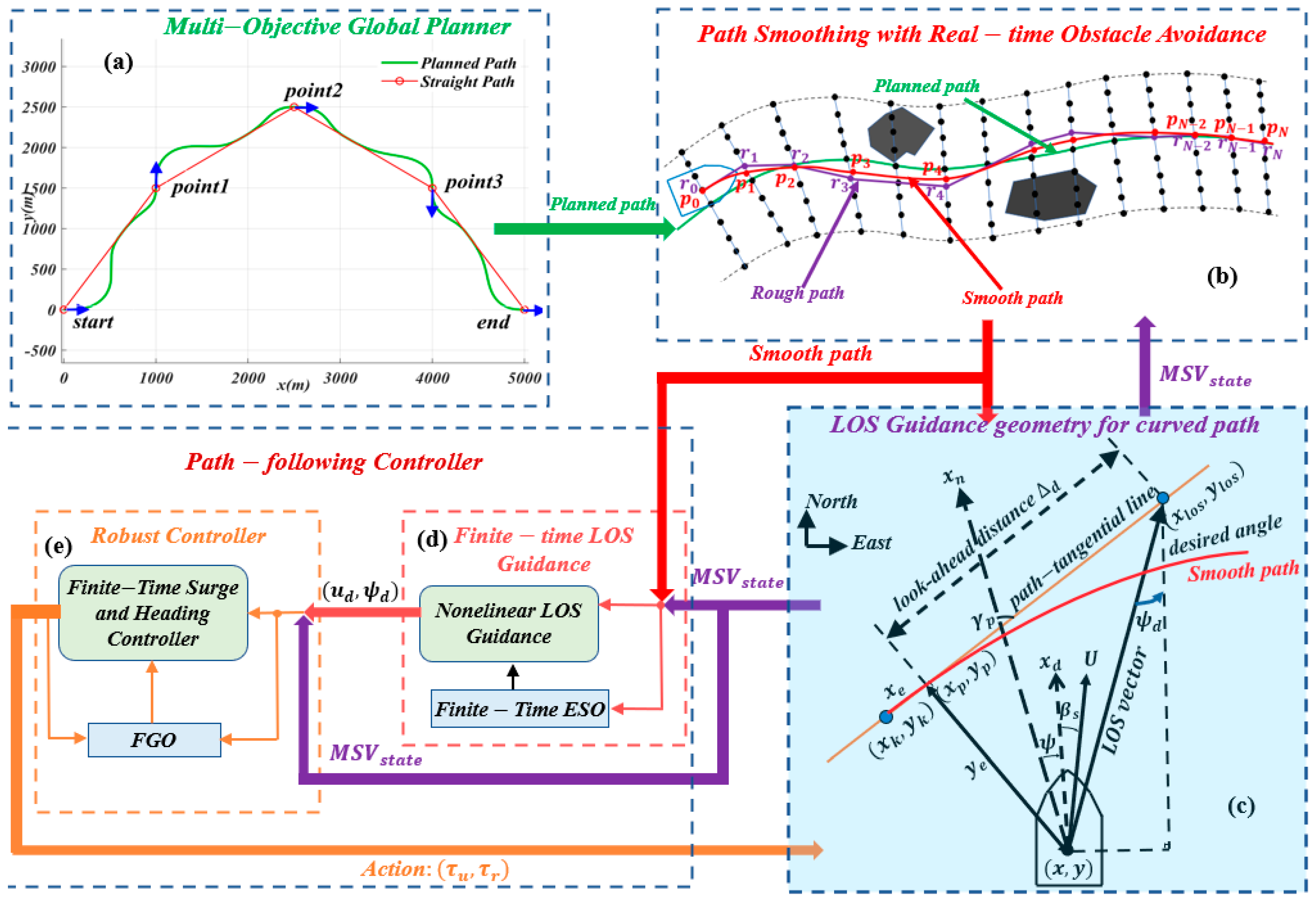
• A multi-objective spiral programming algorithm generates a continuous and sequential path that passes through all target points.
• An improved A* algorithm and an optimization algorithm are combined to perform global path planning and timely obstacle avoidance near the path.
• A finite-time ESO is constructed to estimate the time-varying unknown sideslip angle and a nonlinear feedback LOS-GDL is built to achieve finite-time convergence.
• A terminal sliding mode and a nonlinear DOB are used to build a surge course finite-time controller.

The problem description and MSV model are given in Section 2. Section 3 presents a multi-objective spiral path planner and path smoothing. Section 4 introduces a finite-time ESO to estimate the unknown and time-varying sideslip angle and uses a nonlinear feedback LOS-GDL to achieve finite-time convergence. Section 5 designs a finite-time surge and heading controller. Section 6 gives the results and its analysis. Section 7 concludes the proposed work.

2. System Statement

2.1. Problem Formulation

Figure 1 illustrates the framework of the AMSV system, while Figure 2 shows the structure of the proposed method. By integrating these two figures, we can provide a detailed description of the entire control system as follows:

(1). In the Multi-Objective Global Planner shown in Figure 1a, a smooth reference path that goes through all the target points without overshooting so that the AMSV can follow the path accurately;

(2). In Figure 1b, the obstacle avoidance algorithm that uses global path planning with improved A* and optimization to avoid obstacles near the route in time;

(3). A path-following controller that consists of the LOS guidance algorithm for horizontal kinematics is shown in Figure 1d, and a robust motion controller is given in Figure 1e for surge and heading kinematics, which stabilizes the error system and makes the AMSV track the reference path quickly and precisely.

(4). Figure 1c shows the geometric relationship between LOS-GDL and the expected track based on forward-looking distance. The current position coordinate is defined as $(x,y)$ and the pedal point as $(x_p,y_p)$; thus, $y_e$ is the orthogonal disturbance from the current location to $(x_p,y_p)$ and similarly to the longitudinal error $x_e$.

Since this method is designed for multi-target paths, the kinematic constraints of the AMSV must be followed at each intermediate point, which significantly increases the amount of computation as the number of target points increases. However, for the autonomous driving process, the global path planning algorithm can be calculated offline, so it will not have a big impact on the actual performance of autonomous driving. In addition, the local obstacle avoidance path of this solution generated by Figure 1b adopts real-time planning.

The path-tangential angle ${\gamma }_p$ and the cross-track error $y_e$ can be obtained according to the waypoints of the reference path, while the sideslip angle ${\beta }_s$ is usually unmeasured. ${\beta }_s$ is caused by drift forces, which is usually less than $5°$, but it affects the path-following control for the AMSV and needs to be estimated and compensated in the guidance algorithm. And its time-derivative ${\dot{\beta }}_s$ is obtained in (1), where $v_{su}$, $v_{sw}$ are the speed of surge and sway. Obviously, ${\beta }_s$ and ${\dot{\beta }}_s$ are bounded and defined as: $\left|{\beta }_s\right|\le {\beta }_1,|{\dot{\beta }}_s|\le {\beta }_2$.

$${\dot{\beta }}_s={\displaystyle \frac{{\dot{v}}_{sw}{v}_{su}-{\dot{v}}_{su}{v}_{sw}}{{v_{su}}^2+{v_{sw}}^2}}$$

(1)

2.2. Description of the AMSV Model

The 3-DOF kinematics of the AMSV is presented in (2) based on the paper [28], where $\psi$, and $v_{ya}$ represent the yaw angle and the yaw speed.

$$\left\{\begin{array}{c}\dot{x}=v_{su}\cos \psi -v_{sw}\sin \psi \\ \dot{y}=v_{su}\sin \psi +v_{sw}\cos \psi \\ \dot{\psi }=v_{ya}\end{array}\right.$$

(2)

Assume that the rotation angle of the path tangent reference system is ${\gamma }_p$, then the trajectory tangent reference system can be described by ${\gamma }_p$ and the rotation matrix $R\left({\gamma }_p\right)$ [29]. By rotating ${\gamma }_p$, and using the attitude transition matrix $R\left({\gamma }_p\right)$, $x_e$ and $y_e$ are given in (3).

$$\left\{\begin{array}{c}\left[\begin{array}{c}{x}_e\\ y_e\end{array}\right]={R\left({\gamma }_p\right)}^T\left[\begin{array}{c}x-x_p\\ y-y_p\end{array}\right]\\ {R\left({\gamma }_p\right)}^T=\left[\begin{array}{cc}\cos \left({\gamma }_p\right)& -\sin \left({\gamma }_p\right)\\ \sin \left({\gamma }_p\right)& \cos \left({\gamma }_p\right)\end{array}\right]\end{array}\right.$$

(3)

$$\left\{\begin{array}{c}{\dot{x}}_e=v\cos \left(\psi -{\gamma }_p+{\beta }_s\right)+{\dot{\gamma }}_p{y}_e-v_{su}\\ {\dot{y}}_e=v\sin \left(\psi -{\gamma }_p+{\beta }_s\right)-{\dot{\gamma }}_p{y}_e\end{array}\right.$$

(4)

According to (3), the first-order time derivative of $x_e$ and $y_e$ can be given. Considering that the sideslip angles caused by the drift effect are small (<5°), ${\dot{x}}_e$ and ${\dot{y}}_e$ can be approximated by trigonometric functions and are shown in (4), where the amplitude $v=\sqrt{{v_{su}}^2+{v_{sw}}^2}>0$ and the phase ${\beta }_s=\arctan (v_{sw},v_{su})$ are the speed and sideslip angle, respectively.

The 3-DOF AMSV dynamics is given in (5), where $m_{ii}$ and $d_{ii},(i=\mathrm{1,2},3)$ denote the nominal values of the AMSV inertial and damping, ${\tau }_{su}$ and ${\tau }_{ya}$ stand for the surge force and yaw moment, respectively. ${\tau }_{\mathrm{i}},(i=\mathrm{1,2},3)$ is the total disturbances of the three axes. $v_{su}=v\cos \left({\widehat{\beta }}_s\right)$ and $v_{sw}=v\sin \left({\widehat{\beta }}_s\right)$ are used, where ${\widehat{\beta }}_s$ denotes the estimation of ${\beta }_s$.

$$\left\{\begin{array}{c}{m}_{11}{\dot{v}}_{su}=m_{22}{v}_{sw}{v}_{ya}-d_{11}{v}_{su}+{\tau }_{su}+{\tau }_1\\ m_{22}{\dot{v}}_{sw}=m_{22}{v}_{su}{v}_{ya}-d_{22}{v}_{sw}+{\tau }_2\\ m_{33}{\dot{v}}_{ya}=\left(m_{11}-m_{22}\right)v_{su}{v}_{sw}-d_{33}{v}_{ya}+{\tau }_{ya}+{\tau }_3\end{array}\right.$$

(5)

3. Path Planning and Smoothing

3.1. Spiral Path Planner

The proposed method for the LOS guidance algorithm assumes that the AMSV can follow a reference path perfectly with ${\dot{y}}_e=0$ and $y_e=0$, which implies (6). When there exists $y_e$ and yaw angle tracking error $\tilde{\psi }=\psi -{\psi }_d$, by substituting the control output ${\psi }_d$ of the proposed GDL in Section 4.2, (7) is obtained, where ${\tilde{\beta }}_s={\beta }_s-{\widehat{\beta }}_s$ is the estimation error of ${\beta }_s$, and ${\Delta }_L$ is the look-ahead distance, ${sign}^{\varrho }\left(x\right)=x\cdot {\left|x\right|}^{\varrho -1}$ [30]. As ${\beta }_s$ is relatively small, thus, if $y_e$, $\tilde{\psi }$ and ${\tilde{\beta }}_s$ are bounded, $\psi -{\gamma }_p$ is also bounded.

$$\psi -{\gamma }_p=-{\beta }_s$$

(6)

$$\psi -{\gamma }_p={\tan }^{-1}\left(-{\displaystyle \frac{{\mathrm{sign}}^{{\varrho }_1}\left(y_e\right)}{{\Delta }_L}}\right)-{\beta }_s+{\tilde{\beta }}_s+\tilde{\psi }$$

(7)

A spiral path is defined as (8), where $n$ is the order of a spiral path, $s\in (0,s_f)$ and $s_f$ is the length of the path, $\theta$ is the initial position path angle, $\kappa$ and $\gamma$ denote the curvature and orientation of the path, respectively. The state vector is given as $\mathit{p}\left(\mathit{s}\right)=\left[x\left(s\right)y\left(s\right)\theta \left(s\right)\kappa \left(s\right)\right]$, and its parameters can be expressed as $\mathit{q}=[a_0{a}_1\cdots a_n{s}_f]$. The planned path should satisfy these conditions:

$y_e$ should be below a certain threshold, and the path should switch to a continuous mode when the lateral error exceeds that threshold.

The reference path should have the same orientation as the marine vessel near the pedal point so that the initial value of $\tilde{\psi }$ is small enough.

The path should end at the same position and orientation as the target point and have a low curvature near the end.

$$\left\{\begin{array}{c}\kappa \left(s\right)={\sum }_{i=0}^n{a}_i{s}^i,\gamma \left(s\right)={\sum }_{i=0}^n{\displaystyle \frac{a_i}{i+1}}{s}^{i+1}\\ x\left(s\right)={\int }_0^s\cos \left(\theta \right(s\left)\right)\mathrm{ds},y\left(s\right)={\int }_0^s\sin \left(\theta \right(s\left)\right)\mathrm{ds}\end{array}\right.$$

(8)

$$\left\{\begin{array}{c}\min :J\left(\mathit{q}\right)={\displaystyle \frac{1}{2}}{\int }_0^{s_f}{\left[\kappa \left(\mathit{q}\right)\right]}^2\mathrm{ds}\\ \mathrm{c}\mathrm{o}\mathrm{n}\mathrm{s}\mathrm{t}\mathrm{r}\mathrm{a}\mathrm{i}\mathrm{n}\mathrm{t}\mathrm{s}:\mathit{p}\left(0\right)-p_{start}=0,\mathit{p}\left(s_f\right)-p_{end}=0\end{array}\right.$$

(9)

$$|\psi -{\gamma }_p|\le \delta <{\displaystyle \frac{\pi }{2}}$$

(10)

The path planning problem is expressed as the optimization cost function in (9), which considers the start and target point constraints and is a constrained nonlinear convex optimization problem that numerical methods can solve. The first constraint ensures that the $y_e$ is very small. For ${\tilde{\beta }}_s$ and $\tilde{\psi }$, they will be bounded if the desired ESO and dynamics controller can converge asymptotically, with a proper choice of the origin point. As (7) bounded, $\psi -{\gamma }_p$ in (10) is reasonable, which indicates that $\cos (\psi -{\gamma }_p)>0$ and $1<{\displaystyle \frac{1}{\cos (\psi -{\gamma }_p)}}<{\displaystyle \frac{1}{\cos \delta }}$. If the vessel’s course deviates too much from the tracked path, either by being orthogonal or opposite to it, then (10) does not hold. In this case, the path needs to be replanned by generating a smooth curve that starts from the current position and orientation of the vessel.

3.2. Path Smoothing

If $y_e$ is larger than the setting upper bounded, the proposed Algorithm 1 can be applied directly to replan a smooth path without overshot. Thus, $y_e$ can be constrained into an upper bound defined as ${\overline{y}}_e$.

Algorithm 1 Spiral Path Generator
Input:	Target point sequence $(x_i,y_i),i=0~n$, where $i=0$ denotes the current position of the AMSV
Output:	A smooth reference path denoted by $r(x,y)$
1.	Assign target orientation from $1st$ to $n-1th$ target point
2.	for $k=0\to n-1$ do
3.	${\theta }_k=\arctan 2\left(y_{k+1}-y_k,x_{k+1}-x_k\right),{\mathit{p}}_{\mathit{k}}=\left[x_k{y}_k{\theta }_{k}0\right]$
4.	end for
5.	for $k=0\to n-1$ do
6.	Connect ${\mathit{p}}_{\mathit{k}-1}$ and ${\mathit{p}}_{\mathit{k}}$ to acquire a straight line
7.	Calculate the coordinate of ${\mathit{p}}_{\mathit{j}\mathit{o}\mathit{i}\mathit{n}\mathit{t}1}$ according to the yaw error from ${\mathit{p}}_{\mathit{k}}\left\{3\right\}$ to ${\theta }_k$:   ${\mathit{p}}_{\mathit{k}}^{\mathit{j}\mathit{o}\mathit{i}\mathit{n}\mathit{t}1}\left\{\mathrm{1,2}\right\}={\mathit{p}}_{\mathit{k}}\left\{\mathrm{1,2}\right\}+\left[\begin{array}{c}\mathrm{c}\mathrm{o}\mathrm{s}\left({\theta }_k\right)\\ \sin \left({\theta }_k\right)\end{array}\right]\sqrt{K({\mathit{p}}_{\mathit{k}}\left\{3\right\}-{\theta }_k)}$                                 ${\mathit{p}}_{\mathit{k}}^{\mathit{j}\mathit{o}\mathit{i}\mathit{n}\mathit{t}1}\left\{3\right\}={\mathit{p}}_{\mathit{k}}\left\{3\right\},{\mathit{p}}_{\mathit{k}}^{\mathit{j}\mathit{o}\mathit{i}\mathit{n}\mathit{t}1}\left\{4\right\}=0$
8.	Generate spiral path ${\mathit{q}}_0$ from ${\mathit{p}}_{\mathit{s}\mathit{t}\mathit{a}\mathit{r}\mathit{t}}$ to ${\mathit{p}}_{\mathit{k}}^{\mathit{j}\mathit{o}\mathit{i}\mathit{n}\mathit{t}1}$
9.	Calculate the coordinate of ${\mathit{p}}_{\mathit{j}\mathit{o}\mathit{i}\mathit{n}\mathit{t}2}$ according to the yaw error from ${\theta }_k$ to ${\mathit{p}}_{\mathit{k}+1}\left\{3\right\}$:   ${\mathit{p}}_{\mathit{k}}^{\mathit{j}\mathit{o}\mathit{i}\mathit{n}\mathit{t}2}\left\{\mathrm{1,2}\right\}={\mathit{p}}_{\mathit{k}+1}\left\{\mathrm{1,2}\right\}-\left[\begin{array}{c}\cos \left({\theta }_k\right)\\ \sin \left({\theta }_k\right)\end{array}\right]\sqrt{K({\theta }_k-{\mathit{p}}_{\mathit{k}+1}\left\{3\right\})}$                                 ${\mathit{p}}_{\mathit{k}}^{\mathit{j}\mathit{o}\mathit{i}\mathit{n}\mathit{t}2}\left\{3\right\}={\mathit{p}}_{\mathit{k}+1}\left\{3\right\},{\mathit{p}}_{\mathit{k}}^{\mathit{j}\mathit{o}\mathit{i}\mathit{n}\mathit{t}2}\left\{4\right\}=0$
10.	Generate spiral path ${\mathit{q}}_{\mathit{k}}$ from ${\mathit{p}}_{\mathit{k}}^{\mathit{j}\mathit{o}\mathit{i}\mathit{n}\mathit{t}2}$ to ${\mathit{p}}_{\mathit{k}+1}$
11.	Exert straight path from ${\mathit{p}}_{\mathit{k}}^{\mathit{j}\mathit{o}\mathit{i}\mathit{n}\mathit{t}1}$ to ${\mathit{p}}_{\mathit{k}}^{\mathit{j}\mathit{o}\mathit{i}\mathit{n}\mathit{t}2}$, the spiral path ${\mathit{p}}_{\mathit{k}}$ to ${\mathit{p}}_{\mathit{k}}^{\mathit{j}\mathit{o}\mathit{i}\mathit{n}\mathit{t}1}$, and ${\mathit{p}}_{\mathit{k}}^{\mathit{j}\mathit{o}\mathit{i}\mathit{n}\mathit{t}2}$ to ${\mathit{p}}_{\mathit{k}+1}$, then, the track point coordinates: $r(x,y,\theta ,k)$
12.	end for

The path-smoothing with obstacle avoidance details are given in Figure 1b, where objective points are $r_i\to \left(r_{x\_i},r_{y\_i}\right)$ and the corresponding point in the smooth path is $p_i\to \left(p_{x\_i},p_{y\_i}\right)$. After connecting these objective points, a rough path $(r_0\to r_1\to r_2\to \cdots \to r_i$) is generated. For the path-smooth control that used the local path plan method, the improved $A^{\ast }$ algorithm is applied to avoid obstacles in real time shown in Algorithm 2. Based on this, a smooth trajectory is generated by updating and connecting these points $\{p_0,p_1,\dots ,p_i\}$. The improved A* algorithm proposed here performs uniform point sampling along the global reference path while considering kinematic constraints. There is no need to establish a local grid map, which reduces the number of search points and can optimize the search path in real-time. While ensuring smoothness, it greatly reduces the time required to generate an obstacle avoidance path, improves search efficiency, and greatly improves driving safety performance.

Algorithm 2 Improved $A^{\ast }$ algorithm with rough path generation
Input:	${\tau }_u$: Current velocity of AMSV $D_{safe}$: Safe distance between AMSV to obstacles $L_{\max }$: Max sampling length     $L_{\min }$: Min sampling length $S_n$: Obstacle information(1……n) $S$: Start vertex    $E$: End vertex    $\mathbb{C}$: Current vertex
Output:	Path: Rough path with free-obstacle
1.	vertexs $\leftarrow$ SamplePoints (τ_u, L_(min,) L_max)
2.	vertexs.obstacle_cost $\leftarrow$ ObstacleCostCaculate (vertexs, D_safe S_1,S_2……S_n)
3.	$E$← GetEndPoint(τ_u, s_1,s_2……s_n)
4.	ℂ=S;
5.	While ℂ≠E
6.	$v_{neighbor}\leftarrow$ GetNeighborVertexs(ℂ,”vertexs”)
7.	$g\leftarrow$ NeighborCurrentCostCaculate (v_neighbor)
8.	$h\leftarrow$ NeighborHeuristicValueCaculate (v_neighbor)
9.	$f\leftarrow$ NeighborFinalCostUpdate (v_neighbor, $g$, $h$, obstacle_cost)
10.	$c\leftarrow$ UpdateCurrentVertexWithLowestCost(v_neighbor)
11.	EndWhile
12.	Build Path rooted at S
13.	Return Path

To make the path smoother and save energy, we defined three cost functions: ${\cos t}_1$ is the smooth factor that should be kept in a reasonably small range, ${\cos t}_2$ is the safety factor that keeps the path away from the obstacles, and ${\cos t}_3$ indicates the cost principle of energy consumption. Besides, the cost function $J$ is set as the minimum of the sum of ${\cos t}_1$, ${\cos t}_2$, and ${\cos t}_3$. Finally, $J$ can be converted into a quadratic programming (QP) problem and solved with an operator-splitting QP optimizer [31] with a perfect application programming interface.

$${\cos t}_1=\sum _{i=0}^{N-2}({p_{x\_i}+p_{x\_i+2}-2p_{x\_i+1})}^2+({p_{y\_i}+p_{y\_i+2}-2p_{y\_i+1})}^2$$

$${\cos t}_2=\sum _{i=0}^N({p_{x\_i}-r_{x\_i})}^2+({p_{y\_i}-r_{y\_i})}^2$$

$${\cos t}_3=\sum _{i=0}^{N-1}({p_{x\_i}-p_{x\_i-1})}^2+({p_{y\_i}-p_{y\_i-1})}^2$$

$$J=\min ({\cos t}_1+{\cos t}_2+{\cos t}_3)$$

4. Path-Following Control Based on ESO-Based Finite-Time LOS Guidance

4.1. Finite-Time Sideslip Angle Observation

A finite-time ESO is designed to estimate the time-varying of ${\beta }_s$. The unknown system, uncertainly estimated, should be reconstructed as an additive system state to formulate a new system model. Expanding (4) to (11) and using the approximations $\cos {\beta }_s\approx 1$, and $\sin {\beta }_s\approx {\beta }_s$, (12) is achieved.

$${\dot{y}}_e=v\sin \left(\psi -{\gamma }_p\right)\cos {\beta }_s+v\cos \left(\psi -{\gamma }_p\right)\sin {\beta }_s$$

(11)

$${\dot{y}}_e=v\sin \left(\psi -{\gamma }_p\right)+v\cos \left(\psi -{\gamma }_p\right){\beta }_s$$

(12)

By introducing $x_1=y_e,x_2={\beta }_s,h\left(t\right)={\dot{\beta }}_s$, the dynamic of $y_e$ can be reconstructed as (13), $\psi -{\gamma }_p=\mathbb{N}$. To estimate ${\beta }_s$, a finite-time ESO is designed as (14), where ${\varrho }_1$ is a positive constant that satisfies $0.5<{\varrho }_1<1$, $z_2$ equals to ${\widehat{\beta }}_s$.

$$\left\{\begin{array}{c}{\dot{x}}_1=v\sin \left(\mathbb{N}\right)+v\cos \left(\mathbb{N}\right)x_2\\ {\dot{x}}_2=h\left(t\right)\end{array}\right.$$

(13)

$$\left\{\begin{array}{c}{\dot{z}}_1=v\sin \left(\mathbb{N}\right)+v\cos \left(\mathbb{N}\right)z_2+{\lambda }_1{\mathrm{sign}}^{{\varrho }_1}(y_e-z_1)\\ {\dot{z}}_2={\lambda }_2{\mathrm{sign}}^{{\varrho }_1}(y_e-z_1)\end{array}\right.$$

(14)

Theorem 1.

Using the ESO, ${\tilde{\beta }}_s$ is globally uniform and asymptotically stable and can reach a tiny neighborhood near 0 in a finite time with the appropriate control parameters.

$$\left\{\begin{array}{c}{\dot{ϵ}}_1=v\cos \left(\psi -{\gamma }_p\right){ϵ}_2-{\lambda }_1{\mathrm{sign}}^{{\varrho }_1}\left({ϵ}_1\right)\\ {\dot{ϵ}}_2=-{\lambda }_2{\mathrm{sign}}^{{\varrho }_1}\left({ϵ}_1\right)+{\dot{\beta }}_s\end{array}\right.$$

(15)

Proof. 

Define the error variables ${ϵ}_1=y_e-z_1,{ϵ}_2={\beta }_s-z_2$, and its dynamics are given in (15). □

The Lyapunov function $L_1$ of the ESO is built as (16), which satisfies: ${\sigma }_{\min }\left(E_0\right){‖\mathit{\vartheta }‖}^2\le L_1\le {\sigma }_{\max }\left(E_0\right){‖\mathit{\vartheta }‖}^2$, where operator ${\sigma }_{\min }(\cdot )$ and ${\sigma }_{\max }(\cdot )$ are the minimum and maximum singular values of the matrix.

$$L_1={\mathit{\vartheta }}^T{E}_0\mathit{\vartheta }, \mathit{\vartheta }={[{\mathrm{sign}}^{{\varrho }_1}\left({ϵ}_1\right) {ϵ}_2]}^T$$

(16)

$$\left\{\begin{array}{c}\dot{\mathit{\vartheta }}={\mathit{A}}_0\mathit{\vartheta }+{\mathit{B}}_{0}h\left(t\right)\\ {\mathit{A}}_0=\left[\begin{array}{cc}-{\varrho }_1{\mu }_1{\lambda }_1& {\varrho }_1{\mu }_1{\mu }_2\\ -{\lambda }_2& 0\end{array}\right],{\mathit{B}}_0=\left[\begin{array}{c}0\\ 1\end{array}\right] \end{array}\right.$$

(17)

Dynamics of $\mathit{\vartheta }$ is given as (17), where ${\mu }_1={\left|{ϵ}_1\right|}^{({\varrho }_1-1)}>0,{\mu }_2=v\cos \left(\psi -{\gamma }_p\right)$ is bounded. If $0.5<{\varrho }_1<1$ is selected and based on the properly defined ${\lambda }_1$ and ${\lambda }_2$, ${\mathit{A}}_0$ is obtained as a Hurwitz matrix. Thus, there has a positive definite matrix $P_d$ to meet (18). (19) is the first derivative of $L_1$, where $\left|{\dot{\beta }}_s\right|\le {\beta }_2$.

$${\mathit{A}}_0^T{E}_0+E_0{\mathit{A}}_0=-{\mathit{P}}_{\mathit{d}}$$

(18)

$${\dot{L}}_1\le -({\sigma }_{\min }\left({\mathit{P}}_{\mathit{d}}\right)‖\mathit{\vartheta }‖-2{\beta }_2‖{\mathit{B}}_0^T{E}_0‖)‖\mathit{\vartheta }‖$$

(19)

Matrix ${\mathit{A}}_0$ can be converted into a product of two matrices ${\mathit{A}}_1$ and ${\mathit{A}}_2$, thus, (21) is obtained.

$${\mathit{A}}_0={\mathit{A}}_1{\mathit{A}}_2,{\mathit{A}}_1=-\left[\begin{array}{cc}{\varrho }_1{\mu }_1& 0\\ 0& 1\end{array}\right], {\mathit{A}}_2=\left[\begin{array}{cc}{\lambda }_1& -{\mu }_2\\ {\lambda }_2& 0\end{array}\right]$$

(20)

$${\sigma }_{\min }\left(-{\mathit{A}}_0\right)={\sigma }_{\min }\left({\mathit{A}}_1{\mathit{A}}_2\right)\ge {\sigma }_{\min }\left({\mathit{A}}_1\right)\cdot {\sigma }_{\min }\left({\mathit{A}}_2\right)$$

(21)

$${\sigma }_{\min }\left({\mathit{A}}_1\right)=\left\{\begin{array}{c}1, \left|{ϵ}_1\right|<{\left({\displaystyle \frac{1}{{\varrho }_1}}\right)}^{{\displaystyle \frac{1}{{\varrho }_1-1}}} \\ {\varrho }_1{\mu }_1, \left|{ϵ}_1\right|\ge {\left({\displaystyle \frac{1}{{\varrho }_1}}\right)}^{{\displaystyle \frac{1}{{\varrho }_1-1}}}\end{array}\right.$$

(22)

Since ${\varrho }_1{\mu }_1<{\mu }_1$, there exists (22). Case 1: when $\left|{ϵ}_1\right|\ge {\left({\displaystyle \frac{1}{{\varrho }_1}}\right)}^{{\displaystyle \frac{1}{{\varrho }_1-1}}}$, then $‖\mathit{\vartheta }‖\ge {\left({\displaystyle \frac{1}{{\varrho }_1}}\right)}^{{\displaystyle \frac{{\varrho }_1}{{\varrho }_1-1}}}$, and (23) is obtained. Combining (19) and (23) gets (24).

$${\sigma }_{\min }\left({\mathit{P}}_{\mathit{d}}\right)\ge 2{\varrho }_1{\mu }_1{\sigma }_{\min }\left({\mathit{A}}_2\right){\sigma }_{\min }\left(E_0\right)$$

(23)

$$\begin{array}{c}{\dot{L}}_1\le -\left(2{\varrho }_1{\mu }_1{\sigma }_{\min }\left({\mathit{A}}_2\right){\sigma }_{\min }\left(E_0\right){\left|{ϵ}_1\right|}^{{\varrho }_1}-2{\beta }_2‖{\mathit{B}}_0^T{E}_0‖\right)‖\mathit{\vartheta }‖\le \\ -\left(2{\varrho }_1{\left({\displaystyle \frac{1}{{\varrho }_1}}\right)}^{{\displaystyle \frac{2{\varrho }_1-1}{{\varrho }_1-1}}}{\sigma }_{\min }\left({\mathit{A}}_2\right){\sigma }_{\min }\left(E_0\right)-2{\beta }_2‖{\mathit{B}}_0^T{E}_0‖\right)‖\mathit{\vartheta }‖\end{array}$$

(24)

There is a constant ${\mathcal{v}}_1$ that satisfy (25) when ${\varrho }_1\in (0.5,1)$. (26) can be obtained, as ${\lambda }_1$ and ${\lambda }_2$ are defined to ensure ${\mathcal{v}}_1{\sigma }_{\min }\left({\mathit{A}}_2\right){\sigma }_{\min }\left({\mathit{E}}_0\right)>{\beta }_2‖{\mathit{B}}_0^T{E}_0‖$.

$${\varrho }_1{\left({\displaystyle \frac{1}{{\varrho }_1}}\right)}^{{\displaystyle \frac{2{\varrho }_1-1}{{\varrho }_1-1}}}\ge {\mathcal{v}}_1$$

(25)

$$\left\{\begin{array}{c}{\dot{L}}_1\le -{\Gamma }_1{L}_1^{{\displaystyle \frac{1}{2}}}, {\Gamma }_1={\displaystyle \frac{{\rho }_1}{\sqrt{{\sigma }_{\max }\left(E_0\right)}}}\\ {\rho }_1=2{\mathcal{v}}_1{\sigma }_{\min }\left({\mathit{A}}_2\right){\sigma }_{\min }\left(E_0\right)-{\beta }_2‖{\mathit{B}}_0^T{E}_0‖\end{array}\right.$$

(26)

Based on the above analysis, $‖\mathit{\vartheta }‖$ can converge to $‖\mathit{\vartheta }‖\le {\left({\displaystyle \frac{1}{{\varrho }_1}}\right)}^{{\displaystyle \frac{{\varrho }_1}{{\varrho }_1-1}}}$ in a finite time $t_1$,

$$t_1\le {\displaystyle \frac{2}{{\Gamma }_1}}{L}_1^{{\displaystyle \frac{1}{2}}}\left(\mathit{\vartheta }\left(t\right)\right)\le {\displaystyle \frac{2}{{\Gamma }_1}}{L}_1^{{\displaystyle \frac{1}{2}}}\left(\mathit{\vartheta }\left(t_0\right)\right)$$

(27)

Case 2: when $‖\mathit{\vartheta }‖<{\left({\displaystyle \frac{1}{{\varrho }_1}}\right)}^{{\displaystyle \frac{{\varrho }_1}{{\varrho }_1-1}}}$, then $\left|{ϵ}_1\right|<{\left({\displaystyle \frac{1}{{\varrho }_1}}\right)}^{{\displaystyle \frac{{\varrho }_1}{{\varrho }_1-1}}}$. Substituting (28) into (19), then (29) is obtained.

$${\sigma }_{\min }\left({\mathit{P}}_{\mathit{d}}\right)\ge 2{\sigma }_{\min }\left({\mathit{A}}_2\right){\sigma }_{\min }\left(E_0\right)$$

(28)

$${\dot{L}}_1\le -\left(2{\sigma }_{\min }\right({\mathit{A}}_2\left){\sigma }_{\min }\right(E_0)‖\mathit{\vartheta }‖-2{\beta }_2‖{\mathit{B}}_0^T{E}_0‖)‖\mathit{\vartheta }‖$$

(29)

$${\left({\displaystyle \frac{1}{{\varrho }_1}}\right)}^{{\displaystyle \frac{{\varrho }_1}{{\varrho }_1-1}}}>‖\mathit{\vartheta }‖>{\displaystyle \frac{{\beta }_2‖{\mathit{B}}_0^T{E}_0‖}{{\sigma }_{\min }\left({\mathit{A}}_2\right){\mathsf{\sigma }}_{\min }\left(E_0\right)}}={\mathcal{v}}_2$$

(30)

$$\left\{\begin{array}{c}{\dot{L}}_1\le -{\Gamma }_2{L}_1^{{\displaystyle \frac{1}{2}}}, {\Gamma }_2={\displaystyle \frac{{\rho }_2}{\sqrt{{\sigma }_{\max }\left(E_0\right)}}}\\ {\rho }_2>2{\mathcal{v}}_2{\sigma }_{\min }\left({\mathit{A}}_2\right){\sigma }_{\min }\left(E_0\right)-{2\beta }_2‖{\mathit{B}}_0^T{E}_0‖=0\end{array}\right.$$

(31)

$$‖\mathit{\vartheta }‖\le {\displaystyle \frac{{\beta }_2‖{\mathit{B}}_0^T{E}_0‖}{{\sigma }_{\min }\left({\mathit{A}}_2\right){\sigma }_{\min }\left(E_0\right)}}$$

(32)

$$t_2\le {\displaystyle \frac{2}{{\Gamma }_2}}{L}_1^{{\displaystyle \frac{1}{2}}}\left(\mathit{\vartheta }\left(t\right)\right)\le {\displaystyle \frac{2}{{\Gamma }_2}}{L}_1^{{\displaystyle \frac{1}{2}}}\left(\mathit{\vartheta }\left(t_1\right)\right)$$

(33)

Getting (31) from (30), if it holds true. This means that $‖\mathit{\vartheta }‖$ will reach the region in (32) after a finite time $t_1+t_2$. Using (26) and (31), the observer estimation error has a global uniform asymptotic bound. Since ${\beta }_s$ changes slowly, ${\dot{\beta }}_s$ is small. Choosing suitable parameters to make ${\sigma }_{\min }\left({\mathit{A}}_2\right){\sigma }_{\min }\left(E_0\right)$ big enough, thus $\mathit{\vartheta }$ will approach 0 very closely in a finite time.

4.2. Finite-Time LOS Guidance

With the estimated sideslip angle ${\widehat{\beta }}_s$, the command course angle ${\psi }_d$ is designed as (34), where ${\varrho }_2$ is a positive constant satisfying $0<{\varrho }_2<0.5$. Then, the command virtual velocity can be obtained as (35), and $k_1$ is a positive constant.

$${\psi }_d={\gamma }_p+{\tan }^{-1}\left(-{\displaystyle \frac{{\mathrm{sign}}^{{\varrho }_2}\left(y_e\right)}{{\Delta }_L}}\right)-{\widehat{\beta }}_s$$

(34)

$$u_d=v\cos \left(\psi -{\gamma }_p+{\widehat{\beta }}_s\right)+k_1{\mathrm{sign}}^{{\varrho }_2}\left(x_e\right)$$

(35)

After substituting (34), (35) into the kinematics of MSV, (3) can be re-described in (36).

$$\left\{\begin{array}{c}{\dot{x}}_e=v\left(\cos \left(\mathbb{N}+{\beta }_s\right)-\cos \left(\mathbb{N}+{\widehat{\beta }}_s\right)\right)+{\dot{\gamma }}_p{y}_e\\ -k_1{\mathrm{sign}}^{{\varrho }_2}\left(x_e\right)\\ {\dot{y}}_e=v\sin \left({\tan }^{-1}\left(-{\displaystyle \frac{{\mathrm{sign}}^{{\varrho }_2}\left(y_e\right)}{{\Delta }_L}}\right)+{\tilde{\beta }}_s\right)-{\dot{\gamma }}_p{x}_e\end{array}\right.$$

(36)

$$\left\{\begin{array}{c}\sin \left({\tan }^{-1}\left(-{\displaystyle \frac{{\mathrm{sign}}^{{\varrho }_2}\left(y_e\right)}{{\Delta }_L}}\right)\right)=-{\displaystyle \frac{{\mathrm{sign}}^{{\varrho }_2}\left(y_e\right)}{\sqrt{{{\Delta }_L}^2+{\left|y_e\right|}^{2Q_2}}}}\\ \cos \left({\tan }^{-1}\left(-{\displaystyle \frac{{\mathrm{sign}}^{{\varrho }_2}\left(y_e\right)}{{\Delta }_L}}\right)\right)={\displaystyle \frac{{\Delta }_L}{\sqrt{{{\Delta }_L}^2+{\left|y_e\right|}^{2{\varrho }_2}}}}\end{array}\right.$$

(37)

$$\left\{\begin{array}{c}{\dot{x}}_e=-2v\sin \left(\mathbb{N}+{\displaystyle \frac{{\beta }_s+{\widehat{\beta }}_s}{2}}\right)\sin \left({\displaystyle \frac{{\tilde{\beta }}_s}{2}}\right)+{\dot{\gamma }}_p{y}_e\\ -k_1{\mathrm{sign}}^{{\varrho }_2}\left(x_e\right)\\ {\dot{y}}_e=-{\displaystyle \frac{U{\mathrm{sign}}^{{\varrho }_2}\left(y_e\right)}{\sqrt{{{\Delta }_L}^2+{\left|y_e\right|}^{2{\varrho }_2}}}}+{\displaystyle \frac{U{\Delta }_L{\tilde{\beta }}_s}{\sqrt{{{\Delta }_L}^2+{\left|y_e\right|}^{2{\varrho }_2}}}}-{\dot{\gamma }}_p{x}_e\end{array}\right.$$

(38)

Using the trigonometric transformation in (37) and assuming $\cos \left({\tilde{\beta }}_s\right)\approx 1$ and $\sin \left({\tilde{\beta }}_s\right)\approx {\tilde{\beta }}_s$, (38) can be finally obtained.

Theorem 2.

The interconnected system is globally uniform asymptotic bounded and has a stable equilibrium point at the origin in a finite time, if using the ESO observer in (14) and the GDL in (34) and (35) and assume that $\left|{\dot{\beta }}_s\right|$ has a limit.

Proof. 

$L_2$ is defined as a Lyapunov function

$$L_2={\displaystyle \frac{1}{2-2{\varrho }_2}}\left({\left|x_e\right|}^{2-2{\varrho }_2}+{\left|y_e\right|}^{2-2{\varrho }_2}\right)$$

(39)

□

Considering (38) and the below equation, (40) is obtained.

$$\left|\sin \left(\mathbb{N}+{\displaystyle \frac{{\beta }_s+{\widehat{\beta }}_s}{2}}\right)\right|\le 1, \left|\sin \left({\displaystyle \frac{{\tilde{\beta }}_s}{2}}\right)\right|\le {\displaystyle \frac{{\tilde{\beta }}_s}{2}}$$

$$\begin{array}{c}{\dot{L}}_2\le -k_1{\left|x_e\right|}^{\left(1-{\varrho }_2\right)}+v{\left|x_e\right|}^{\left(1-2{\varrho }_2\right)}\left|{\tilde{\beta }}_s\right|\\ -{\displaystyle \frac{v}{\sqrt{{{\Delta }_L}^2+{\left|y_e\right|}^{2{\varrho }_2}}}}{\left|y_e\right|}^{\left(1-{\varrho }_2\right)}\\ +{\displaystyle \frac{v{\Delta }_L}{\sqrt{{{\Delta }_L}^2+{\left|y_e\right|}^{2{\varrho }_2}}}}\cdot {\displaystyle \frac{1}{v\cos \left(\psi -{\gamma }_p\right)}}{\left|y_e\right|}^{\left(1-2{\varrho }_2\right)}\left|{\tilde{\beta }}_s\right|\end{array}$$

(40)

$$\begin{array}{c}v{\left|x_e\right|}^{\left(1-2{\varrho }_2\right)}\left|{\tilde{\beta }}_s\right|\le {\displaystyle \frac{v\left(1-2{\varrho }_2\right){{\epsilon }_1}^{\left(\frac{1-{\varrho }_2}{1-2{\varrho }_2}\right)}}{1-{\varrho }_2}}\cdot {\left|x_e\right|}^{\left(1-{\varrho }_2\right)}\\ +\underset{{\alpha }_1}{\underbrace{{{\displaystyle \frac{1}{{\epsilon }_1}}}^{\left({\displaystyle \frac{1-{\varrho }_2}{{\varrho }_2}}\right)}}}\cdot {‖\mathit{\vartheta }‖}^{\left({\displaystyle \frac{1-{\varrho }_2}{{\varrho }_2}}\right)}\end{array}$$

According to Young’s inequality, (41) is achieved.

$$\begin{array}{c}{\displaystyle \frac{v{\Delta }_L}{\sqrt{{{\Delta }_L}^2+{\left|y_e\right|}^{2{\varrho }_2}}}}\cdot {\displaystyle \frac{1}{v\cos \left(\psi -{\gamma }_p\right)}}{\left|y_e\right|}^{\left(1-2{\varrho }_2\right)}\left|{\tilde{\beta }}_s\right|\le \\ {\displaystyle \frac{v}{\sqrt{{{\Delta }_L}^2+{\left|y_e\right|}^{2{\varrho }_2}}}}\cdot {\displaystyle \frac{\left(1-2{\varrho }_2\right){{\epsilon }_2}^{\left(\frac{1-{\varrho }_2}{1-2{\varrho }_2}\right)}}{1-{\varrho }_2}}\cdot {\left|y_e\right|}^{\left(1-{\varrho }_2\right)}+\\ \underset{{\alpha }_2}{\underbrace{{\displaystyle \frac{{v\varrho }_2\sqrt{{\lambda }_1^2+1}}{{\Delta }_L\left(1-{\varrho }_2\right)}}{\left({\displaystyle \frac{{\Delta }_L}{{\epsilon }_2\cdot v\cdot \cos \left(\psi -{\gamma }_p\right)}}\right)}^{\left({\displaystyle \frac{1-{\varrho }_2}{{\varrho }_2}}\right)}}}\cdot {‖\mathit{\vartheta }‖}^{\left({\displaystyle \frac{1-{\varrho }_2}{{\varrho }_2}}\right)}\end{array}$$

(41)

$$\left\{\begin{array}{c}{k}_1-{\displaystyle \frac{v\left(1-2{\varrho }_2\right){{\epsilon }_1}^{\left(\frac{1-{\varrho }_2}{1-2{\varrho }_2}\right)}}{1-{\varrho }_2}}\le {\alpha }_3\\ {\displaystyle \frac{\left(1-2{\varrho }_2\right){{\epsilon }_2}^{\left(\frac{1-{\varrho }_2}{1-2{\varrho }_2}\right)}}{1-{\varrho }_2}}+{\alpha }_4\le 1\end{array}\right.$$

$$L_3={\mathsf{\Theta }}^T{E}_1\mathsf{\Theta },{\mathit{E}}_1=\left[\begin{array}{ccc}{\displaystyle \frac{1}{1-2{\varrho }_2}}& 0& 0_{1\times 2}\\ 0& {\displaystyle \frac{1}{1-2{\varrho }_2}}& 0_{1\times 2}\\ 0_{2\times 1}& 0_{2\times 1}& E_0\end{array}\right]$$

(42)

$$\begin{array}{c}{\dot{L}}_3\le -k_1{\left|x_e\right|}^{\left(1-{\varrho }_2\right)}+v{\left|x_e\right|}^{\left(1-2{\varrho }_2\right)}\left|{\tilde{\beta }}_s\right|\\ \begin{array}{c}-{\displaystyle \frac{v}{\sqrt{{{\Delta }_L}^2+{\left|y_e\right|}^{2{\varrho }_2}}}}{\left|y_e\right|}^{\left(1-{\varrho }_2\right)}\\ \begin{array}{c}+{\displaystyle \frac{v{\Delta }_L}{\sqrt{{{\Delta }_L}^2+{\left|y_e\right|}^{2{\varrho }_2}}}}\cdot {\displaystyle \frac{1}{v\cos \left(\psi -{\gamma }_p\right)}}{\left|y_e\right|}^{\left(1-2{\varrho }_2\right)}\left|{\tilde{\beta }}_s\right|\\ -\min \left({\rho }_1, {\rho }_2\right)‖\mathit{\vartheta }‖\end{array}\\ \le -{\alpha }_3{\left|x_e\right|}^{\left(1-{\varrho }_2\right)}-{\displaystyle \frac{{\alpha }_{4}v}{\sqrt{{∆}^2+{\left|y_e\right|}^{2{\varrho }_2}}}}{\left|y_e\right|}^{\left(1-{\varrho }_2\right)}\end{array}\\ \begin{array}{c}+\left({\alpha }_1+{\alpha }_2\right){‖\mathit{\vartheta }‖}^{\left({\displaystyle \frac{1-{\varrho }_2}{{\varrho }_2}}\right)}-\min \left({\rho }_1, {\rho }_2\right)‖\mathit{\vartheta }‖\\ \le -{\displaystyle \frac{{\alpha }_{1}v}{\sqrt{{{\Delta }_L}^2+{\left|y_e\right|}^{2{\varrho }_2}}}}{\left|y_e\right|}^{\left(1-{\varrho }_2\right)}-{\alpha }_2{‖\mathit{\vartheta }‖}^2+{\alpha }_5\end{array}\end{array}$$

(43)

${\epsilon }_1$ and ${\epsilon }_2$ are chosen and ${\alpha }_3$ and ${\alpha }_4$ are positive constants. Defining $\mathsf{\Theta }={\left[{\left|x_e\right|}^{\left(1-{\varrho }_2\right)}{\left|y_e\right|}^{\left(1-{\varrho }_2\right)}{\mathit{\vartheta }}^T\right]}^T$, then the Lyapunov function $L_3$ is achieved and described in (42), where $0_{1\times 2}$ and $0_{2\times 1}$ are the zero vector. Using (19) to find the time-derivate of $L_3$ and shown in (43), when $t<t_1+t_2$. Choosing a suitable variable ${\epsilon }_3$, so that,

$$\begin{array}{c}{\displaystyle \frac{1-{\varrho }_2}{{\varrho }_2}}{{\epsilon }_3}^{{\displaystyle \frac{1-{\varrho }_2}{{\varrho }_2}}}+{\alpha }_2>\mathrm{m}\mathrm{i}\mathrm{n}\left({\rho }_1, {\rho }_2\right)\\ {\alpha }_5={\displaystyle \frac{{\varrho }_2}{2{\varrho }_2-1}}{\left({\displaystyle \frac{{\alpha }_1+{\alpha }_2}{{\epsilon }_3}}\right)}^{{\displaystyle \frac{{\varrho }_2}{2{\varrho }_2-1}}}\end{array}$$

Then, the system is globally uniformly bounded when $t<t_1+t_2$. If $t\ge t_1+t_2$; notice from (33) that $‖\mathit{\vartheta }‖\le {\mathcal{v}}_2$.

$$\begin{array}{c}{\dot{L}}_2\le -{\alpha }_3{\left|x_e\right|}^{\left(1-{\varrho }_2\right)}-{\displaystyle \frac{{\alpha }_{4}v}{\sqrt{{{\Delta }_L}^2+{\left|{\overline{y}}_e\right|}^{2{\varrho }_2}}}}{\left|y_e\right|}^{\left(1-{\varrho }_2\right)}\\ +{\left({\alpha }_0+{\alpha }_1\right){\mathcal{v}}_2}^{{\displaystyle \frac{2{\varrho }_2-1}{{\varrho }_2}}}\\ \le -{\Gamma }_3{V}_2^{{\displaystyle \frac{1}{2}}}+{\left({\alpha }_0+{\alpha }_1\right){\mathcal{v}}_2}^{{\displaystyle \frac{2{\varrho }_2-1}{{\varrho }_2}}}\end{array}$$

(44)

$${\Gamma }_3={\displaystyle \frac{1}{\sqrt{2-2{\varrho }_2}}}\mathrm{m}\mathrm{i}\mathrm{n}\left\{{\alpha }_3, {\displaystyle \frac{{\alpha }_{4}v}{\sqrt{{{\Delta }_L}^2+{\left|{\overline{y}}_e\right|}^{2{\varrho }_2}}}}\right\}$$

Overall, the path-following error can converge to the tiny neighborhood of the origin in a finite time.

5. Finite-Time Control System Design in Path Following

After using the finite-time ESO to estimate the unknown system uncertainties for both surge and heading axes, the finite-time high-order sliding mode controllers (SMC) is designed to stabilize these two axes. Defining the auxiliary variables ${\dot{\widehat{v}}}_{su}$ and ${\dot{\widehat{v}}}_{ya}$ with the dynamics in (45), the equivalent disturbance estimation of the surge and heading axes are given in (46), where ${\lambda }_3~{\lambda }_6$ are positive constants that can be chosen, ${\varrho }_3$ and ${\varrho }_4$ are positive constants that satisfy: ${0<\varrho }_3<1,0<{\varrho }_4<1$.

$$\left\{\begin{array}{c}{m}_{11}{\dot{\widehat{v}}}_{su}=m_{22}{v}_{sw}{v}_{ya}-d_{11}{v}_{su}+{\tau }_{su}+{\widehat{\tau }}_1\\ m_{33}{\dot{\widehat{v}}}_{ya}=\left(m_{11}-m_{22}\right)v_{su}{v}_{sw}-d_{33}{v}_{ya}+{\tau }_{ya}+{\widehat{\tau }}_3\end{array}\right.$$

(45)

$$\left\{\begin{array}{c}{\widehat{\tau }}_1={\lambda }_3{\mathrm{sign}}^{{\varrho }_3}\left(m_{11}\left(v_{su}-{\widehat{v}}_{su}\right)\right)\\ \begin{array}{c}{+\lambda }_4{\int }_0^t{\mathrm{sign}}^{{\varrho }_3}\left(m_{11}\left(v_{su}\left(\tau \right)-{\widehat{v}}_{su}\left(\tau \right)\right)\right)\mathrm{d}\tau \\ {\widehat{\tau }}_3={\lambda }_5{\mathrm{sign}}^{{\varrho }_3}\left(m_{11}\left(v_{ya}-{\widehat{v}}_{ya}\right)\right)\end{array}\\ +{\lambda }_6{\int }_0^t{\mathrm{sign}}^{{\varrho }_3}\left(m_{11}\left(v_{ya}\left(\tau \right)-{\widehat{v}}_{ya}\left(\tau \right)\right)\right)\mathrm{d}\tau \end{array}\right.$$

(46)

Theorem 3.

The estimation errors are globally uniform asymptotic bounded and will approach zero very closely in a finite time, using the auxiliary variables dynamics in (45) and the finite-time generalized observer (FGO) designed in (46).

Proof. 

For the surge axis, by introducing the notations as,

$$\begin{array}{c}{\epsilon }_3=m_{11}\left(v_{su}-{\widehat{v}}_{su}\right), \\ {\epsilon }_4={\tau }_1-{\widehat{\tau }}_1+{\lambda }_3{\mathrm{sign}}^{{\varrho }_3}\left(m_{11}\left(v_{su}-{\widehat{v}}_{su}\right)\right)\end{array}$$

$$\left\{\begin{array}{c}{\dot{\epsilon }}_3={\epsilon }_4-{\lambda }_3{\mathrm{sign}}^{{\varrho }_3}\left({\epsilon }_3\right)\\ {\dot{\epsilon }}_4=-{\lambda }_4{\mathrm{sign}}^{{\varrho }_3}\left({\epsilon }_3\right)+{\dot{\tau }}_1\end{array}\right.$$

(47)

The dynamics equation in (47) is similar as (15). Theorem 1 shows that the surge axis FGO estimation error is globally uniform asymptotic bounded and will get very close to zero in a finite time. This also applies to the heading axis because they have the same FGO structure.

$$\begin{array}{c}{\tau }_{su}=-m_{22}{v}_{sw}{v}_{ya}+d_{11}{v}_{su}+m_{11}{\dot{u}}_d\\ -m_{11}\left(k_2{\mathrm{sign}}^{{\varrho }_5}\left(\tilde{u}\right)-k_3\mathrm{sgn}\left(\tilde{u}\right)\right)\end{array}$$

(48)

$$s_{\tilde{\psi }}=\tilde{r}+a\tilde{\psi }+b{\tilde{\psi }}^{{\displaystyle \frac{p_1}{q_1}}}$$

(49)

Define the error of the surge subsystem as $\tilde{u}=v_{su}-u_d$. The finite-time surge controller ${\tau }_{su}$ can be acquired with the estimation ${\widehat{\tau }}_1$ as (48), where operator $sgn\left(\cdot \right)$ denotes the sign function, $k_2$ and $k_3$ are positive constants, $k_3$ is bigger than the finite-time converge region of surge axis FGO, ${\varrho }_5$ satisfies ${0<\varrho }_5<1$. The yaw subsystem error is $\tilde{\psi }=\psi -{\psi }_d$. The terminal sliding mode technique is used to get a finite-time controller, and the yaw subsystem surface is defined as (49), where ${\beta }_1$ and ${\beta }_2$ are positive constants, $p_1$ and $q_1$ are odd positive integers satisfying $p_1<q_1$, $\tilde{r}=v_{ya}-{\dot{\psi }}_d$. Thus, the convergence time is obtained below if $s_{\psi }=0$:

$$t\le t_0+{\displaystyle \frac{q_1}{a\left(q_1-p_1\right)}}\ln \left({\displaystyle \frac{a\left[s_{\tilde{\psi }}{\left(t_0\right)}^{\frac{\left(q_1-p_1\right)}{q_1}}\right]+b}{b}}\right)$$

$$\begin{array}{c}{\tau }_{ya}=\left(m_{22}-m_{11}\right)v_{su}{v}_{sw}+m_{33}\left({\ddot{\psi }}_d-k_5\mathrm{sgn}\left(s_{\tilde{\psi }}\right)\right)\\ -m_{33}\left(a\tilde{r}+{\displaystyle \frac{b{p}_1}{q_1}}{\tilde{\psi }}^{{\displaystyle \frac{{p_1-q}_1}{q_1}}}\tilde{r}-k_4{\mathrm{sign}}^{{\varrho }_6}\left(s_{\tilde{\psi }}\right)\right)+d_{33}{v}_{ya}-{\widehat{\tau }}_3\end{array}$$

(50)

Then, the finite-time terminal SMC is given (50), where $k_4$ and $k_5$ are positive constants, $k_5$ is bigger than the finite-time converge region of the yaw axis, ${\varrho }_6$ satisfies $0<{\varrho }_6<1$. □

Theorem 4.

The closed-loop system can be stabilized in a finite time by the surge and heading controller in (48) and (50), which use the estimates of ${\widehat{\tau }}_1$ and ${\widehat{\tau }}_3$.

Proof. 

For the surge subsystem, the Lyapunov function is defined as $L_{su}={\tilde{u}}^2/2$, and its time-derivative is obtained as,

$$\begin{array}{c}{\dot{L}}_{su}=\tilde{u}\left({\displaystyle \frac{m_{22}}{m_{11}}}{v}_{sw}{v}_{ya}-{\displaystyle \frac{d_{11}}{m_{11}}}{v}_{su}+{\displaystyle \frac{{\tau }_{su}}{m_{11}}}+{\displaystyle \frac{{\tau }_1}{m_{11}}}-{\dot{u}}_d\right)\\ \le -k_2{\mathrm{sign}}^{1+{\varrho }_5}\left(\tilde{u}\right)=-k_2{L}_{su}^{{\displaystyle \frac{1+{\varrho }_5}{2}}}\end{array}$$

(51)

$$\begin{array}{c}{\dot{L}}_{s_{\tilde{\psi }}}=s_{\tilde{\psi }}\left({\displaystyle \frac{\left(m_{11}-m_{22}\right)}{m_{33}}}{v}_{su}{v}_{sw}-{\displaystyle \frac{d_{33}}{m_{33}}}{v}_{ya}+{\displaystyle \frac{{\tau }_{ya}}{m_{33}}}+{\displaystyle \frac{{\tau }_3}{m_{33}}}\right.\\ \begin{array}{c}\left.-{\ddot{\psi }}_d+a\tilde{r}+{\displaystyle \frac{b{p}_1}{q_1}}{\tilde{\psi }}^{{\displaystyle \frac{p_1-q_1}{q_1}}}\tilde{r}\right)\\ \le -k_4{\mathrm{sign}}^{1+{\varrho }_6}\left(s_{\tilde{\psi }}\right)=-k_4{L}_{s_{\tilde{\psi }}}^{{\displaystyle \frac{1+{\varrho }_6}{2}}}\end{array}\end{array}$$

(52)

□

Using the proof of convergence in a finite time for the system mentioned in paper [28], $\tilde{u}$ reaches zero in a finite time. For the heading subsystem, choosing a Lyapunov function as $L_{s_{\tilde{\psi }}}=s_{\tilde{\psi }}^2/2$, and its time-derivative is given by (52), which implies that the sliding surface $s_{\tilde{\psi }}$ will approach zero in finite time. Therefore, based on the terminal sliding surface, $\tilde{\psi }$ converges to zero region can be achieved in finite time.

6. Numerical Simulation

The MSV is $76.2 \mathrm{m}$ long and using five times that length as ${∆}_L$ in the parameter set. The GDL parameters are selected as ${\lambda }_1=20$, ${\lambda }_2=400$, ${\varrho }_1=0.9$, ${\varrho }_2=0.45$, $k_1=0.5$. The control parameters are chosen as ${\lambda }_3={\lambda }_5=10$, ${\lambda }_4={\lambda }_6=25$, ${\varrho }_3={\varrho }_4=0.9$, ${\beta }_1=5$, ${\beta }_2=0.5$, $p_1=7$, $q_1=9$, $k_2=20$, $k_3=0.2$, $k_4=2.5$. The Pierson–Moskowitz spectrum [32] is used to get the standard wave spectrum, and $H_{1/3}=3.8 \mathrm{m}$ as the significant wave height; thus, the wave interference is achieved and shown in Figure 3.

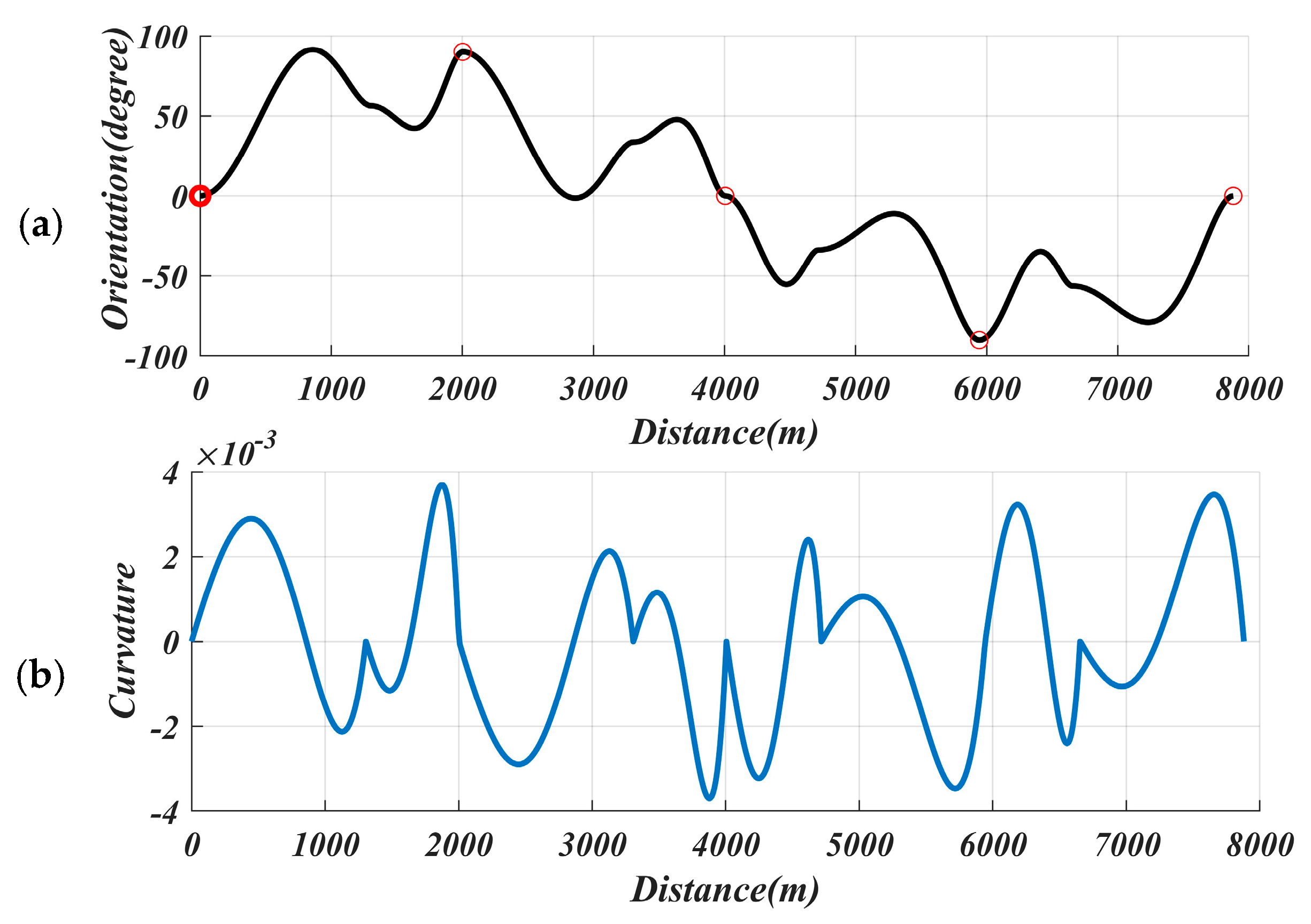
6.1. Results in Path Planning

In Figure 1a, the AMSV must go through the following points in order: start $[0,0,0°,0]$, point 1 $[1000,1500,90°,0]$, point 2 $[2500,2500,0°,0]$, point 3 $[4000,1500,-90°,0]$, and the end $[5000,0,0°,0]$, all marked with the red circle. Applying the methodology of the spiral path generator described in Algorithm 1 to generate the planned path shown in the green line, and the blue arrow shows the waypoint direction for each point. The AMSV can start from the start point and reach all the target navigation points successfully.

The method proposed here places a strong emphasis on optimizing path curvature during both global and local planning, focusing on the continuity of curvature and orientation angles. This approach effectively mitigates issues such as excessive tracking errors and reduced stability that can arise from discontinuities in angles. As illustrated in Figure 4, the results of the orientation and curvature planning demonstrate how the path planning for multiple target points achieves continuity in the path. Each target point’s angle and curvature are distinctly presented, showcasing the effectiveness of this method in ensuring a smooth trajectory. In conclusion, this method can generate a path with a continuous tangential angle that meets the design index constraints.

6.2. Results in Path Following

The AMSV system estimates the disturbance caused by ocean waves and is denoted as $\widehat{d}$, then compares it with the actual disturbance, denoted by $d$. The difference between them, denoted by $\tilde{d}$. Details are demonstrated in Figure 5, $\tilde{d}$ is kept within a reasonable range, further illustrating that the proposed AMSV system’s estimation value matches the actual disturbance.

Figure 6 gives the estimation of sideslip angle and surge velocity. It shows that the initial time has a large error, almost $2^{°}$. As time goes on, the estimate becomes more precise, and it reaches the exact sideslip angle at $0.2 \mathrm{s}$. The designed ESO can achieve the estimation of the changing unknown sideslip angle and compensate it in the GDL. This makes the path following more accurate. Additionally, the system can also follow the real angular velocity in a fast and stable way, and keep the error value within a reasonable range.

For AMSV, the external disturbance caused by the waves is the environmental factor interference it has to face. It can be seen from Figure 5 and Figure 6 that the algorithm proposed in this paper can estimate the disturbances in the sideslip angle, yaw, and sway directions of the AMSV, and then eliminate them in the controller design stage. Since the error of the disturbance estimation will gradually converge, the controller can eventually reduce the tracking error to the set range within a limited time and achieve accurate path following.

6.3. Comparison Among Different Methods

The performance of the proposed method, adaptive LOS (ALOS), and integral LOS (ILOS) in path-following control are compared and shown in Figure 7. The path-following controller proposed here performs well under the condition of random wave interference and model uncertainty and obtains good control performance.

For performance comparison, the following path-following controllers are used [33]:

• Parameters of the proposed controller in this article are given at the beginning of Section 6.
• For ALOS, it is assumed that the sideslip angle is measurable, so there is no side slip angle estimation module. This paper uses the method shown in reference [34] to compare with the proposed controller.
• For ILOS, an integral term is introduced to reduce the impact of the side slip angle, so there is no side slip angle estimation module. At the same time, it is an error-based adjustment method and cannot further improve the system tracking accuracy, which is very important for obstacle avoidance. This paper introduces the method shown in paper [7] and compares it with the proposed controller.

Figure 8 shows the details of the $x_e$ and $y_e$. These three GDLs can make the nonlinear AMSV track the target with a large initial error ($y\approx 30 \mathrm{m}$) and reduce the errors in $x_e$ and $y_e$. However, the ILOS-GDL method has excessive overshoots, which affects the control quality. The ALOS-GDL method has large oscillations during convergence. The proposed method outperforms both in terms of settling time and overshoot, as shown in

Table 1. Comparison results in the transient state.

	Settling Time (s)	Overshot
ALOS	381	15.8%
ILOS	304	29.2%
Proposed method	45.17	1.12%

.

Table 2. Comparison results in a steady state.

		Maximum Error	RMS
${\mathit{y}}_{\mathit{e}}\left(\mathit{m}\right)$	ALOS	4.7684	0.6520
	ILOS	8.7522	1.2627
	Proposed method	0.3391	0.0151
${\mathit{x}}_{\mathit{e}}\left(\mathit{m}\right)$	ALOS	0.2587	0.0266
	ILOS	0.4267	0.0440
	Proposed method	0.1176	0.0047

indicates that the proposed method can improve the stability and accuracy of the AMSV in path following.

Compared with ALOS and ILOS, the control algorithm proposed in this paper has significant improvements in stabilization time and overshoot. The stabilization time is reduced by 6 times and 26 times compared with ALOS and the overshoot is reduced by 14 times and 26 times compared with ILOS. In terms of maximum error, both ALOS and ILOS exceed 4 m, while the method proposed in this paper controls the error within 0.5 m, which is improved by 8 times, greatly improving the safety performance in the autonomous driving process.

6.4. Robustness to Uncertainty

Choosing the MAV mass parameter to test how the control is affected by mass variation is shown in Figure 9. The vessel mass is changed into ${\displaystyle \raisebox{1ex}{$5$}\!\left/ \!\raisebox{-1ex}{$6$}\right.} \mathrm{m}$, and ${\displaystyle \raisebox{1ex}{$7$}\!\left/ \!\raisebox{-1ex}{$6$}\right.} \mathrm{m}$, separately from the original value.

From the analysis in

Table 3. The maximum and average values of the $cte$ resulting from changes in quality.

	Mass	The Absolute Value of the Maximum Error	RMS
$cte \left(\mathrm{m}\right)$	${\displaystyle \raisebox{1ex}{$5$}\!\left/ \!\raisebox{-1ex}{$6$}\right.} \mathrm{m}$	0.4326	0.0876
	$m$	0.3391	0.0151
	${\displaystyle \raisebox{1ex}{$7$}\!\left/ \!\raisebox{-1ex}{$6$}\right.} \mathrm{m}$	0.6912	0.0978

, we can see that the uncertainty introduced by the mass change leads to a decrease in tracking accuracy. However, when the mass decreases by 1/6, the maximum error increases by 0.0935 m, and the average error increases by 0.0725 m; when the mass increases, the maximum error increases by 0.3521 m, and the average error increases by 0.0827 m. This shows that the disturbance caused by the mass decrease has a much greater impact on the controller than the disturbance caused by the mass increase. The maximum error is more than 3 times (from 0.0935 to 0.3521), while the average error is not much different (from 0.0725 to 0.0827). This shows that even if the mass change exceeds 15%, the tracking error is still stably controlled within 0.1 m, and the average error does not change significantly during the tracking process, ensuring safety during the operation. This shows that the controller can withstand the disturbance caused by the uncertainty of the internal parameters of the AMSV hull, thus confirming its robustness to disturbances.

6.5. Obstacle Avoidance

In Figure 10, the black line is the reference path, the blue line is the obstacle (crossing the reference line), and the green line is the real-time obstacle avoidance path based on global path planning. The green line deviates from the reference path and maintains a safe distance from the obstacle. The brown and yellow lines represent ALOS and ILOS, respectively. During the tracking process, ILOS is far from the green line and very close to the obstacle, reducing driving safety. ALOS is farther from the reference line but also vibrates more than the method proposed in this paper. Since the green line is the optimal path, more vibration means more deviation and longer convergence time. This also wastes more energy and lowers the safety of autonomous driving. Furthermore, ALOS and ILOS may encounter turbulence when they follow a new planned path after meeting an obstacle in the $70s$, which affects their driving safety and control stability, as shown in $y_e$ and $x_e$.

Based on the electronic navigational chart (ENC) data, several common navigation scenarios of the ocean environment map have been built in MATLAB 2022, such as coast, island, and reef. In these maps, the white is the navigable area of the ship, the black is the non-navigable area.

Results are given in Figure 11, where the green line is the planned path, the arrow shows the direction of the AMSV, and the red line segment is the actual track. As can be seen from Figure 10, in the actual driving process, The AMSV controlled by our method can accurately track the planned path, control the hull to turn in advance when encountering obstacles, return to the initial planned path immediately after avoiding obstacles, and then approach the original planned path on the premise of safe driving, which conforms to the continuous navigation between multiple points proposed in this paper.

7. Conclusions

This paper studies the multi-target path following task for the AMSV, which faces the challenges of unknown sideslip angle and system uncertainties. The models of the path-following task is proposed, and then a closed-loop structure is developed with three components: a multi-objective path planning algorithm with obstacle avoidance, a finite-time LOS-GDL, and a robust finite-time dynamics controller. The path planning algorithm produces a smooth, continuous path that sequentially passes through all the waypoints. The paper also presents an obstacle avoidance planning algorithm that ensures safety during driving. A finite-time ESO estimates the unknown sideslip angle online and feeds it to the nonlinear feedback LOS guidance, which converges in finite time. A finite-time surge and heading controller is used to make the nonlinear AMSV track the target quickly and accurately. The simulation results demonstrate that the path planning algorithm generates a satisfactory path that meets all the requirements and has less overshoot. The LOS-GDL converges faster, and the controller allows the autopilot system to track the velocity and course angle well. The obstacle avoidance path planning method can create a smooth and energy-efficient obstacle avoidance path based on the reference trajectory in less than 0.1 s, meeting the real-time requirements. The control algorithm proposed in this paper reduces the stabilization time by 6 times compared with ALOS and ILOS and reduces the overshoot by 14 times compared with ALOS and 26 times compared with ILOS. In terms of the maximum error, both ALOS and ILOS exceed 4 m, while the one proposed in this paper is stable within 0.5 m, which is 8 times different, greatly improving the safety performance during autonomous driving. This work comprehensively investigates the multi-target path following task for AMSV. The proposed methods and algorithms show their effectiveness through simulation results, providing improved path planning, guidance, and control capabilities for enhanced marine surface vessel navigation performance.

The main plans for future work are as follows:

(1). Using network learning methods such as deep reinforcement learning, we provide basic data sets and safety assurance.

(2). Deploy autonomous driving systems on multiple MSVs to achieve collaborative driving, thereby saving energy and improving traffic efficiency.

(3). Optimize the solution method to ensure that the calculation time is not limited by the number of target points, to achieve real-time operation.

References

1. Sun, X.; Wang, G.; Fan, Y. Model Identification and Trajectory Tracking Control for Vector Propulsion Unmanned Surface Vehicles. Electronics 2020, 9, 22. [Google Scholar] [CrossRef]
2. Dubins, L.E. On Curves of Minimal Length with a Constraint on Average Curvature, and with Prescribed Initial and Terminal Positions and Tangents. Am. J. Math. 1957, 79, 497–516. [Google Scholar] [CrossRef]
3. Lekkas, A.M.; Fossen, T.I. Integral LOS Path Following for Curved Paths Based on a Monotone Cubic Hermite Spline Parametrization. IEEE Trans. Control Syst. Technol. 2014, 22, 2287–2301. [Google Scholar] [CrossRef]
4. Peng, Z.; Wang, C.; Yin, Y.; Wang, J. Safety-Certified Constrained Control of Maritime Autonomous Surface Ships for Automatic Berthing. IEEE Trans. Veh. Technol. 2023, 72, 8541–8552. [Google Scholar] [CrossRef]
5. Healey, A.J.; Lienard, D. Multivariable sliding mode control for autonomous diving and steering of unmanned underwater vehicles. IEEE J. Ocean. Eng. 1993, 18, 327–339. [Google Scholar] [CrossRef]
6. Gu, N.; Wang, D.; Peng, Z.; Wang, J.; Han, Q.L. Advances in Line-of-Sight Guidance for Path Following of Autonomous Marine Vehicles: An Overview. IEEE Trans. Syst. Man Cybern. Syst. 2023, 53, 12–28. [Google Scholar] [CrossRef]
7. Caharija, W.; Pettersen, K.Y.; Bibuli, M.; Calado, P.; Zereik, E.; Braga, J.; Gravdahl, J.T.; Sorensen, A.J.; Milovanovic, M.; Bruzzone, G. Integral Line-of-Sight Guidance and Control of Underactuated Marine Vehicles: Theory, Simulations, and Experiments. IEEE Trans. Control Syst. Technol. 2016, 24, 1623–1642. [Google Scholar] [CrossRef]
8. Han, J. From PID to Active Disturbance Rejection Control. IEEE Trans. Ind. Electron. 2009, 56, 900–906. [Google Scholar] [CrossRef]
9. Han, Y.; Li, J.; Wang, B. Event-Triggered Active Disturbance Rejection Control for Hybrid Energy Storage System in Electric Vehicle. IEEE Trans. Transp. Electrif. 2023, 9, 75–86. [Google Scholar] [CrossRef]
10. Gao, S.; He, B.; Zhang, X.; Wan, J.; Mu, X.; Yun, T. Cruise Speed Estimation Strategy Based on Multiple Fuzzy Logic and Extended State Observer for Low-Cost AUV. IEEE Trans. Instrum. Meas. 2021, 70, 1–13. [Google Scholar] [CrossRef]
11. Liu, L.; Wang, D.; Peng, Z. ESO-Based Line-of-Sight Guidance Law for Path Following of Underactuated Marine Surface Vehicles With Exact Sideslip Compensation. IEEE J. Ocean. Eng. 2017, 42, 477–487. [Google Scholar] [CrossRef]
12. Li, J.; Sun, J.; Chen, G. A Multi-Switching Tracking Control Scheme for Autonomous Mobile Robot in Unknown Obstacle Environments. Electronics 2020, 9, 42. [Google Scholar] [CrossRef]
13. Kim, J.; Lee, C.; Chung, D.; Kim, J. Navigable Area Detection and Perception-Guided Model Predictive Control for Autonomous Navigation in Narrow Waterways. IEEE Robot. Autom. Lett. 2023, 8, 5456–5463. [Google Scholar] [CrossRef]
14. Guan, W.; Wang, K. Autonomous Collision Avoidance of Unmanned Surface Vehicles Based on Improved A-Star and Dynamic Window Approach Algorithms. IEEE Intell. Transp. Syst. Mag. 2023, 15, 36–50. [Google Scholar] [CrossRef]
15. Yao, P.; Zhao, R.; Zhu, Q. A Hierarchical Architecture Using Biased Min-Consensus for USV Path Planning. IEEE Trans. Veh. Technol. 2020, 69, 9518–9527. [Google Scholar] [CrossRef]
16. Wang, N.; Xu, H. Dynamics-Constrained Global-Local Hybrid Path Planning of an Autonomous Surface Vehicle. IEEE Trans. Veh. Technol. 2020, 69, 6928–6942. [Google Scholar] [CrossRef]
17. Meng, J.; Humne, A.; Bucknall, R.; Englot, B.; Liu, Y. A Fully-Autonomous Framework of Unmanned Surface Vehicles in Maritime Environments Using Gaussian Process Motion Planning. IEEE J. Ocean. Eng. 2023, 48, 59–79. [Google Scholar] [CrossRef]
18. Wang, N.; Zhang, Y.; Ahn, C.K.; Xu, Q. Autonomous Pilot of Unmanned Surface Vehicles: Bridging Path Planning and Tracking. IEEE Trans. Veh. Technol. 2022, 71, 2358–2374. [Google Scholar] [CrossRef]
19. Yu, Y.; Guo, C.; Yu, H. Finite-Time PLOS-Based Integral Sliding-Mode Adaptive Neural Path Following for Unmanned Surface Vessels With Unknown Dynamics and Disturbances. IEEE Trans. Autom. Sci. Eng. 2019, 16, 1500–1511. [Google Scholar] [CrossRef]
20. Rout, R.; Chi, R.; Yan, W. Sideslip-Compensated Guidance-Based Adaptive Neural Control of Marine Surface Vessels. IEEE Trans. Cybern. 2022, 52, 2860–2871. [Google Scholar] [CrossRef]
21. Piao, Z.; Guo, C.; Sun, S. Adaptive Backstepping Sliding Mode Dynamic Positioning System for Pod Driven Unmanned Surface Vessel Based on Cerebellar Model Articulation Controller. IEEE Access 2020, 8, 48314–48324. [Google Scholar] [CrossRef]
22. Sun, Z.; Zhang, G.; Yi, B.; Zhang, W. Practical proportional integral sliding mode control for underactuated surface ships in the fields of marine practice. Ocean Eng. 2017, 142, 217–223. [Google Scholar] [CrossRef]
23. Hao, L.; Zhang, H.; Yue, W.; Li, H. Fault-tolerant compensation control based on sliding mode technique of unmanned marine vehicles subject to unknown persistent ocean disturbances. Int. J. Control Autom. Syst. 2020, 18, 739–752. [Google Scholar] [CrossRef]
24. Tabataba’i-Nasab, F.S.; Moosavian, S.A.A.; Khalaji, A.K. Tracking Control of an Autonomous Underwater Vehicle: Higher-Order Sliding Mode Control Approach. In Proceedings of the 2019 7th International Conference on Robotics and Mechatronics (ICRoM), Tehran, Iran, 20–21 November 2019. [Google Scholar]
25. Guerrero, J.; Chemori, A.; Torres, J.; Creuze, V. Time-delay high-order sliding mode control for trajectory tracking of autonomous underwater vehicles under disturbances. Ocean Eng. 2023, 268, 113375. [Google Scholar] [CrossRef]
26. Zwierzewicz, Z. Robust and Adaptive Path-Following Control of an Underactuated Ship. IEEE Access 2020, 8, 120198–120207. [Google Scholar] [CrossRef]
27. Zhu, Y.; Li, Y.; Zeng, K.; Huang, L.; Huang, G.; Hua, W.; Wang, Y.; Gao, X. Finite-Time Cooperative Control for Vehicle Platoon With Sliding-Mode Controller and Disturbance Observer. IEEE Trans. Intell. Transp. Syst. 2022, 71, 7186–7201. [Google Scholar] [CrossRef]
28. Bhat, S.P.; Bernstein, D.S. Finite-time stability of continuous autonomous systems. SIAM J. Control Optim. 2020, 38, 751–766. [Google Scholar] [CrossRef]
29. Yang, C.W.J.; Guo, L.; Li, S. Disturbance-observer-based control and related methods-an overview. IEEE Trans. Ind. Electron. 2016, 63, 1083–1095. [Google Scholar]
30. Wang, L.; Xu, C.; Cheng, J. Robust Output Path-Following Control of Marine Surface Vessels with Finite-Time LOS Guidance. J. Mar. Sci. Eng. 2020, 8, 275. [Google Scholar] [CrossRef]
31. Stellato, B.; Banjac, G.; Goulart, P.; Bemporad, A.; Boyd, S. OSQP: An operator splitting solver for quadratic programs. Math. Program. Comput. 2020, 12, 637–672. [Google Scholar] [CrossRef]
32. Fossen, T.I. Guidance and Control of Ocean Vehicles; Wiley: New York, NY, USA, 1994. [Google Scholar]
33. Viadero-Monasterio, F.; Nguyen, A.T.; Lauber, J.; Boada, M.J.L.; Boada, B.L. Event-Triggered Robust Path Tracking Control Considering Roll Stability Under Network-Induced Delays for Autonomous Vehicles. IEEE Trans. Intell. Transp. Syst. 2023, 24, 14743–14756. [Google Scholar] [CrossRef]
34. Liu, F.; Shen, Y.; He, B.; Wang, D.; Wan, J.; Sha, Q.; Qin, P. Drift angle compensation-based adaptive line-of-sight path following for autonomous underwater vehicle. Appl. Ocean Res. 2016, 93, 799–808. [Google Scholar] [CrossRef]
Figure 1. The framework of the whole ASMV system, (a) global path planner (b) local path planner (c) LOS guidance geometry (d) finite-time LOS guidance (e) robust controller.
Electronics 14 00896 g001
Figure 2. Structure of the proposed methodology.
Electronics 14 00896 g002
Figure 3. The demonstration of the wave interference.
Electronics 14 00896 g003
Figure 4. The change curve of the reference path (a) Tangent path angle (b) curvature.
Electronics 14 00896 g004
Figure 5. The external disturbance.
Electronics 14 00896 g005
Figure 6. The vessel motion estimation.
Electronics 14 00896 g006
Figure 7. Comparison results of the path-following control.
Electronics 14 00896 g007
Figure 8. Control performance.
Electronics 14 00896 g008
Figure 9. The control performance with vessel mass variation.
Electronics 14 00896 g009
Figure 10. Control results of the obstacle avoidance.
Electronics 14 00896 g010
Figure 11. Testing ocean maps of common navigation scenarios: (a) coast (b) island (c) reef.
Electronics 14 00896 g011