Hierarchical Traffic Engineering in 3D Networks Using QoS-Aware Graph-Based Deep Reinforcement Learning

Abstract

Ubiquitous connectivity is envisioned through the integration of terrestrial (TNs) and non-terrestrial networks (NTNs). However, NTNs face multiple routing and Quality of Service (QoS) provisioning challenges due to the mobility of network nodes. Distributed Software-Defined Networking (SDN) combined with Multi-Agent Deep Reinforcement Learning (MADRL) is widely used to introduce programmability and intelligent Traffic Engineering (TE) in TNs, yet applying DRL to NTNs is hindered by frequently changing state sizes, model scalability, and coordination issues. This paper introduces 3DQR, a novel TE framework that combines hierarchical multi-controller SDN, hierarchical MADRL based on Graph Neural Networks (GNNs), and network topology predictions for QoS path provisioning, effective load distribution, and flow rejection minimisation in future 3D networks. To enhance SDN scalability, introduced are metrics and path operations abstractions to facilitate domain agents coordination by the global agent. To the best of the authors’ knowledge, 3DQR is the first routing scheme to integrate MADRL and GNNs for optimising centralised routing and path allocation in SDN-based 3D mobile networks. The evaluations show up to a 14% reduction in flow rejection rate, a 50% improvement in traffic distribution, and effective QoS class prioritisation compared to baseline techniques. 3DQR also exhibits strong transfer capabilities, giving consistent performance gains in previously unseen environments.

1. Introduction

One of the key targets of the 6th Generation (6G) mobile network is ubiquitous coverage and broadband network access worldwide [1]. While extending the terrestrial infrastructure in remote locations is often infeasible due to financial, physical, or legal reasons, network omnipresence is expected to be achieved via the integration of Terrestrial Networks (TNs) and Non-Terrestrial Networks (NTNs) [2,3,4], including both aerial and satellite systems. Nowadays, carrier-grade aerial networks are largely limited and correspond mainly to High Altitude Platform Systems (HAPSs) or ad hoc networks based on Unmanned Aerial Vehicles (UAVs) (set up dynamically during natural disasters, mass events, etc.). Currently, the primary interest lies in the integration of TNs with already operating satellite systems with a focus on Low Earth Orbit (LEO) systems due to acceptable latency (30–50 ms) [5].

The LEO networks, however, introduce several challenges caused by the fast mobility of infrastructure causing frequent topology changes [6] and severe capacity constraints—both Inter-Satellite Links (ISLs) and Feeder Links (FLs). To maintain service continuity and economise NTN resources, it is necessary to adopt intelligent Traffic Engineering (TE) for Quality of Service (QoS) routing, End-to-End (E2E) cross-layer operations, and network-wide load balancing. The latter is critical to mitigating the impact of the disappearing links and related distribution of rerouted traffic across multiple links (not necessarily the closest ones as in shortest path routing). In TNs, Deep Reinforcement Learning (DRL) is a common candidate method for TE due to high performance and adaptability [7,8]. Its application in NTNs is, however, problematic due to the strong dependence of the learned policies on the problem setup. Time-variant environments complicate the exploitation of traditional “deep” architectures and degrade DRL’s models convergence. Moreover, DRL faces observability and scalability issues, and its usage in distributed and decentralised environments is still being heavily researched [9,10,11,12].

Software Defined Networking (SDN) is often perceived as a vital concept to introduce flexibility into the network and facilitate cross-layer integration [13]. The logically centralised software-driven control, support for TE, and capabilities to leverage contextual information are essential to optimise networking in the evolving NTN segment. The usage of SDN in carrier-grade networks is, however, still limited due to scalability, interoperability [14], and SDN Controller (SDNC) placement issues [15]. While distributed architectures address the above partially, they complicate E2E TE and E2E QoS management and require SDNCs coordination.

In this paper, based on the authors’ previous work [16], proposed is a novel TE approach called 3D QoS-Aware Routing (3DQR) for optimising routing and path allocation in future mobile Three Dimension (3D) networks. The key contributions of this paper are as follows:

• Considering the heterogenous and distributed character of emerging 6th Generation (6G) networks, introduced is a TE framework based on distributed (multi-controller) hierarchical SDN and Multi-Agent Deep Reinforcement Learning (MADRL), which enables flexible global and per-segment optimisation of 3D networks (i.e., comprising terrestrial, aerial, and satellite segments). The proposed framework improves load distribution and flow acceptance rate while considering QoS requirements of individual flows and traffic priorities. Moreover, 3DQR tries to minimise the number of broken paths and path reconfigurations to reduce session disruptions and SDN Control Plane (CP) overhead to improve SDN scalability
• A hierarchical MADRL routing and path allocation strategy is developed, which involves intelligent DRL-Graph Neural Network (GNN) TE agents leveraging message passing and attention mechanisms as well as network topology predictions to improve the reasoning of agents and adaptability to frequently changing 3D network topology.
• Based on evaluation, an over 13% reduction in flow rejection rate and a 50% improved load distribution compared to baseline routing methods are demonstrated. Also, strong generalisation and transfer capabilities of 3DQR agents are demonstrated, which enable their effective exploitation in previously unseen topologies.

The paper is structured as follows. Section 2 outlines key routing challenges in 3D networks. Section 3 describes related works on TE focusing on SDN-based frameworks, QoS enforcement, and DRL applications. Section 4 presents the 3DQR architecture, principles, and E2E path establishment workflow. Section 5 presents the details of the 3DQR algorithm, including mathematical formulation, DRL problem setup, agent architecture, and E2E operation. Section 6 describes the evaluation and obtained results. Section 7 outlines open issues and potential future works. Finally, Section 8 summarises and concludes the paper.

2. Routing Challenges in TN-NTN Mobile Networks

Integration of terrestrial, aerial, and satellite network segments will enable an omnipresent network. Fast mobility of the satellite part poses several challenges and issues regarding the organisation of routing and its optimisation. The key challenges to be tackled to enable unified 3D networks include the following [3,5,17]:

(C1)

Routing convergence—applying traditional Internet Protocol (IP) routing schemes, e.g., Open Shortest Path First (OSPF), is problematic in NTNs due to mobility of network nodes. Frequent reconfigurations of connections between nodes require continuous updates of routing tables and link costs to maintain up-to-date information on the network state within the nodes. The changes occur repeatedly, causing almost constant updates, which impacts the convergence and leads to unstable routing and large signalling overhead [18]. Adoption of SDN to provide dynamic and flexible user traffic steering is a common solution [18]. However, the original SDN concept lacks CP scalability, so its wide-scale deployments are problematic. Distributed SDN architectures allow for mitigating SDNC overload at the cost of complexity—E2E functionality requires the development of coordination mechanisms across multiple SDNCs. Also, in wide-scale deployments, SDNCs placement for optimal network control needs careful consideration (in terms of both intra- and cross-layer CP latency, network observability (obtaining reliable network monitoring information), and recovery).

(C2)

Temporal and predictive routing—topology changes caused by the mobile NTN nodes can lead to broken links or changes of link properties (e.g., bandwidth drops due to partial occlusion). Addressing these issues will require frequent rerouting of flows and path updates on a topology change, leading to extensive signalling traffic. To calculate viable routes with increased durability and mitigate the above issues, link availability prediction and mechanisms for fast updates of paths (via low-latency monitoring, TE metrics adjustments, etc.) are vital. These are required to support time-scheduled routing schemes and enhancements by contextual information (e.g., satellite orbits, air interfaces alignment, object occlusion, etc.).

(C3)

Resilience—the disappearing links and broken network paths can lead to severe Service Level Agreement (SLA) violations. Hence, increasing resilience to minimise the impact of communication cutoffs is a core requirement to enable QoS-driven services. Potential solutions include multi-path and/or node/edge-disjoint routing [19], in-switch buffering mechanisms in case of access node isolation (i.e., store-and-forward) [20,21], or predictive routing schemes.

(C4)

Optimisation—conventional TE algorithms—e.g., Multi-Protocol Label Switching—Traffic Engineering (MPLS-TE)—cannot be used effectively in NTNs due to long convergence time. The emerging routing and TE methods will need to consider both QoS constraints and effective traffic distribution to handle limited ISL capacity. Moreover, the synchronisation of network state information across TE databases and its unified representation in NTNs becomes crucial to facilitate E2E control and Artificial Intelligence (AI)-driven optimisation. To achieve the latter, the TE algorithms need to be able to extract the information from the nodes and link relationships rather than the fixed graph structure to avoid overly complex and monolithic models.

(C5)

Asset heterogeneity—future mobile networks are expected to combine heterogeneous systems with diversified service capabilities and properties (radio interfaces, protocol stack, etc.), i.e., the Network of Networks [22]. To enable E2E services in 3D networks, it is essential to develop dynamic QoS management and coordination mechanisms to provide paths satisfying E2E QoS regimes. Also, to handle the rising complexity, the network management will need to embed automated and intelligent TE mechanisms enabling cross-domain cooperation, knowledge transfer to new segments, and seamless operation.

3. Related Work

In recent years, many works addressing the problems of intelligent TE in TNs, NTNs, and integrated 3D networks have been published. Here, in focus are key routing algorithms and architectural frameworks that target optimisation under QoS constraints.

Organisation of routing is one of the key issues regarding carrier-grade NTNs. In traditional TNs, routers calculate routing tables using a routing information database established based on network topology and link states. Routing updates require exchanging topology information across network devices. It leads to significant overhead and slow convergence [23], causing the inapplicability of traditional approaches in NTN scenarios due to limited resources and frequent topology changes. Therefore, academia and industry started to develop routing algorithms adapted to the NTN specificity [24]. A time–topology routing algorithm for 3D networks is presented in [25], which outperforms existing message-based routing methods in terms of latency and delivery rate. The method considers node mobility and contextual information (weather, propagation models, etc.) to obtain a time-based inter-node visibility and link information to construct the network topology for a certain time frame and generate routes providing stable communication. A QoS-aware routing minimising congestion in SDN-based NTN systems is proposed in [26]; the method assigns scores to network links based on selected QoS parameters (e.g., utilisation, congestion degree, delay). On that basis, it finds shortest paths using a modified Bresenham’s algorithm. A compass time–space model for the scalable representation of mass-scale NTN systems and the QoS routing method is introduced in [27]. The algorithm yields QoS performance and reliability improvements compared to baseline methods. A cooperative data downloading routing scheme for LEO satellites, which uses ISL to schedule feeder link bandwidth resources, is proposed in [28]. The routing algorithm considers the limited ISL bandwidth and utilises linear programming for solving the route selection problem. Another popular NTN routing approach to provide resilience and stable QoS involves exploiting multi-path routing. A Multi-Path routing algorithm with Joint Optimisation of Load balancing (MPJOL) [29] proposes clustering of LEO satellites and selection of cluster head nodes (considering connectivity and load capacity) to reduce the network scale, and calculating k-shortest paths between the source and destination clusters. The method improves transmission efficiency and quality while reducing the route discovery overheads. The Multi-Path QoS Routing (MPIR) approach given in [30], which targets QoS improvements, proposes an algorithm to generate QoS routes using a genetic algorithm fueled by simulated annealing to handle population diversity and improve convergence. While increasing resilience, multi-path routing is, however, inefficient in large-scale networks [29] due to traffic multiplication. Another common dynamic routing approach is to embed the information about the routes within the packets and exploit Source Routing (SR) [31] or Segment Routing [32]. These solutions, however, increase the Data Plane (DP) traffic volume due to additional headers attached to each conveyed packet. Also, SR-based methods require continuous updates of preset paths in gateway nodes, which can result in significant operational overhead.

With the recent onset of AI and Machine Learning (ML), more researchers have directed their attention towards using AI-based routing in complex environments such as Space-Air-Ground Integrated Networks (SAGINs) [33]. AI-driven routing (commonly DRL-based) typically aims to solve specific issues of conventional routing methods in dynamic topologies, i.e., convergence, QoS, and resource efficiency. A two-hops state-aware Double Deep Q-Network (DDQN)-based routing strategy for LEO networks called DRL-THSA [34] assumes that a node needs only link-state information of neighbouring nodes up to two hops away for the prediction of the next hop. The approach shows solid performance regarding the E2E delay, throughput, packet drop rate, and traffic distribution. A DRL-based satellite routing method solving multiple path requests at once to minimise latency is proposed in [35]. The centralised DRL, however, does not offer high performance, especially in wide-scale network deployments in which components are spatially distant due to network observability issues. Therefore, to optimise complex and distributed networks, such as NTN and 3D networks, a common approach is to use Multi-Agent Deep Reinforcement Learning (MADRL) methods featuring flat or hierarchical structures. A two-stage MADRL framework has been introduced for mobile edge computing [11], which employs high-level agents for the optimisation of transmitting power and duration of wireless transfer power, and low-level agents to improve offloading decisions of wireless devices, time allocation for offloading, and used computing resources. A distributed routing algorithm based on the Transformer-MIX architecture and MADRL, which optimises E2E latency and load balancing, has been proposed [9]. In the concept, the LEO satellites can make individual next-hop decisions for the packets in real-time while participating in the centralised training scheme focusing on load balancing. A MADRL approach, which uses agents enhanced with self-attention mechanisms to first better understand the semantics of network state and then optimise routing in LEO networks, has been proposed [10]. The method enables lowering E2E latency and improves average throughput compared to other distributed routing methods.

Another emerging trend in AI-driven routing is using GNNs for more efficient network state representation and predictions to fuel AI reasoning and performance. A method using GNNs is proposed to handle routing strategies devoted to finding the shortest path and maximising the minimum allocated bandwidth for improved load distribution across network links in [36]. Another approach uses GNNs to predict packet delay distribution and loss and uses these predictions for routing optimisation and network planning [37]. A Graph-Aware Deep Learning model is proposed [38] to maintain precise network measurements along with current positions and destinations of forwarding tasks. The Contact Graph Routing algorithm is proposed with a mix of reinforcement and Bayesian learning for delay-tolerant networks in [39]. A topology-aware GNN framework for link prediction highlighting the trade-offs between the algorithm precision and speed, which can also be used for routing, is introduced in [40]. Another GNN-based routing method for terrestrial optical networks combining Message Passing Neural Network (MPNN) and DRL is proposed in [41]. The method yields good performance and generalises well on unseen topologies. A graph-based MADRL approach called GraphPR has been proposed [12] to optimise routing in satellite networks with partial observability. The method employs Graph Attention Networks to transform satellite states (e.g., location, queue, neighbour states), which are later processed by MADRL to make routing decisions. Due to the increasing popularity of GNNs, a benchmark system aimed at accelerating the development of quality GNNs has been developed and described [42].

Clearly, 3D networks will comprise multi-tier, multi-dimensional and heterogeneous network architectures with different capabilities and properties that will complexify QoS-driven communication [43,44]. The most popular State of the Art (SotA) approach is the adoption of distributed architectures with extensions implementing E2E functionality via cross-domain coordination. A hybrid hierarchical and multi-controller SDN architecture to tackle resource management and minimise SDNC signalling overhead in heterogeneous 3D networks is proposed [43]. The SDNCs, handling ground, aerial, and satellite layers, caters towards layer-specific QoS requirements and routing, while the E2E routes are combined from the intra-layer ones in the service composition layer. Service-Customised Network (SCN) for Immersive Media in SAGINs is studied in [44]. The concept proposes hierarchical SDN deployment for increased management capabilities and usage of edge servers for reduced end-to-end latency. It also introduces a DRL-enhanced multi-path Transport Control Protocol (TCP) routing strategy, which uses network state as an input and user Quality of Experience as feedback. Another hierarchical multi-tier SDN-based framework for integrated vehicular networks is proposed in [45], which introduces multi-level SDNCs (local, regional, national, and global domains) that communicate to enable coordination across segments and optimise network services.

Summing up, SotA approaches strongly lean towards exploiting SDN for 3D network architectures. With increasing complexity, heterogeneity, and dynamics comes the need for efficient and tailored routing solutions. AI/ML-based methods, especially GNN-based ones, outperform conventional routing algorithms and enable good generalisation in complex environments. The latter is achieved thanks to the GNN ability to preserve the graph structure of data (compared to Deep Neural Network (DNN) architectures) and perform embedding operations. The node/edge feature embedding enables encoding of spatial and relational dependencies of the input data into low-dimensional space, taking into account not only the feature values but also the connectivity between nodes. In the context of DRL methods, GNNs bring multiple benefits that include learning meaningful state representations, improving output policy quality, reasoning, and model generalisation. As GNNs can process different-sized graphs, compared to traditional fixed-size DRL, they enable operation in frequently changing environments, such as NTNs and LEO, eliminating the need for multiple agents or complex architectures supporting state representation processing into a fixed-size input (as it would be in the DNN case).

While deeply investigated in SotA, the usage of GNNs and DRL for routing, and their benefits regarding performance, QoS provisioning, or load balancing, as well as the SDN CP overhead, scalability aspects, and operator, profits are usually overlooked. Moreover, there is a general lack of methods for AI-driven 3D routing that consider the performance of individual network segments in addition to the E2E one. Although numerous distributed routing approaches are proposed (also GNN-based ones), these usually focus on selecting the next hop, giving limited abilities in terms of global-level network optimisation. This gap is filled by proposing an intelligent QoS-aware routing approach for SDN-based 3D networks that optimises load distribution, considers network operator priorities, and limits the impact on the SDN CP caused by frequent rerouting.

4. 3D QoS-Aware Routing (3DQR)

4.1. Concept Principles

Infrastructure mobility and the mitigation of its effects are a core challenge for TN and NTN integration. Introducing User Plane (UP) flexibility and mechanisms for optimal routing and QoS path allocation is vital for provisioning stable network services to the end customers worldwide (cf. Section 2). The hereby proposed 3DQR concept aims to address this challenge by combining the powers of SDN, DRL, GNNs, and topology prediction. In 3DQR, a network comprised of a multi-stratum (terrestrial, aerial, space) and multi-domain (multi-controller) hierarchical SDN architecture is considered, as shown in Figure 1.

The network assets within strata (terrestrial, aerial, and satellite) form SDN domains (one or more per stratum). Each domain is controlled by a dedicated SDNC (one per domain), i.e., Terrestrial SDNCs (T-SDNCs), Aerial SDNCs (A-SDNCs), and Satellite SDNCs (S-SDNCs). SDNCs implement domain-specific CP protocols (e.g., OpenFlow (OF) [46]), enabling full control of the traffic flows within a domain (i.e., of SDN switches) and monitoring suite for network state information acquisition. Each SDNC is accompanied by a dedicated Domain QoS-aware Router (DQR) with embedded DRL-GNN Agent (DGA) (further described below)—TE application is responsible for the calculation of optimal routes for all of the flows traversing the domain and load distribution. The E2E functionality is implemented by the logically centralised and physically distributed global-level Main SDNC (M-SDNC) acting as the umbrella controller for the underlying set of SDNCs and assisted by Master QR (M-QR)—DQR equivalent handling cross-domain routing and load balancing. M-SDNC operates using the overlay network view of the network that refers to the following:

• Monitoring—in spatially distributed networks, centralised SDNC suffers from CP link latency, which leads to obtaining obsolete monitoring data. The hierarchical approach partially addresses this issue, as SDNCs can be deployed in close proximity of switches. Moreover, growing network size increases the monitoring data volume dramatically. Therefore, instead of link-level metrics, SDNCs calculate the parameters of overlay links between domain ingress/egress nodes denoted as Border Nodess (BNs) (access nodes, gateways, satellites, etc.; cf. Figure 1). This reduces the monitoring traffic while conveying information about domains’ abilities to serve new flows (cf. Section 5.1).
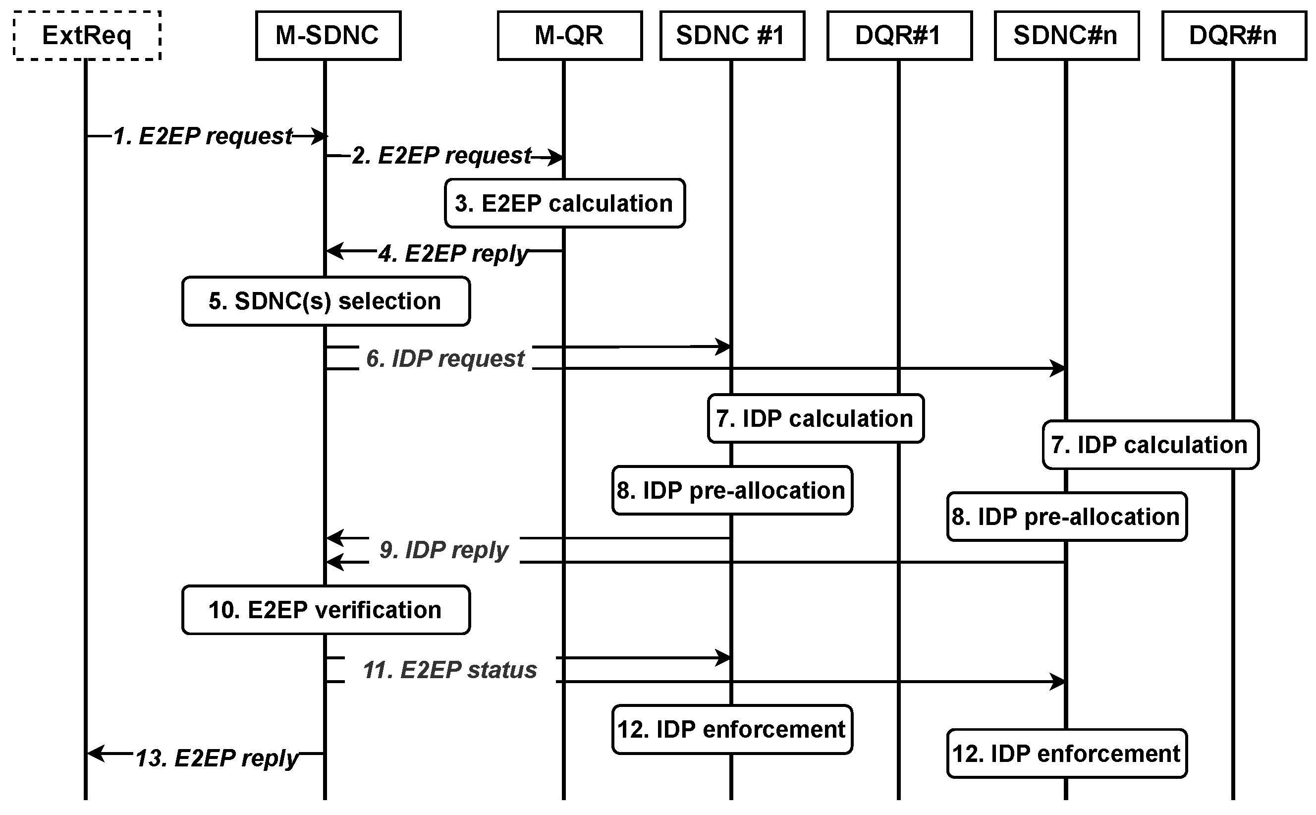
• CP operations—M-SDNC has a view limited to BNs, overlay links within domains, and interconnection links to domains. Hence, M-SDNC arranges the End-to-End Path (E2EP) enforcement by instructing individual SDNCs to allocate Intra-Domain Path (IDP) between BN pairs (i.e., a path composed of two BNs and intermediary relay nodes). As inter-domain links are either physical or overlay links between BNs of two domains, installing relevant flow entries in the BNs is equivalent to establishing the inter-domain path. The full E2EP allocation procedure is described in Section 4.2.

The topology information, monitoring metrics, and flow allocation history are stored in dedicated Traffic Engineering Databases (TEDs)—local and E2E—and exposed to TE applications on demand. TED implements the data retention strategies based on the requirements of operating TE mechanisms (especially DRL-GNN agents described further in this section). The details, however, are out of the scope of this paper.

The ultimate goal of 3DQR is to perform optimal routing and E2E path allocation in the integrated 3D network, considering three major aspects: network-level performance (measured by the degree of traffic distribution over the network links), flow QoS constraints, and flow importance (determined arbitrarily by the network operator based, e.g., on service priority or associated profits). These objectives are achieved by the federation of DQRs and a centralised M-QR, which provide optimal paths on SDNCs/M-SDNC requests (domain-level and E2E). Unlike traditional IP networking, where a router is a DP- and CP-integrating device that makes local packet routing decisions, in 3DQR, the router is an Application Plane (AP) function interacting with the SDNC’s NorthBound Interfaces (NBIs). The selection of the most profitable paths is made by the intelligent DGA implementing the DDQN algorithm [47] and embedded in each DQR/M-QR. The data flow within DQR and DGA is shown in Figure 2.

Upon the arrival of a path request (cf. Section 4.2), DQR collects the most recent network state information (e.g., OF-based statistics—cf. Section 5.2) and extends its node/edge feature vectors by additional node/link state information such as node centrality or nodes/links expiry information (probability of nodes’ reachability or existence of ISLs and gateway links in the considered time-frame). The latter is provided by a dedicated Geographic Information System-based Mobility Management Function (GIMMF) entity, which estimates NTN topology (active ISLs, FLs, etc.) and calculates the aggregated persistent graph within a time frame (i.e., containing only the set of nodes and links that is not expected to change), using the orbital/trajectory parameters of nodes. DQR computes then k shortest paths using delay as the metric. For each candidate path, DQR/M-QR performs virtual path allocation using flow’s QoS class requirements and feeds the outcome state to the DGA to obtain the value of the allocation. The path is selected based on the highest Q-value across k virtual path allocations. Additionally, to tackle the issue of variable size of network states in NTN, DGAs exploit the GNN architecture to extract the information about the relationship between nodes and links to enable effective routing regardless of topology shape and size (cf. Section 5.3).

It must be noted that SDNCs and M-SDNC are solely responsible for verifying the feasibility of a path and its enforcement while the reasoning is left to DQRs. Moreover, as each satellite/aerial node can act as an access point capable of serving the User Equipment (UE), they are considered BNs. Finally, to enable straightforward integration of the concept with 3rd Generation Partnership Project (3GPP) networks, QoS classes are aligned with the 3GPP definition, i.e., 5G QoS Identifier (5QI) [48].

4.2. E2E Routing and Path Allocation Approach

The paths are requested by the External Requester (ExtReq) entity (#1) such as UP entities, Management and Orchestration (MANO), M-SDNC applications, etc. M-SDNC, which constitute a single entry point to the framework by exposing path allocation Application Programming Interfaces (APIs). The E2EP allocation process is shown in Figure 3. The path allocation process also includes the reservation of resources for the traffic flow with respect to the flow’s QoS class.

First, M-SDNC sends the E2EP request containing flow-specific data (source node, target node, and QoS class) to M-QR (#2). M-QR calculates the E2EP (#3), which consists of BNs and overlay links visible at the M-SDNC level (#4). After verification of E2E path allocation feasibility, M-SDNC splits the path into segments based on the BNs domain membership (#5). For each segment, M-SDNC requests IDP calculation from the SDNC-DQR pairs (#6, #7). Then, IDPs’ feasibility is verified by SDNCs, which ends with the pre-allocation of resources of the flow (#8). Finally, SDNCs notify M-SDNC about the successful pre-allocation of resources for the IDPs (#9), including the QoS parameters of the selected paths (e.g., delay, expected error rate, etc.). After receiving a positive notification from each domain, M-SDNC verifies if connected IDPs satisfy the E2E QoS requirements (#10). If so, M-SDNC notifies respective SDNCs about successful E2EP verification (#11) to finalise enforcement (#12), and notifies ExtReq about successful allocation (#13). If IDP allocation is impossible, e.g., due to dynamic changes in the network (nodes mobility, faults, etc.), SDNC notifies M-SDNC about it; then, M-SDNC requests respective SDNCs to revert IDPs allocations. The same approach is taken by M-SDNC if E2EP verification fails.

While the centralised approach increases procedure duration, it ensures E2EPs even in disjoint NTN topology graphs, i.e., missing ISLs, or in a multi-stakeholder environment (e.g., NTN roaming). The inclusion of an M-SDNC overlay view enables routing the traffic via TN or other NTN segments to connect the disjoint parts of topology and attempt the allocation.

5. Algorithm

This section presents the details of the 3DQR algorithm and related mathematical formulations. 3DQR targets routing challenges in 3D networks (cf. Section 2) by carrying out the following:

• Using SDN-based deployment for flexible E2E routing and TE operations [C1, C4];
• Leveraging GIMMF-based predictions to improve DGA reasoning [C2] and to establish a topology containing stable links within a given time frame [C3];
• Providing a novel approach combining DDQN and GNN to (i) provide intelligent routing and path allocation decisions in 3D networks; (ii) enable variable size input; and (iii) embed both network- and flow-level metrics for evaluation of routing decisions [C4];
• Adopting a distributed SDN architecture and modular routers, enabling heterogeneous technologies at the domain level and dynamic attachment of new domains [C1, C5].

The 3DQR operation details are presented in the following sections.

5.1. System Model

The problem of QoS routing and path allocation in an integrated TN-NTN network is modelled as a time-expanded minimum-cost multi-commodity flow. The overall network graph $G(V,E,t)$ is composed of a set of domain sub-graphs, each belonging to a domain described by a unique identifier $\mathfrak{d}\in \mathbb{N}$. Each sub-graph is time-variant $G^{\mathfrak{d}}(V^{\mathfrak{d}},E^{\mathfrak{d}},t)$ in the NTN case (space and aerial strata) or time-invariant $G^{\mathfrak{d}}(V^{\mathfrak{d}},E^{\mathfrak{d}})$ in the TN case. The graphs are constituted by sets of nodes and edges, i.e., $V=[v_1,v_2,\dots v_j]$ and $E=[e_{12},e_{13},\dots e_{ij}]$, with $e_{ij}$ representing a bidirectional edge between vertices $v_i$ and $v_j$. Edge properties are described by a total of six features ($F=\left\{f_{ij}\right|(v_i,v_j)\in E\}\in {\mathbb{R}}^{\left|E\right|\times m}$, m—dimensionality of features) that include total capacity $c_{ij}$, total Guaranteed Flow Bit Rate (GFBR)—cf. [48], clause 5.7.2.5—allocated to flows $b_{ij}^{\mathrm{GFBR}}$, total Maximum Flow Bit Rate (MFBR)—cf. [48], clause 5.7.2.5—that can be consumed by flows $b_{ij}^{\mathrm{MFBR}}$, delay $d_{ij}$, packet error rate ${\delta }_{ij}$, link utilisation $u_{ij}=b_{ij}^{\mathrm{GFBR}}/c_{ij}$, indicating the fraction of capacity currently allocated to flows, and ${\zeta }_i$—the vector containing the share of flow types traversing the edge (one value per QoS class identifier). The nodes’ features ($X=\left\{x_i\right|v_i\in V\}\in {\mathbb{R}}^{\left|V\right|\times m}$) correspond to the ones defined for edges, i.e., including node capacity (cf. Equation (1)), guaranteeing the maximum bandwidth allocated to flows traversing the node (cf. Equations (2) and (3)) and node utilisation (cf. Equation (4)). The edges incident to the vertex $v_i$ are denoted with the $E\left(v_i\right)$ operator—i.e., $E\left(v_i\right)=\{e\in E:\exists v_j\in V,e=(v_i,v_j)\in E\}$. The delay and packet error rate are excluded from node features as they are both usually included in the link parameters due to measurement strategies that span over links and connecting switches egress/ingress ports [49]. The time consumed by switches on flow matching and forwarding is negligible and omitted.

$$\begin{array}{c}\hfill c_{v_i}=\sum _{e_{ij}\in E\left(v_i\right)}{c}_{ij}\end{array}$$

(1)

$$\begin{array}{c}\hfill b_{v_i}^{\mathrm{GFBR}}=\sum _{e_{ij}\in E\left(v_i\right)}{b}_{ij}^{\mathrm{GFBR}}\end{array}$$

(2)

$$\begin{array}{c}\hfill b_{v_i}^{\mathrm{MFBR}}=\sum _{e_{ij}\in E\left(v_i\right)}{b}_{ij}^{\mathrm{MFBR}}\end{array}$$

(3)

$$\begin{array}{c}\hfill u_{v_i}={\displaystyle \frac{b_{v_i}^{\mathrm{GFBR}}}{c_{v_i}}}\end{array}$$

(4)

The edge metrics are used by SDNCs to calculate the overlay view for M-SDNC/M-QR. The corresponding overlay metrics and topology are denoted with a superscript $\psi$. The metrics transformation takes into account only the BNs of the domain ($V^B\subset V$) so that M-SDNC sees the viable allocations between domain gateways. The bandwidth-related metrics between a pair of BNs, $v_i,v_j\in V^B$, are calculated using maximum flow (Ford–Fulkerson, Edmonds–Karp, Push–Relabel, etc.) and shortest path (e.g., Dijkstra) algorithms, denoted as $maxflow$ and $SP$, extending the concept [16]. These include the following:

• Total capacity $c_{ij}^{\psi }$ measured with no traffic between $v_i$ and $v_2$:

  $$\begin{array}{c}\hfill c_{ij}^{\psi }=maxflow(v_i,v_j)\end{array}$$

  (5)
• Aggregate of GFBRs allocated to flows $b_{ij}^{\psi ,GFBR}$:

  $$\begin{array}{c}\hfill b_{ij}^{\psi ,GFBR}=c_{ij}^{\psi }-maxflow(v_i,v_j)\end{array}$$

  (6)
• Peak aggregated bandwidth (aggregate of MFBRs) $b_{ij}^{\psi ,MFBR}$ that can be consumed by allocated flows:

  $$\begin{array}{c}\hfill b_{ij}^{\psi ,MFBR}=\left[lr\right]\sum _{(u,w)\in SP(v_i,v_j)}{b}_{uw}^{MFBR}\end{array}$$

  (7)
• Utilisation of overlay link $u_{ij}^{\psi }$ between $v_i$ and $v_j$:

  $$\begin{array}{c}\hfill u_{ij}^{\psi }=(c_{ij}^{\psi }-b_{ij}^{\psi ,GFBR)}/c_{ij}^{\psi }\end{array}$$

  (8)

The delay and packet error rate are approximated by calculating the shortest path obtained above and aggregation/multiplication over the edges belonging to the path:

$$\begin{array}{c}\hfill d_{ij}^{\psi }=\sum _{(u,w)\in SP(v_i,v_j)}{d}_{uw}\end{array}$$

(9)

$$\begin{array}{c}\hfill {\delta }_{ij}^{\psi }=1-\prod _{(u,w)\in SP(v_i,v_j)}(1-{\delta }_{uw})\end{array}$$

(10)

Each traffic flow is modelled by a tuple $f=(v_{src},v_{dst},t_0,t_d,q)$, where $v_{src}$—source, $v_{dst}$—sink, $t_0$—arrival time, $t_d$—duration, and $q_i$—an SDN-level QoS class. Following the simplified 3GPP 5QI definition, $q_i$ is modelled as a tuple $q_i=(b^{\mathrm{GFBR}},b^{\mathrm{MFBR}},d^{\max },{\delta }^{\max })$, where $q_{\mathrm{i}}$—a QoS class identifier (common across SDN domains/strata), $b^{\mathrm{GFBR}}$—GFBR (corresponding to the bandwidth reserved by SDNC/M-SDNC), $b^{\mathrm{MFBR}}$—MFBR, $d^{max}$—Packet Delay Budget (PDB) (cf. [48], clause 5.7.3.4), and ${\delta }^{max}$—Packet Error Rate (PER) (cf. [48], clause 5.7.3.5). Hereby, each flow is considered as unidirectional, due to commonly different proportions of uplink (UL) and downlink (DL) traffic. In such cases, allocation of two-way exchange requires using different $q_i$ values for UL and DL flows. Each allocation of flow f results in either acceptance or rejection decision $f_d\in 1,0$.

5.2. DRL Problem Setup

The multi-controller hierarchical SDN can be treated as the combination of standard Reinforcement Learning (RL) settings, i.e., a set of stochastic environments—each modelled as Markov Decision Process (MDP) represented by tuples $M=(S;A;T;R)$, where S denotes states, A actions that can be taken by the agent, T the transition function, and R the reward function. As the environment details are unknown, including transition probability between states and dynamics, the dynamic programming methods [50] cannot effectively solve the given MDP. Moreover, the network environment is a non-linear system (due to complex traffic patterns, bursty behaviour, in-DP buffering, etc.), making the exploitation of well-established methods inapplicable [51]. Hence, the proposed DQR algorithm utilises a model-free DRL due to its suitability for operation in environments in unknown or not-well-understood dynamics.

State: For each arriving flow allocation request, the DRL agent is to evaluate k candidate paths and select the one that maximises the reward. To improve the reasoning of agents, the environment state is obtained as follows. Once the network information is pulled from SDN controllers (i.e., edge/node properties listed in Section 5.1), the graph is extended with more features provided by GIMMF and calculated internally by the router (i.e., state enrichment phase). Additional features include the edge/node expiry ${\xi }_{ij},{\xi }_i\in \langle 0,1\rangle$ (probability of node/edge activity in the defined time horizon: 0 for active, 1 for inactive), $\chi \left(v\right)\in \mathbb{N}$ (node type, e.g., satellite, gateway, relay, etc.), and $deg\left(v_i\right)$ (node centrality). The obtained graph constitutes the environment state $s_t^{\mathfrak{d}}=(G^{\mathfrak{d}},X^{\mathfrak{d}},F^{\mathfrak{d}})$ in the DQR and $s_t^{\psi }=(G^{\psi },X^{\psi },F^{\psi })$ in the M-QR case, where $(X,F)$ are node and edge features:

$$\begin{array}{cc}\hfill F^{\mathfrak{d}}& =\{f_{ij}^{\mathfrak{d}}=(c_{ij},d_{ij},{\delta }_{ij},b_{ij}^{\mathrm{GFBR}},b_{ij}^{\mathrm{MFBR}},u_{ij},{\zeta }_{ij},{\xi }_{ij})|(i,j)\in E^{\mathfrak{d}}\}\hfill \\ \hfill X^{\mathfrak{d}}& =\{x_i^{\mathfrak{d}}=(c_i,b_i^{\mathrm{GFBR}},b_i^{\mathrm{MFBR}},u_i,{\xi }_i,deg\left(v_i\right),\chi \left(v_i\right))|v_i\in V^{\mathfrak{d}}\}\hfill \\ \hfill F^{\psi }& =\{f_{ij}^{\psi }=(c_{ij}^{\psi },d_{ij}^{\psi },{\delta }_{ij}^{\psi },b_{ij}^{\psi ,\mathrm{GFBR}},b_{ij}^{\psi ,\mathrm{MFBR}},u_{ij}^{\psi },{\zeta }_{ij},{\xi }_{ij})|(i,j)\in E^{\psi }\}\hfill \\ \hfill X^{\psi }& =\{x_i^{\psi }=(c_i,b_i^{\mathrm{GFBR}},b_i^{\mathrm{MFBR}},u_i,{\xi }_i,deg\left(v_i\right),\chi \left(v_i\right))|v_i\in V^{\psi }\}\hfill \end{array}$$

(11)

Before feeding the above state into the DRL agent, a virtual path allocation of the flow for each of the candidate paths is performed (cf. Section 4 and Figure 2 for details). To improve the reasoning of the agent, in addition to the features listed above, flags indicating if the node/edge is a part of the path are included—$v^P,e^P\in 0,1$. Hence, the state evaluated by DGA for k-th allocation is defined as $s_t^{\mathfrak{d},k}=(G^{\mathfrak{d}},X^{\mathfrak{d},k},F^{\mathfrak{d},k})$ for domain graphs, and $s_t^{\psi ,k}=(G^{\psi },X^{\psi ,k},F^{\psi ,k})$ for the overlay graph:

$$\begin{array}{cc}\hfill F^{\mathfrak{d},k}& =\{f_{ij}^{\mathfrak{d},k}=(c_{ij},d_{ij},{\delta }_{ij},b_{ij}^{k,\mathrm{GFBR}},b_{ij}^{k,\mathrm{MFBR}},u_{ij}^k,{\zeta }_{ij},{\xi }_{ij},e_{ij}^P)|(i,j)\in E^{\mathfrak{d}}\}\hfill \\ \hfill X^{\mathfrak{d},k}& =\{x_i^{\mathfrak{d},k}=(c_i,b_i^{k,\mathrm{GFBR}},b_i^{k,\mathrm{MFBR}},u_i^k,{\xi }_i,deg\left(v_i\right),v^P,\chi \left(v_i\right))|v_i\in V^{\mathfrak{d}}\}\hfill \\ \hfill F^{\psi ,k}& =\{f_{ij}^{\psi ,k}=(c_{ij}^{\psi },d_{ij}^{\psi },{\delta }_{ij}^{\psi },b_{ij}^{\psi ,k,\mathrm{GFBR}},b_{ij}^{\psi ,k,\mathrm{MFBR}},u_{ij}^{\psi ,k},{\zeta }_{ij},{\xi }_{ij},e_{ij}^P)|(i,j)\in E^{\psi }\}\hfill \\ \hfill X^{\psi ,k}& =\{x_i^{\psi ,k}=(c_i,b_i^{k,\mathrm{GFBR}},b_i^{k,\mathrm{MFBR}},u_i^k,{\xi }_i,deg\left(v_i\right),v^P,\chi \left(v_i\right))|v_i\in V^{\psi }\}\hfill \end{array}$$

(12)

Action: The action $a_t$ is defined as the path (a list of network nodes) calculated for the flow. IDP is denoted as $a_t^{\mathfrak{d}}$ and E2EP as $a_t^{\psi }$. As for each flow request, k candidate paths denoted as $a_t^k$ are considered.

Transition: The adopted transition function defines a probability of moving from state $s_t$ to $s_{t+1}$ given the action $a_t$, $T\left(s_{t+1}\right|s_t,a_t)$.

Reward: The reward is given to DGA for each computed path sent to the SDNC for allocation. The reward functions for local and overlay agents are shown in Equation (13) and Equation (14), respectively.

$$r_t=\left\{\begin{array}{cc}1-std\left(u\right)+std\left({\displaystyle \frac{b^{GFBR}}{b^{MFBR}}}\right)+RC+QF;\hfill & f_d=1\hfill \\ -QF;\hfill & f_d=0\hfill \end{array}\right.$$

(13)

$$r_t^{\psi }=\left\{\begin{array}{cc}1-std\left(u^{\psi }\right)+RC+QF;\hfill & f_d=1\hfill \\ -QF;\hfill & f_d=0\hfill \end{array}\right.$$

(14)

While the primary goal of 3DQR is to provide QoS paths, the algorithm is expected to consider load balancing (at both the domain and overlay levels), QoS class priorities, and SDN CP overhead. To this end, the proposed reward formula includes multiple terms that guide the agents to carry out the following:

• Distribute path allocations across links to maximise overall throughput—standard deviation of the utilisation of links $std\left(u\right)$, and overlay links $std\left(u^{\psi }\right)$;
• Punish frequent rerouting to conserve SDN CP resources as each flow rerouting requires modification of forwarding rules in switches; this is achieved by using the heuristic Rerouting Cost (RC):

  $$RC=\left\{\begin{array}{cc}\mathfrak{x};\mathfrak{x}\in (-1,0)\hfill & \mathrm{if}\mathrm{flow}\mathrm{is}\mathrm{rerouted}\hfill \\ 0\hfill & \mathrm{otherwise}\hfill \end{array}\right.$$

  (15)
• Prioritise traffic and scale the punishments for allocation failures; therefore, the QoS Factor (QF) heuristic is introduced, which defines the value of each allocated flow based on the QoS identifier $q_{id}$:

  $$QF:q_{id}\mapsto QF\left(q_{id}\right)\in (0,1)$$

  (16)
• Maximise throughput that can be consumed by flows—if there is remaining capacity in the link, high values of GFBR/MFBR indicate the substantial portion of excess bandwidth that can be consumed by flows; it also encourages the agent to allocate flows with different GFBR/MFBR ratios (commonly associated with different traffic classes) to maximise aggregate the GFBR and decrease the MFBR, allowing the excess bandwidth to be shared across active flows.

5.3. E2E Operation and DGA Architecture

The E2E operation of the 3DQR algorithm is presented in Algorithm 1. 3DQR is based on the model-free and off-policy DRL algorithm called DDQN [47]. The goal of DDQN is to find the close approximation of the optimal action-value function $Q^{\ast }:StatexAction\to \mathbb{R}$ by using a DNN architecture. The obtained function can then be used to construct the policy maximising the acquired rewards, i.e., ${\pi }^{\ast }\left(s\right):argmax{Q}^{\ast }(s,a)$. The typical DDQN agent comprises the following:

• Local network—calculating Q-values for actions $a_t$ based on the environment state $s_t$;
• Target network—stabilising the learning process;
• Replay buffer—storing transitions, actions, and rewards used for training (cf. Figure 4).

The DDQN algorithm is selected as the basis for 3DQR due to its resistance to overestimation bias (at the cost of action-value underestimation in the first steps of operation) [52], which is critical for obtaining a high-quality and generalised policy in a quickly changing environment.

Algorithm 1 3DQR E2E routing and allocation
Input:  DDQN params $\tau$, $\gamma$, and $ϵ$, number of candidate paths k, and domain and overlay IDs $\mathfrak{d},\psi$ Initialise:  request queue ${\mathfrak{q}}_f$ for flows f, for each DQR and M-QR: replay buffer $\mathcal{H}$, primary and target Q-networks $Q_{\theta }$, $Q_{{\theta }^{-}}$ with random weights $\theta$ and ${\theta }^{-}$, virtual path allocation buffer B for tuples (Q-value, post-allocation state, action, path)
1:  for episode $\{1,2,\dots ,\mathfrak{E}\}$do
2:     for step t in episode do
3:          $(v_{src},v_{dst},f_{q_i}) \leftarrow$ ${\mathfrak{q}}_f.dequeue\left(\right)$	▹ Figure 3, Step 1
4:          $a_{list}\leftarrow \left[\right],a_t^{\psi ,exp}\leftarrow \left[\right],f_d\leftarrow 0$
5:          $a_t^{\psi }\leftarrow$getPath($\psi ,v_{src},v_{dst},q_i,k$)	▹ Figure 3, Steps 2–4
6:          if $a_t^{\psi }$ not empty then
7:             ensure: conditions (17) for $a_t^{\psi }$; else return
8:             $a_t^{seg}\leftarrow$splitPath($a_t^{\psi }$)	▹ Figure 3, Step 5
9:             for $(v_{src},v_{dst})\in a_t^{seg}$do	▹$v_{src},v_{dst}\in V^B$
10:                 $\mathfrak{d}\leftarrow$getDomain($v_{src},v_{dst}$)
11:                 $a_t^{\mathfrak{d}}\leftarrow$getPath($\mathfrak{d},v_{src},v_{dst},q_i,k$)	▹ Figure 3, Steps 6–9
12:                 ensure: conditions (18) for $a_t^{\mathfrak{d}}$; else return
13:                 $a_{list}$.add($a_t^{\mathfrak{d}}$)
14:             $a_t^{\psi ,exp}\leftarrow$expandPath($a_t^{\psi },a_{list}$)
15:             ensure: conditions (19) for $a_t^{\psi ,exp}$; else return	▹ Figure 3, Step 10
16:             $f_d\leftarrow 1$
17:             for $\nu \in$ getDomains($a_t^{seg}$) do
18:                 $s_t^{\nu },a_t^{\nu },s_{t+1}^{\nu },r_t^{\nu }\leftarrow$getTransition($\nu ,t$)
19:                 ${\mathcal{H}}^{\nu }$.add($s_t^{\nu },a_t^{\nu },s_{t+1}^{\nu },r_t^{\nu }$)
20:                 every $\left|t\right|$ steps: trainAgent($\nu$)
21:          return $f_d,a_t^{\psi ,exp}$
22:  procedure getPath($\nu ,src,dst,q_i,k$):	▹ graph IDs, $\nu \in \mathfrak{d}\cup \left\{\psi \right\}$
23:      $s_t\leftarrow$getEnvironmentState($\nu$)
24:      $s_t$ enrichment
25:      $A_t$ = getShortestPaths($G^{\nu },src,dst,k$)	▹ $A_t$—candidate paths list
26:      for $a_t^k$ in $A_t$ do
27:          $s_t^k$ = virtualPathAlloc($s_t$, $p_k,q_i$)
28:          $qva{l}_t^k$ = $Q_{\theta }^{\nu }$($s_t^k,a_t^k$)
29:          $B^{\nu }.store(s_t^k,a_t^k,qva{l}_t^k)$
30:      $index\leftarrow {argmax}_{qval}{B}^{\nu }$
31:    $s_t^{\nu },a_t^{\nu },qva{l}_t=B^{\nu }\left[index\right]$
32:      return $a_t^{\nu }$
33:  procedure splitPath($a_t^{\psi }$):
34:      subpaths ← []
35:      for $i\in 1,2\dots ,len\left(a_t^{\psi }\right)-1$ do
36:          subpaths.add($(a_t^{\psi }\left[i\right],a_t^{\psi }[i+1])$)
37:      return: subpaths	▹$[(v_1,v_2)\dots (v_i,v_j)];v_i,v_j\in V^B$
38:  procedure trainAgent($\nu ,t$):
39:      get sample: ${\mathfrak{h}}_t^{\nu }=(s_t^{\nu },a_t^{\nu },r_t^{\nu },s_{t+1}^{\nu })\sim {\mathcal{H}}^{\nu }$
$Q^{\nu ,\ast }(s_t^{\nu },a_t^{\nu })\approx r_t^{\nu }+\gamma Q_{\theta }^{\nu }(s_{t+1}^{\nu },argma{x}_{a^{\nu -}}{Q}_{{\theta }^{-}}^{\nu }(s_{t+1}^{\nu },a^{\nu -})$
40:      grad. descent step: (${(Q^{\nu ,\ast }(s_t^{\nu },a_t^{\nu })-Q_{\theta }^{\nu }(s_t^{\nu },a_t^{\nu }))}^2$
41:      every N steps: ${\theta }^{{\nu }^{-}}\leftarrow \tau \ast {\theta }^{\nu }+(1-\tau )\ast {\theta }^{\nu -}$

The 3DQR algorithm begins with setting up the MADRL environment, which includes initialisation of DQR/M-QR and embedded DGAs (local and target Q-networks, $Q_{\theta }^{\mathfrak{d}}$ and $Q_{{\theta }^{-}}^{\mathfrak{d}}$, with uniformly distributed random weights $\theta$ and ${\theta }^{-}$, DDQN-specific parameters such as learning rate $\tau$, decay coefficient $\gamma$, exploration rate $ϵ$, the number of candidate paths k, etc.). Initialisation ends with creating the queue ${\mathfrak{q}}_{\mathfrak{f}}$ inside M-SDNC, which buffers arriving flow allocation requests represented by f. The episode’s duration is specified by the number of steps, where each step is a single flow allocation request processed by 3DQR.

Each step begins with retrieving an allocation request (getFlowRequest) from the queue ${\mathfrak{q}}_{\mathfrak{f}}$. First, M-QR calculates the rough E2EP containing only the BNs—$a_t^{\psi }$, using the state visible at the overlay level $s_t^{\psi }=(G^{\psi },X^{\psi },F^{\psi })$ (GetPath—described later in this section). Once calculated, the M-SDNC verifies the feasibility of E2EP considering individual flows’ QoS requirements and the limitations of the network infrastructure:

$$\begin{array}{c}{b}_{q_i}^{\mathrm{GFBR}}+b_{ij}^{\psi ,\mathrm{GFBR}}\ge c_{ij}^{\psi };\forall (i,j)\in a_t^{\psi }\\ \sum _{(i,j)\in a_t^{\psi }}{d}_{ij}^{\psi }\le d_{q_i}^{\max }\\ 1-\prod _{(i,j)\in a_t^{\psi }}(1-{\delta }_{ij}^{\psi })\le {\delta }_{q_i}^{max}\end{array}$$

(17)

If verification fails, M-SDNC delivers the rejection information $f_d=0$ to the original requester (ExtReq, cf. Figure 3). Otherwise, M-SDNC performs the E2EP split into segments $a_t^{seg}$(splitPath) composed of BN pairs. For each BN pair in segment $(v_{src},v_{dst})\in a_t^{seg}$, M-SDNC sends IDP requests containing the allocation parameters ($v_{src},v_{dst},f_{q_i}$) to respective DQRs (getPath). The DQR selection is based on the BNs’ domain membership (getDomain). Similarly to the overlay routing and E2EP case, each obtained IDP—$a_t^{\mathfrak{d}}$, undergoes verification by SDNC using constraints shown in Equation (18). The two-level verification aims to eliminate the cases of extreme discrepancies between the overlay “approximate” view of the network and the actual states of domain-level sub-networks, as well as accelerate the rejection process in the case of unavailable QoS-meeting paths.

$$\begin{array}{c}{b}_{q_i}^{\mathrm{GFBR}}+b_{ij}^{\mathrm{GFBR}}\ge c_{ij};\forall (i,j)\in a_t^{\mathfrak{d}}\\ \sum _{(i,j)\in a_t^{\mathfrak{d}}}{d}_{ij}\le d_{q_i}^{\max }\\ 1-\prod _{(i,j)\in a_t^{\mathfrak{d}}}(1-{\delta }_{ij})\le {\delta }_{q_i}^{max}\end{array}$$

(18)

The agents are not punished if there is no actual path between the source and destination. The penalty is only for the allocation failures. Hence, if the E2EP does not exist and M-QR returns $f_d=0$ to M-SDNC, it does not impact the DGA’s policy. Moreover, if M-QR selects the path that cannot be allocated due to QoS constraints, the penalty is given to both M-QR and involved DQRs. Once all IDPs are obtained and pre-allocated by SDNCs, the final verification by M-SDNC is conducted by first expanding the E2E path ($a_t^{\psi ,exp}$,expandPath), i.e., substituting overlay path segments with pre-allocated IDPs (actual domain paths $a_t^{\mathfrak{d}}$), and then checking the following conditions:

$$\begin{array}{cc}\hfill \sum _{(i,j)\in a_t^{\psi ,exp}}{d}_{ij}& \le d_{q_i}^{\max }\hfill \\ \hfill 1-\prod _{(i,j)\in a_t^{\psi ,exp}}(1-{\delta }_{ij})& \le {\delta }_{q_i}\hfill \end{array}$$

(19)

Finally, if the E2EP satisfies the QoS class requirements, the flow is admitted into the network ($f_d\leftarrow 1$), the E2EP is allocated, and the results are delivered to the original requester. Finally, the transition reward for each domain is calculated (getTransition), stored in the respective replay buffers $\mathcal{H}$ (i.e, TED), and used for training of the involved DGAs (trainAgent).

To update the current and target Q-networks, the standard DDQN training procedure is followed—i.e., update of the current Q-Network model every $\left|t\right|$ steps using the extended Bellman equation (Equation (20)), computing the temporal difference error (calculated using the selected loss function) and its back-propagation to update the model weights.

$$Q^{\ast }(s_t,a_t)=r_t+\gamma Q(s_{t+1},\underset{a}{argmax}Q(s_{t+1},a;{\theta }_t^{-});{\theta }_t)$$

(20)

Also, a soft update of the Target Q-Network model is performed every N steps [47] with a discount factor $\tau$: ${\theta }^{-}\leftarrow \tau \ast \theta +(1-\tau )\ast {\theta }^{-}$.

The fundamental part of the 3DQR lies in the way of calculating paths, i.e., the GetPath function that is implemented by M-QR/DQR and a key decision component—DGA. The DQR architecture of both domain- and overlay-level variants is shown in Figure 4.

Every IDP/E2EP request issued by SDNC/M-SDNC towards DQR/M-QR includes key flow parameters: source node $src$, destination node $dst$, and QoS class. First, DQR/M-QR gets the current network state $s_t$ (provided by M-SDNC/SDNC; getEnvironmentState) and extends it with additional features including, i.a., node/edge expiry information (cf. Section 5.2). DQR/M-QR also includes the information on persistent NTN graphs, which is delivered by GIMMF (aggregation every 5 s, 10 s, etc.). Once state enrichment is achieved, DQR/M-QR calculates k candidate paths for flow source, destination pairs ($f_{src}, f_{dst}$) using the Dijkstra shortest path algorithm, and delay as the metric (getShortestPaths). For each candidate path, virtual path allocation is performed (virtualPathAlloc), which involves updating links parameters’ (GFBR, MFBR, utilisation, cf. Equation (12)) as if the path allocation succeeded. The obtained state for path k, $s_t^k$, is later fed to the DGA current policy model $Q_{\theta }^{\mathfrak{d}}$. For each state, the policy outputs the single Q-value $qval=Q(s_t^k,a_t^k;\theta )$ of the allocation. The tuples of action $a_t^k$, state $s_t^k$, and $qva{l}_t^k$ are stored in the buffer $B_v^{\mathfrak{d}}$ to be compared with other virtual path allocations. The final path $a_t$ is selected based on the highest Q-value among the candidate paths and sent back to SDNC/M-SDNC. If no path is available, DQR/M-QR stores the flow metadata to exclude the respective samples from the DGA training process. After the allocation is performed, the respective states in TED are updated with features added by DQR/M-QR (expiry, etc.).

The adopted router architecture design aims to maintain modularity and customisability. The clear separation of concerns between components (modules responsible for state enrichment, virtual path allocation, path selection, and DRL-specific ones—Q-networks and loss function) enables further extensions or tuning based on domain specificity and requirements (e.g., adding additional node/edge features, adopting multi-path routing scheme, using another DRL method or architecture, etc.). Moreover, for easier implementation and integration with SDN frameworks, DQR/M-QR are loosely coupled SDN applications that offer routing services based on provided network data (from SDNC, TED, GIMMF, etc.). Both current and target Q-networks comprise the same neural network architecture. To enable time-variant and size-variant graph input for the agent, a GNN-based approach is adopted. The Q-network architecture is comprised of the following layers:

• Standard MPNN—used to obtain the embeddings $\varphi$ of nodes using both edge and node features. The standard MPNN model is used [53], which defines two phases of a forward operation: message passing (Equation (21)) and readout phases, where $M_t$—a message function, $U_t$—vertex update function, $h_v^t$—hidden state, $m_v^{t+1}$—message, and T—passing step.

  $$\begin{array}{cc}\hfill m_v^{t+1}& =\sum _{w\in N\left(v\right)}{M}_t(h_v^t,h_w^t,e_{vw})\hfill \\ \hfill h_v^{t+1}& =U_t(h_v^t,m_v^{t+1})\hfill \end{array}$$

  (21)
  Both message $M_t$ and vertex update functions $U_t$ are implemented using concatenation, Multi-Layer Perceptron (MLP) with ReLu activation, and sum as the aggregation operator (cf. Equations (22) and (23)).

  $$M_t=MLP(h_v\left|\right|h_v\left|\right|h_{vw});w\in N\left(v\right)$$

  (22)

  $$U_t=MLP(h_v^T\left|\right|m_v^{t+1})$$

  (23)
• Global Attention Pooling (GAP)—global attention pooling [54] for aggregating node embeddings using attention mechanisms to obtain attention scores and calculate graph embedding $\Phi$. GAP plays the role of MPNN’s readout phase.
• Linear Layer (LL)—final linear layer that compresses the graph embedding vector into a singular output, which defines the Q-value of the allocation.

The above approach allows us to aggregate the node/edge information based on the neighbourhood. The role of GAP is to pick the nodes that contribute the most to the graph embedding values, i.e., the traffic concentration nodes. This enables the agent to learn about the relative relationship of the nodes and edges and focus on the nodes/edges that accommodate the highest traffic volume and are at risk of congestion. Combined with the proposed reward and DDQN principles, the agents are encouraged to prioritise the allocations that omit the most loaded edges and nodes, if possible, and load balance across traffic concentration points. Moreover, time is introduced into the model by embedding predictions on node/edge expiry in the network state. A common approach is to combine GNNs with time-series prediction units, e.g., Long Short-Term Memory (LSTM). Hereby, a more generic model is used. While the orbital period of LEO satellites is approximately constant, the periodicity of satellite topology (as visible from the point on the ground) is harder to deduct due to the impact of Earth’s rotation and orbital inclination of nodes. This requires careful consideration of the training time window and can potentially lead to progressively lowered model performance as time passes. Moreover, coupling the reasoning with time as is does not take into account random events like interface misalignments, occlusions, or weather conditions that can impact the topology shape and can be predicted by GIMMF-like systems. The 3DQR approach also enables encapsulating the specific NTN/TN events and time-driven topology changes, leading to a more generic model that can be reused across different 3D systems.

5.4. Complexity Analysis

To evaluate the theoretical complexity of 3DQR E2EP establishment, a popular Shortest Path (SP) implementation is considered that uses priority queues and features time complexity $O(VlogV+E)$. As described in Section 4.2, the E2EP establishment involves a number of operations at the overlay and domain levels, which contribute to the overall 3DQR complexity:

• Rough E2EP computation by M-SDNC using overlay network graph $G^{\psi }(V^{\psi },E^{\psi })$;
• IDP computation by designated SDNCs; using domain network graph $G^{\mathfrak{d}}(V^{\mathfrak{d}},E^{\mathfrak{d}})$;
• Verification of E2EP and IDPs feasibility in terms of QoS requirements.

Following the getPath procedure definition (cf. Algorithm 1), the complexity is impacted by the calculation of k candidate paths (k shortest paths), the virtual path allocation procedure, and comparison of paths. getPath complexity can be expressed as follows:

$$O^{getPath}=k·\left[O(VlogV+E)+O\left(E\right)+O\left(F\right)\right]$$

(24)

where $O\left(E\right)$ is the worst case for the virtual path allocation procedure (number of hops equal to number of graph edges) and $O\left(F\right)$ is the inference complexity of DGA’s Q-network. To simplify the above terms, it is approximated that the number of edges is approximately the number of nodes times the average node degree $E\approx deg\left(V\right)·V$, leading to the following:

$$\begin{array}{cc}\hfill O^{getPath}& =k·\left[O\left(V\right[logV+deg\left(V\right)\left]\right)+O(V·deg(V\left)\right)+O\left(F\right)\right]\hfill \\ \hfill & =k·\left[O\left(VlogV\right)+O(V·deg(V)+O(V·deg\left(V\right))+O(F)\right]\hfill \\ \hfill & \approx k·\left[O\left(VlogV\right)+O(V·deg(V\left)\right)+O\left(F\right)\right]\hfill \\ \hfill & \approx k·\left[O\left(V\right[logV+deg\left(V\right)]+O(F)\right]\hfill \\ \hfill & \approx max\left(O\right(kV[logV+deg(V\left)\right],O\left(kF\right))\hfill \end{array}$$

(25)

The E2EP calculation complexity $O_{total}^{getPath}$ is affected by computing the rough E2EP and IDPs:

$$\begin{array}{cc}\hfill O_{total}^{getPath}& =O_{E2EP}^{getPath}+O_{IDP}^{getPath}=max(O(k{V}^{\psi }[log{V}^{\psi }+deg\left(V^{\psi }\right)],O\left(kF\right))\hfill \\ \hfill & +max(O(k{V}^{\mathfrak{d}}[log{V}^{\mathfrak{d}}+deg\left(V^{\mathfrak{d}}\right)],O\left(kF\right))\hfill \end{array}$$

(26)

As described in Section 5.3, the applied DGA model exploits GNNs to aggregate the node/edge information based on the neighbourhood. Hence, the linear increase in network size will not require linear scaling of the model size to maintain performance ($O\left(F\right)\approx O\left(1\right)$). This allows for omitting the $O\left(kF\right)$ term and simplifying Equation (26) to the following:

$$\begin{array}{cc}\hfill O_{total}^{getPath}& =O\left(k{V}^{\psi }[log{V}^{\psi }+deg\left(V^{\psi }\right)]\right)+O\left(k{V}^{\mathfrak{d}}[log{V}^{\mathfrak{d}}+deg\left(V^{\mathfrak{d}}\right)]\right)\hfill \end{array}$$

(27)

Finally, each path undergoes verification regarding QoS constraints on both the local and domain levels, which requires iterating over path segments, giving the worst-case complexity of $O\left(E\right)$. Nonetheless, this term can be omitted as the overall complexity of path computation (cf. Equation (27)) will always be dominant, and the path length will usually be much lower than the number of edges. Finally, the overall complexity depends on the number of candidate paths and network graph properties: node degree, number of nodes, topology, and domain split. Figure 5 shows the 3DQR complexity for a different number of domains $\left|\mathfrak{d}\right|$. For complexity calculation, the percentage of BNs ${\psi }_r=0.2$ (i.e., $V^{\psi }=V·{\psi }_r$) and an equal split of nodes across domains (i.e., $|V^{\mathfrak{d}}|={\displaystyle \frac{\left|V\right|}{\left|\mathfrak{d}\right|}}$) are assumed. For reference, 3DQR complexity is compared to centralised SP routing and Hierarchical Shortest Path (H-SP) routing (i.e., using SP routing at both overlay and domain levels).

E2EP calculation using 3DQR, in general, features much higher complexity than the other baseline routing schemes. For the increasing number of domains, however, as the operations are distributed across multiple SDNCs, the overall complexity rapidly diminishes. For a low number of computed candidate paths ($k=4$) and the relatively small number of domains considering real-life networks (i.e., $\left|\mathfrak{d}\right|=8$), 3DQR has almost the same complexity as single-controller SP. Whilst H-SP complexity always surpasses 3DQR, it does so at the cost of worse performance in terms of load distribution and flow acceptance rate as described in Section 6.1.

6. Evaluation

3DQR in the most common case comprising LEO NTN nodes (a subset of Starlink satellites) and synthetic TN mesh-like topologies are evaluated. As LEO satellites constitute the extreme mobility case, the conclusions can be extended over 3D networks due to the typically slow mobility of aerial stratum nodes. The evaluation was conducted using the proprietary event-driven simulator implemented in Python 3.10 and based on SimPy 4.1.1 [55] (hierarchical multi-domain SDN), PyTorch 2.5.0, and PyTorch Geometric 2.6.1 [56] libraries (DRL-based routing). To implement GIMMF, the Skyfield 1.48 library [57] and publicly available Two-Line Element (TLE) files (satellite orbits’ descriptors) [58] were used. The 3DQR tests covered three different scopes (cf. Table 1):

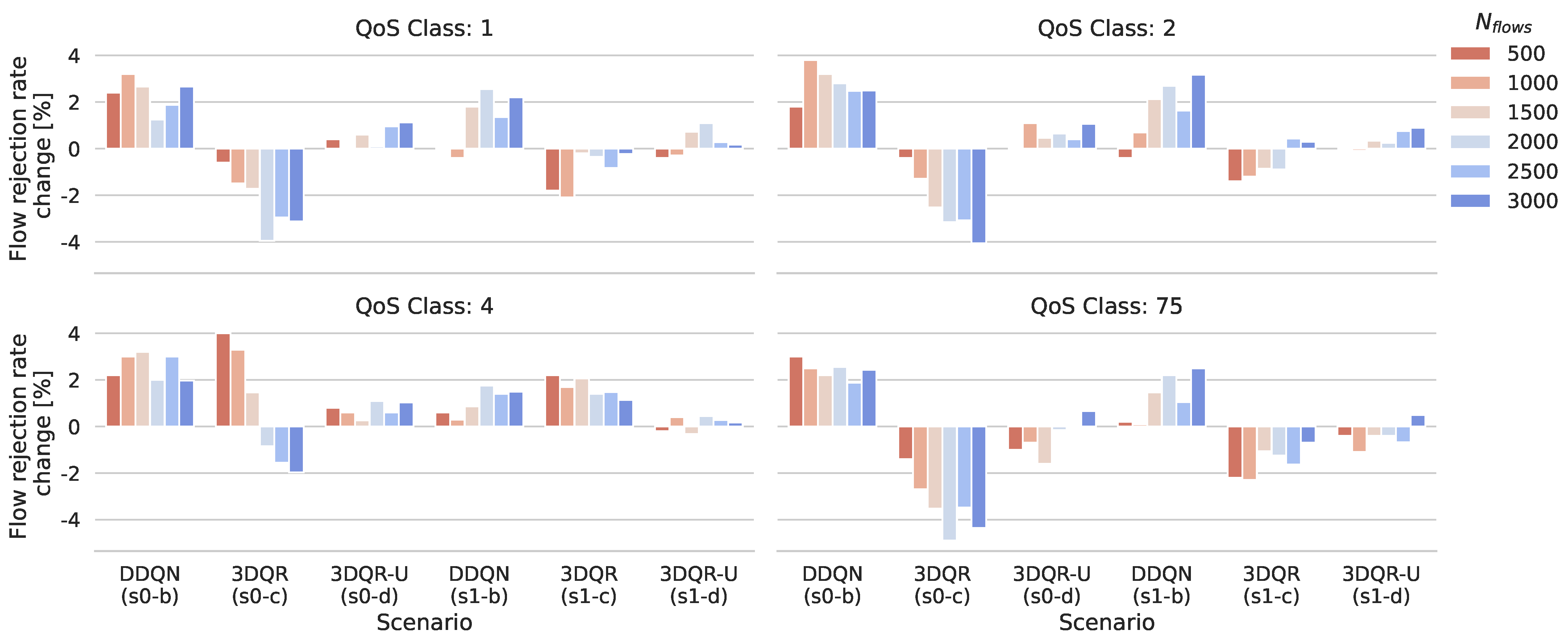
• Performance—showing gains of 3DQR compared to three baseline methods: (i) the most-common SP routing using link delay as the weight metric at both overlay and domain levels, further referred to as H-SP; (ii) a combination of SP for overlay routing and NTNs and classic DDQN for TNs (DNN-based architecture), and 3DQR-Uncoordinated (3DQR-U)—domain DGAs and SP-routing at the overlay level (cf. Section 6.1);
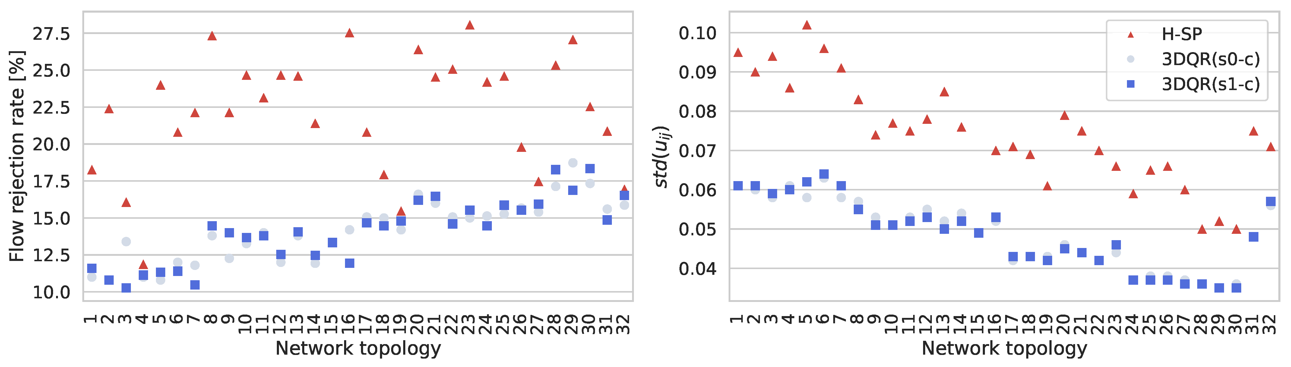
• Transfer capabilities—comprising performance tests of DGAs trained in one topology and operating in previously unseen topologies with different topological properties (cf. Section 6.2);
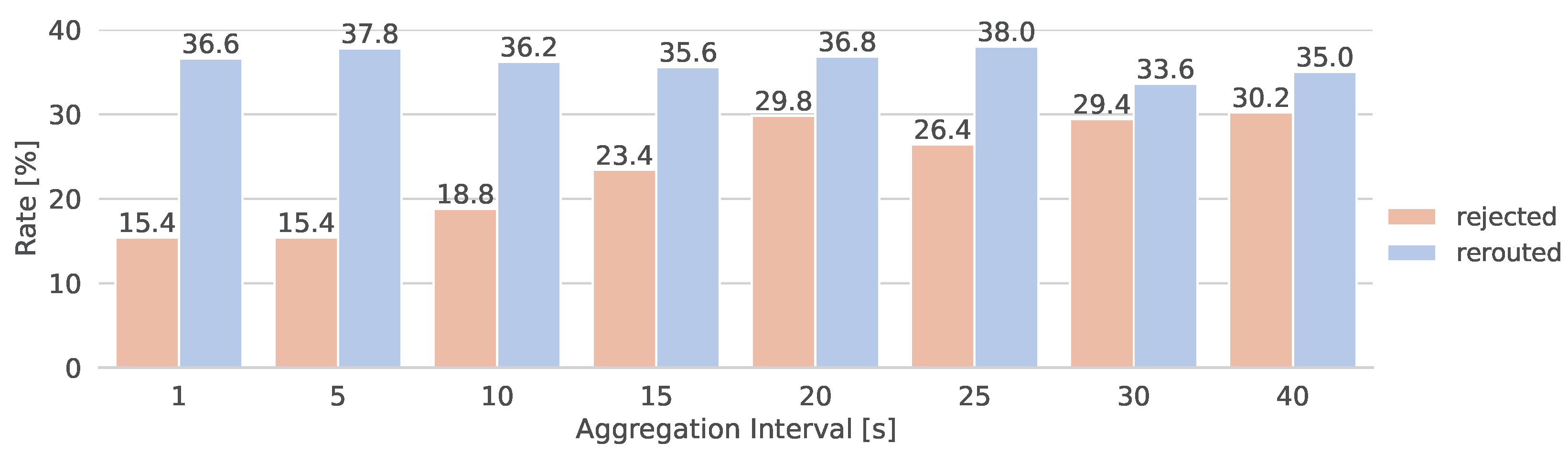
• Aggregation impact—verifying the impact of interval of topology aggregation by GIMMF on 3DQR performance under low traffic load (cf. Section 6.3).

Table 1. Conducted test scenarios. Transfer capabilities are evaluated using models trained in s0-c and s1-c tests.

Test ID	Topology	Algorithm (TN, NTN, TN-NTN)	Scope
s0-a	T1	H-SP	Performance
s0-b		DDQN-SP-SP
s0-c		3DQR
s0-d		3DQR-U
s1-a	T2	H-SP
s1-b		DDQN-SP-SP
s1-c		3DQR
s1-d		3DQR-U
s2-a	T1-T23	H-SP	Transfer
s2-b		3DQR (s0-c)
s2-c		3DQR (s1-c)
s3	T1	3DQR	Topology aggregation interval 1–40 s

Table 1. Conducted test scenarios. Transfer capabilities are evaluated using models trained in s0-c and s1-c tests.

Test ID	Topology	Algorithm (TN, NTN, TN-NTN)	Scope
s0-a	T1	H-SP	Performance
s0-b		DDQN-SP-SP
s0-c		3DQR
s0-d		3DQR-U
s1-a	T2	H-SP
s1-b		DDQN-SP-SP
s1-c		3DQR
s1-d		3DQR-U
s2-a	T1-T23	H-SP	Transfer
s2-b		3DQR (s0-c)
s2-c		3DQR (s1-c)
s3	T1	3DQR	Topology aggregation interval 1–40 s

3DQR was tested in over 30 different topologies comprising both sparse and dense networks (T1–T32) with TN nodes located within western and central Europe. The training and performance evaluation (s0-x, s1-x) were conducted in reference topologies comprised of two TN graphs (32 nodes—50% relays, 25% gateways, and 25% gNodeBs) with average node degrees equal to four (T1) and seven (T2); and (ii) two NTN graphs—subsets of Starlink satellite constellations containing 32 nodes (T1) and 24 nodes (T2), both with an average node degree equal to four (fixed due to limited number of optical interfaces onboard LEOs). To verify transfer capabilities, 20 previously unseen topologies were used, each comprising 16–80 TN and NTN nodes with average node degrees of 3–6. The TN-NTN connections are calculated dynamically based on LEOs proximity to the TN gateway and the visibility criterion (elevation ≥ 30°). Domain-level links and FLs have a capacity of 100 and 200 kilounits, respectively, $\delta ={10}^{-8}$, and delay is calculated based on the spatial distance between nodes. For UE-LEO links, the worst-case delay of 13 ms (the largest value at 600 km orbit as indicated by the 3GPP [48]) and PER of ${10}^{-7}$ were adopted. For UE-TN, the Radio Access Network (RAN) delay of 2 ms and $\delta ={10}^{-8}$ were assumed.

Finally, the adopted QoS classes of arriving flows correspond to expected NTN-based services (cf.

Table 2. QoS profiles used for evaluation (based on [48]).

5QI	PDB [ms]	PER	GFBR	MFBR	QF	Example Service
1	100	10−2	75	150	0.3	Conversational voice
2	150	10−3	2000	5000	0.5	Conversational video
4	300	10−6	1000	2000	0.8	Non-conversational video (buffered streaming)
75	50	10−2	500	1000	0.9	A2X messages, aircraft telemetry

). The arriving flows have a duration of 0.5 to 20 min (generated randomly with uniform distribution) and an equal rate per-QoS class (25% each). In each test, an equal number of flows per domain was generated, i.e., $1/3$ inter-domain flows and $2/3$ intra-domain flows (equal portions for TN and NTN segments).

To set up the DRL models, tests were conducted to fine-tune the network architectures and hyperparameters (e.g., k, $\tau$, $\gamma$) to maximise the models’ performance. As a result, the following configuration was derived for DQRs/M-QR and DGAs: $k=8$, $\gamma =0.85$, $\tau ={10}^{-2}$, ${ϵ}_{min}=0.01$, ${ϵ}_{decay}=0.995$, $N=16$, $\left|t\right|=4$, and a learning rate of ${10}^{-4}$. The DGA Q-networks comprise six passes in the MPNN, GAP with MLP (64 hidden neurons and ReLu activation) as a gate function computing attention scores, and one-neuron LL for the compression. The DDQN architecture (s0-b, s1-b) comprises four LLs: 64, 32, 16, and 1 output neurons. GIMMF aggregates the topology for a 5 s window and provides the topological prediction for another 5 s (10 s into the future). In the 3DQR case, the input size equals the number of node and edge features, while in the DDQN case, the input size equals the number of node and edge features multiplied by the number of graph links.

6.1. Performance

To evaluate the performance, the impact of the algorithms on network availability and load distribution is assessed. To this end, two metrics are considered: flow rejection rate (fraction of rejected flow allocation requests) and the standard deviation of link utilisation $std\left(u_{ij}\right)$ expressing the overall imbalance of traffic across all links in a time step. For each test case, the agents were trained in low-traffic environments for 200 episodes lasting 0.5 h each (500 flow requests per episode—$N_{flows}=500$) and the models were chosen that accumulated the highest aggregate episodic reward. The respective training curves for the 3DQR model are shown in Figure 6.

For both scenarios, the model tends to reach satisfactory reward values after about 100 training episodes. For the s1-c scenario, sudden performance degradation can be observed that might have been caused by over-training (due to the smaller state space in the NTN domain). Nonetheless, the model is able to recover after ≈40 episodes to a decent performance. The disproportions across domains and scenarios are caused by different network topologies, the number of flow rerouting operations, and rerouted flow types (inter-/intra-domain, QoS class).

Based on the aggregate reward, the models that performed the best in their respective environments were selected. For further evaluation, the models were tested against the increasing network load, up to $N_{flows}=3000$, which corresponds to a highly congested network. The results for the best models are shown in Figure 7. First, 3DQR yields a substantial decrease in flow rejection rate compared to H-SP routing for a medium network load and higher ($N_{flows}\ge 1000$). Starting with ≈2% (s0-c, $N_{flows}=1000$), the reduction reaches up to ≈13.5% (s0-c, $N_{flows}=3000$). This is due to the ability of consecutive intra-domain and inter-domain optimisation, which allows for offloading feeder links and better exploiting both ISLs and TN infrastructure. This allows 3DQR to allocate the flows evenly across the available links and minimise the risk of congestion. A performance drop can be observed for lower network loads. This is caused by the number of candidate paths each router processed during the flow allocation. Increasing the number of candidate paths increases the potential length of individual network paths (both domain and overlay level), at the same time impacting the overall delay and packet error rate (leading to rejections caused by exceeding the maximum thresholds, i.e., PDB or PER). Nonetheless, the observed degradation is rather small (lower than 2%) and can be potentially mitigated by reducing the number of evaluated candidate paths. Figure 7 also outlines the performance of a combined DNN-based DDQN with H-SP routing and 3DQR-U, where both fail to provide satisfying results. Using the foremost increases the rejection rate up to ≈10%, which indicates overall poor reasoning capabilities and difficulties in converging in the changing network conditions. Regarding 3DQR-U, it yields comparable results to H-SP routing, but at the same time, it improves the load distribution in the network (see further). Nonetheless, 3DQR provides much better results with a minimal increase in complexity, thus emphasising the importance of overlay level TE in the concept. Overall, it must be emphasised that 3DQR provides stable performance regardless of the network load, thus addressing one of the critical issues of DRL-based approaches, i.e., poor performance and unpredictable behaviour in the previously unseen states. 3DQR via mechanisms of MPNN and GAP (cf. Section 5.3) can overcome this problem by first extracting the key features out of the network graph and then appropriately scaling the node features according to their importance, i.e., the risk of causing congestion in the network.

The second optimisation target for 3DQR is to prioritise the most advantageous QoS classes (i.e., with the highest QF, cf. Table 2). Figure 8 and Figure 9 show the QoS class rejection rate for each algorithm and traffic load and gains compared to the baseline H-SP routing. First, 3DQR enables prioritisation of the most important 5QI class 75, reducing the drop rate in almost every case up to 4.5% in the congested scenario; however, this occurs at the cost of class 4 (total increase up to 4.5%). QoS class 4, however, consumes the most bandwidth across the classes—it is prone to rejection due to occasional congestions (e.g., due to topological reasons, as it can be observed for s0-c and $N_{flows}=2000$). Moreover, the drop rate for the remaining classes is significantly lower and increases with the number of flow requests.

The second major goal of 3DQR is to load balance the traffic to improve resource utilisation, especially ISLs and FLs. Figure 10 shows the distributions of $std\left(u_{ij}\right)$ obtained from the environment during a single episode (aggregate of all segments).

First, 3DQR enables a decrease in the mean $std\left(u_{ij}\right)$, which corresponds to better flow allocation decisions during the episodes (cf.

Table 3. The mean ($\mu$) of $std\left(u_{ij}\right)$ in the best episode (aggregate over domains) and change $\Delta$ compared to the baseline scenario (the lower, the better).

${\mathbf{N}}_{\mathbf{flows}}$	Test	s0-a	s0-b	s0-c	s0-d	s1-a	s1-b	s1-c	s1-d
1000	$\mu$	0.067	0.06	0.044	0.063	0.062	0.065	0.059	0.062
	$\Delta$[%]	-	−11.7	−52.3	−6.3	-	4.6	−5.1	0.0
2000	$\mu$	0.072	0.065	0.048	0.069	0.069	0.073	0.067	0.07
	$\Delta$[%]	-	−10.8	−50.0	−4.3	-	5.5	−3.0	1.4
3000	$\mu$	0.075	0.067	0.051	0.072	0.073	0.077	0.07	0.073
	$\Delta$[%]	-	−11.9	−47.1	−4.2	-	5.2	−4.3	0.0

). For the sparse network, the 3DQR enables up to 52% better distribution of traffic compared to H-SP routing (s0-c). It must be noted that for dense network deployment (s1-c), the gains are consistently lower, but the impact is, respectively, lower. This is caused by the much larger average degree of the network, which leads to evaluating by M-QR multiple shortest paths with a large portion of common links. A potential solution would be to search for the shortest node-disjoint paths to minimise this phenomenon and improve the performance. 3DQR-U, on the other hand, provides consistent gains oscillating around 4–6% for sparse comparable results to H-SP routing for dense networks. A similar trend can be observed for the classical DNN-based DDQN, which indicated the issues of the model to converge in a vast state space. Finally, as shown in Figure 10, 3DQR features lower values of 25th and 75th percentiles for both sparse and dense network scenarios. In the optimal case, the Inter-Quartile Range of $std\left(u_{ij}\right)$ and mean value equal 0. While this is unachievable in real-life networks, 3DQR features $std\left(u_{ij}\right)$ promising values (s0-c).

6.2. Transfer

Here, an attempt to verify the ability of 3DQR to generalise and its reasoning capabilities during the operation in previously unseen topologies is performed. To this end, selected were the best-performance models trained in the T1 and T2 topologies (cf. Section 6.1) and the agents were transferred to over 30 different topologies comprising 16–80 NTN nodes, 32–80 TN nodes, and an average node degree ranging from three to six (sparse to dense network). Also, T1 and T2 topologies were included in the tests to check how well the models native to the environment behave, compared to the transferred ones. Each test consisted of 1500 flow allocation requests with the same configuration described above. The performance comparison is shown in Figure 11.

First, it can be observed that both of the trained models yield outstanding performance in the vast majority of the considered scenarios, decreasing the flow rejection rate (up to 14%) and improving the load distribution (up to ≈50% reduction in $std\left(u_{ij}\right)$). Only in four cases was the rejection rate comparable to H-SP routing case, which regarded tests in highly sparse topologies (i.e., node degree equal to three and a small number of TN/NTN nodes) that effectively limited the agents’ ability for routing improvements (despite the load distribution gains retained across setups, the congestion occurred). Finally, a very similar performance can be observed for s1-c and s0-c models operating in the T1 and T2 topologies, which further emphasises 3DQR generalisation capabilities. The consistent performance across different setups is a result of using an attention mechanism within the agent—the contribution of edge and node utilisation to the candidate paths Q-values are relevantly scaled, which allows the agents to quickly identify the situations with a risk of congestion to avoid allocations to the expiring links.

6.3. Topology Aggregation Interval Impact

The impact of adopting different aggregation time windows by GIMMF for NTN topology provisioning and predictions is shown in Figure 12. The results show both the rejected flow requests due to no viable QoS paths or no connection between the node pair, e.g., due to a disjoint graph. It can be observed that aggregation interval up to 5 s does not substantially impact rejected and rerouted flows. Increasing the duration of the aggregation interval increases the rejection rate up to 30% for 30 s and longer time frames. This phenomenon occurs due to the dynamicity of LEO topology and the progressively decreasing number of available links in the topology used for routing. An increasing aggregation interval decreases the number of viable links for SDNCs to route the traffic flows, ultimately leading to congestions and a higher probability of unavailable QoS-meeting paths or unreachability due to disjoint network graphs, altogether resulting in higher rejection rates. Moreover, adopting long aggregation intervals limits TE possibilities, which further aggravates the performance drop. Therefore, it is advisable to aggregate topology in rather short time windows to mitigate performance drops and, at the same time, conserve SDNCs computational resources that will be spent on frequent rerouting of flows.

7. Considerations and Future Work

The 3DQR algorithm enables improving routing decisions, utilising mobile network’s resources, and decreasing rejection rates for each class. The practical implementation and deployment of the algorithm, however, pose a set of challenges that need to be considered while deploying the concept in carrier-grade networks:

• SDN CP distribution and operations granularity—while hierarchical multi-controller architectures improve the SDN CP scalability, the information exchange needed to establish the E2E paths increases with the degree of distribution. Moreover, it impacts the complexity of an M-SDNC as it needs to synchronise the states and operations of several spatially distant components. Hence, an appropriate deployment strategy and granularity of the distribution need to be adopted, including SDNCs and M-SDNC placement, to avoid large coordination overheads [59].
• Resource utilisation and flow fairness—the allocations with fixed QoS guarantees can lead to resource underspending if the allocated resources differ from the ones actually consumed by flows. To this end, it is vital to properly classify the incoming traffic to minimise this effect and employ advanced monitoring mechanisms to obtain actual resource consumption. Moreover, in the case of excessive allocation by the SDNCs, the DP components would require queue-level mechanisms to enforce flow fairness.
• DRL Performance—the MADRL setup enables decreasing the state space and variability, which allows the agents to converge faster. In certain cases, however, e.g., in sparse topologies, the observable gain from deploying a DRL optimisation agent might be minor due to limited action space. Hence, the 3DQR deployment should also consider the complexity of individual network segments and DGAs deployment costs.
• SLA Violations—due to dynamic conditions, the change of link parameters (e.g., partial ISL occlusion by debris) may result in QoS parameters and SLA violation. Here, allocation itself was focused. However, it is essential to develop monitoring and alerting extensions that allow the tracking of the network status and performing flow rerouting in case of SLA violation risks or mobility events.

8. Summary and Conclusions

This paper presented a novel routing and path allocation framework for future mobile 3D networks called 3DQR. The concept uses hierarchical multi-controller SDN to address key issues of SDN, which involve scalability and interoperability by using operations and metrics abstractions. The framework exploits a MADRL setup for routing based on GNNs and operates on domain and E2E levels, targeting the minimisation of flow rejection and flow rerouting rates and the improvement of load distribution. To improve transferability across different topologies and network configurations, the agent performs the reasoning solely based on the input graph features (node- and link-related SDN DP metrics) and topology prediction data obtained from GIMMF. The conducted evaluation over real and synthetic topologies has proved substantial gains compared to the most common shortest path routing methods regarding traffic distribution (improvement up to 52%) and rejection rate (up to 13.5% smaller) in medium-load to congested network conditions. Finally, considerations regarding deploying the 3DQR concept, possible issues, and perspectives for future improvements have been outlined.

References

1. ITU-R. Future Technology Trends of Terrestrial International Mobile Telecommunications Systems Towards 2030 and Beyond; Report M.2516-0; International Telecommunication Union—Radiocommunication Sector: Geneva, Switzerland, 2022. [Google Scholar]
2. 3GPP. Study on Using Satellite Access in 5G, ver. 16.0.0; Technical Report TR 22.822; 3rd Generation Partnership Project. 2018. Available online: https://portal.3gpp.org/desktopmodules/Specifications/SpecificationDetails.aspx?specificationId=3372 (accessed on 2 March 2025).
3. Guidotti, A.; Vanelli-Coralli, A.; Schena, V.; Chuberre, N.; El Jaafari, M.; Puttonen, J.; Cioni, S. The Path to 5G-Advanced and 6G Non-Terrestrial Network Systems. In Proceedings of the 2022 11th Advanced Satellite Multimedia Systems Conference and the 17th Signal Processing for Space Communications Workshop ASMS/SPSC), Graz, Austria, 6–8 September 2022; pp. 1–8. [Google Scholar] [CrossRef]
4. Tomaszewski, L.; Kołakowski, R.; Mesodiakaki, A.; Ntontin, K.; Antonopoulos, A.; Pappas, N.; Fiore, M.; Mosahebfard, M.; Watts, S.; Harris, P.; et al. ETHER: Energy- and Cost-Efficient Framework for Seamless Connectivity over the Integrated Terrestrial and Non-terrestrial 6G Networks. In Proceedings of the Artificial Intelligence Applications and Innovations. AIAI 2023 IFIP WG 12.5 International Workshops, León, Spain, 14–17 June 2023; Maglogiannis, I., Iliadis, L., Papaleonidas, A., Chochliouros, I., Eds.; pp. 32–44. [Google Scholar] [CrossRef]
5. King, D.; Shortt, K. Time Variant Challenges for Non-Terrestrial Networks; Internet Draft draft-king-tvr-ntn-challanges-00; Internet Engineering Task Force: Wilmington, DE, USA, 2023. [Google Scholar]
6. Ali, I.; Al-Dhahir, N.; Hershey, J. Predicting the Visibility of LEO Satellites. IEEE Trans. Aerosp. Electron. Syst. 1999, 35, 1183–1190. [Google Scholar] [CrossRef]
7. Altamirano, J.C.; Slimane, M.A.; Hassan, H.; Drira, K. QoS-aware Network Self-management Architecture Based on DRL and SDN for Remote Areas. In Proceedings of the 2022 IEEE 11th IFIP International Conference on Performance Evaluation and Modeling in Wireless and Wired Networks (PEMWN), Rome, Italy, 8–10 November 2022; pp. 1–6. [Google Scholar] [CrossRef]
8. Guo, Y.; Lin, B.; Tang, Q.; Ma, Y.; Luo, H.; Tian, H.; Chen, K. Distributed Traffic Engineering in Hybrid Software Defined Networks: A Multi-Agent Reinforcement Learning Framework. IEEE Trans. Netw. Serv. Manag. 2024, 21, 6759–6769. [Google Scholar] [CrossRef]
9. Chen, X.; Ji, Z.; Wu, S.; Jia, H.; Xiao, A.; Jiang, C. A Distributed Routing Algorithm for LEO Satellite Networks: A Multi-Agent Transformer-MIX Learning Approach. IEEE Internet Things J. 2025. Early Access. [Google Scholar] [CrossRef]
10. Liao, H.; Zhang, X.; Zhou, J.; Li, X. Real-Time Routing Design for LEO Satellite Networks: An Enhanced Multi-Agent DRL Approach. In Proceedings of the 2024 IEEE/CIC International Conference on Communications in China (ICCC Workshops), Hangzhou, China, 7–9 August 2024; pp. 547–552. [Google Scholar] [CrossRef]
11. Liu, X.; Chen, A.; Zheng, K.; Chi, K.; Yang, B.; Taleb, T. Distributed Computation Offloading for Energy Provision Minimization in WP-MEC Networks with Multiple HAPs. IEEE Trans. Mob. Comput. 2024. Early Access. [Google Scholar] [CrossRef]
12. Ran, Y.; Ding, Y.; Chen, S.; Lei, J.; Luo, J. Fully-Distributed Dynamic Packet Routing for LEO Satellite Networks: A GNN-Enhanced Multi-Agent Reinforcement Learning Approach. IEEE Trans. Veh. Technol. 2024. Early Access. [Google Scholar] [CrossRef]
13. Ammar, S.; Pong Lau, C.; Shihada, B. An In-Depth Survey on Virtualization Technologies in 6G Integrated Terrestrial and Non-Terrestrial Networks. IEEE Open J. Commun. Soc. 2024, 5, 3690–3734. [Google Scholar] [CrossRef]
14. Bannour, F.; Souihi, S.; Mellouk, A. Distributed SDN Control: Survey, Taxonomy, and Challenges. IEEE Commun. Surv. Tutor. 2018, 20, 333–354. [Google Scholar] [CrossRef]
15. Guo, J.; Yang, L.; Rincon, D.; Sallent, S.; Fan, C.; Chen, Q.; Li, X. SDN Controller Placement in LEO Satellite Networks Based on Dynamic Topology. In Proceedings of the 2021 IEEE/CIC International Conference on Communications in China (ICCC), Xiamen, China, 28–30 July 2021; pp. 1083–1088. [Google Scholar] [CrossRef]
16. Kołakowski, R.; Kukliński, S.; Tomaszewski, L. Hierarchical Deep Reinforcement Learning-Based Load Balancing Algorithm for Multi-Domain Software-Defined Networks. In Proceedings of the 2024 IFIP Networking Conference (IFIP Networking), Thessaloniki, Greece, 3–6 June 2024; pp. 607–612. [Google Scholar] [CrossRef]
17. Geraci, G.; Lopez-Perez, D.; Benzaghta, M.; Chatzinotas, S. Integrating Terrestrial and Non-terrestrial Networks: 3D Opportunities and Challenges. IEEE Commun. Mag. 2022, 61, 42–48. [Google Scholar] [CrossRef]
18. Han, L.; Retana, A.; Westphal, C.; Li, R. Large Scale LEO Satellite Networks for the Future Internet: Challenges and Solutions to Addressing and Routing. Comput. Netw. Commun. 2022, 1, 30–57. [Google Scholar] [CrossRef]
19. Du, P.; Nazari, S.; Mena, J.; Fan, R.; Gerla, M.; Gupta, R. Multipath TCP in SDN-enabled LEO Satellite Networks. In Proceedings of the MILCOM 2016–2016 IEEE Military Communications Conference, Baltimore, MD, USA, 1–3 November 2016; pp. 354–359. [Google Scholar] [CrossRef]
20. Monzon Baeza, V.; Rigazzi, G.; Aguilar, S.; Ferrus, R.; Ferrer, J.; Mhatre, S.; Guadalupi, M. IoT-NTN Communications via Store-and-Forward Core Network in Multi-LEO-satellite Deployments. In Proceedings of the 2024 IEEE 35th International Symposium on Personal, Indoor and Mobile Radio Communications (PIMRC), Valencia, Spain, 2–5 September 2024; pp. 1–6. [Google Scholar] [CrossRef]
21. 3GPP. Study on Satellite Access—Phase 3, ver. 19.2.0. Technical Report TR 22.865. 3rd Generation Partnership Project. 2023. Available online: https://portal.3gpp.org/desktopmodules/Specifications/SpecificationDetails.aspx?specificationId=4089 (accessed on 2 March 2025).
22. Orange. Mobile Network Technology Evolutions Beyond 2030; White Paper; Orange: Paris, France, 2024. [Google Scholar]
23. Yang, Z.; Li, H.; Wu, Q.; Wu, J. Topology Discovery Sub-Layer for Integrated Terrestrial-Satellite Network Routing Schemes. China Commun. 2018, 15, 42–57. [Google Scholar] [CrossRef]
24. Cao, X.; Li, Y.; Xiong, X.; Wang, J. Dynamic Routings in Satellite Networks: An Overview. Sensors 2022, 22, 4552. [Google Scholar] [CrossRef] [PubMed]
25. Korikawa, T.; Takasaki, C.; Hattori, K.; Oowada, H. Time-Topology Routing in 3D Networks. In Proceedings of the 2023 International Conference on Computing, Networking and Communications (ICNC), Honolulu, HI, USA, 20–22 February 2023; pp. 348–352. [Google Scholar] [CrossRef]
26. Kumar, P.; Bhushan, S.; Halder, D.; Baswade, A.M. fybrrLink: Efficient QoS-aware Routing in SDN Enabled Next-Gen Satellite Networks. arXiv 2021, arXiv:2106.07778. [Google Scholar] [CrossRef]
27. Jiang, Y.; Wu, S.; Mo, Q. A Compass Time-Space Model-Based Virtual IP Routing Scheme for NTSN Satellite Constellations. Chin. J. Aeronaut. 2023, 36, 280–288. [Google Scholar] [CrossRef]
28. Yang, Z.; Liu, H.; Jin, J.; Tian, F. A Cooperative Routing Algorithm for Data Downloading in LEO Satellite Network. In Proceedings of the 2021 IEEE 21st International Conference on Communication Technology (ICCT), Tianjin, China, 13–16 October 2021; pp. 1386–1391. [Google Scholar] [CrossRef]
29. Liu, Q.; Li, X.; Ji, H.; Zhang, H. Multi-Path Routing Algorithm with Joint Optimization of Load-Balancing for Cluster-Based Leo Satellite Networks. In Proceedings of the 2023 8th IEEE International Conference on Network Intelligence and Digital Content (IC-NIDC), Beijing, China, 3–5 November 2023; pp. 264–268. [Google Scholar] [CrossRef]
30. Rao, Y.; Wang, R. Multi-Path QoS Routing Using Genetic Algorithm for LEO Satellite Networks. Chin. J. Electron. 2011, 20, 17–20. [Google Scholar]
31. Lian, P.; Yan, F.; Luo, H.; Wang, Z.; Zhang, S. Multicast Source Routing Based on Bloomed Link Identifiers for LEO Satellite Network. In Proceedings of the 2022 IEEE International Conference on Satellite Computing (Satellite), Shenzhen, China, 26–27 November 2022; pp. 13–18. [Google Scholar] [CrossRef]
32. Ventre, P.L.; Tajiki, M.M.; Salsano, S.; Filsfils, C. SDN Architecture and Southbound APIs for IPv6 Segment Routing Enabled Wide Area Networks. IEEE Trans. Netw. Serv. Manag. 2018, 15, 1378–1392. [Google Scholar] [CrossRef]
33. Tang, F.; Mao, B.; Kawamoto, Y.; Kato, N. Survey on Machine Learning for Intelligent End-to-End Communication Toward 6G: From Network Access, Routing to Traffic Control and Streaming Adaption. IEEE Commun. Surv. Tutor. 2021, 23, 1578–1598. [Google Scholar] [CrossRef]
34. Wang, C.; Wang, H.; Wang, W. A Two-Hops State-Aware Routing Strategy Based on Deep Reinforcement Learning for LEO Satellite Networks. Electronics 2019, 8, 920. [Google Scholar] [CrossRef]
35. Tsai, K.C.; Fan, L.; Wang, L.C.; Lent, R.; Han, Z. Multi-Commodity Flow Routing for Large-Scale LEO Satellite Networks Using Deep Reinforcement Learning. In Proceedings of the 2022 IEEE Wireless Communications and Networking Conference (WCNC), Austin, TX, USA, 10–13 April 2022; pp. 626–631. [Google Scholar] [CrossRef]
36. Geyer, F.; Carle, G. Learning and Generating Distributed Routing Protocols Using Graph-Based Deep Learning. In Proceedings of the 2018 Workshop on Big Data Analytics and Machine Learning for Data Communication Networks, Budapest Hungary, 20 August 2018; pp. 40–45. [Google Scholar] [CrossRef]
37. Rusek, K.; Suarez-Varela, J.; Almasan, P.; Barlet-Ros, P.; Cabellos-Aparicio, A. RouteNet: Leveraging Graph Neural Networks for Network Modeling and Optimization in SDN. IEEE J. Sel. Areas Commun. 2020, 38, 2260–2270. [Google Scholar] [CrossRef]
38. Zhuang, Z.; Wang, J.; Qi, Q.; Sun, H.; Liao, J. Toward Greater Intelligence in Route Planning: A Graph-Aware Deep Learning Approach. IEEE Syst. J. 2020, 14, 1658–1669. [Google Scholar] [CrossRef]
39. Dudukovich, R.; Hylton, A.; Papachristou, C. A Machine Learning Concept for {DTN} Routing. In Proceedings of the 2017 IEEE International Conference on Wireless for Space and Extreme Environments (WiSEE), Montreal, QC, Canada, 10–12 October 2017; pp. 110–115. [Google Scholar] [CrossRef]
40. Zhang, S.; Yin, B.; Zhang, W.; Cheng, Y. Topology Aware Deep Learning for Wireless Network Optimization. IEEE Trans. Wirel. Commun. 2022, 21, 9791–9805. [Google Scholar] [CrossRef]
41. Almasan, P.; Suárez-Varela, J.; Rusek, K.; Barlet-Ros, P.; Cabellos-Aparicio, A. Deep Reinforcement Learning Meets Graph Neural Networks: Exploring a Routing Optimization Use Case. Comput. Commun. 2022, 196, 184–194. [Google Scholar] [CrossRef]
42. He, C.; Balasubramanian, K.; Ceyani, E.; Yang, C.; Xie, H.; Sun, L.; He, L.; Yang, L.; Yu, P.S.; Rong, Y.; et al. FedGraphNN: A Federated Learning System and Benchmark for Graph Neural Networks. arXiv 2021, arXiv:2104.07145. [Google Scholar] [CrossRef]
43. Eiza, M.; Raschellà, A. A Hybrid SDN-based Architecture for Secure and QoS Aware Routing in Space-Air-Ground Integrated Networks (SAGINs). In Proceedings of the 2023 IEEE Wireless Communications and Networking Conference (WCNC), Glasgow, UK, 26–29 March 2023. [Google Scholar] [CrossRef]
44. Wei, L.; Shuai, J.; Liu, Y.; Wang, Y.; Zhang, L. Service Customized Space-Air-Ground Integrated Network for Immersive Media: Architecture, Key Technologies, and Prospects. China Commun. 2022, 19, 1–13. [Google Scholar] [CrossRef]
45. Zhang, N.; Zhang, S.; Yang, P.; Alhussein, O.; Zhuang, W.; Shen, X.S. Software Defined Space-Air-Ground Integrated Vehicular Networks: Challenges and Solutions. IEEE Commun. Mag. 2017, 55, 101–109. [Google Scholar] [CrossRef]
46. ONF. OpenFlow Switch Specification, Version 1.5.1 (Protocol Version 0x06); Specification ONF TS-025; Open Networking Foundation: Palo Alto, CA, USA, 2015. [Google Scholar]
47. van Hasselt, H.; Guez, A.; Silver, D. Deep Reinforcement Learning with Double Q-learning. In Proceedings of the 30th AAAI Conference on Artificial Intelligence, Phoenix, AZ, USA, 12–17 February 2015. [Google Scholar] [CrossRef]
48. 3GPP. System Architecture for the 5G System (5GS), ver. 19.2.1. Technical Standard TS 23.501. 3rd Generation Partnership Project. 2025. Available online: https://portal.3gpp.org/desktopmodules/Specifications/SpecificationDetails.aspx?specificationId=3144 (accessed on 2 March 2025).
49. Phemius, K.; Bouet, M. Monitoring Latency with OpenFlow. In Proceedings of the 9th International Conference on Network and Service Management (CNSM 2013), Zurich, Switzerland, 14–18 October 2013; pp. 122–125. [Google Scholar] [CrossRef]
50. Wang, J.; Liu, J.; Guo, H.; Mao, B. Deep Reinforcement Learning for Securing Software-Defined Industrial Networks With Distributed Control Plane. IEEE Trans. Ind. Inform. 2022, 18, 4275–4285. [Google Scholar] [CrossRef]
51. Tang, M.; Cai, S.; Lau, V.K.N. Online System Identification and Control for Linear Systems with Multiagent Controllers Over Wireless Interference Channels. IEEE Trans. Autom. Control 2023, 68, 6020–6035. [Google Scholar] [CrossRef]
52. van Hasselt, H. Double Q-learning. In Advances in Neural Information Processing Systems 23: Proceedings of the 24th Annual Conference on Neural Information Processing Systems, Vancouver, BC, Canada, 6–9 December 2010; Lafferty, J.D., Williams, C.K.I., Shawe-Taylor, J., Zemel, R.S., Culotta, A., Eds.; Curran Associates, Inc.: New York, NY, USA, 2010; Volume 3, pp. 2613–2621. [Google Scholar]
53. Gilmer, J.; Schoenholz, S.S.; Riley, P.F.; Vinyals, O.; Dahl, G.E. Neural Message Passing for Quantum Chemistry. In Proceedings of the 34th International Conference on Machine Learning—Volume 70, ICML’17, Sydney, NSW, Australia, 6–11 June 2017; pp. 1263–1272. Available online: https://dl.acm.org/doi/pdf/10.5555/3305381.3305512 (accessed on 2 March 2025).
54. Lee, J.; Lee, I.; Kang, J. Self-Attention Graph Pooling. arXiv 2019, arXiv:1904.08082. [Google Scholar] [CrossRef]
55. SimPy Documentation. Available online: https://simpy.readthedocs.io/en/latest/ (accessed on 2 March 2025).
56. PyG Documentation—Pytorch_geometric Documentation. Available online: https://pytorch-geometric.readthedocs.io/en/latest/ (accessed on 2 March 2025).
57. Skyfield—Documentation. Available online: https://rhodesmill.org/skyfield/ (accessed on 2 March 2025).
58. CelesTrak: Current Supplemental GP Element Sets. Available online: https://celestrak.org/NORAD/elements/supplemental/ (accessed on 2 March 2025).
59. Gunther, N.J. A Simple Capacity Model of Massively Parallel Transaction Systems. In Proceedings of the 19th International Computer Measurement Group Conference, San Diego, CA, USA, 6–10 December 1993. [Google Scholar]
Figure 1. Overall view of 3DQR concept and interactions across components.
Electronics 14 01045 g001
Figure 2. M-QR/QR and DGA architecture and data flow.
Electronics 14 01045 g002
Figure 3. Path allocation in 3DQR concept.
Electronics 14 01045 g003
Figure 4. Architecture and interactions of DQR/M-QR and DGA (current and target Q-networks and loss function). Domain and overlay identifiers d , ψ are omitted for simplification.
Electronics 14 01045 g004
Figure 5. Complexity comparison of 3DQR, H-SP, and SP routing for different average node degrees.
Electronics 14 01045 g005
Figure 6. Episodic reward obtained by 3DQR model in low-traffic environment: for domain agents TN, NTN and overlay ψ (left); total agents’ reward (right).
Electronics 14 01045 g006
Figure 7. Rejected flows per test setups s0–s1.
Electronics 14 01045 g007
Figure 8. Rejected flows rate for tests per QoS class.
Electronics 14 01045 g008
Figure 9. Change of flow rejection rate per QoS class compared to baseline H-SP routing.
Electronics 14 01045 g009
Figure 10. Standard deviation of utilisation u i j of links per domain (mean marked with red dot) for different loads.
Electronics 14 01045 g010
Figure 11. Performance comparison of H-SP-routing and 3DQR model in terms of flow rejection rate (left) and load distribution (right). Codes 31 and 22 refer to topologies T1 and T2.
Electronics 14 01045 g011
Figure 12. Impact of aggregation interval on flow rerouting and rejection rate.
Electronics 14 01045 g012