MFA-YOLO: Multi-Scale Fusion and Attention-Based Object Detection for Autonomous Driving in Extreme Weather

Abstract

Object detection algorithms are a core technology in autonomous vehicle driving. However, mainstream algorithms still struggle with high missed detection rates and inaccuracies when handling distant, small, or occluded targets, as well as targets that closely resemble the background. These challenges are further exacerbated under extreme weather conditions, leading to even greater recognition inaccuracies. This work addresses these issues through several optimizations, including the development of a module for extracting high- and low-frequency detailed features, a module for capturing vertical and horizontal features, and a hierarchical module that fuses attention mechanisms with convolutional operations. Additionally, the loss function was improved to enhance the algorithm’s focus on difficult samples, thereby increasing its robustness. The proposed algorithm was evaluated on multiple datasets, and the experimental results demonstrate that it outperforms the existing object detection algorithms, delivering superior accuracy and reliability.

1. Introduction

The detection of vehicles and pedestrians using cameras is a critical aspect of object detection in computer vision. This topic has also gained significant attention in various other fields, such as elderly care and unmanned robot delivery. However, in the field of autonomous driving, the speed and accuracy of object detection are held to much higher standards as they directly impact the safety of both pedestrians and drivers. Object detection technology serves as the “eyes” of the vehicle, enabling accurate identification of targets and providing the basis for subsequent automatic control and decision-making processes. In recent years, with the rapid advancements in deep learning—particularly the exceptional performance of convolutional neural networks (CNNs) in computer vision—the capabilities of object recognition technology have steadily improved.

Currently, numerous object detection algorithms have been developed in both academia and industry, which can be broadly categorized into two types: two-stage algorithms and one-stage algorithms. A prominent example of the two-stage approach is the Region-Based Convolutional Neural Network (R-CNN) [1]. An R-CNN first employs selective search to generate candidate regions, which are then fed into a pre-trained CNN for feature extraction. A support vector machine (SVM) is subsequently used to classify each region, followed by border position optimization of the candidate regions. Finally, non-maximum suppression (NMS) is applied to eliminate duplicate bounding boxes, resulting in the final detection output. While the R-CNN approach achieves strong detection accuracy, its computational cost is high and its processing speed is slow due to the need to handle each candidate region individually. Subsequent advancements, such as Fast R-CNN [2], Faster R-CNN [3], Mask R-CNN [4], and DynaMask R-CNN [5], have improved efficiency and accuracy. However, due to their inherent two-stage mechanism, these algorithms struggle to match the speed of one-stage algorithms.

One-stage object detection algorithms bypass the process of generating candidate regions, performing detection directly on the input image. This design typically results in higher detection speed and real-time performance compared to two-stage approaches. Notable one-stage algorithms include the You Only Look Once (YOLO) [6] series and the Single Shot MultiBox Detector (SSD) [7]. It is worth noting that DETR (DEtection TRansformers) [8], based on a Transformer architecture, has garnered significant attention for its end-to-end framework, which eliminates the need for anchor boxes and NMS. The YOLO algorithm divides the input image into grids, performing object detection and bounding box regression within each grid. Its remarkable detection speed makes it particularly well suited for real-time applications. Given the stringent real-time requirements of autonomous driving tasks, the YOLO algorithm is employed to complete target detection in our work. The YOLO series has evolved substantially, progressing from YOLOv2 to YOLOv4 [9,10,11], with each generation contributing notable advancements that have significantly enhanced real-time object detection technology.

Starting with YOLOv5, the YOLO series matured into a widely adopted solution in the industry. From YOLOv5 to YOLOv10 [12,13,14,15,16,17], the series has focused on enhancing computational efficiency, accuracy, and adaptability across various applications. YOLOv5, released in 2020, introduced several key innovations, including the Focus module for efficient feature extraction, CSPNet for improved gradient flow, and advanced data augmentation techniques like Mosaic and MixUp. It also optimized bounding box prediction with CIoU loss and integrated AutoAnchor for better adaptation to diverse datasets. However, YOLOv5 struggles with detecting small targets and handling occlusions effectively. In 2023, YOLOv8 contributed further performance improvements by introducing an anchor-free mechanism and a dynamic label allocation strategy (Dynamic K-Matching) to enhance training efficiency. The updated C2f module improved the feature extraction capabilities, while the SPP-Fast (SPPF) module replaced the original SPP for faster computations. Despite these advancements, YOLOv8 faces limitations, including high hardware requirements, restricted deployment on edge devices, and continued challenges with small targets and imbalanced category distributions. These limitations highlight the need for further optimization to address the demands of diverse real-world applications.

In the second half of 2024, YOLOv11 [18] was released, introducing significant advancements. The C3k2 module replaced C2f in the backbone to enhance performance, while the C2PSA module improved feature extraction through Pointwise Spatial Attention. Depthwise Convolution (DWConv) was incorporated into the detection head, and multiple versions—nano, small, medium, large, and extra-large—were introduced to accommodate diverse applications. The nano version, being lightweight and fast, is ideal for embedded devices, whereas the extra-large version offers high accuracy, making it suitable for tasks such as satellite imaging and industrial defect detection.

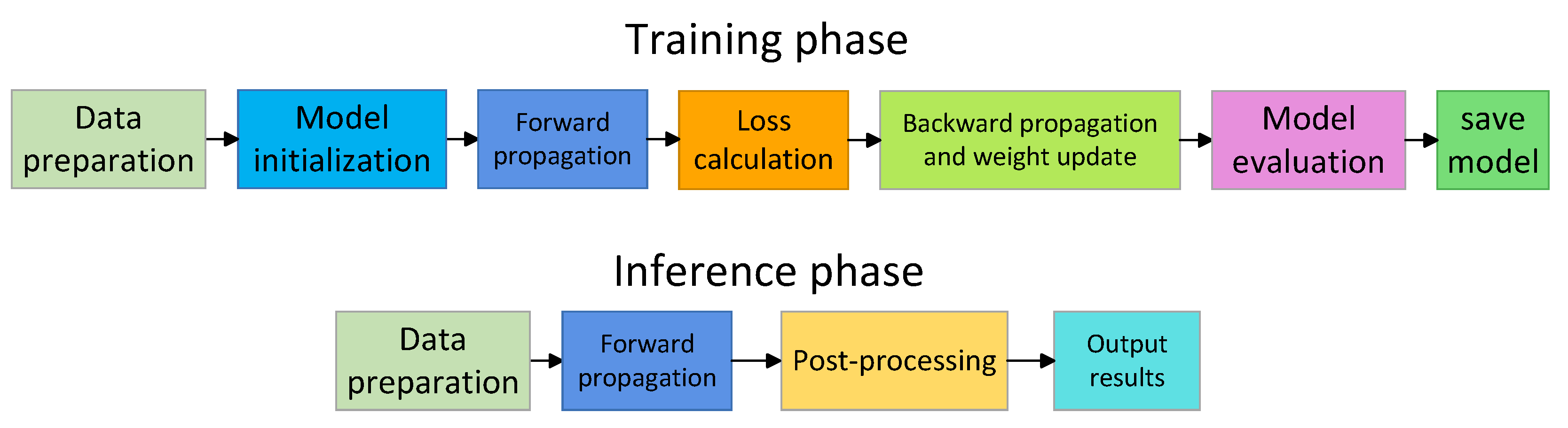
Figure 1 shows the flowchart of the YOLOv11 algorithm, which is divided into two stages: training and inference.

In the training phase, the data preparation module involves loading images and labels from the file system and performing data augmentation, including Mosaic augmentation to enhance small-object detection. After preprocessing, the model initialization module initializes model weights and sets hyperparameters such as the learning rate and optimizer. The process then enters the forward propagation module, where the backbone extracts multi-scale features, the neck fuses feature maps, and the head generates predictions, including category confidence, bounding box parameters, and target confidence. In the loss calculation module, classification loss, bounding box regression loss, and distribution focal loss are computed to obtain the total loss. Subsequently, in the backward propagation and weight update module, gradients are calculated, and the optimizer (e.g., AdamW or SGD) updates the model weights. The model evaluation module assesses the model’s performance on the validation set after each epoch. Finally, when the training reaches the maximum number of epochs, the best model weights are saved.

In the inference phase, the input preparation module preprocesses images by resizing and normalization. During forward propagation, the input image is processed to output the classification, confidence, and bounding box of the detected objects. The post-processing module applies non-maximum suppression (NMS) to remove redundant boxes and retain those with the highest confidence. Finally, the output results module provides the detection results, including target categories, confidence scores, and bounding box coordinates.

The YOLO series is a versatile and widely employed algorithm and framework for object detection, known for its balance of accuracy, speed, and real-time capabilities. While significant research efforts have been devoted to optimizing YOLO for autonomous driving applications, relatively little attention has been paid to addressing its performance limitations under extreme weather conditions. These conditions, such as heavy rain, fog, snow, or low-light scenarios, often exacerbate the challenges of detecting small objects, occluded targets, and distinguishing objects from complex backgrounds. To address these gaps, this paper introduces an improved target detection algorithm based on YOLOv11, specifically designed to perform robustly in extreme weather scenarios. The proposed algorithm incorporates a series of innovative optimizations and enhancements, aimed at overcoming the inherent difficulties in detecting small objects, recognizing occluded targets, and extracting meaningful features from complex images. By addressing these challenges, the improved algorithm advances the performance and reliability of object detection systems in demanding real-world environments.

Our main contributions are summarized as follows:

• To address the challenges in real-world target recognition tasks, such as detecting small targets, handling occluded objects, processing complex images, and managing significant interference noise, we proposed a series of modules, including C3k2-WT, SimSPPF+, and C2PSA-HAFM. These modules are designed to optimize these issues, enabling the model to more accurately capture the features of target objects from complex images and improve the overall algorithm performance.
• To address the issue of sample imbalance within the dataset, we reduced the influence on simple samples while enhancing the focus on difficult ones. By improving the original loss function, we developed the BE-ATFL loss, which performs effectively even when there is a significant disparity in the number of categories. This enhancement optimizes the performance of the target detection algorithm by refining the loss function.
• Building on the proposed improved modules and loss function optimization, we developed a new target detection algorithm, Multi-Scale Fusion and Attention-YOLO (MFA-YOLO). To evaluate its effectiveness, we conducted extensive experiments on multiple datasets. The results demonstrate that MFA-YOLO outperforms other target detection algorithms, showcasing superior practical performance.

2. Related Work

2.1. Real-Time Autonomous Driving

In order to address the issue that traditional detection models tend to detect all appearing objects—including those that are irrelevant to driving safety—Qin et al. [19] proposed a new real-time detection framework, ID-YOLO. This approach simulates the human selective attention mechanism by focusing on salient areas matching the driver’s gaze, and it employs a five-layer architecture to capture objects of different scales more effectively. Nevertheless, the authors primarily evaluated their model on highways, where the detected targets mainly include cars and traffic signs; the performance on urban roads with pedestrians, non-motorized vehicles, and other varied targets remains unclear. Moreover, because ID-YOLO is based on the relatively simple YOLOv3 network structure, its ability to handle highly complex tasks may be limited. Meanwhile, Gao et al. [20] introduced a lightweight detection model based on YOLOX by constructing a simplified path aggregation network (S-PANet). This modification removes redundant bottom fusion paths and retains critical feature information to achieve multi-scale feature fusion at a lower computational cost. Further incorporating the CBAM attention mechanism enhances feature representation and compensates for information loss during simplification. However, while S-PANet reduces the computation and parameter count compared with YOLOX, its detection accuracy declines slightly, indicating a need for further refinements—particularly for smaller targets like pedestrians and cyclists.

A study [21] proposed a real-time target detection system called Edge YOLO, which leverages an Edge-Cloud Cooperation (E-CC) architecture. In this framework, edge devices handle inference while the cloud is responsible for model training and updates, thereby optimizing resource allocation. However, the method’s reliance on stable network conditions makes it vulnerable to bandwidth or latency issues, and its relatively shallow network depth leaves room for improvement—particularly in handling extremely small or densely packed targets. Another investigation [22] explored a multimodal approach that fuses infrared and RGB images, dynamically balancing base-layer and detail-layer information. This strategy effectively enhances detection accuracy in complex environments, but it also increases computational costs and inference time due to the fusion of multiple data streams.

Meanwhile, Lv et al. [23] introduced a multi-target detection algorithm called CMS-YOLO, designed to balance detection accuracy and real-time performance. By refining the network structure, incorporating a multi-scale fusion feature pyramid (MFFPN), and adopting a three-layer joint output approach, CMS-YOLO addresses some of the bottlenecks in conventional YOLO frameworks. Finally, ref. [24] tackled the issue of small-target detection by enhancing the M-ELAN module, integrating the SimAM attention mechanism, and adjusting the parameter ratio between the backbone and neck networks. These modifications aim to improve sensitivity to small objects while maintaining reasonable computational efficiency.

Despite these advances, none of the aforementioned studies explicitly address the challenges posed by extreme weather conditions—such as storms, fog, or snow—which result in limited fields of view, blurred targets, and uneven lighting. Ensuring stable and reliable performance under these adverse conditions remains critical for safe and robust target detection systems.

A recent study [25] introduced a new YOLO-based method to address the challenge of target detection in foggy traffic scenes. This approach builds upon the YOLOv7 architecture, introducing an MSFFA module that fuses features at multiple scales and emphasizes essential regions through an attention mechanism. In addition, a dual-network structure for detection and recovery is employed to mitigate the detrimental impact of fog on object visibility. The experimental results indicate that this method effectively improves detection accuracy by adapting to the reduced contrast inherent in foggy environments. Another work [26] focused on complex snowy conditions and proposed CF-YOLO (cross-fusion YOLO) alongside the creation of a high-quality real snowy object detection dataset, RSOD. By integrating cross-fusion strategies and optimizing feature extraction, this model preserves crucial structural information that is typically degraded by snow, leading to more reliable detection. Although promising, the method assumes that extreme weather primarily affects the target and not the autonomous vehicle’s camera system itself—an assumption that may overlook situations where snow directly degrades sensor performance.

2.2. Small-Target and Difficult-Target Detection

A recent study [27] tackled the challenge of limited receptive fields and restricted feature extraction in conventional CNNs by developing a novel convolutional layer based on wavelet transform. By leveraging the multi-resolution and frequency decomposition properties inherent in wavelet theory, this approach enables more flexible receptive fields and richer feature representations, which have shown promise in semantic segmentation and image classification tasks. Another approach [28] focused on enhancing long-range context modeling by proposing two new spatial pooling methods—strip pooling and mixed pooling—leading to the development of the SPNet architecture, which achieved strong performance on multiple datasets. Building upon the growing emphasis on multi-scale feature learning, a hybrid convolution and attention network (HCANet) [29] combined local feature extraction with global attention mechanisms to tackle hyperspectral image denoising. This approach incorporates multi-scale feedforward networks to capture salient features at varying levels of granularity, resulting in effective noise removal even under complex conditions. Finally, an enhanced feature learning network (EFLNet) [30] was designed to reduce missed and false detections in infrared small-target scenarios by incorporating techniques such as adaptive threshold focal loss (ATFL), Normalized Gaussian Wasserstein Distance (NWD), and Dynamic Head, achieving notable gains in detection performance.

A three-dimensional convolutional network (3D-CNN)-based method called YOLO-3DMM (YOLO 3D Motion Model Network) was proposed in [31] for multiple object tracking (MOT) in traffic scenarios, introducing trajectory non-maximum suppression (TNMS) but exhibiting limited effectiveness for slow or stationary vehicles and for accurately detecting small objects. Another work [32] tackled insufficient feature extraction for small targets by proposing a new algorithm called LTEA-YOLO (Lightweight Transformer and Efficient Attention YOLO), which incorporates a lightweight Transformer module (iRMB) and an efficient attention mechanism (CAPA), although it lacks a robust strategy for targets with extremely few pixels. Further, ref. [33] improved real-time small-target vehicle detection for Unmanned Aerial Vehicle (UAV) scenarios within an IoT context by adding a PrFuFPN feature fusion module and a specialized small-target detection layer, effectively boosting performance.

3. Our Approach

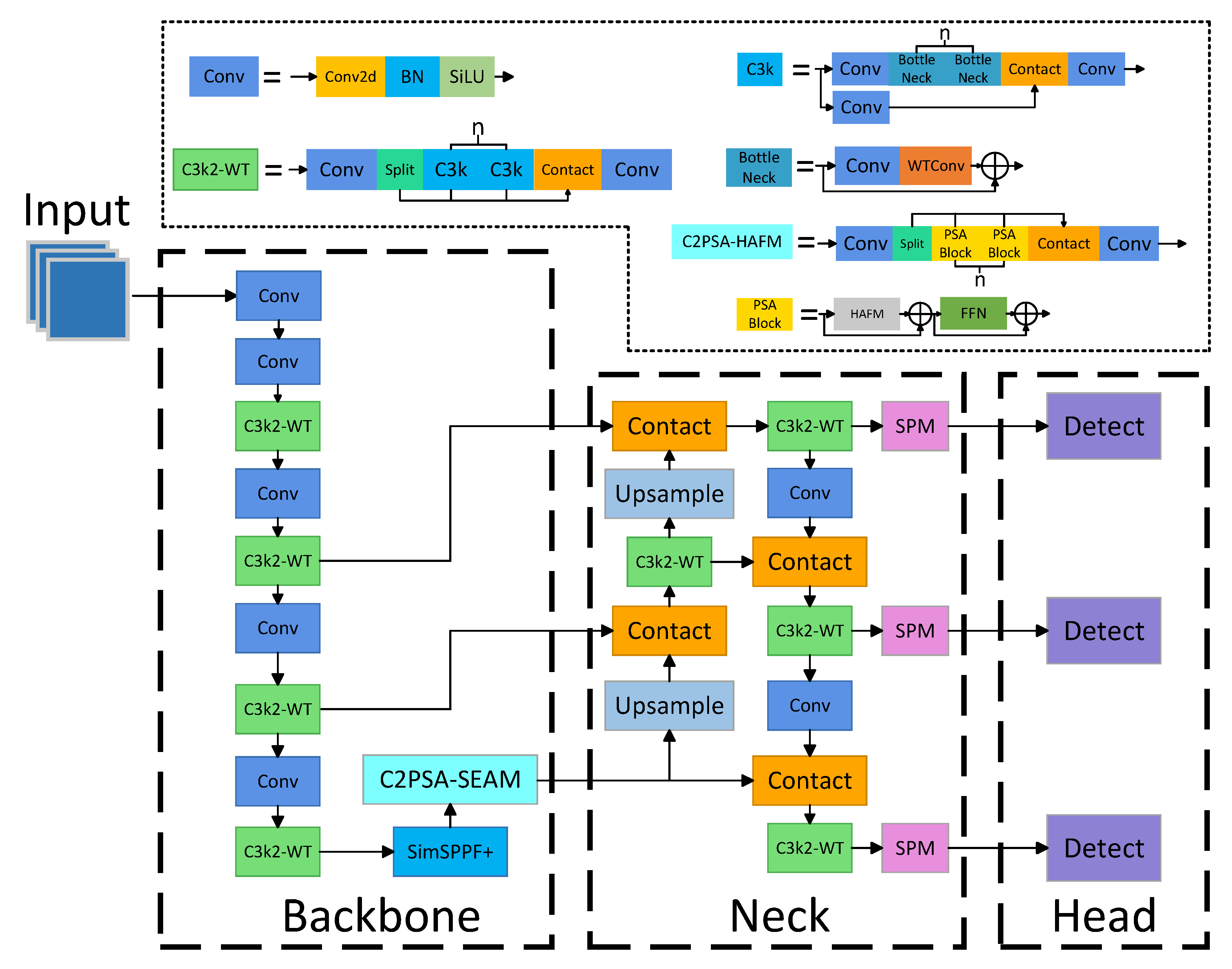
In this section, we provide a detailed explanation of the proposed MFA-YOLO architecture and its key modules. Built upon YOLO v11, MFA-YOLO features a network structure comprising a backbone, a neck, and a detection head, as illustrated in Figure 2.

To address the challenges of poor detection performance for multi-scale targets, the insufficient utilization of semantic information in existing algorithms, and the difficulties of detection under extreme weather conditions, we introduced several improvements to the backbone of the neural network. Specifically, we enhanced the C3k2 module in the original network by integrating wavelet transform, resulting in the C3k2-WT module. This new module employs 2D wavelet transform to decompose image representations at different scales: the low-frequency components extract contour information, while the high-frequency components capture details, edges, textures, and other intricate features. This approach effectively generates richer feature maps even within limited datasets, significantly mitigating the issue of missing detail information in traditional multi-scale target detection models. Additionally, we improved the SPPF module to address the shortcomings of traditional models, particularly their limitations in detecting small targets and achieving a high recall rate. By incorporating the principles of spatial pooling and balancing computational and model complexity, we integrated the strip pooling module (SPM) into the original SPPF module, creating the SimSPPF+ module. This enhanced module features stronger capability for capturing features without significantly increasing computational overhead. Furthermore, we applied SPM before the detection head to refine the screening of feature information, which effectively alleviates the deficiencies of traditional models in small-target detection scenarios. We also enhanced the C2PSA module by replacing its original attention layer with the attention-enhanced HAFM module, resulting in the C2PSA-HAFM module. This new design offers significant advantages in processing complex images and improves overall detection accuracy. Finally, we proposed the bias-enhanced adaptive threshold focal loss (BE-ATFL), an extension of the adaptive threshold focal loss (ATFL), to increase the model’s focus on challenging samples and imbalances. This optimization further enhances the model’s detection capabilities. In the following sections, we will provide a detailed explanation of the C3k2-WT, SimSPPF+, C2PSA-HAFM, and BE-ATFL modules.

3.1. Replace C3k2 with C3K2-WT

Wavelet transform (WT) is a method from the field of signal processing that can effectively increase the receptive field of convolution. We replace some convolutions in the C3K2 module with the WT method, and, based on this, we obtain the C3K2-WT module, as shown in the C3K2-WT module in the upper left corner of Figure 2.

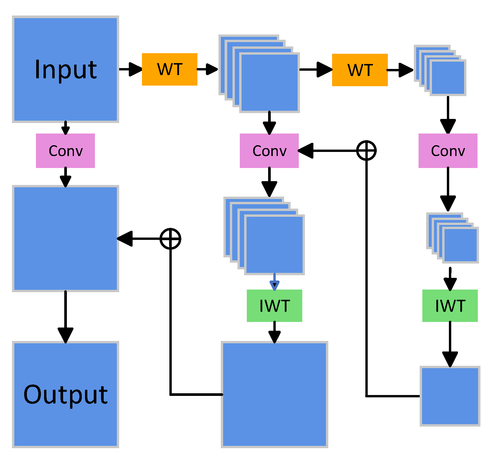
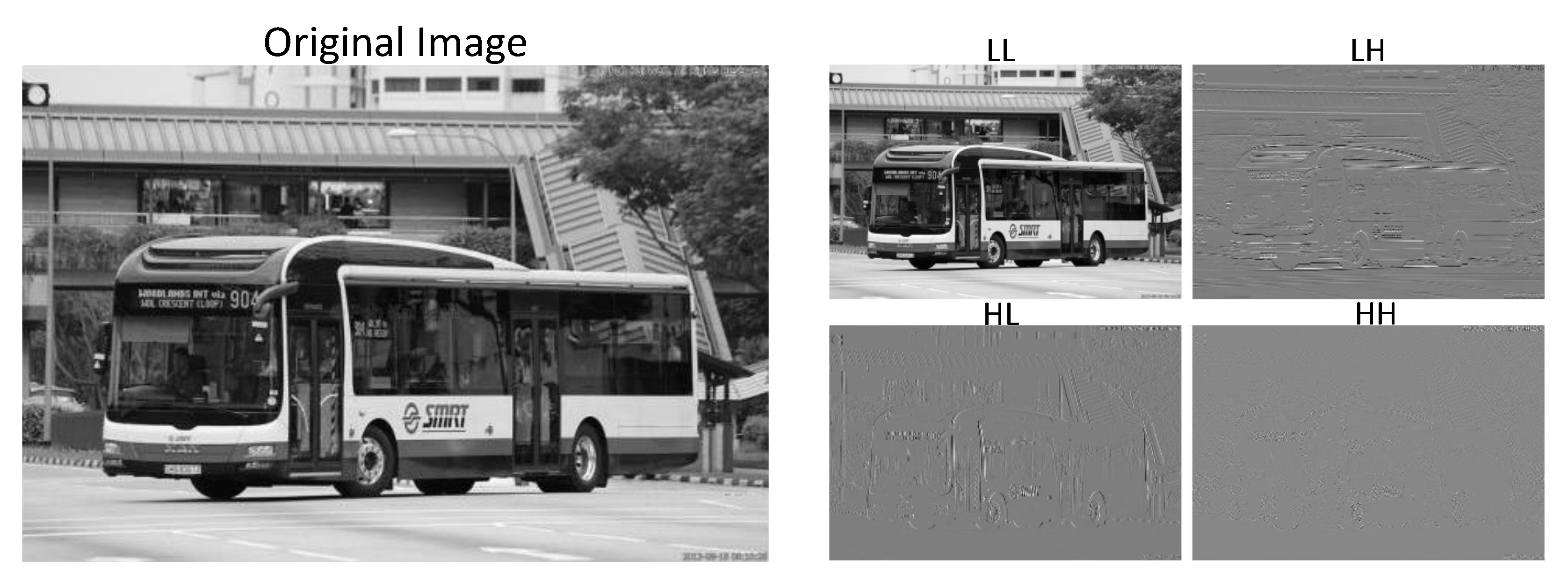
Figure 3 illustrates the structure of the WTConv module. The plus sign in the figure indicates the residual connection. WTConv leverages 2D Haar wavelet transform (WT) to decompose the input into four sub-bands: low-frequency component (LL), horizontal high-frequency component (LH), vertical high-frequency component (HL), and diagonal high-frequency component (HH). Each component is designed to capture specific details at corresponding scales. Specifically, the LL component captures the overall shape and contour, the LH component focuses on horizontal edge information, the HL component extracts vertical edge details, and the HH component highlights diagonal information.

The mathematical principle of WT is as follows. We first assume that the input image is $I(x,y)$, which represents the pixel value of the image in row x and column y. Let g and h represent the low-pass and high-pass filters, respectively, while $\downarrow 2$ denotes the downsampling operation, ∗ denotes convolution operation. The calculation formula for the row low-frequency component $L(x,y)$ and the row high-frequency component $H(x,y)$ is

$$L(x,y)=(I(x,y)\ast g_{row})\downarrow 2,H(x,y)=(I(x,y)\ast h_{row})\downarrow 2.$$

(1)

Next, the row low-frequency component $L(x,y)$ is processed with low-pass and high-pass filtering in the column direction, resulting in $LL(x,y)$ and $LH(x,y)$, respectively. Similarly, the row high-frequency component $H(x,y)$ undergoes low-pass and high-pass filtering in the column direction, yielding $HL(x,y)$ and $HH(x,y)$:

$$\begin{array}{c}\hfill LL(x,y)=(L(x,y)\ast g_{col})\downarrow 2,LH(x,y)=(L(x,y)\ast h_{col})\downarrow 2,\end{array}$$

(2)

$$\begin{array}{c}\hfill HL(x,y)=(H(x,y)\ast g_{col})\downarrow 2,HH(x,y)=(H(x,y)\ast h_{col})\downarrow 2.\end{array}$$

(3)

Figure 4 shows a simple example of an image after WT, and we can clearly see the feature details of its corresponding frequency.

In each level of WT, the image is downsampled (spatial resolution is halved), while the frequency information is decomposed into finer details. By recursively applying wavelet transform (multi-level decomposition) to the low-frequency component, frequency components at multiple scales can be obtained. In WTConv, a small-sized convolution kernel is applied to each frequency sub-band, with typical kernel sizes being 3 × 3 or 5 × 5. Since WT reduces the spatial resolution of each sub-band, these smaller convolution kernels effectively cover a larger receptive field. After completing the convolution operation, the results from each sub-band are fused together using inverse wavelet transform (IWT).

In a 2D WT, the transformation process involves low-pass and high-pass filtering, followed by downsampling. Conversely, the IWT process requires upsampling and inverse filtering. The mathematical principle of IWT begins by performing upsampling and inverse filtering in the column direction to reconstruct the row components:

$$\begin{array}{c}\hfill L(x,y)=\left(LL(x,y)\ast g_{\mathrm{col}}^{\prime }\uparrow 2\right)+\left(LH(x,y)\ast h_{\mathrm{col}}^{\prime }\uparrow 2\right).\end{array}$$

(4)

$$\begin{array}{c}\hfill H(x,y)=\left(HL(x,y)\ast g_{\mathrm{col}}^{\prime }\uparrow 2\right)+\left(HH(x,y)\ast h_{\mathrm{col}}^{\prime }\uparrow 2\right).\end{array}$$

(5)

Then, upsampling and inverse filtering are performed in the row direction to restore the original image:

$$\begin{array}{c}\hfill I(x,y)=\left(L(x,y)\ast g_{\mathrm{row}}^{\prime }\uparrow 2\right)+\left(H(x,y)\ast h_{\mathrm{row}}^{\prime }\uparrow 2\right).\end{array}$$

(6)

where $g^{\prime }$ and $h^{\prime }$ represent the inverse filter kernels of the low-pass filter and the high-pass filter, and $\uparrow 2$ represents the upsampling operation. Since the IWT operation is linear, we can losslessly reconstruct the convolution results into the original space.

In summary, incorporating wavelet convolutions (WTConvs) into a CNN offers two key technical advantages. First, each level of the wavelet transform expands the receptive field size while only slightly increasing the number of trainable parameters. The cascaded frequency decomposition enabled by WT, combined with fixed-size convolution kernels at each level, ensure that the number of parameters grows linearly with the number of levels, while the receptive field expands exponentially. Second, the WTConv layer is specifically designed to capture low-frequency components more effectively than standard convolutions. This is achieved through repeated wavelet decomposition of the low-frequency input, which emphasizes these components and enhances the layer’s corresponding response. By applying compact convolution kernels to multi-frequency inputs, the WTConv layer strategically allocates additional parameters to where they are most impactful. These advantages collectively result in a significant performance improvement regarding CNNs over baseline models.

3.2. Another Approach to Multi-Scale Feature Extraction: Strip Pooling Module

In this subsection, we introduce the strip pooling module (SPM), which is designed to capture long-strip spatial contexts and enhance detection by improving the understanding of textures and structures. In the following subsection, we will demonstrate its integration with the SimSPPF module to create the SimSPPF+ module. Moreover, we applied SPM before the detection head to optimize the screening of feature information and enhance the algorithm’s capability.

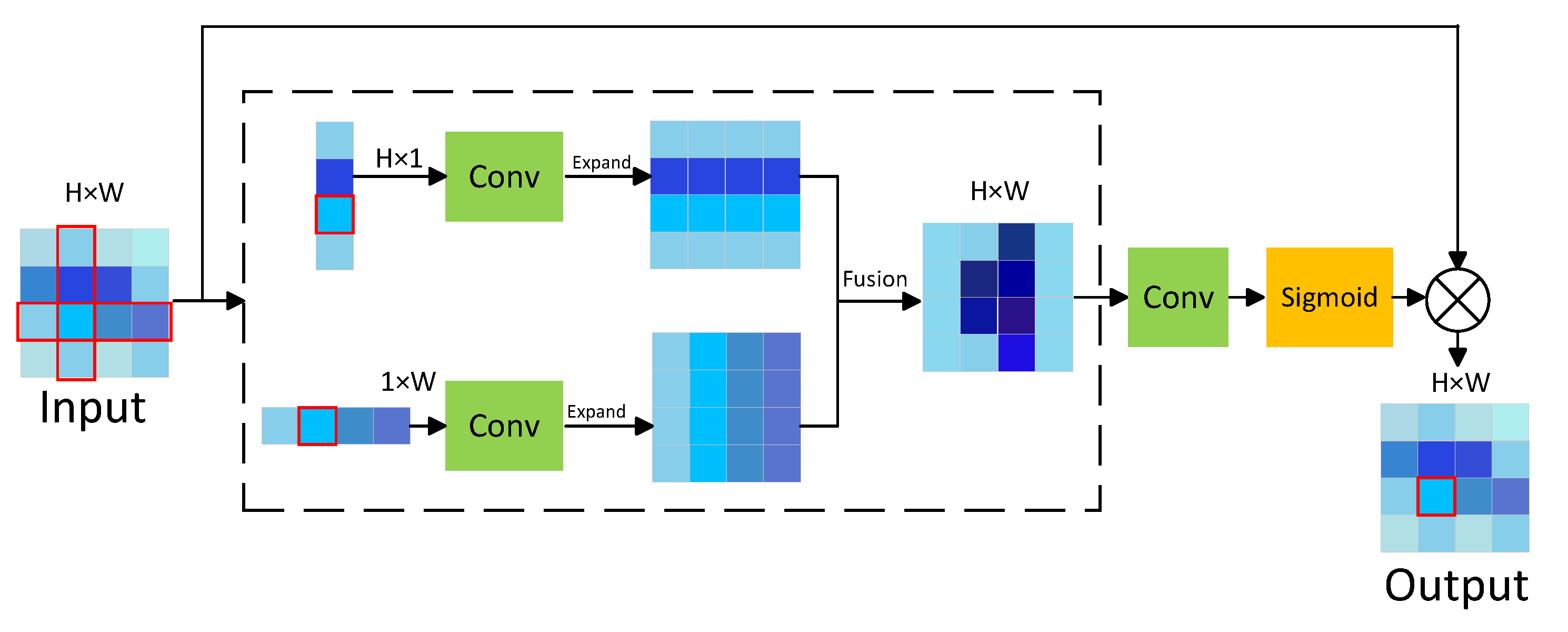
In general, the SPM enhances the representation of both global and local features by capturing long-distance dependencies in two dimensions: horizontal and vertical. As illustrated in Figure 5, when the input is a feature map of size H × W, the SPM extracts features from the map along the horizontal and vertical directions, resulting in a feature map of size H × 1 and another of size 1 × W. Let x represent the input. The output $y^h$ from horizontal strip pooling and $y^v$ from vertical strip pooling can be expressed as

$$y_i^h={\displaystyle \frac{1}{W}}\sum _{0\le j<W}{x}_{i,j},y_j^v={\displaystyle \frac{1}{H}}\sum _{0\le i<H}{x}_{i,j}.$$

(7)

These two feature maps are each processed through a 1 × 1 convolution layer to extract critical information, ensuring that both local and contextual details are captured. After passing through the convolution layer, the feature maps are expanded and fused, resulting in a combined map enriched with global prior information. To further enhance the feature representation, the fused feature map undergoes an additional 1 × 1 convolution and is normalized using a sigmoid function, which balances feature weights and highlights the most relevant features. This refined feature map is then multiplied with the original input, enabling the network to effectively integrate the enhanced global and local features into the final representation. The calculation for the final output features is expressed as follows:

$$\begin{array}{c}\hfill Outpu{t}_{SPM}=x\odot \sigma \left(Conv\left(y\right)\right).\end{array}$$

(8)

where y represents the fused horizontal pooling feature map $y^h$ and vertical pooling feature map $y^v$ and $\mathbf{y}$=$y^h$+$y^v$. $Conv$ represents 1 × 1 convolution. $\sigma$ is the sigmoid function. ⊙ is element-by-element multiplication.

3.3. Replace SPPF with SimSPPF+

The SPP module enhances feature fusion by applying three parallel maximum pooling operations with kernel sizes of 5 × 5, 9 × 9, and 13 × 13. However, this approach is computationally intensive, leading to a significant decrease in the network’s inference speed. To address this issue, the SPPF and SimSPPF modules introduce an optimized method by performing multiple 5 × 5 maximum pooling operations sequentially. Specifically, two consecutive 5 × 5 pooling operations produce results equivalent to a single 9 × 9 operation, while three sequential 5 × 5 operations replicate the effect of a 13 × 13 pooling operation.

Furthermore, the SimSPPF module replaces the SiLU activation function used in SPPF with the ReLU activation function, further streamlining the computation. By adopting the SimSPPF module, we achieved comparable performance to the original SPP module while simplifying the design by standardizing all convolution kernels to three 5 × 5 kernels. This optimization not only reduced computational complexity but also significantly improved the model’s inference efficiency.

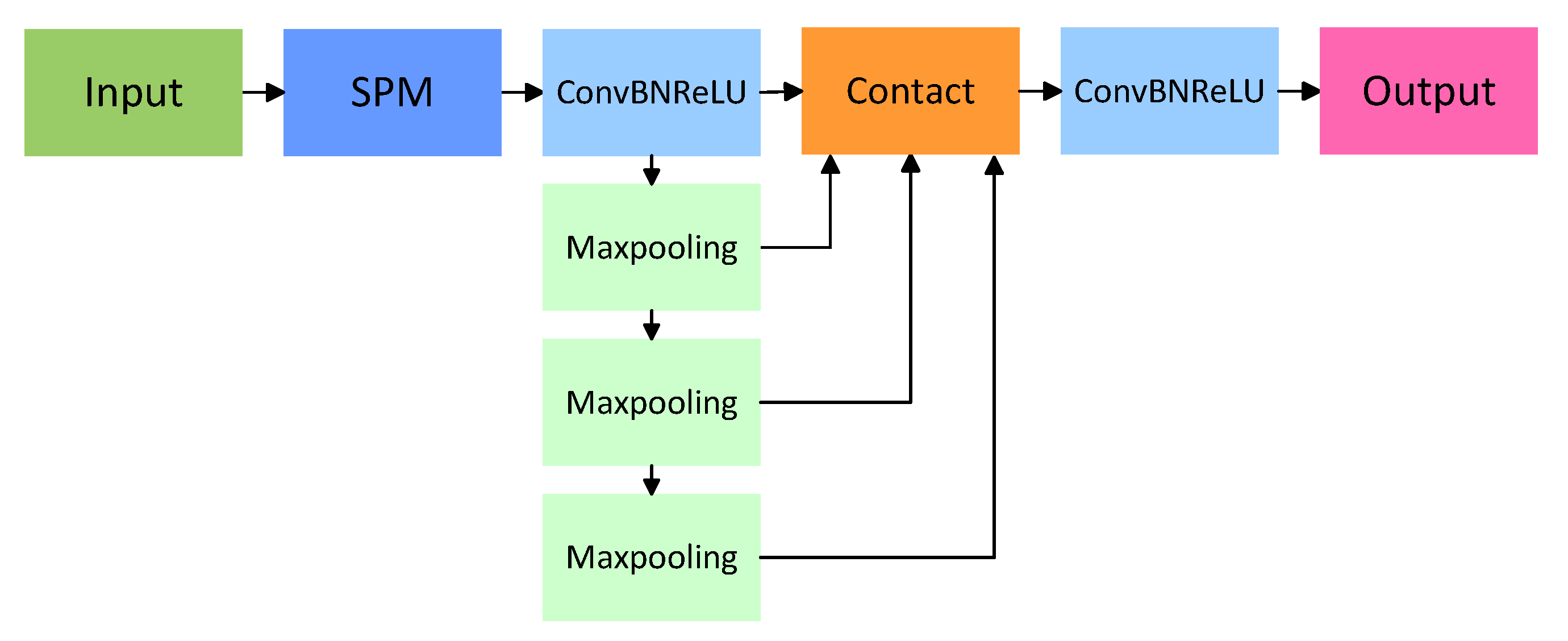
Building on this foundation, we developed the SimSPPF+ module to further enhance the model’s performance. The block diagram of SimSPPF+ is shown in Figure 6. By incorporating an SPM module before the traditional SimSPPF module, the model’s capability to recognize long-strip targets is significantly improved, making it particularly well suited for vehicle detection tasks on roads.

3.4. Replace C2PSA with C2PSA-HAFM

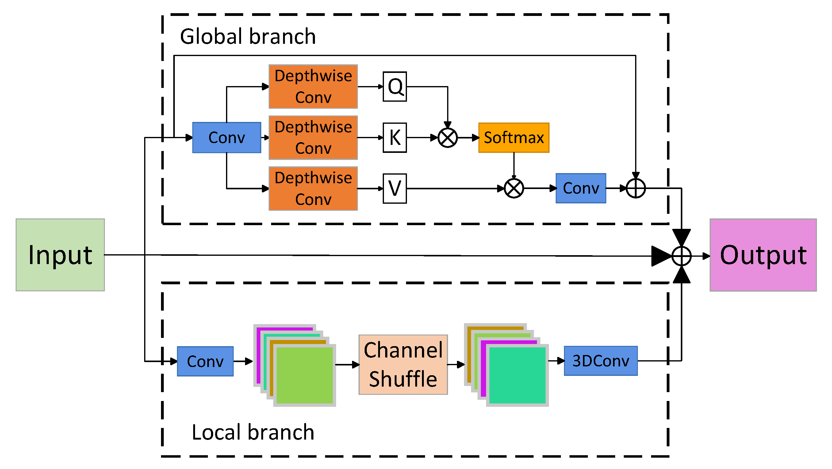
The convolution operation is highly effective at feature perception but often struggles to capture long-range dependencies and global information. To overcome this limitation, the Transformer utilizes an attention mechanism to address these challenges effectively. Building on this concept and incorporating a hierarchical design approach, we propose the Hierarchical Attention Fusion Module (HAFM), which replaces the traditional attention layer in the C2PSA module. The resulting C2PSA-HAFM module significantly enhances the model’s capacity to extract features from complex images and robustly handle challenges such as interference noise.

Figure 7 provides a schematic diagram of the HAFM module. The input is divided into three branches: the local branch $B_{local}$, the global branch $B_{global}$, and itself $B_{self}$. In the local branch, the input is processed sequentially through 1 × 1 convolution, channel shuffle, and 3 × 3 × 3 convolution to produce the output $B_{local}$. In the global branch, the input tensor is transformed through 1 × 1 convolution and 3 × 3 depthwise convolution to generate the query (Q), key (K), and value (V). These components (Q, K, and V) are combined with the original input using an attention mechanism followed by a 1 × 1 convolution to produce the output $B_{global}$. The mathematical expression of the attention is

$$\begin{array}{c}\hfill Attention(Q,K,V)=softmax\left({\displaystyle \frac{Q{K}^T}{\sqrt{d_k}}}\right)V\end{array}$$

(9)

Additionally, in this module, the activation function was changed from SiLU to the GELU activation function, which is better suited for the attention mechanism. Finally, the outputs from the local branch, global branch, and the original input are summed to generate the final output of the HAFM module as follows:

$$\begin{array}{c}\hfill Outpu{t}_{HAFM}=B_{self}+B_{local}+B_{global}\end{array}$$

(10)

By integrating the HAFM module into the C2PSA framework, we introduce the C2PSA-HAFM module, as shown in the upper right corner of Figure 2. This enhanced module achieves a hierarchical combination of global and local features, as well as the input itself, resulting in a significant performance boost, particularly for complex images and those affected by high levels of noise interference.

3.5. Improvement of Loss Function

In small-object detection, the target occupies a small proportion of the image while the background dominates, making it easier for the network to focus on learning background features while neglecting the target’s characteristics. Traditional loss functions struggle to address this imbalance effectively, necessitating improvements to encourage the model to prioritize the features of small targets.

Adaptive threshold focal loss (ATFL) was developed to dynamically balance the contributions of target and background features. Building on this, we introduced further enhancements and proposed the bias-enhanced adaptive threshold focal loss (BE-ATFL) function. The mathematical expression of BE-ATFL is as follows:

$$\begin{array}{cc}\hfill {\mathcal{L}}_{\mathrm{BE}\text{-}\mathrm{ATFL}}& =\left\{\begin{array}{cc}-\left[{(\lambda -p_t)}^{-ln\left(p_t\right)}+\beta b_t^{\theta }\right]log\left(p_t\right),\hfill & p_t\le 0.5\hfill \\ -\left[{(1-p_t)}^{-ln\left(p_t\right)}+\beta b_t^{\theta }\right]log\left(p_t\right),\hfill & p_t>0.5\hfill \end{array}\right.\hfill \end{array}$$

(11)

Here, p represents the predicted probability, and y represents the true label. When $y=1$, $p_t=p$; otherwise, $p_t=1-p$. $\lambda$ is a constant that controls the weight range of the modulation factor. $b_t=|p_t-y|$ represents the absolute error between the predicted probability $p_t$ and the true label y. $\beta$ denotes the bias weighting factor, which determines the influence of the bias $b_t$, while $\theta$ serves as the power exponent of the bias, controlling the nonlinear adjustment of the bias term.

Compared with the basic ATFL loss function, the BE-ATFL loss function introduces an additional bias term $\beta b_t^{\theta }$. For low-confidence samples $(p_t\le 0.5)$, the modulation factor ${(\lambda -p_t)}^{-ln\left(p_t\right)}+\beta b_t^{\theta }$ incorporates the prediction bias $b_t$ to further increase the weight of difficult samples with large $b_t$, thereby enhancing the optimization of these challenging cases. For high-confidence samples $(p_t>0.5)$, the modulation factor ${(1-p_t)}^{-ln\left(p_t\right)}+\beta b_t^{\theta }$ reduces the weight of simpler samples with small $b_t$ through bias control while ensuring adequate focus on difficult cases.

For instance, small targets typically occupy fewer pixels on the feature map, making their prediction prone to larger errors (large bias $b_t$). Similarly, samples near the boundary between target and background areas are often ambiguous, also resulting in larger prediction biases $b_t$. The inclusion of the bias term assigns higher weights to these samples with significant deviations, improving the model’s ability to detect small objects and boundary samples. The bias weight is seamlessly integrated into the original modulation factor without compromising the core idea of the original formula. This enhancement makes the model more flexible and effective in handling complex data, such as class imbalance and samples with varying levels of difficulty.

4. Experiment

4.1. Dataset

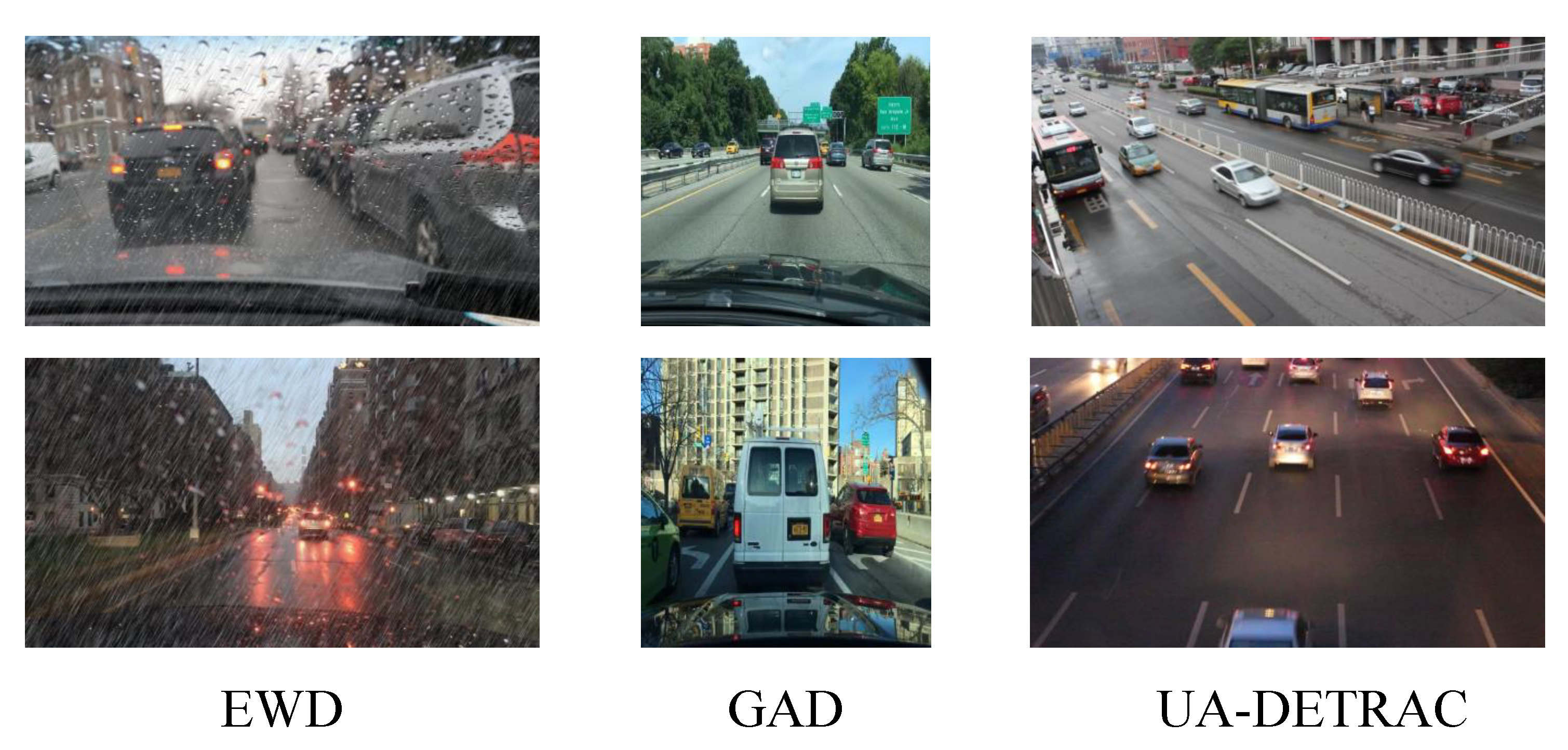
To evaluate the effectiveness of the proposed algorithm under extreme weather conditions, we conducted experiments on the EWD dataset. To further assess its performance in other scenarios, we included the GAD dataset, which focuses on common autonomous driving environments, and the UA-DETRAC dataset, designed for road monitoring from a bird’s-eye view. These diverse datasets enabled us to test the robustness and generalization capabilities of the algorithm across varying conditions. For all experiments, the datasets were split with 80% of the data used for training and 20% for validation.

The EWD dataset is specifically developed for autonomous driving in extreme weather conditions. Most images are captured by a forward-facing camera on vehicles, with a smaller portion taken by side-facing cameras. The primary setting comprises urban roads in rainy weather, with images taken during both day and night. The dataset consists of 3500 labeled images, annotated with seven categories: bike, bus, car, motor, person, rider, and truck.

The GAD dataset is a normal autonomous driving dataset that includes urban and rural road environments, capturing both daytime and nighttime scenarios. It contains 9547 labeled images with ten annotated categories: bicycle, bus, car, motorcycle, pedestrian, rider, traffic light, traffic sign, train, and truck.

The UA-DETRAC dataset is a specialized dataset for vehicle recognition from a surveillance perspective. Unlike the EWD and GAD datasets, it focuses on vehicles captured from a bird’s-eye view. Although the dataset contains a large number of images due to the size of the full dataset, which makes training very time-consuming, we selected only 6249 images for training, with annotations for four vehicle categories: van, truck, bus, and car.

Figure 8 presents some simple sample images from the three datasets mentioned above. The EWD dataset is used for driving in extreme weather with reduced visibility, the GAD dataset is for normal driving conditions (day and night), and the UA-DETRAC dataset monitors vehicles from a bird’s-eye view. These three datasets correspond to three distinct scenarios.

4.2. Experimental Setup

The improved model is implemented using the PyTorch 2.0.0 framework on a system running Windows 11, equipped with an NVIDIA RTX 3080 GPU (NVIDIA Corporation, Santa Clara, CA, USA). The Adam optimizer is used, with an initial learning rate set to 0.001 and a batch size of 16. The input image size is 640 × 640, and the model is trained for a total of 300 epochs. Mosaic data augmentation is disabled 10 epochs before the end of training. To ensure fairness in the experimental comparisons, all algorithms in this paper were trained using the same hyperparameters and dataset as described above. Neither MFA-YOLO nor any of the comparison algorithms utilized pre-trained models; all training was conducted from scratch.

Before training begins, data preprocessing is applied to the dataset. This paper employs various data cleaning and data augmentation techniques to improve the model’s generalization ability and robustness. First, through random rotation and flipping, the model can adapt to different viewpoint changes. Additionally, color transformation techniques, by randomly adjusting brightness, contrast, saturation, and hue, enhance the model’s ability to adapt to different lighting conditions, which helps to improve performance in overly bright or dark lighting scenarios. Image cropping and resizing, by randomly cropping and adjusting the image size, strengthen the model’s robustness to changes in position and size. To improve the algorithm’s performance in noisy and low-quality images, data augmentation also includes the addition of Gaussian noise and the application of Gaussian blur, which aid in enhancing the recognition of motion-blurred targets. Furthermore, translation transformation, by randomly shifting the target’s position, is another common data augmentation strategy. To prevent overfitting, the CutOut technique is used to randomly block out image regions, forcing the model to focus on other features. MixUp, by linearly combining two images with a weight, improves the model’s ability to learn diverse features. Mosaic stitching multiple images together further enriches the data diversity. By comprehensively applying these data preprocessing methods during training, MFA-YOLO is able to maintain high detection performance across various complex scenarios. In the training process, all the models applied the above-mentioned data preprocessing techniques.

4.3. Evaluation Indicator

To comprehensively evaluate the performance of the object detection model, three primary metrics are utilized: precision (P), recall (R), and mean average precision ($mAP$).

Precision (P) measures the proportion of true positives among all positive predictions, reflecting the model’s ability to avoid false positives. Recall (R) evaluates the proportion of true positives correctly identified, showing how well the model captures relevant instances and minimizes false negatives. Mean average precision ($mAP$) is a key metric in object detection that assesses overall model performance by averaging the precision for each object class. A higher $mAP$ indicates better detection accuracy. These metrics together provide a solid evaluation of the model’s performance across different scenarios, calculated using the following formulas:

$$\begin{array}{c}\hfill P={\displaystyle \frac{TP}{TP+FP}},\end{array}$$

(12)

$$\begin{array}{c}\hfill R={\displaystyle \frac{TP}{TP+FN}},\end{array}$$

(13)

$$\begin{array}{c}\hfill \mathrm{mAP}={\displaystyle \frac{{\sum }_{n=1}^{M}A{P}_n}{M}}.\end{array}$$

(14)

Here, $TP$ (true positive) refers to correctly identified objects, $FP$ (false positive) represents incorrectly predicted objects, and $FN$ (false negative) indicates missed objects. M represents the total number of classes in the object detection task, while $A{P}_n$ denotes the average precision for the n-th class.

4.4. Performance Comparison

In order to validate the effectiveness of the proposed algorithm, we conducted experiments using three datasets. The performance of our algorithm was compared against several cutting-edge object detection methods, including YOLOv8, Faster R-CNN, SSD, and RT-DETR. The experimental results are summarized in

Table 1. Comparison of different algorithms on the EWD dataset.

Algorithm	Precision	Recall	mAP
MFA-YOLO (Ours)	72.2	62.5	63.9
YOLOv11	65.3	54.7	56.1
YOLOv10	61.8	52.2	54.2
YOLOv9	61.2	52.0	51.6
YOLOv8	62.0	52.5	52.8
YOLOv5	59.9	51.6	50.6
Faster R-CNN	56.2	49.8	48.7
SSD	55.4	48.8	47.2
RT-DETR	61.9	52.4	53.8

,

Table 2. Comparison of different algorithms on the GAD dataset.

Algorithm	Precision	Recall	mAP
MFA-YOLO (Ours)	72.2	61.7	63.6
YOLOv11	63.5	54.3	56.9
YOLOv10	62.3	52.7	53.9
YOLOv9	61.7	52.3	52.9
YOLOv8	62.3	54.2	52.2
YOLOv5	61.9	53.8	51.9
Faster R-CNN	57.1	50.3	50.1
SSD	55.6	49.8	48.4
RT-DETR	61.8	52.2	54.6

and

Table 3. Comparison of different algorithms on the UA-DETRAC dataset.

Algorithm	Precision	Recall	mAP
MFA-YOLO (Ours)	95.1	93.2	97.1
YOLOv11	92.9	89.9	95.1
YOLOv10	91.2	89.2	93.8
YOLOv9	91.8	90.5	94.2
YOLOv8	92.2	89.2	94.6
YOLOv5	91.5	88.7	94.2
Faster R-CNN	86.3	82.2	88.3
SSD	81.2	78.2	82.8
RT-DETR	91.6	89.0	94.5

.

These tables indicate that our algorithm achieves superior performance across various environments. In particular, our algorithm demonstrated notable improvements in challenging scenarios, such as low-light conditions, heavy rain, and occlusion, where traditional methods often struggle. As shown in Table 1, the precision and recall values of our algorithm consistently surpassed those of YOLOv8 and YOLOv11, highlighting its ability to accurately detect and classify objects with fewer false positives and false negatives.

The comparison of algorithms on the GAD dataset is presented in Table 2, which corresponds to an autonomous driving scenario under normal weather conditions. As shown in Table 2, the improvements we implemented for extreme weather conditions also enhance autonomous driving performance in normal conditions. MFA-YOLO consistently outperforms other algorithms in terms of precision, recall, and mAP.

The comparison on the UA-DETRAC dataset is summarized in Table 3, which corresponds to target recognition from a monitoring bird’s-eye view. It is evident that our algorithm’s improvements have strengthened its feature-learning capability, enabling it to maintain superior performance compared to other algorithms in this scenario.

In summary, our algorithm demonstrates excellent performance in extreme weather conditions, and these improvements are not limited to a specific scenario. They are also applicable to other scenarios, such as autonomous driving in normal weather or target detection from a monitoring bird’s-eye view.

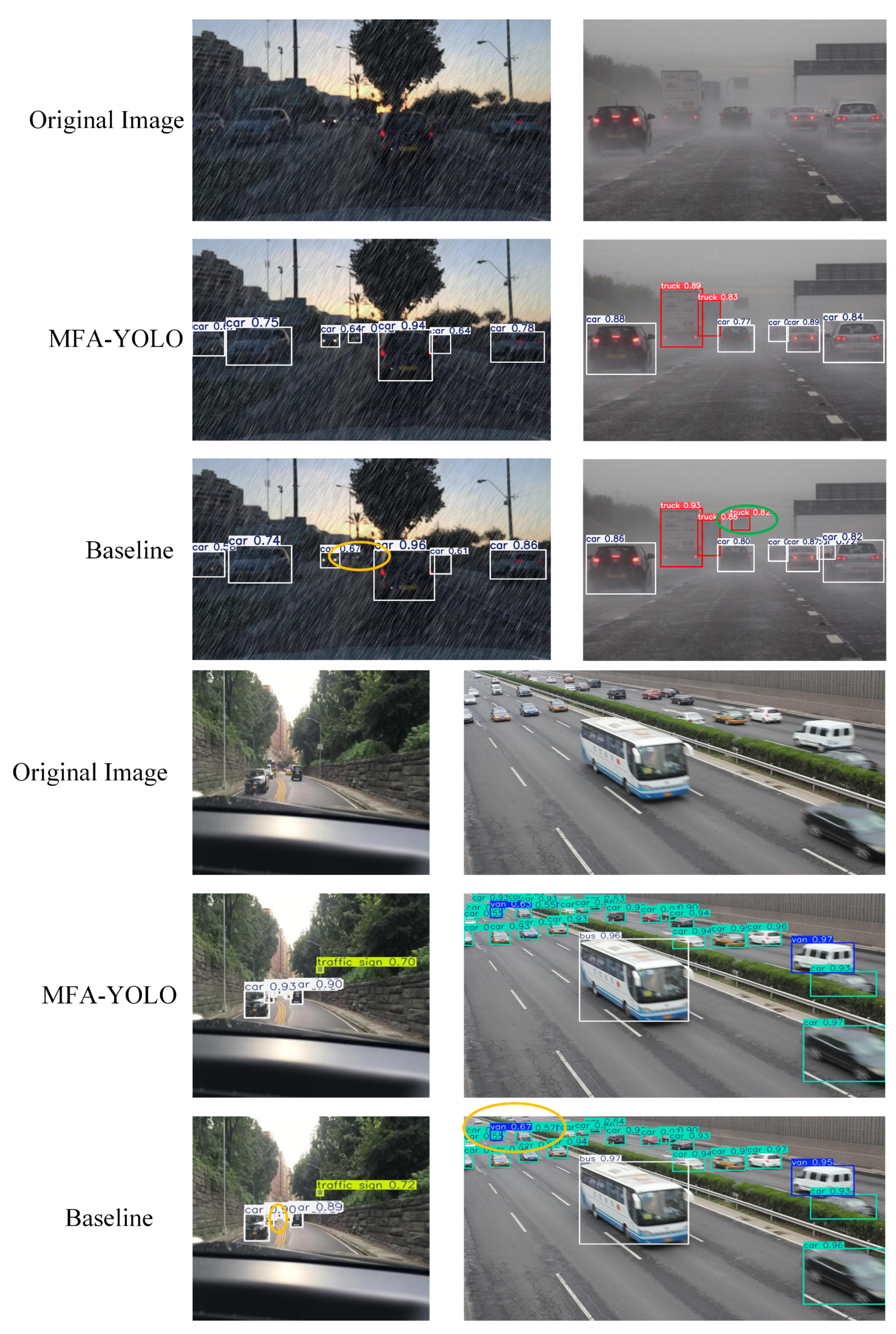
To visually illustrate the improvements of our algorithm over the original, we compare the detection performance of the baseline and MFA-YOLO in Figure 9. The top panel displays the original image, the middle panel shows the detection output of MFA-YOLO, and the bottom panel presents the detection results of the baseline model. Red circles highlight misdetected objects, while yellow circles indicate missed objects. As shown in the figure, MFA-YOLO demonstrates a significant enhancement in detection performance under complex road conditions and extreme weather compared to the baseline. The first two images originate from EWD dataset, the third image is sourced from GAD dataset, and the fourth image is derived from UA-DETRAC dataset. Comparing the detection results from the first image of the EWD dataset, it is evident that the baseline missed the smaller target vehicle, while MFA-YOLO successfully detected all vehicles. The second image, also from the EWD dataset, depicts a highway scene in heavy fog. In this case, the baseline incorrectly identified the highway sign as a truck, whereas MFA-YOLO did not make this error. The third image, from the GAD dataset, shows that the baseline missed smaller vehicles in the distance, a problem that MFA-YOLO avoided. Finally, the fourth image from the UA-DETRAC dataset clearly demonstrates that the baseline missed several smaller vehicles in the upper left corner, while MFA-YOLO detected all of them.

We analyzed the computational efficiency of each algorithm using the EWD dataset, evaluating and comparing latency, FPS, and other performance indicators. This analysis is crucial for discussing the practical application of our algorithm on edge devices. We compared computational efficiency using several metrics, including latency (in milliseconds, ms), FPS (frames per second), CPU memory usage (in MB), GPU memory usage (in MB), and FLOPS (in GigaFLOPS, or billion floating-point operations per second, ${10}^9$ FLOPS).

In addition, we have included a comparison with the YOLO-MobileNetV3 (YOLO-MN3) algorithm in the computational efficiency comparison table. YOLO-MN3 substitutes the backbone network of YOLOv11 with that of MobileNetV3, while the other components remain unchanged. MobileNetV3 is a lightweight CNN architecture designed specifically for mobile devices and embedded systems, aiming to reduce computational complexity while preserving high accuracy. This comparison with YOLO-MN3 serves to comprehensively evaluate the computational efficiency of our algorithm.

From the data presented in

Table 4. Comparison of computational efficiency of various algorithms.

Algorithm	Latency	FPS	CPU Memory	GPU Memory	FLOPS
MFA-YOLO	18.1	55.25	1408	1764	6.58
YOLOv11	18.7	53.48	1430	1799	6.44
YOLO-MN3	18.2	54.95	1400	1760	6.28
YOLOv10	20.8	48.08	1418	1792	8.40
YOLOv9	21.1	47.39	1453	1815	6.70
YOLOv8	22.4	44.64	1420	1789	6.94
YOLOv5	25.2	39.68	1470	1834	5.94
Faster R-CNN	39.2	25.51	1918	2456	8.32
SSD	28.3	35.34	1562	1978	6.58
RT-DETR	36.8	27.17	2203	2207	11.6

, we observe that the MFA-YOLO algorithm we proposed consistently exhibits lower latency. This indicates that MFA-YOLO achieves an excellent FPS, meaning it can process more images per second. Additionally, the CPU and GPU memory usage, as well as the FLOPS, are slightly lower than those of the baseline model. When considering the previous comparison of accuracy, recall rate, and mAP, it is evident that our algorithm offers better performance and computational efficiency, making it highly suitable for deployment on edge devices, which have specific requirements for both accuracy and latency. Furthermore, the Faster R-CNN algorithm exhibits relatively high overall latency due to its two-stage mechanism. The RT-DETR algorithm, on the other hand, has the highest FLOPS value, stemming from the complexity of the Transformer architecture, which consequently results in higher latency.

4.5. Identification Under Variable Fog Density

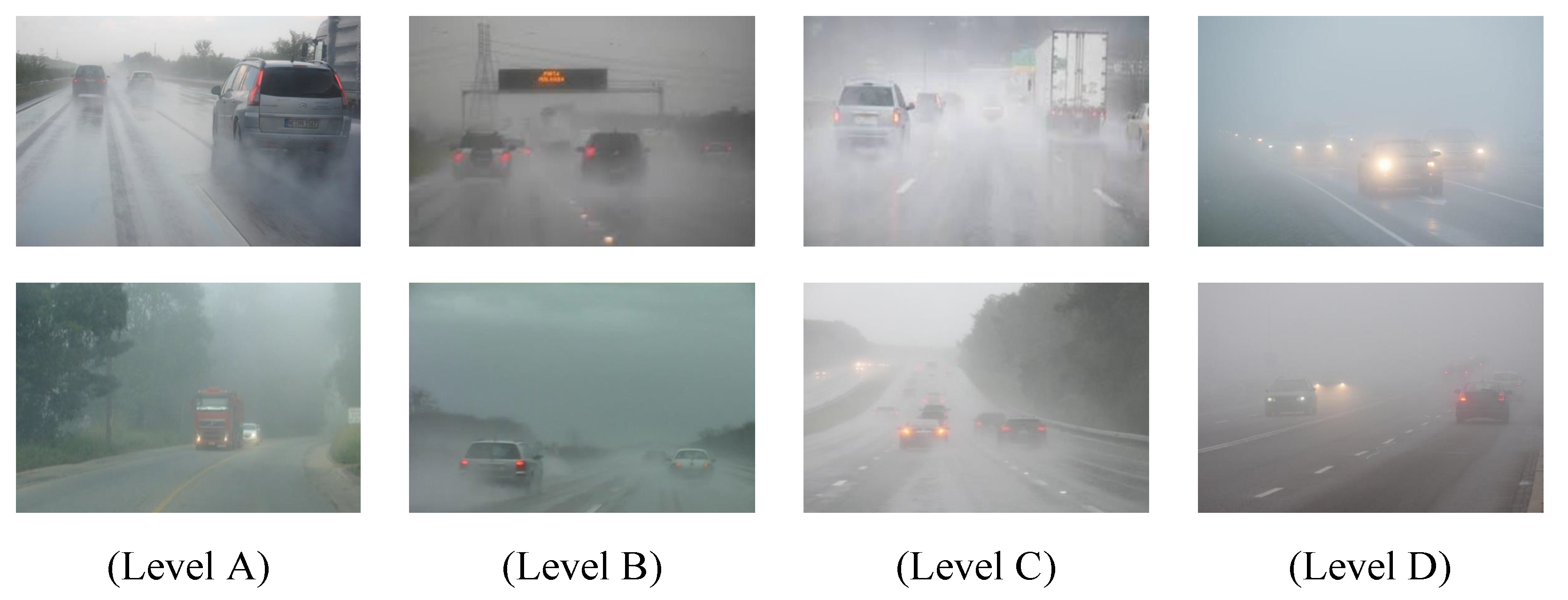
To assess the robustness and performance of the experimental algorithm under varying weather conditions, specifically with changing fog density, we categorized the foggy scenes in the dataset into four levels: Level A (light fog), Level B (moderate fog), Level C (heavy fog), and Level D (severe fog), as illustrated in Figure 10.

At Level A, the image brightness and contrast are high, and the details remain clear, with the fog being relatively light. At Level B, both brightness and contrast are moderate, and, while the image details are still discernible, they are slightly blurred, with noticeable fog present. At Level C, the image becomes noticeably blurred, with lower brightness and contrast, reflecting a more severe fog condition. Finally, at Level D, the image suffers from very low brightness and contrast, with details nearly invisible and the fog environment severely impeding visibility, making recognition almost impossible. We divided the fog-related portion of the dataset into four levels, trained each level separately, and created a comparison table of various algorithms under different fog conditions, as shown in

Table 5. Comparison of mAP values of different algorithms under different levels of fog.

Algorithm	Level A	Level B	Level C	Level D
MFA-YOLO	63.5	62.6	61.9	61.2
YOLOv11	58.3	57.9	56.1	54.2
YOLOv10	56.2	56.8	54.0	53.0
YOLOv9	54.5	54.4	52.8	51.8
YOLOv8	54.9	55.2	52.9	51.9
YOLOv5	53.2	51.6	51.6	51.5
Faster R-CNN	52.8	51.3	49.8	49.6
SSD	51.3	50.4	48.9	48.7
RT-DETR	56.8	56.6	55.5	54.5

. It is important to note that this comparison focuses solely on mAP.

As shown in Table 5, MFA-YOLO demonstrates better robustness and performs well across all four fog levels. Notably, from Level C to Level D, the performance of other algorithms significantly declines due to reduced visibility, while MFA-YOLO experiences only minimal performance degradation.

4.6. Ablation Experiment

To illustrate the effectiveness of various improvements, we also conducted ablation experiments using YOLOv11 as the baseline and plotted the experimental results in

Table 6. Comparison of ablation experiments on the EWD dataset.

Algorithm	Precision	Recall	mAP
YOLOv11 (Baseline)	65.3	54.7	56.1
YOLOv11 + WTConv	67.0	56.5	57.8
YOLOv11 + WTConv + SimSPPF+	68.2	57.0	59.1
YOLOv11 + WTConv + SimSPPF ++ HAFM	69.8	58.8	61.0
YOLOv11 + WTConv + SimSPPF ++ HAFM + BE-ATFL	71.5	61.2	62.7
MFA-YOLO (Ours)	72.2	62.5	63.9

.

From the data in Table 6, it is evident that the baseline model exhibits the poorest performance. By incorporating wavelet convolution, the model’s performance improves to some extent, with the mAP increasing by approximately $1.7\%$. When SimSPPF+ is applied, there is a slight further improvement, resulting in an additional mAP increase of about $1.3\%$. The inclusion of the HAFM module further enhances the mAP by $1.9\%$. With the implementation of BE-ATFL, the model achieves a notable improvement, with an mAP that is $1.7\%$ higher than the previous level. Finally, the final boost in performance comes with the last step, resulting in a total mAP of $63.9\%$, which represents a $7.8\%$ improvement over the baseline model. This clearly demonstrates the effectiveness of our enhancements under extreme weather conditions.

Additionally, to evaluate the impact of BE-ATFL on the algorithm, we conducted an ablation study comparing the proposed BE-ATFL with several commonly used focal loss functions, such as Generalized Focal Loss and Asymmetric Loss. The results are summarized in

Table 7. Ablation study on focal loss functions using the EWD dataset.

Algorithm	Precision	Recall	mAP
MFA-YOLO with Original Focal Loss	71.2	61.3	62.8
MFA-YOLO with Generalized Focal Loss	71.9	61.8	63.8
MFA-YOLO with Asymmetric Loss	71.4	62.3	63.5
MFA-YOLO with ATFL	71.9	62.2	63.6
MFA-YOLO with BE-ATFL (Ours)	72.2	62.5	63.9

.

Table 7 illustrates the impact of different focal losses on the performance of the MFA-YOLO algorithm. The ablation experiment reveals that the use of various improved focal losses enhances accuracy, recall, and mAP. Among them, the MFA-YOLO algorithm with the BE-ATFL focal loss outperforms the others across all metrics, demonstrating that BE-ATFL effectively boosts the model’s performance.

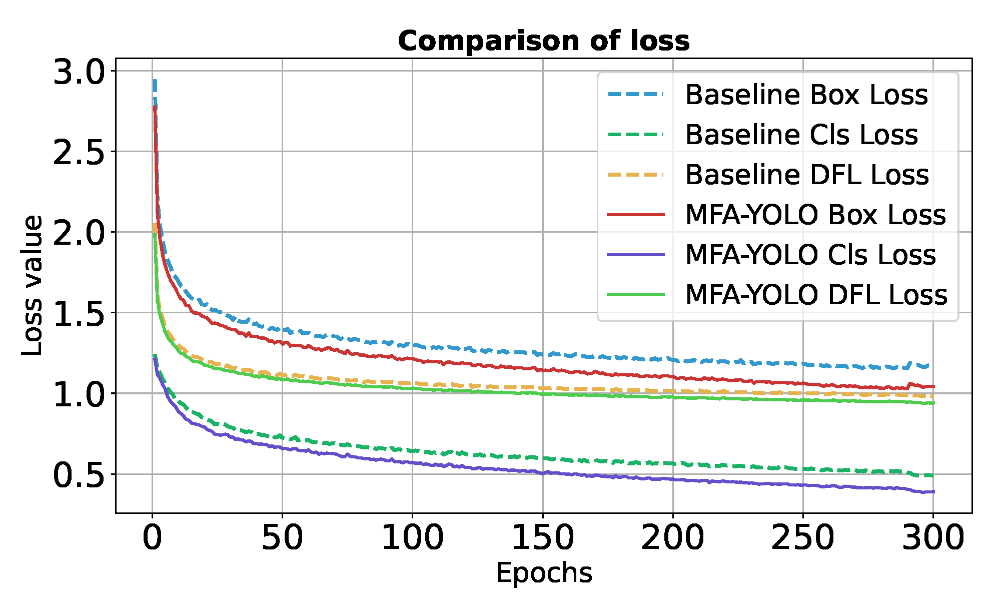
Figure 11 presents a comparison of the training loss curves between the baseline model and the improved MFA-YOLO model. As shown in the figure, MFA-YOLO demonstrates a clear trend of rapid convergence during the training process. In the first 50 training epochs, the loss value decreases almost exponentially, indicating that the algorithm quickly adapts to the training data distribution and learns a substantial amount of effective features and information. As the number of training epochs increases, the loss value gradually stabilizes. After 200 epochs, the loss value remains low, suggesting that the model is approaching its optimal solution. This rapid convergence highlights the efficiency of the MFA-YOLO model in the optimization process, enabling it to achieve better performance in less time. In contrast, the baseline model converges more slowly. While the loss value decreases in the early stages, the reduction is not as significant as that of MFA-YOLO. Even after 300 epochs, the loss value remains relatively high, indicating that its optimization process is slower and does not achieve the same results as MFA-YOLO within the same number of training rounds. The loss curve clearly demonstrates that MFA-YOLO achieves lower loss values across all loss functions, indicating better optimization and convergence during training. Furthermore, under the current experimental settings, MFA-YOLO requires 25.8 h to train, while the baseline model takes 27.4 h.

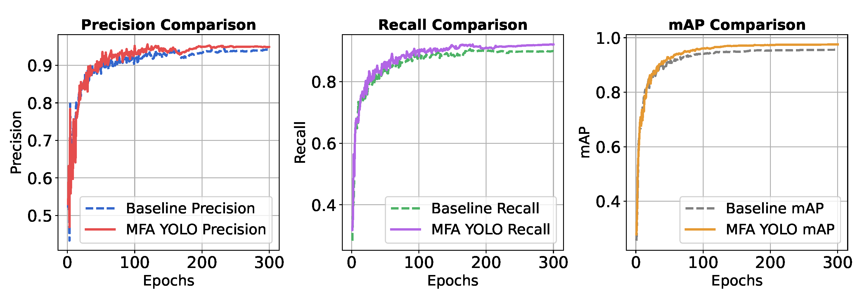
Figure 12 illustrates the curve comparison for three metrics—precision (P), recall (R), and mAP—between the baseline model and MFA-YOLO. In the figures, solid lines represent MFA-YOLO, while dashed lines represent the baseline model. It can be observed that MFA-YOLO consistently outperforms the baseline model in all three metrics, reflecting its superior detection performance and accuracy.

4.7. Generalization to Other Domains

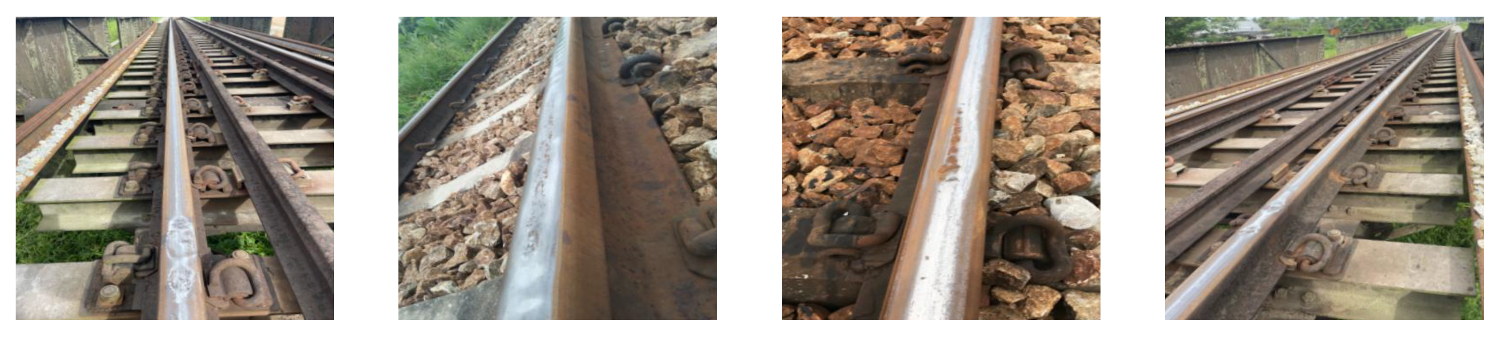
Previous experiments have demonstrated that our algorithm performs well in autonomous driving under various conditions. Next, we explore its potential applications in other fields. One such area that piqued our interest is rail defect detection. Rail defect detection involves using various technical methods to inspect railway rails for potential defects. As rails are a critical component of the railway transportation system, their condition is directly linked to train safety. The primary goal of defect detection is to identify issues such as cracks, wear, fractures, deformations, and other surface problems that could lead to accidents.

For the experiments, we utilize the CSRDR rail defect detection dataset, which consists of 4020 images with four labels: Corrugation, Spalling, Squat, and Wheel Burn. Figure 13 shows some simple examples of the CSRDR dataset. In this subsection, we maintain the same experimental parameters as in the previous settings.

As in the previous experiments, we compared the performance of different algorithms on this dataset, and the results are presented in

Table 8. Comparison of algorithms on rail defect detection tasks.

Algorithm	Precision	Recall	mAP
MFA-YOLO (Ours)	70.6	60.8	61.7
YOLOv11	62.4	53.2	54.2
YOLOv10	59.7	50.2	51.9
YOLOv9	59.2	49.9	49.8
YOLOv8	61.3	50.7	50.2
YOLOv5	57.3	49.6	48.6
Faster R-CNN	54.9	48.1	47.2
SSD	52.8	47.2	45.8
RT-DETR	60.1	50.5	51.7

.

As shown in Table 8, MFA-YOLO also demonstrated strong performance on this dataset, outperforming other algorithms in terms of precision, recall, and mAP. This highlights the robustness and generalization capabilities of MFA-YOLO. Although originally designed for autonomous driving in extreme weather conditions, the algorithm can seamlessly adapt to tasks in various domains and perform exceptionally well across different applications.

5. Conclusions

To address the challenges of detecting and recognizing small and obscured vehicles in the distance under extreme weather conditions, this paper proposes an improved detection algorithm, MFA-YOLO, based on YOLO v11. The proposed C3k2-WT module, leveraging wavelet transform, effectively extracts features from different frequency components and captures information across multiple fields of view. Additionally, spatial pooling is utilized to enhance the traditional SPPF module, resulting in the SimSPPF+ module, which improves the recognition of elongated objects. The SPM module is also applied before the detection head to optimize the extraction and recognition of feature information. Furthermore, we introduce the C2PSA-HAFM module to hierarchically fuse global attention with local features, incorporating the GELU activation function to complement the attention mechanism. From the perspective of loss functions, we propose the BE-ATFL classification loss function to enhance the detection and recognition of small edge targets effectively. Finally, the effectiveness and superiority of the proposed algorithm were validated through experiments on the EWD, GAD, and UA-DETRAC datasets, with comparisons to other advanced algorithms demonstrating its ability to address the challenges outlined at the beginning of this study. Future work will focus on further optimizing the model and extending its application to more realistic scenarios, addressing increasingly complex tasks. For instance, in addition to traditional data augmentation techniques, we plan to leverage Generative Adversarial Networks (GANs) for data augmentation and explore additional real-world scenarios, such as adversarial conditions, intensity fluctuations, and sensor noise.