


Optimizing Multi-View CNN for CAD Mechanical Model Classification: An Evaluation of Pruning and Quantization Techniques


Abstract
1. Introduction
- We analyze the effects of varying pruning ratios on the MVCNN model’s performance, evaluating trade-offs between classification accuracy, execution time, and memory demanded by the model. Furthermore, we examine the impact of applying quantization to the original MVCNN model, assessing its effect on the performance metrics stated above.
- In addition, we analyze the simultaneous application of both pruning and quantization and its impact on those performance indicators.
2. Background
3. Materials and Methods

| Repository | Number of Models | Number of Classes | Normalized Entropy |
|---|---|---|---|
| Mechanical Components Benchmark (MCB) [19] | 58,696 | 68 | 0.814 |
| CADNET [24] | 3317 | 43 | 0.984 |
| Engineering Shape Benchmark (ESB) [25] | 801 | 45 | 0.937 |
| MCB-B [19] | 18,038 | 25 | 0.848 |
3.1. Data Preparation
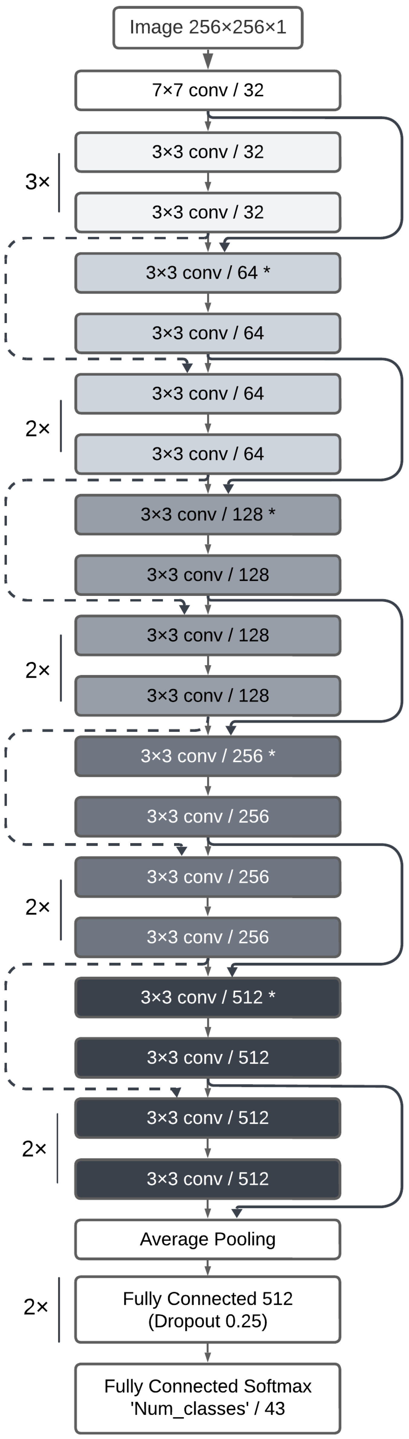
3.2. Model Architecture
3.3. Experimental Setup
3.4. Optimization Techniques
4. Results
5. Conclusions
Author Contributions
Funding
Data Availability Statement
Conflicts of Interest
Abbreviations
| CAD | computer-aided design |
| ML | machine learning |
| DL | deep learning |
| CNN | convolutional neural network |
| PCNN | point cloud convolutional neural network |
| MVCNN | multi-view convolutional neural network |
| STL | stereolithography |
| MCB | Mechanical Component Benchmark |
| ESB | Engineering Shape Benchmark |
References
- Mandelli, L.; Berretti, S. CAD 3D Model classification by graph neural networks: A new approach based on STEP format. arXiv 2022, arXiv:2210.16815. [Google Scholar] [CrossRef]
- Bonino, B.; Giannini, F.; Monti, M.; Raffaeli, R. Shape and context-based recognition of standard mechanical parts in CAD models. Comput.-Aided Des. 2023, 155, 103438. [Google Scholar] [CrossRef]
- Fang, H.C.; Ong, S.K.; Nee, A.Y.C. Product remanufacturability assessment based on design information. Procedia CIRP 2014, 15, 195–200. [Google Scholar] [CrossRef]
- Iancu, C.; Iancu, D.; Stăncioiu, A. From CAD model to 3D print via “STL” file format. Fiability Durability/Fiabilitate Durabilitate 2010, 1, 73–80. [Google Scholar]
- Kim, H.; Yeo, C.; Lee, I.D.; Mun, D. Deep-learning-based retrieval of piping component catalogs for plant 3D CAD model reconstruction. Comput. Ind. 2020, 123, 103320. [Google Scholar] [CrossRef]
- Adesso, M.F.; Hegewald, R.; Wolpert, N.; Schömer, E.; Maier, B.; Epple, B.A. Automatic classification and disassembly of fasteners in industrial 3D CAD-Scenarios. In Proceedings of the 2022 International Conference on Robotics and Automation (ICRA), Philadelphia, PA, USA, 23–27 May 2022; pp. 9874–9880. [Google Scholar] [CrossRef]
- Ip, C.Y.; Regli, W.C. A 3D object classifier for discriminating manufacturing processes. Comput. Graph. 2006, 30, 903–916. [Google Scholar] [CrossRef]
- Hernavs, J.; Ficko, M.; Klančnik, L.; Rudolf, R.; Klančnik, S. Deep learning in industry 4.0—Brief overview. J. Prod. Eng. 2018, 21, 1–5. [Google Scholar] [CrossRef]
- Heidari, N.; Iosifidis, A. Geometric deep learning for computer-aided design: A survey. arXiv 2024, arXiv:2402.17695. [Google Scholar] [CrossRef]
- Wang, C.; Cheng, M.; Sohel, F.; Bennamoun, M.; Li, J. NormalNet: A voxel-based CNN for 3D object classification and retrieval. Neurocomputing 2019, 323, 139–147. [Google Scholar] [CrossRef]
- Atzmon, M.; Maron, H.; Lipman, Y. Point convolutional neural networks by extension operators. arXiv 2018, arXiv:1803.10091. [Google Scholar] [CrossRef]
- Qi, S.; Ning, X.; Yang, G.; Zhang, L.; Long, P.; Cai, W.; Li, W. Review of multi-view 3D object recognition methods based on deep learning. Displays 2021, 69, 102053. [Google Scholar] [CrossRef]
- Gezawa, A.S.; Zhang, Y.; Wang, Q.; Lei, Y. A review on deep learning approaches for 3D data representations in retrieval and classifications. IEEE Access 2020, 8, 57566–57593. [Google Scholar] [CrossRef]
- Qi, C.R.; Su, H.; Nießner, M.; Dai, A.; Yan, M.; Guibas, L.J. Volumetric and multi-view CNNs for object classification on 3d data. In Proceedings of the IEEE Conference on Computer Vision and Pattern Recognition, Las Vegas, NV, USA, 26 June–1 July 2016; pp. 5648–5656. [Google Scholar] [CrossRef]
- Kanezaki, A.; Matsushita, Y.; Nishida, Y. Rotationnet: Joint object categorization and pose estimation using multiviews from unsupervised viewpoints. In Proceedings of the IEEE Conference on Computer Vision and Pattern Recognition, Salt Lake City, UT, USA, 18–23 June 2018; pp. 5010–5019. [Google Scholar] [CrossRef]
- Wu, J.; Leng, C.; Wang, Y.; Hu, Q.; Cheng, J. Quantized convolutional neural networks for mobile devices. In Proceedings of the IEEE Conference on Computer Vision and Pattern Recognition, Las Vegas, NV, USA, 27–30 June 2016; pp. 4820–4828. [Google Scholar] [CrossRef]
- Li, G.; Wang, J.; Shen, H.W.; Chen, K.; Shan, G.; Lu, Z. CNNpruner: Pruning convolutional neural networks with visual analytics. IEEE Trans. Vis. Comput. Graph. 2020, 27, 1364–1373. [Google Scholar] [CrossRef]
- Wei, X.; Yu, R.; Sun, J. View-GCN: View-based graph convolutional network for 3D shape analysis. In Proceedings of the IEEE/CVF Conference on Computer Vision and Pattern Recognition, Seattle, WA, USA, 13–19 June 2020; pp. 1850–1859. [Google Scholar] [CrossRef]
- Kim, S.; Chi, H.G.; Hu, X.; Huang, Q.; Ramani, K. A large-scale annotated mechanical components benchmark for classification and retrieval tasks with deep neural networks. In Computer Vision—ECCV 2020, Proceedings of the 16th European Conference, Glasgow, UK, 23–28 August 2020; Springer: Cham, Switzerland, 2020; Part XVIII; pp. 175–191. [Google Scholar] [CrossRef]
- Li, S.; Corney, J. Multi-view expressive graph neural networks for 3D CAD model classification. Comput. Ind. 2023, 151, 103993. [Google Scholar] [CrossRef]
- Kuzmin, A.; Nagel, M.; Van Baalen, M.; Behboodi, A.; Blankevoort, T. Pruning vs quantization: Which is better? In Advances in Neural Information Processing Systems, Proceedings of the 37th International Conference on Neural Information Processing Systems, New Orleans, LA, USA, 10–16 December 2023; Curran Associates Inc.: Red Hook, NY, USA, 2023; Volume 36, pp. 62414–62427. [Google Scholar]
- Tian, Q.; Arbel, T.; Clark, J.J. Grow-push-prune: Aligning deep discriminants for effective structural network compression. Comput. Vis. Image Underst. 2023, 231, 103682. [Google Scholar] [CrossRef]
- Lima, V.S.; Ferreira, F.A.; Madeiro, F.; Lima, J.B. Light field image encryption based on steerable cosine number transform. Signal Process. 2023, 202, 108781. [Google Scholar] [CrossRef]
- Manda, B.; Bhaskare, P.; Muthuganapathy, R. A convolutional neural network approach to the classification of engineering models. IEEE Access 2021, 9, 22711–22723. [Google Scholar] [CrossRef]
- Iyer, N.; Jayanti, S.; Ramani, K. An engineering shape benchmark for 3D models. In International Design Engineering Technical Conferences and Computers and Information in Engineering Conference, Long Beach, CA, USA, 24–28 September 2005; ASME: New York, NY, USA, 2005; Volume 47403, pp. 501–509. [Google Scholar] [CrossRef]
- Francazi, E.; Baity-Jesi, M.; Lucchi, A. A theoretical analysis of the learning dynamics under class imbalance. In Proceedings of the 40th International Conference on Machine Learning, Honolulu, HI, USA, 23–29 July 2023; pp. 10285–10322. Available online: https://dl.acm.org/doi/proceedings/10.5555/3618408 (accessed on 12 February 2025).
- Chen, W.; Yang, K.; Yu, Z.; Shi, Y.; Chen, C.L. A survey on imbalanced learning: Latest research, applications and future directions. Artif. Intell. Rev. 2024, 57, 137. [Google Scholar] [CrossRef]
- Johnson, J.M.; Khoshgoftaar, T.M. Survey on deep learning with class imbalance. J. Big Data 2019, 6, 27. [Google Scholar] [CrossRef]
- Santos, C.F.G.D.; Papa, J.P. Avoiding overfitting: A survey on regularization methods for convolutional neural networks. ACM Comput. Surv. (CSUR) 2022, 54, 213. [Google Scholar] [CrossRef]
- Kwasniewska, A.; Szankin, M.; Ozga, M.; Wolfe, J.; Das, A.; Zajac, A.; Ruminski, J.; Rad, P. Deep learning optimization for edge devices: Analysis of training quantization parameters. In Proceedings of the IECON 2019—45th Annual Conference of the IEEE Industrial Electronics Society, Lisbon, Portugal, 14–17 October 2019; Volume 1, pp. 96–101. [Google Scholar] [CrossRef]
- Jacob, B.; Kligys, S.; Chen, B.; Zhu, M.; Tang, M.; Howard, A.; Adam, H.; Kalenichenko, D. Quantization and training of neural networks for efficient integer-arithmetic-only inference. In Proceedings of the IEEE Conference on Computer Vision and Pattern Recognition, Salt Lake City, UT, USA, 18–23 June 2018; pp. 2704–2713. [Google Scholar] [CrossRef]
- Liang, T.; Glossner, J.; Wang, L.; Shi, S.; Zhang, X. Pruning and quantization for deep neural network acceleration: A survey. Neurocomputing 2021, 461, 370–403. [Google Scholar] [CrossRef]
- Chen, S.; Wang, W.; Pan, S.J. Deep neural network quantization via layer-wise optimization using limited training data. In Proceedings of the AAAI Conference on Artificial Intelligence, Honolulu, HI, USA, 27 January–1 February 2019; Volume 33, pp. 3329–3336. [Google Scholar] [CrossRef]
- Li, H.; Kadav, A.; Durdanovic, I.; Samet, H.; Graf, H.P. Pruning filters for efficient convnets. arXiv 2016, arXiv:1608.08710. [Google Scholar] [CrossRef]
- Banner, R.; Hubara, I.; Hoffer, E.; Soudry, D. Scalable methods for 8-bit training of neural networks. In Advances in Neural Information Processing Systems, Proceedings of the 32nd International Conference on Neural Information Processing Systems, Montreal, QC, Canada, 3–8 December 2018; Curran Associates Inc.: Red Hook, NY, USA, 2018; Volume 31. [Google Scholar]
- Chen, C. Hardware-Software Co-Exploration and Optimization for Next-Generation Learning Machines. Ph.D. Thesis, Nanyang Technological University, Singapore, 2024. Available online: https://dr.ntu.edu.sg/bitstream/10356/178423/2/PhD_Thesis_ChenChunyun-Final.pdf (accessed on 18 December 2024).
- Wei, L.; Ma, Z.; Yang, C.; Yao, Q. Advances in the neural network quantization: A comprehensive review. Appl. Sci. 2024, 14, 7445. [Google Scholar] [CrossRef]

| Category Name | Number of 3D Objects | Category Name | Number of 3D Objects |
|---|---|---|---|
| 90_degree_elbows | 100 | Gear_like_Parts | 97 |
| BackDoors | 57 | Handles | 119 |
| Bearing_Blocks | 50 | Intersecting_Pipes | 50 |
| Bearing_Like_Parts | 50 | L_Blocks | 107 |
| Bolt_Like_Parts | 111 | Long_Machine_Elements | 77 |
| Bracket_like_Parts | 27 | Long_Pins | 104 |
| Clips | 54 | Machined_Blocks | 59 |
| Contact_Switches | 60 | Machined_Plates | 99 |
| Container_Like_Parts | 60 | Motor_Bodies | 58 |
| Contoured_Surfaces | 55 | Non-90_degree_elbows | 108 |
| Curved_Housings | 51 | Nuts | 125 |
| Cylindrical_Parts | 94 | Oil_Pans | 58 |
| Discs | 163 | Posts | 109 |
| Flange_Like_Parts | 109 | Prismatic_Stock | 86 |
| Pulley_Like_Parts | 61 | Rectangular_Housings | 70 |
| Rocker_Arms | 60 | Round_Change_At_End | 51 |
| Screws | 111 | Simple_Pipes | 66 |
| Slender_Links | 60 | Slender_Thin_Plates | 62 |
| Small_Machined_Blocks | 62 | Spoked_Wheels | 57 |
| Springs | 55 | Thick_Plates | 82 |
| Thin_Plates | 83 | T-shaped_parts | 65 |
| U-shaped_parts | 75 | ||
| Number of 3D Objects | 3317 |
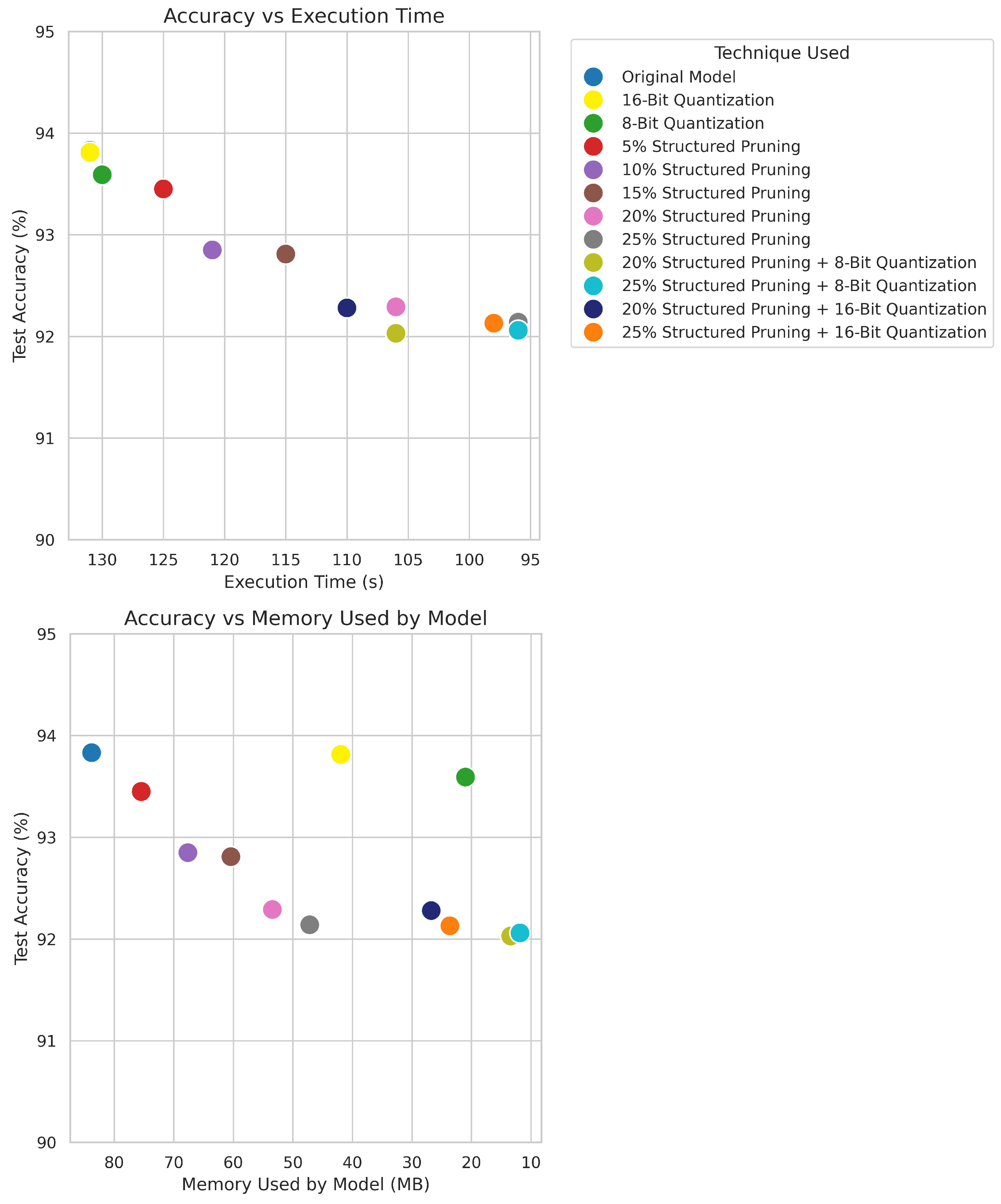
| Technique Used | Test Accuracy (%) | Execution Time (s) | Memory Occupied by the Model (MB) |
|---|---|---|---|
| Original Model | 93.83 | 133 | 83.78 |
| 16-Bit Quantization | 93.81 | 133 | 41.94 |
| 8-Bit Quantization | 93.59 | 132 | 21.01 |
| 4-Bit Quantization | 23.11 | 134 | 10.55 |
| 5% Structured Pruning | 93.45 | 127 | 75.45 |
| 10% Structured Pruning | 92.85 | 123 | 67.62 |
| 15% Structured Pruning | 92.81 | 117 | 60.40 |
| 20% Structured Pruning | 92.29 | 110 | 53.43 |
| 25% Structured Pruning | 92.14 | 97 | 47.16 |
| 5% Structured Pruning + 16-Bit Quantization | 93.45 | 127 | 37.77 |
| 10% Structured Pruning + 16-Bit Quantization | 92.85 | 123 | 33.86 |
| 15% Structured Pruning + 16-Bit Quantization | 92.80 | 117 | 30.25 |
| 20% Structured Pruning + 16-Bit Quantization | 92.28 | 110 | 26.76 |
| 25% Structured Pruning + 16-Bit Quantization | 92.13 | 98 | 23.63 |
| 5% Structured Pruning + 8-Bit Quantization | 93.35 | 128 | 18.93 |
| 10% Structured Pruning + 8-Bit Quantization | 92.80 | 124 | 16.97 |
| 15% Structured Pruning + 8-Bit Quantization | 92.69 | 118 | 15.17 |
| 20% Structured Pruning + 8-Bit Quantization | 92.03 | 110 | 13.42 |
| 25% Structured Pruning + 8-Bit Quantization | 92.06 | 99 | 11.86 |
Disclaimer/Publisher’s Note: The statements, opinions and data contained in all publications are solely those of the individual author(s) and contributor(s) and not of MDPI and/or the editor(s). MDPI and/or the editor(s) disclaim responsibility for any injury to people or property resulting from any ideas, methods, instructions or products referred to in the content. |
© 2025 by the authors. Licensee MDPI, Basel, Switzerland. This article is an open access article distributed under the terms and conditions of the Creative Commons Attribution (CC BY) license (https://creativecommons.org/licenses/by/4.0/).
Share and Cite
Pinto, V.; Severo, V.; Madeiro, F. Optimizing Multi-View CNN for CAD Mechanical Model Classification: An Evaluation of Pruning and Quantization Techniques. Electronics 2025, 14, 1013. https://doi.org/10.3390/electronics14051013
Pinto V, Severo V, Madeiro F. Optimizing Multi-View CNN for CAD Mechanical Model Classification: An Evaluation of Pruning and Quantization Techniques. Electronics. 2025; 14(5):1013. https://doi.org/10.3390/electronics14051013
Chicago/Turabian StylePinto, Victor, Verusca Severo, and Francisco Madeiro. 2025. "Optimizing Multi-View CNN for CAD Mechanical Model Classification: An Evaluation of Pruning and Quantization Techniques" Electronics 14, no. 5: 1013. https://doi.org/10.3390/electronics14051013
APA StylePinto, V., Severo, V., & Madeiro, F. (2025). Optimizing Multi-View CNN for CAD Mechanical Model Classification: An Evaluation of Pruning and Quantization Techniques. Electronics, 14(5), 1013. https://doi.org/10.3390/electronics14051013