Artificial Intelligence-Based Fault Diagnosis for Steam Traps Using Statistical Time Series Features and a Transformer Encoder-Decoder Model

Abstract

Steam traps are essential for industrial systems, ensuring steam quality and energy efficiency by removing condensate and preventing steam leakage. However, their failure results in energy loss, operational disruptions, and increased greenhouse gas emissions. This paper proposes a novel predictive maintenance system for steam traps that integrates statistical time series features and transformer encoder–decoder models for fault diagnosis and visualization. The proposed system combines IoT sensor data, operational parameters, open data (e.g., weather information and public holiday calendars), machine learning, and two-dimensional diagnostic projection to improve reliability and interpretability. Experiments were conducted in two industrial plants: an aluminum processing plant and a food manufacturing plant, and the system achieved superior defect detection accuracy and diagnostic reliability compared to existing methods. The transformer-based model outperformed traditional methods, including random forest, gradient boosting, and variational autoencoder, in classification and clustering. The system also demonstrated an average 6.92% reduction in thermal energy across both sites, highlighting its potential to improve energy efficiency and reduce carbon emissions. This research highlights the transformative impact of AI-based predictive maintenance technologies in industrial operations and provides a framework for sustainable manufacturing practices.

1. Introduction

1.1. Challenges in Steam Trap Maintenance

Steam traps play a crucial role in industrial steam systems by removing condensate and preventing steam leakage. Their effective management enhances energy efficiency and ensures operational reliability. However, failures in steam traps contribute to significant energy losses, production disruptions, and increased greenhouse gas emissions. Traditional maintenance practices, which rely on periodic manual inspections and reactive failure responses, suffer from inherent drawbacks:

• Manual inspections are time-consuming, labor-intensive, and prone to human error.
• Failures often go undetected for extended periods, leading to excessive energy waste.
• Unexpected failures result in production downtime and increased maintenance costs.

Although predictive maintenance technologies have improved real-time condition monitoring and automated fault diagnosis, practical challenges persist. These include sensor standardization issues, accessibility constraints, and maintenance delays caused by insulation barriers.

First, the lack of standardization among manufacturers complicates maintenance procedures. Each manufacturer employs different diagnostic methods and design specifications, making it difficult to establish a unified maintenance protocol [1]. Engineers must adapt to various diagnostic techniques, increasing training time and operational complexity.

Second, limited accessibility hinders routine inspections and emergency repairs. Many steam traps are installed in hard-to-reach areas, such as ceilings, underground spaces, or within dense piping networks. These locations make manual inspections challenging, delaying fault detection and increasing maintenance costs.

Third, insulation barriers add complexity to maintenance procedures. Most steam traps are covered with insulation materials to maintain steam quality and energy efficiency. However, these coverings must be removed for visual inspections, adding extra labor and downtime to the maintenance process [2].

These challenges underscore the limitations of traditional steam trap maintenance and highlight the necessity for more efficient, standardized, and automated solutions.

1.2. AI-Based Predictive Maintenance for Steam Trap Monitoring

To overcome the inefficiencies of traditional steam trap maintenance, including time-consuming manual inspections, undetected failures, limited accessibility, and the lack of standardized diagnostic protocols, this paper proposes a novel AI-based diagnostic system that integrates statistical time-series features with a Transformer encoder–decoder model. The proposed approach enhances fault detection accuracy and improves diagnostic reliability by leveraging advanced feature extraction and deep learning techniques.

Furthermore, this study introduces a comparative evaluation of various visualization methods to improve the interpretability of diagnostic results, enabling engineers to make more informed maintenance decisions.

The effectiveness of the proposed system is validated through real-world experiments in two industrial environments: an aluminum processing plant and a food manufacturing plant. The results demonstrate that the system achieves significant energy savings and enhances predictive maintenance capabilities. These contributions highlight the transformative potential of AI-driven predictive maintenance systems in optimizing industrial steam trap management, reducing energy waste, and promoting sustainable manufacturing practices [2].

1.3. Advancements in AI-Based Predictive Maintenance

Predictive maintenance, driven by AI methodologies, has significantly enhanced operational efficiency and minimized downtime. Recent advancements have focused on key areas such as sensor fusion, anomaly detection, and deep learning techniques.

Sensor Fusion: Integrating data from multiple sensors provides a comprehensive view of equipment health, leading to more accurate fault detection. Recent developments in AI-based predictive maintenance have focused on key components, trustworthiness, and future trends [3].

Anomaly Detection: Advanced AI algorithms have improved the identification of deviations from normal operational patterns, enabling early detection of potential failures. Recent studies have demonstrated the effectiveness of machine learning techniques in predictive maintenance, such as the use of deep learning models for anomaly detection in smart manufacturing [4], and the application of pattern mining-based algorithms to identify early signs of machinery malfunctioning [5].

Deep Learning Applications: Deep learning techniques have been extensively utilized in predictive maintenance to enhance fault detection and diagnosis. For instance, a study introduced a hybrid deep learning framework combining Convolutional Neural Networks (CNNs) and Recurrent Neural Networks (RNNs) to improve fault prediction accuracy in rotating machinery, thereby enhancing operational efficiency and reliability [6].

These advancements collectively contribute to more reliable and efficient maintenance strategies, leveraging AI to predict and prevent equipment failures proactively.

Recent studies have integrated AI-driven diagnostic frameworks for predictive maintenance in complex industrial settings, such as sensor fusion models for anomaly detection in industrial equipment [3].

These approaches highlight the growing need for advanced fault diagnosis techniques, particularly in energy optimization for industrial applications. The proposed Transformer-based diagnostic model builds on this foundation, integrating statistical time-series analysis with deep learning-based clustering for improved reliability and fault detection.

2. Related Works

Steam trap management is an important part of maintaining the energy efficiency and safety of industrial facilities. Existing steam trap management has mainly relied on regular inspections and passive failure response, but these methods make it difficult to implement preventive measures before a failure occurs. Because of these problems, recent research has focused on predictive maintenance technologies that can improve the performance of Steam Traps and prevent failures in advance.

2.1. Existing Steam Trap Management Methods

The management of steam traps presents a significant challenge in industrial environments, as incorrect maintenance leads to substantial energy loss and inefficiency [7]. Traditionally, steam trap inspections rely on manual monitoring, which suffers from accessibility issues due to installation locations, inconsistent monitoring cycles, and difficulty integrating real-time data. Significant research efforts have focused on using sensor-based monitoring systems to enhance predictive maintenance [2]. However, real-world applications face two main challenges:

• Heterogeneous sensor data collected from different manufacturers lacks standardization, making integration difficult [8].
• Environmental factors such as insulation layers and varying steam pressure complicate direct fault detection, requiring advanced methods such as infrared thermal imaging-based diagnostics [9].

These challenges necessitate advanced data processing techniques beyond traditional statistical methods.

The development of wireless smart sensors powered by thermoelectric generators has been reported to establish an online monitoring environment for steam traps [10]. This system diagnosed faults by analyzing whether the measured inlet and outlet temperatures of the steam trap fell within ranges corresponding to normal operation, blockage, or leakage, leading to improved steam energy efficiency. However, continuous operation posed challenges due to high energy consumption when the communication cycle was short.

A big data-driven prioritization model for steam trap maintenance has also been introduced, utilizing historical maintenance data to calculate failure probabilities and prioritize maintenance tasks through Failure Modes and Effects Analysis (FMEA) [2]. This systematic approach identified potential failure modes, assessed their impact, and prioritized corrective actions, resulting in high prediction accuracy and a significant reduction in the number of unnecessary inspections. Nevertheless, the model faced limitations due to its heavy reliance on initial data quality and the need for parameter weight adjustments.

2.2. Advancement of Predictive Maintenance Technology

Previous research has demonstrated the effectiveness of predictive maintenance in industrial applications. For instance, studies have applied Support Vector Machines (SVMs) for early fault detection in industrial pipelines [11] and leveraged deep learning techniques for anomaly detection in steam-based systems [12]. However, transferring these methods to steam trap diagnostics presents three challenges:

While predictive maintenance techniques have shown promise, applying them to steam trap diagnostics introduces three key challenges:

• Traditional models, such as PCA and t-SNE, provide dimensionality reduction but may fail to preserve both local and global structures in high-dimensional data, leading to suboptimal representation [13].
• Supervised learning models require extensive labeled datasets, which are not always available due to the cost of manual annotations. This limitation has been highlighted in studies addressing data collection and quality challenges in deep learning [14].
• Transformer-based models have demonstrated superior feature extraction capabilities for time-series data [15], but their application to steam trap diagnostics remains unexplored.

This paper integrates time-series statistical features with a Transformer encoder–decoder model for fault detection and visualization to address these gaps. The proposed approach combines sensor fusion with deep learning, enabling enhanced diagnostic accuracy and interpretability.

One notable development in predictive maintenance is the adoption of distributed AI systems. These systems allow for seamless integration and analysis of data across manufacturing plants, reducing maintenance costs and increasing fault detection accuracy through feature selection and real-time monitoring. For instance, research has shown that distributed frameworks effectively enable plant-wide monitoring and facilitate dynamic fault diagnostics across various industrial environments [16,17].

In addition, deep learning models have proven to be instrumental in predictive maintenance by processing high-dimensional and complex sensor data to identify patterns and predict equipment failures. Recent studies highlighted the ability of deep learning algorithms to analyze large datasets, prioritize maintenance tasks, and enhance fault detection rates. This underscores the role of machine learning as a critical enabler of predictive maintenance, allowing for proactive decision-making and resource optimization [18].

IoT and cloud-based solutions also play a pivotal role in modern predictive maintenance systems. These technologies provide scalable platforms for real-time data collection and analysis, enabling industries to implement efficient monitoring frameworks across geographically distributed facilities. By leveraging IoT-enabled sensors and cloud computing, predictive maintenance systems can significantly reduce equipment failures while improving operational efficiency, as demonstrated in multiple industrial case studies [19].

Distributed systems for predictive maintenance further integrate these technologies to create unified monitoring platforms capable of handling real-time data from multiple locations. This comprehensive approach not only enhances equipment health monitoring but also utilizes advanced machine learning techniques for fault diagnosis and feature extraction. Such frameworks exemplify the synergy between AI and IoT technologies, ensuring that the relevant maintenance strategies are data-driven and precise [16,17].

The advancements in predictive maintenance have profoundly impacted industrial sectors, including manufacturing and process industries, by increasing reliability, reducing downtime, and optimizing operational performance. As the integration of AI and IoT technologies continues to evolve, future research may focus on refining predictive models, improving computational efficiency, and addressing challenges related to data quality and system interoperability.

Dimensionality Reduction and Visualization Techniques

Conventional techniques like Principal Component Analysis (PCA), t-Distributed Stochastic Neighbor Embedding (t-SNE), and Variational Autoencoder (VAE) have been widely used in data visualization and representation tasks. PCA focuses on variance maximization to reduce dimensionality but may overlook subtle diagnostic patterns relevant to fault detection. t-SNE optimizes local similarity, effectively capturing local structures in high-dimensional data; however, it struggles to preserve global relationships, limiting its interpretability in comprehensive diagnostic scenarios. VAE encodes data into latent spaces that can capture complex patterns but often lacks direct interpretability for specific diagnostic tasks.

2.3. Transformer Encoder–Decoder Model in Fault Diagnosis

The Transformer encoder–decoder model provides significant advantages for fault detection and diagnosis in high-dimensional time-series data. Unlike recurrent models, which process sequences sequentially, the Transformer employs a self-attention mechanism to simultaneously capture both local and global dependencies, leading to more accurate and reliable fault detection [20].

The key benefits of the Transformer model in fault diagnosis are as follows:

• It captures both local and global dependencies: The self-attention mechanism enables the model to effectively preserve both short-term variations and long-term trends in sensor data, improving fault detection accuracy [20].
• It improves computational efficiency: The parallelized processing of Transformer models significantly reduces training and inference time compared to recurrent architectures such as LSTMs, making them well suited for handling large-scale industrial data [21].
• It enables real-time fault diagnosis: The Transformer’s ability to rapidly analyze streaming sensor data makes it ideal for industrial IoT applications, where fast response times are critical for minimizing system downtime [21].
• It enhances fault pattern separation: The model’s robust feature extraction capabilities improve fault-clustering performance, as indicated by metrics such as the Adjusted Rand Index (ARI) and Davies–Bouldin Index (DBI), leading to more interpretable diagnostic insights [22].

By integrating statistical time-series analysis with Transformer-based architectures, this study enhances predictive maintenance techniques, improving both fault detection accuracy and system reliability. The Transformer’s adaptability across various fault scenarios makes it a valuable tool for modern industrial applications.

3. Our Approaches

The steam trap maintenance system presented in this paper has built three types of technology to overcome the limitations of existing systems and improve the efficiency and accuracy of steam trap management. The first is data acquisition and integration technology that collects sensor data and process information, and the second is a sensor network configuration that describes two approaches according to the factory network environment. The third is the development of an AI-based steam trap diagnostic system, which describes the diagnostic process and two-dimensional diagnostic projection for the reliability of diagnostic results.

3.1. Data Acquisition

Our approach monitors the status of steam traps by integrating various types of data. These data were collected from the steam trap inlet/outlet temperature data using sensors, asset data recording the Steam Trap’s purpose, specifications, and location, indoor/outdoor temperature data pertaining to the factory location, work schedule, and calendar data considering seasonal changes, and used for the steam trap diagnosis. These data were used to diagnose whether the steam trap was operating normally according to the characteristics of the process and to check whether the steam was being used efficiently by detecting leaks, blockages (or closed valves), abnormalities, and signs of disuse.

3.2. Network Configuration

We propose a configuration of a standalone network and a factory intranet-dependent network, taking into account the factory network environment.

Since most factories lack an intranet, we deployed gateways in power-accessible zones and installed battery-powered LoRaWAN (Long-Range Wide Area Network) sensor nodes near steam traps. LoRaWAN is a low-power, long-range wireless communication protocol designed for IoT applications, enabling efficient data transmission over several kilometers with minimal energy consumption [23]. These nodes wirelessly collect inlet and outlet temperature data from the Steam Trap. Each gateway aggregates data from multiple nearby sensor nodes and transmits it via LTE (Long-Term Evolution) to an external cloud, where the predictive maintenance system operates. LTE is a widely used cellular communication standard that provides high-speed wireless data transfer, ensuring reliable and real-time connectivity for industrial applications [24]. The collected data are then relayed to an external cloud via LTE, where the predictive maintenance system processes and analyzes it.

The factory intranet-dependent network follows the same communication method as the standalone network but differs in terms of data transmission. Data from the gateway are sent to the collection server via the intranet and then forwarded to the external cloud through an internet network. This method does not incur LTE costs and enables more lossless and stable data collection, but it has the disadvantage of requiring a separate collection server due to security policies.

3.3. AI-Based Steam Trap Fault Diagnosis

Two core functions have been implemented for the predictive maintenance of steam traps: fault diagnosis technology and two-dimensional diagnostic projection for reliability verification. Each function is explained below.

3.3.1. Steam Trap Fault Diagnosis Technology

The fault diagnosis system is designed to identify potential faults in steam traps and works by integrating various operational and environmental data. The system also identifies fault clusters, which group steam traps based on failure types. These clusters are visualized as part of the diagnostic results, allowing engineers to easily locate critical failures and prioritize repairs. The spatial distribution of the clusters provides insights into fault severity and proximity, aiding in efficient resource allocation. The system utilizes the following data:

• Sensor data: Inlet and outlet temperatures of the steam trap.
• Trap properties: Application, size, model, manufacturer, and steam trap type.
• Environmental information: Temperature inside the plant, local weather conditions, work schedules, and seasonal patterns reflected through calendar data.

These data were merged to build a machine learning-based fault diagnosis model, which was designed to classify fault types based on training data and labels. The fault diagnosis labeling was performed by conducting data analysis with steam trap diagnostic engineers at some factories and disassembling some of the steam traps suspected of being faulty for detailed diagnosis, and the labeling was performed based on these data. Based on these results, the types of failures that can be diagnosed are as follows:

• Sensor malfunction (three types): The sensor is malfunctioning, making accurate measurement difficult (0: Out of range, 1: Frozen, 2: Inlet and outlet reversed).
• Unused: The steam trap is not currently in use.
• Leaked: The steam trap is not properly closed, causing continuous leakage of steam or condensate.
• Blocked (or a valve is closed): The trap is blocked or the valve is closed, preventing condensate discharge.
• Back-pressure: High outlet pressure disrupts the proper operation of the steam trap.
• Normal: The steam trap is operating normally.

3.3.2. Enhanced Two-Dimensional Diagnostic Projection for Steam Trap Fault Diagnosis

The proposed two-dimensional diagnostic projection enhances the interpretability and reliability of fault diagnosis results, offering clear visual cues for maintenance decision-making. Unlike traditional methods, our approach focuses on selecting the most informative attribute pairs based on classification accuracy and applies a KNN-based decision boundary to align visualizations with actual fault distributions.

This method allows maintenance engineers to distinguish fault clusters and identify decision boundaries, facilitating more effective maintenance strategies. The visualization aids in prioritizing high-risk steam traps and assessing the reliability of diagnostic results with minimal technical complexity.

Key Features of the Visualization:

• Scatter Plot Representation: Each steam trap is represented as a point, with its position indicating proximity to fault clusters (higher likelihood of failure) or boundaries (diagnostic uncertainty).
• Fault Proximity Analysis: Facilitates quick identification of steam traps at high risk of failure or those with lower diagnostic certainty.
• Reliability Assessment: Provides a clear visual representation for assessing the reliability of diagnostic outcomes.

Rationale for 2D Visualization:

• Interpretability: Two-dimensional visualizations are easier for maintenance engineers to interpret, offering quick, actionable insights.
• Computational Complexity: Two-dimensional projections reduce computational load without compromising the clarity of fault clustering.
• Scalability: Scalable results are easily integrated into existing industrial monitoring dashboards without additional infrastructure.

The two-dimensional diagnostic projection serves as a practical tool for maintenance engineers, enhancing decision-making by clearly defining fault-prone areas and focusing maintenance efforts on the most critical equipment.

Table 1. This table contains the statistics used to generate statistical time-series features. Features are created by extracting 20 statistics for the inlet and outlet temperatures of the 5-min interval steam trap collected per day.

Name	Formula
Maximum	$max\left(x\right)={max}_i\left(x_i\right)$
Minimum	$min\left(x\right)={min}_i\left(x_i\right)$
Absolute Average	$\mathrm{absavg}\left(x\right)={\displaystyle \frac{1}{n}}{\sum }_{i=1}^n\left|x_i\right|$
Peak to Peak	$\mathrm{ptp}\left(x\right)=max\left(x\right)-min\left(x\right)$
RMS 1	$\mathrm{rms}\left(x\right)=\sqrt{{\displaystyle \frac{1}{n}}{\sum }_{i=1}^n{x}_i^2}$
Mean	$\mathrm{mean}\left(x\right)={\displaystyle \frac{1}{n}}{\sum }_{i=1}^n{x}_i$
Standard Deviation	$\mathrm{std}\left(x\right)=\sqrt{{\displaystyle \frac{1}{n}}{\sum }_{i=1}^n{(x_i-\mathrm{mean}\left(x\right))}^2}$
Skewness	$\mathrm{skew}\left(x\right)={\displaystyle \frac{\frac{1}{n}{\sum }_{i=1}^n{(x_i-\mathrm{mean}\left(x\right))}^3}{{\left(\frac{1}{n}{\sum }_{i=1}^n{(x_i-\mathrm{mean}\left(x\right))}^2\right)}^{3/2}}}$
Kurtosis	$\mathrm{kur}\left(x\right)={\displaystyle \frac{\frac{1}{n}{\sum }_{i=1}^n{(x_i-\mathrm{mean}\left(x\right))}^4}{{\left(\frac{1}{n}{\sum }_{i=1}^n{(x_i-\mathrm{mean}\left(x\right))}^2\right)}^2}}-3$
Variance	$\mathrm{var}\left(x\right)={\displaystyle \frac{1}{n}}{\sum }_{i=1}^n{(x_i-\mathrm{mean}\left(x\right))}^2$
Wave Factor	$\mathrm{wf}\left(x\right)={\displaystyle \frac{\mathrm{rms}\left(x\right)}{\mathrm{absavg}\left(x\right)}}$
Change Coefficient	$\mathrm{ccoef}\left(x\right)={\displaystyle \frac{\mathrm{std}\left(x\right)}{\mathrm{mean}\left(x\right)}}$
Median	$\mathrm{median}\left(x\right)=P_{50}$
Clearance Factor	$\mathrm{cf}\left(x\right)={\displaystyle \frac{max\left(\right|x_i\left|\right)}{\mathrm{rms}\left(x\right)}}$
Impulse Factor	$\mathrm{if}\left(x\right)={\displaystyle \frac{max\left(\right|x_i\left|\right)}{\mathrm{absavg}\left(x\right)}}$
Percentile 25	${\mathrm{P}}_{25}\left(x\right)=x_{\left(⌈{\displaystyle \frac{25(n+1)}{100}}⌉\right)}$
Percentile 50	${\mathrm{P}}_{50}\left(x\right)=x_{\left(⌈{\displaystyle \frac{50(n+1)}{100}}⌉\right)}$
Percentile 75	${\mathrm{P}}_{75}\left(x\right)=x_{\left(⌈{\displaystyle \frac{75(n+1)}{100}}⌉\right)}$
Percentile 90	${\mathrm{P}}_{90}\left(x\right)=x_{\left(⌈{\displaystyle \frac{90(n+1)}{100}}⌉\right)}$
Sum	$\mathrm{sum}\left(x\right)={\sum }_{i=1}^n{x}_i$

¹ RMS: root mean square.

summarizes the statistical time-series features extracted from steam trap temperature data, which serve as input for the diagnostic model and two-dimensional diagnostic projection.

Figure 1 illustrates a five-step process for visualizing steam trap fault diagnosis, incorporating data preprocessing, statistical time-series transformation, our proposed model-based latent feature extraction, feature selection, and KNN-based decision boundary application.

4. Experiments

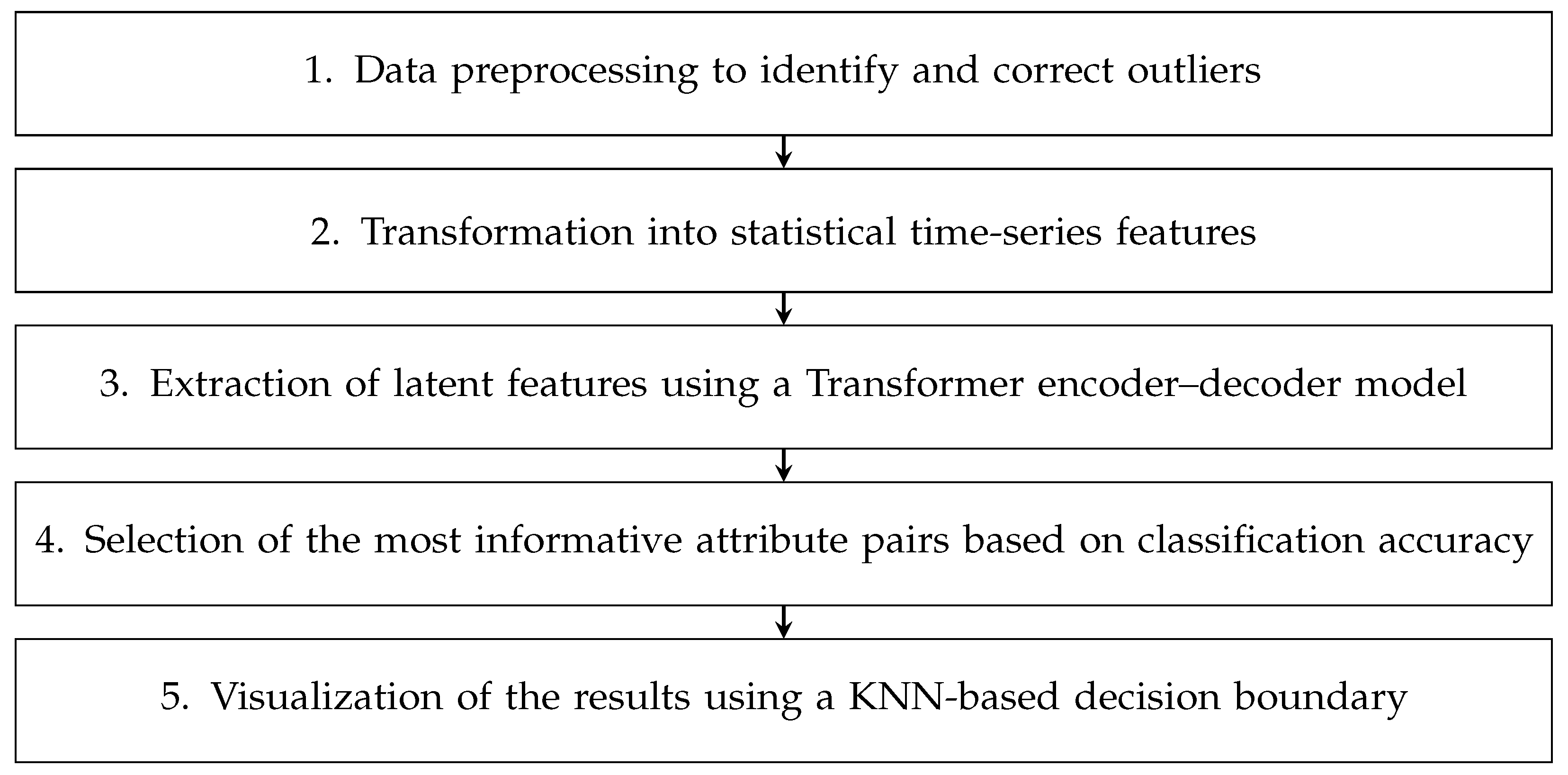
This study consists of three sections, which aim to evaluate the performance of the steam trap predictive maintenance system:

• Data acquisitions.
• Experiment setting.
• Performance evaluation.

Data collection was carried out by building a sensor network in two actual factories and receiving process data from the factories, and the experiment was conducted by building a machine learning operations (MLOps) environment. Finally, the performance evaluation was performed in three ways. First, the fault diagnosis performance of various machine learning models was measured and compared. Second, the clustering performance of the two-dimensional diagnostic projection generated by various characteristic factors was compared. Finally, the experiment was conducted to compare the thermal energy efficiency of a steam system scheduled for maintenance based on fault diagnosis with that of a steam system in its existing state and to input the effect of the scheduled maintenance system.

4.1. Data Acquisitions

Data for the experiment were obtained by installing sensors in large-scale aluminum processing plants and food manufacturing plants and performing precise diagnostics to secure learning data. Temperature sensors were strategically placed with the assistance of steam trap maintenance engineers at each plant and external steam trap experts. The training dataset was created by collecting work schedule data, including factory operating hours and planned maintenance (PM) dates, as well as temperature and humidity levels inside the factories, external weather conditions, the steam system configuration, and the purpose of steam-utilizing facilities. Additionally, temperature sensors were installed in the steam traps with the help of professional engineers.

We removed and corrected outliers from the sensor data to ensure data quality. Outliers were primarily identified using the 1.5 × IQR (Interquartile Range) rule, and additional criteria were applied, such as detecting values that remained unchanged up to the second decimal place for extended periods. Detected outliers were removed and corrected using the nearest neighbor interpolation method to maintain data continuity.

Furthermore, during the data validation process, we discovered that due to wireless sensor malfunctions, the inlet and outlet temperature values were swapped in some cases. To address this issue, we carefully analyzed the recorded data, identified incorrect assignments, and restored the proper order of temperature values. This correction allowed us to recover and ensure the integrity of the collected data. To improve fault diagnosis accuracy, we conducted a multi-step validation process. First, a primary fault diagnosis was performed based on the collected data. For cases where the diagnosis was unclear, a secondary on-site diagnosis was conducted using a portable thermal imaging camera in collaboration with factory engineers and external experts. Finally, for certain steam traps, a detailed inspection was performed by physically disassembling them, verifying the results of the secondary diagnosis, and completing the labeling of the acquired data.

The training data used for fault diagnosis and reliability assessment are presented in

Table 2. This table presents examples of training data used for fault diagnosis and reliability assessment visualization. It contains statistical time-series data, steam trap specifications, internal factory temperature, external weather information, and calendar data.

Attribute	Example 1	Example 2	Attribute	Example 1	Example 2
site_id	919	919	outlet_rms	97.79	97.806
dev_id	630	630	outlet_mean	97.79	97.806
dev_size	1	1	outlet_std	0.123	0.218
dev_type	0	0	outlet_skewness	0.082	0.439
dev_manufacturer	0	0	outlet_kurtosis_value	−1.18	−0.865
inlet_max	154.27	152.7	outlet_variance	0.015	0.047
inlet_min	147.81	148.53	outlet_wave_factor	1	1
inlet_absolute_average	151.744	150.49	outlet_clearance_factor	0.01	0.01
inlet_ptp	6.46	4.17	outlet_impulse_factor	1.002	1.005
inlet_rms	151.752	150.495	outlet_percentile25	97.7	97.633
inlet_mean	151.744	150.49	outlet_percentile50	97.785	97.81
inlet_std	1.564	1.284	outlet_percentile75	97.91	97.975
inlet_skewness	−0.755	−0.013	outlet_percentile90	97.94	98.129
inlet_kurtosis_value	−0.018	−1.296	outlet_sum_value	2346.96	2347.35
inlet_variance	2.445	1.648	outlet_median	97.785	97.81
inlet_wave_factor	1	1	env_temp	15.907	17.545
inlet_clearance_factor	0.007	0.007	env_humi	23.669	28.493
inlet_impulse_factor	1.017	1.015	outdoor_humi	67.324	71.406
inlet_percentile25	150.72	149.222	outdoor_temp	−1.251	1.013
inlet_percentile50	152.125	150.315	outdoor_feellike	−3.367	0.95
inlet_percentile75	152.888	151.538	outdoor_windspeed	1.867	0.779
inlet_percentile90	153.187	152.048	year	2024	2024
inlet_sum_value	3641.85	3611.75	month	1	1
inlet_median	152.125	150.315	day	3	10
outlet_max	98.02	98.26	weekday	3	3
outlet_min	97.6	97.49	operation	1	1
outlet_absolute_average	97.79	97.806	pm 1	0	0
outlet_ptp	0.42	0.77	label	4	4

¹ pm: Planned maintenance.

; various environmental and operational parameters are included.

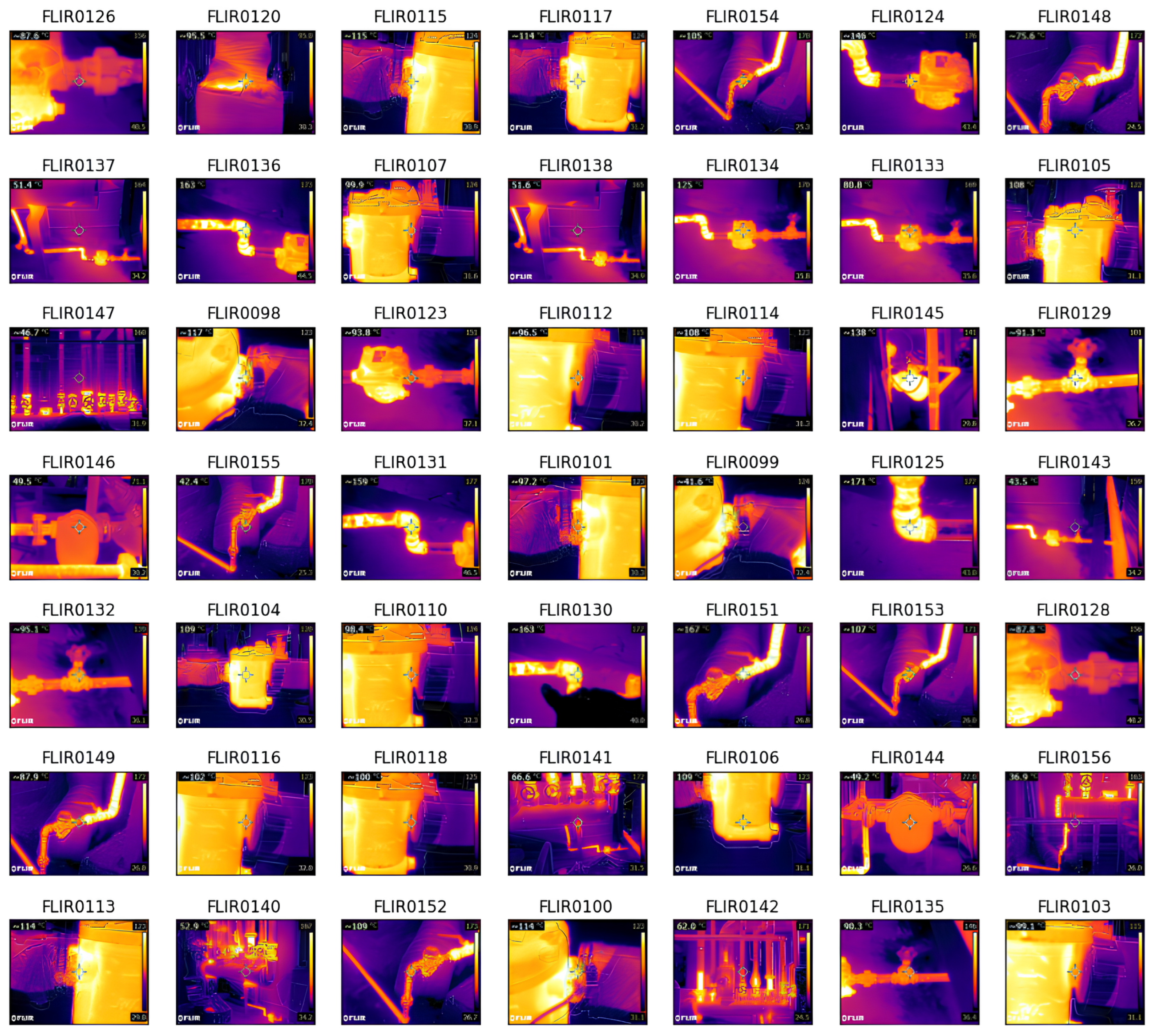
Figure 2 illustrates the thermal imaging of steam traps, which provides a visual representation of the temperature distribution across the main equipment in the steam system.

4.2. Experiment Settings

We acquired data from two factories to build experimental data and conducted a performance experiment on two-dimensional diagnostic projection, which can verify the reliability of the fault detector and fault diagnostic.

All data were collected online using the Industrial IoT platform. Some data were extracted from documents and worksheets and stored on the platform. Sensor data collection was performed at five-minute intervals and the other data were sampled at the same interval to build a training dataset. Afterwards, factory engineers and external experts worked on labeling the fault diagnosis and status.

Performance evaluation was performed by measuring the following evaluation indicators using 5-fold stratified cross-validation, where the data were split into folds while preserving the class distribution.

• Area Under Curve (AUC).
• Classification accuracy (CA).
• F-score (F1).
• Precision.
• Recall.

In this paper, the Transformer model and the machine learning and deep learning models below were compared with regard to their performance with the training data under the same conditions.

A performance evaluation of the two-dimensional diagnostic projection was conducted by comparing the distance between clusters and the dispersion of clusters, using the following cluster performance measurement indicators:

• Within-Cluster Sum of Squares (WCSS): Measures the compactness of clusters by calculating the sum of squared distances between each data point and the centroid of its assigned cluster. Lower values indicate tighter, well-defined clusters.
• Bayesian Information Criterion (BIC): Evaluates the trade-off between model complexity and goodness of fit. Lower values indicate better clustering performance with minimal overfitting.
• Davies–Bouldin Index (DBI): Assesses cluster separation and compactness by comparing intra-cluster dispersion with inter-cluster distances. Lower values indicate better-defined clusters.
• Adjusted Rand Index (ARI): Measures clustering accuracy by comparing the agreement between predicted clusters and ground truth labels. Higher values indicate stronger alignment with actual fault patterns.
• Calinski–Harabasz Index (CHI): Computes the ratio of between-cluster dispersion to within-cluster variance. Higher values indicate well-separated clusters with minimal overlap.

Table 3. Hyperparameter settings for the models used in the experiments.

Model	Hyperparameter	Value
Random Forest (RF)	Number of Trees	100
	Attributes Considered per Split	5
Gradient Boost (GB)	Number of Trees	100
	Learning Rate	0.1
	Max Depth per Tree	3
Adaptive Boosting (AdaBoost)	Number of Estimators	50
	Learning Rate	1.0
	Classification Algorithm	SAMME.R
	Regression Loss Function	Linear
Multi-layer Perceptron (MLP)	Network Structure	50 × 50 × 50
	Activation Function	ReLU
	Optimizer	Adam
Transformer (Ours)	Input Dimension	52
	Hidden Dimension	8
	Output Dimension	52
	Number of Layers	4
	Attention Heads	8
	Intermediate Size	32 (Hidden Dim × 4)
	Dropout Probability	0.1
	Max Sequence Length	512
	Optimizer	Adam (lr = ${10}^{-4}$)
	Loss Functions	MSE (Reconstruction), BCE (Classification)

presents the hyperparameter settings for the models utilized in our experiments. The optimal hyperparameters for each model were determined using RGHL (Rapid Genetic Exploration with Random-Direction Hill-Climbing for Linear Exploitation), a hyperparameter optimization technique that combines genetic algorithms with local search strategies to efficiently explore and exploit the hyperparameter space. This approach enables rapid convergence to near-optimal solutions while maintaining a balance between exploration and exploitation. The optimized values for each model are summarized in Table 3 [25].

4.3. Performance Evaluation

The performance evaluation of the fault diagnosis was conducted using a merged dataset, which integrates data from both the aluminum processing plant and the food manufacturing plant. To ensure unbiased evaluation, attributes that could identify the factory, such as the factory name, were removed before conducting the experiment.

Table 4. Fault diagnosis model performance evaluation. The best scores for each metric are highlighted in bold.

Model	AUC	CA	F1	Precision	Recall
RF	0.890	0.875	0.875	0.875	0.875
MLP	0.902	0.895	0.898	0.900	0.899
GB	0.906	0.887	0.886	0.888	0.887
AdaBoost	0.915	0.901	0.902	0.901	0.902
Transformer	0.927	0.932	0.938	0.916	0.914

compares fault diagnosis performance across models using AUC, CA, F1-score, Precision, and Recall. The Transformer model outperforms all others, achieving the highest AUC (0.927), CA (0.932), and F1-score (0.938), demonstrating its superior diagnostic capability. While AdaBoost and Gradient Boosting perform well, they fall short of the Transformer, confirming the effectiveness of deep learning-based fault detection.

Figure 3 illustrates the Receiver Operating Characteristic (ROC) curves for the Transformer-based fault diagnosis model, evaluating its ability to classify steam trap conditions into four categories: Unused (Class 0), Leaked (Class 1), Normal (Class 2), and Blocked (or closed valve) (Class 3).

Each solid line represents the ROC curve of an individual class, with the area under the curve (AUC) values indicated in the legend. The model achieves high AUC scores for all classes, with Class 0 and Class 1 reaching 0.93, while Class 2 and Class 3 achieve 0.91, indicating strong classification performance.

Additionally, the micro-average ROC curve (AUC = 0.92) and the macro-average ROC curve (AUC = 0.93) provide aggregated performance metrics, showcasing the model’s overall classification effectiveness across multiple fault types. The diagonal dashed line (y = x) represents the random classifier baseline, against which the model’s superior predictive capability is evident.

This result demonstrates the robustness of the Transformer model in identifying different fault conditions in steam traps, aiding in effective predictive maintenance and operational optimization.

While the current model demonstrates stable performance across different cross-validation folds, we anticipate that as more data become available, the stability of cross-validation results will further improve. This expectation is based on well-established statistical principles in machine learning, where larger datasets tend to reduce variance in model performance across different subsets of data.

Future research will aim to verify this hypothesis by incorporating additional sensor data from multiple industrial sites, analyzing the relationship between training data size and cross-validation robustness.

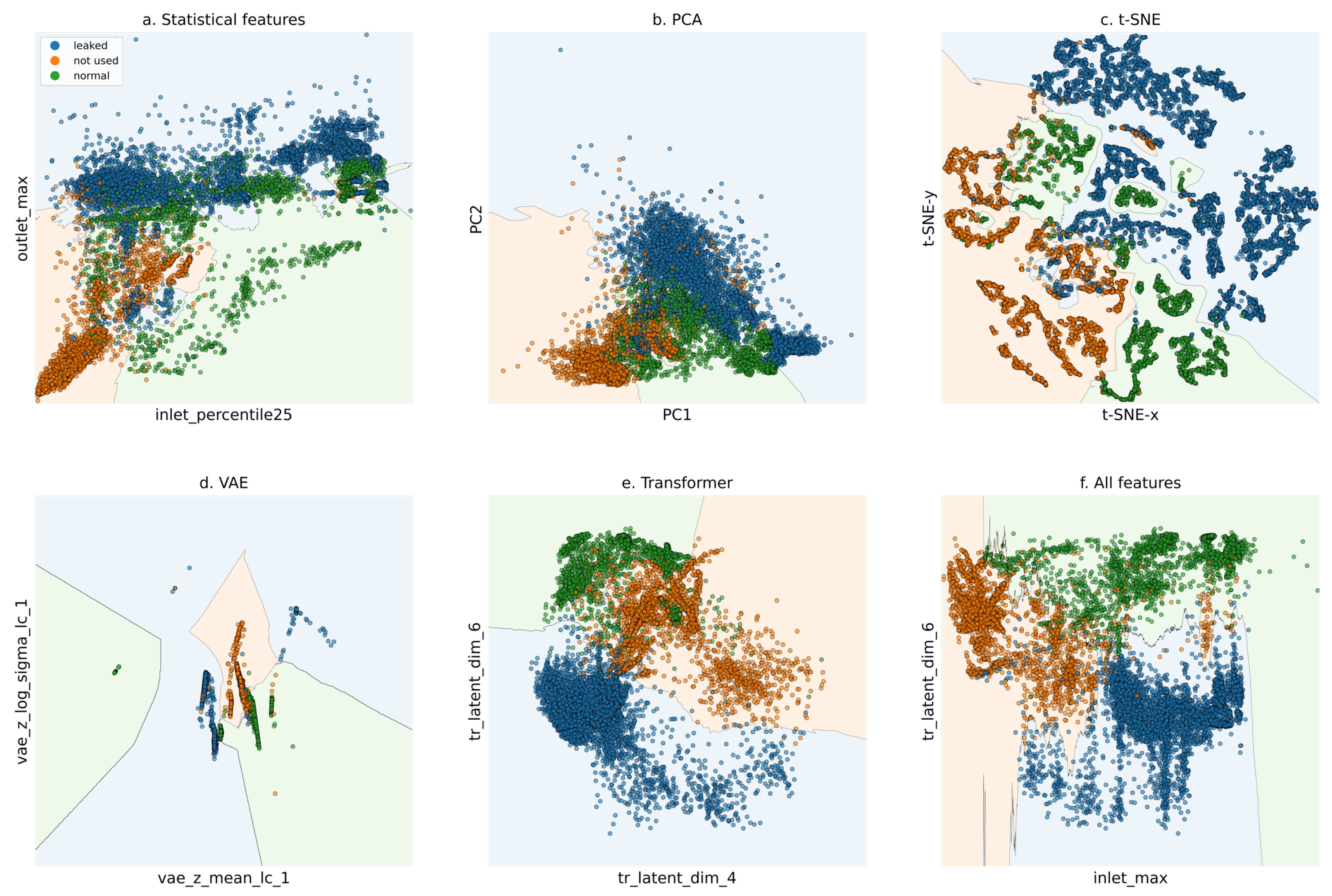
Figure 4 shows a visualization of the performance evaluation of the two-dimensional diagnostic projection, illustrating different methods from (a) to (f). (a) represents the visualization using simple statistics, providing a basic statistical perspective on the data distribution; (b) applies Principal Component Analysis (PCA) to reduce dimensionality while maintaining the overall variance of the dataset; (c) utilizes t-Distributed Stochastic Neighbor Embedding (t-SNE) to highlight local relationships within the data; (d) employs a Variational Autoencoder (VAE) to extract latent representations and project them into two dimensions; (e) presents the Transformer-based diagnostic projection, which shows a more stable distribution and clear decision boundaries between clusters compared to other visualizations, minimizing overlap between clusters. Finally, (f) combines all the properties from (a) to (e) to create a comprehensive visualization.

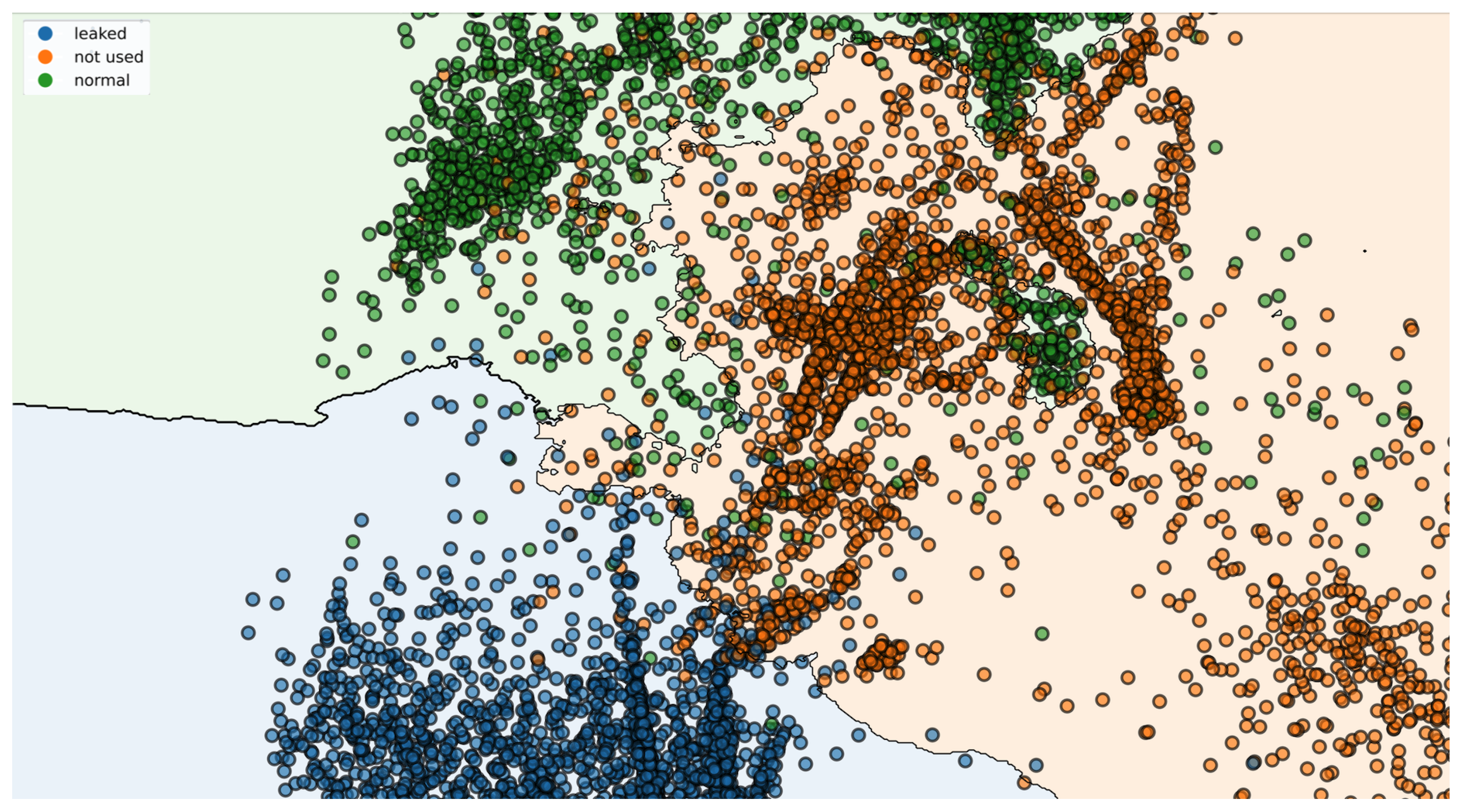
Figure 5 provides a detailed view of the overlapping regions in panel e of Figure 4, showing that the normal (green) and leaked (blue) clusters are relatively well separated. While some overlap between the normal and leaked clusters with the unused clusters is observed, it is considered negligible, as it does not significantly impact the diagnostic results.

Table 5. Comparison of clustering quality metrics for fault diagnosis models. The best scores for each metric are highlighted in bold.

Model	WCSS	BIC	DBI	ARI	CHI
Simple stats. 1	212,077	212,077	2.6145	0.7671	5392
PCA	169,806	103,608	2.2582	0.7479	5146
t-SNE	12,083,970	217,808	1.7633	0.8868	3579
VAE	7117	−33,338	1.8366	0.7421	1862
Transformer	19,700	74,711	0.8808	0.9195	14,558
All Features	8,638,854	161,006	4.1308	0.9256	11,738

¹ Simple stats.: Simple statistics.

demonstrates that the Transformer model delivers the best overall clustering quality, achieving the lowest DBI, a high ARI, and the highest CHI, ensuring that clusters are well separated and cohesive. The All Features model has the highest ARI but struggles with cluster separation, and the VAE model performs well in terms of compactness (WCSS) but lacks separation (low CHI). These results highlight the effectiveness of our proposed model for fault diagnosis in steam trap predictive maintenance.

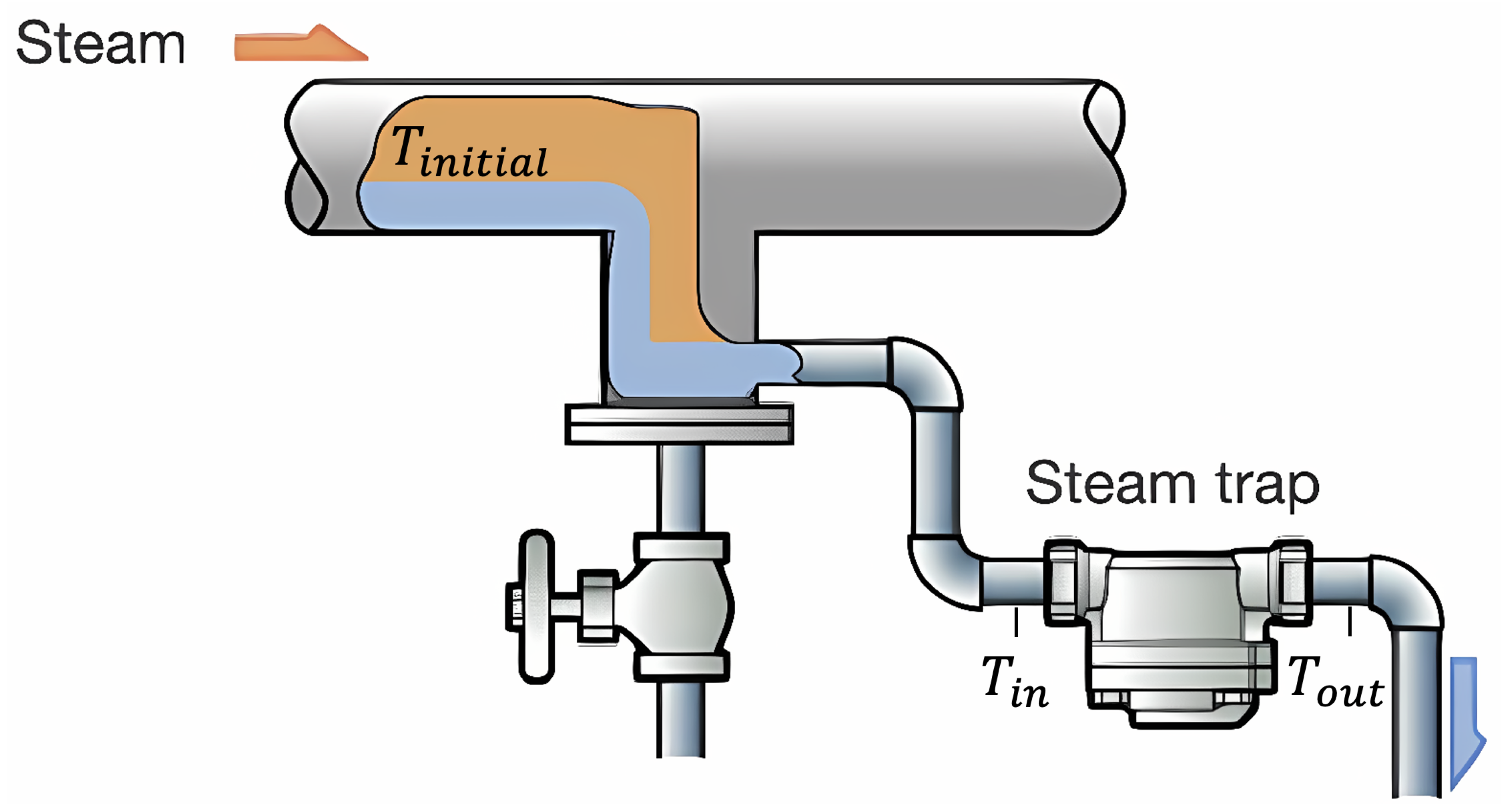
Figure 6 is referenced from the Miyawaki Inc. Steam Trap description article [26] and shows the structure of the steam trap and the temperature measurement location. It shows the temperature $(T_{initial}$) inside the steam pipe, the temperature ($T_{in}$) at the input of the steam trap, and the temperature ($T_{out}$) at the output of the steam trap in the steam system.

The thermal energy efficiency ($\eta$) is calculated as the ratio of the useful energy output to the total energy input, as shown in Equation (1):

$$\eta ={\displaystyle \frac{\mathrm{Useful}\mathrm{Energy}\left(\mathrm{Output}\right)}{\mathrm{Total}\mathrm{Energy}\left(\mathrm{Input}\right)}}\times 100$$

(1)

In the case of a steam system, the thermal energy efficiency can be expressed as follows:

$$\eta ={\displaystyle \frac{T_{initial}-T_{out}}{T_{initial}}}\times 100$$

(2)

To evaluate the impact of the predictive maintenance system, we define the thermal energy efficiencies before ($E_b$) and after ($E_a$) the system’s implementation. These are calculated as follows:

$$\begin{array}{cc}\hfill E_b& ={\displaystyle \frac{1}{t}}·\sum _{i=1}^t{\displaystyle \frac{T_{initial}-T_{out,i}}{T_{initial}}},\hfill \end{array}$$

(3)

$$\begin{array}{cc}\hfill \hspace{1em}\hspace{1em}\hspace{1em}\hspace{1em}\hspace{1em}\hspace{1em}{E}_a& ={\displaystyle \frac{1}{n-(t+\alpha +1)}}·\sum _{i=t+\alpha +1}^n{\displaystyle \frac{T_{initial}-T_{out,i}}{T_{initial}}}.\hfill \end{array}$$

(4)

Here, the variables are defined as follows:

• $T_{initial}$: Initial steam temperature at 1 atmosphere of pressure.
• $T_{out,i}$: Discharge temperature at the steam trap for the i-th measurement.
• t: The time point when the predictive maintenance system is introduced.
• $\alpha$: The installation period for the predictive maintenance system.
• n: The total number of data points.

The thermal energy efficiency before ($E_b$) is calculated using the average efficiency over the data collected prior to the system’s implementation. Similarly, the thermal energy efficiency after ($E_a$) is computed using the data collected after the installation and stabilization period ($t+\alpha +1$). By comparing $E_b$ and $E_a$, the effectiveness of the predictive maintenance system can be quantitatively evaluated.

$$\begin{array}{cc}\hfill E_{\mathrm{saving}}& =(E_{\mathrm{a}}-E_{\mathrm{b}})·100\approx {\displaystyle \frac{E_{\mathrm{a}}-E_{\mathrm{b}}}{max(E_{\mathrm{a}},E_{\mathrm{b}})}}·100\hfill \end{array}$$

(5)

We measured the thermal energy savings with the data obtained before and after the introduction of the predictive maintenance system at the two plants. The aluminum processing plant achieved an energy-saving rate of 7.2%, and the food manufacturing plant achieved 5.772%, for an average energy saving rate of 6.92%.

4.4. Computational Efficiency Analysis

To evaluate the computational efficiency of our Transformer-based fault diagnosis model for steam traps, we analyzed both training and inference times on different hardware configurations. This section presents a comparative analysis of CPU and GPU performance, highlights potential optimization strategies, and discusses the implications for large-scale deployment.

4.4.1. Dataset and Experimental Setup

We used training data collected from 50 steam traps in two industrial plants over one year, generating statistical time-series features daily. This resulted in approximately 180,000 data points. Execution time measurements were recorded during training.

Each experiment was repeated 100 times to ensure robustness and response times were analyzed with a confidence interval of 95%.

4.4.2. Hardware Specifications

The computational experiments were conducted using the hardware specifications listed in

Table 6. Hardware specifications for computational efficiency measurement.

CPU Specifications		GPU Specifications
Model	Intel Core i9-10920X	Model	NVIDIA GeForce RTX 3090 (x2)
Architecture	x86_64 (64-bit)	CUDA Cores	10,496 per GPU
Cores/Threads	12 Cores/24 Threads	Memory	24 GB GDDR6X per GPU
Base Clock	3.50 GHz	Memory Bandwidth	936.2 GB/s
Max Clock	4.80 GHz	Base Clock	1.40 GHz
L1 Cache	384 KiB	Boost Clock	1.70 GHz
L2 Cache	12 MiB	TDP	350 W per GPU
L3 Cache	19.3 MiB	CUDA Version	12.1
TDP	165 W	Driver Version	530.30.02
SIMD Extensions	AVX512, SSE4.2, FMA3
Virtualization	VT-x Supported

. The training and inference processes were tested on both a high-performance CPU (Intel Core i9-10920X) and a multi-GPU system (dual NVIDIA GeForce RTX 3090).

4.4.3. Training and Inference Performance

Table 7. Training and inference response times with 95% confidence interval.

Device	Train (s)	Inference (s)
CPU	$5.250\pm 0.057$	$0.0153\pm 0.00038$
GPU	$3.682\pm 0.029$	$0.0109\pm 0.00032$

presents the training and inference response times along with their 95% confidence intervals. The GPU setup demonstrated a significant reduction in training time compared to the CPU setup, resulting in a 29.9% improvement. Similarly, inference speed was improved by 28.7%, which is particularly beneficial for real-time fault diagnosis in industrial environments.

The improved performance of GPUs can be attributed to their parallel processing capabilities, which accelerate matrix multiplications and self-attention operations in Transformer-based architectures. However, it is important to note that CPU-based inference may still be a viable option for edge computing applications when GPUs are unavailable.

4.4.4. Scalability and Optimization Strategies

Based on the results from Table 7, several optimization strategies can be considered for large-scale deployment:

• Mixed-Precision Training: Leveraging FP16 computations using NVIDIA’s Automatic Mixed Precision (AMP) can further reduce memory consumption and improve training speed.
• Model Pruning and Quantization: Reducing model size by removing redundant parameters or converting weights to less precise formats (e.g., INT8) can enhance efficiency, especially for embedded systems.
• Distributed Training: Using multi-GPU training strategies such as model parallelism and data parallelism can scale up training for large industrial datasets.

5. Conclusions

This study proposed a deep learning model-based fault diagnosis framework for steam trap monitoring, demonstrating superior clustering performance and enhanced interpretability compared to traditional methods. By leveraging statistical time-series transformation and latent feature extraction, the model improves diagnostic accuracy and reliability through effective fault pattern identification.

Extensive experiments were conducted in two distinct industrial environments—an aluminum processing plant and a food manufacturing plant—where the system exhibited strong adaptability and robustness. The results indicated average thermal energy savings of 6.92% across both sites, underscoring its potential to reduce energy consumption and greenhouse gas emissions. Additionally, the implementation of a two-dimensional diagnostic projection significantly improved interpretability, enabling maintenance engineers to prioritize repairs more effectively and ensure operational reliability.

While the results are promising, several limitations must be addressed:

• Data Availability: The model requires a large labeled dataset, which may not always be feasible in industrial environments.
• Energy Consumption Variability: External factors such as production schedules, seasonal changes, and maintenance activities may impact energy savings. Additional studies are needed to analyze these influences.
• Sensor Dependency: The current approach primarily relies on temperature data, limiting applicability to diverse steam trap configurations. Future work should explore multimodal sensor integration (e.g., pressure and acoustic signals).
• Model Comparison: While the proposed Transformer-based model outperformed traditional machine learning methods, this study did not include a direct comparison with self-supervised learning approaches. Future work will explore the integration of self-supervised models, which can leverage unlabeled data to reduce labeling costs and enhance scalability. Comparing these models will provide insights into their relative performance, computational efficiency, and cost-effectiveness.
• Cost–Benefit Analysis: Although this study analyzed the energy-saving potential of the proposed system, a comprehensive cost–benefit analysis was not conducted. Future research will incorporate an economic assessment that considers installation and operational costs alongside energy savings to evaluate the financial feasibility of this AI-driven predictive maintenance system.

Moving forward, we plan to expand this approach in several key areas. One potential direction is domain adaptation, which will allow us to deploy the model across diverse industrial settings with varying steam trap configurations. Conducting tests in multiple factories will help assess its generalizability and adaptability. Additionally, integrating multimodal sensor data will reduce dependency on a single sensor type, enhancing reliability in complex industrial environments. Lastly, extending this framework beyond steam traps to other industrial equipment will validate its applicability to broader predictive maintenance applications. These advancements will contribute to a more scalable and practical predictive maintenance system.

In conclusion, while the proposed method significantly improves fault diagnosis and energy efficiency, further research is needed to refine its adaptability, validate long-term energy savings, and enhance its applicability across diverse industrial conditions. Moreover, incorporating a cost–benefit analysis will be crucial to assess the method’s economic feasibility and promote its adoption in real-world industrial applications. Future studies will also investigate self-supervised models to reduce the reliance on labeled data and improve scalability, offering a broader perspective on model efficiency and deployment in a range of industrial settings.