Optimization of Oil Well Production Prediction Model Based on Inter-Attention and BiLSTM

Abstract

Accurate prediction of future oil production is critical for decision-making in oil well operations. However, existing prediction models often lack precision due to the vast and complex nature of oil well data. This study proposes an oil well production prediction model based on the Inter-Attention Mechanism (IAM) and Bidirectional Long Short-Term Memory Network (BiLSTM), optimized using a Comprehensive Search Algorithm (CSA). By incorporating the Inter-Attention Mechanism, the model enhances its capacity to model complex time-series data. The CSA, combined with Sequential Quadratic Programming (SQP) and Monotone Basin Hopping (MBH) algorithms, ensures both global and local parameter optimization. Using historical data from an oil well in Sichuan, the feasibility of the proposed model was validated, demonstrating superior accuracy and robustness compared to other prediction models and optimization algorithms.

1. Introduction

In the process of oil production, oil well production prediction is typically conducted to save time and resources in detecting well production, as well as to comprehensively evaluate and prepare for well development [1]. However, current oil well production predictions face challenges, such as suboptimal performance and insufficient model generalization [2], making efficient and accurate predictions difficult and impacting the scientific quality of production decisions and optimal resource allocation.

With the development of oil field technology and artificial intelligence, scholars, both domestically and internationally, have conducted extensive research on oil well production prediction [3]. Traditional prediction methods, such as empirical formula methods [4], curve fitting methods [5], and numerical simulation methods [6], suffer from excessive reliance on experience, complex computations, and poor adaptability. In the field of oil well production prediction, traditional methods primarily rely on physical-based models and empirical formulas [7]. These methods typically involve analyzing key parameters such as reservoir fluid flow, reservoir pressure, and geological characteristics, combined with historical production data, to establish mathematical models for prediction [8]. Common models include capacity equations, pressure recovery analysis, and material balance methods. For example, Van Everdingen A. F. explored the use of the Material Balance Equation (MBE) as a predictive tool for estimating future production [9], while Xu J reviewed the development of reservoir simulation methods [10], highlighting their importance in predicting oil well performance. The advantage of these methods lies in their solid physical foundation, making them particularly suitable for cases with limited early data.

In the field of reservoir engineering, oil well production prediction via artificial intelligence prediction methods has been widely applied in recent years, mainly including machine learning and deep learning techniques. These methods train on large amounts of historical production data, automatically mining potential nonlinear relationships, and are capable of effectively capturing dynamic changes under complex working conditions and multi-factor coupling. Common algorithms include Convolutional Neural Networks (CNN), Random Forest (RF) [11], Long Short-Term Memory Networks (LSTM) [12], and ensemble models [13]. These methods do not rely on detailed physical model support and, when sufficient data is available, can significantly improve prediction accuracy, although they have higher requirements for data quality and quantity.

Deep learning methods have demonstrated especially strong performance in handling large-scale data and intricate nonlinear relationships. For example, research based on the GRU-KAN model improved prediction accuracy and efficiency by combining Gated Recurrent Units (GRU) and Kernel Attention Networks (KAN) [14]; probabilistic machine learning methods were used to quantify the uncertainty in the prediction process, thereby improving the profitability of oil and gas wells [15]; prediction models combining Principal Component Analysis (PCA) and GRU improved the accuracy of oil well production predictions [16]; and data-driven regression models developed using sequential convolution and Long Short-Term Memory (LSTM) units have been applied to oil production forecasting, achieving high prediction accuracy [17]. However, most of these studies lack optimization of the prediction models, leading to deficiencies in accuracy, efficiency, and adaptability, especially the tendency to fall into local optima, which impacts prediction accuracy.

Traditional methods (such as the empirical formula method and numerical simulation method) are difficult to adapt to the dynamic changes of the reservoir environment due to complex calculations and high data dependence. Artificial intelligence methods (especially deep learning) have gradually become an important means of oil well production prediction due to their powerful data processing capabilities. However, the current deep learning model still has shortcomings in prediction accuracy, generalization ability, and avoiding local optimality. Therefore, this paper proposes an oil well production prediction model based on IAM-BiLSTM and optimizes it through a Comprehensive Search Algorithm (CSA) to improve prediction accuracy and stability. First, by combining the Inter-Attention Mechanism with the BiLSTM structure, the IAM-BiLSTM model is designed to more effectively filter and retain key features, thereby improving prediction accuracy. Second, the paper introduces a CSA algorithm that combines the Monotone Basin Hopping Algorithm (MBH) and Sequential Quadratic Programming (SQP) algorithm, optimizing the model parameters through the global search ability of MBH and the local optimization ability of SQP. Finally, experimental results demonstrate that the IAM-BiLSTM model optimized by CSA significantly outperforms traditional methods in prediction performance.

2. Methodology

This chapter introduces the proposed IAM-BiLSTM model and the CSA optimization algorithm. First, it presents a BiLSTM-based prediction model incorporating an Inter-Attention Mechanism and explains its working principles. Then, it describes the CSA algorithm, which combines MBH and SQP, along with its improvement strategies.

2.1. IAM-BiLSTM Model

2.1.1. Inter-Attention Mechanism

The Inter-Attention Mechanism is a data processing method in machine learning [18], widely applied in tasks such as natural language processing [19], image recognition, and speech recognition [20]. The degree of focus on different pieces of information in the attention mechanism is reflected through weights [21]. The attention mechanism can be regarded as a multilayer perceptron (MLP) composed of a query matrix (Q), keys (K), and weighted averages (V).

The Inter-Attention Mechanism is a type of attention mechanism in deep learning used to capture the correlations and interactions between two different sequences or datasets [22]. Its working principle is similar to that of the standard attention mechanism, with the difference being that one of the sequences is used as the Q, while the other sequence serves as the K and V. The corresponding attention weights and attention values are then calculated. The Inter-Attention Mechanism can effectively model the dependencies between two distinct sequences, thereby enhancing the model’s understanding of the input data.

2.1.2. BiLSTM Model

Standard Recurrent Neural Networks (RNNs) capture only limited contextual information in sequential tasks [23]. To address this, Long Short-Term Memory (LSTM) introduces cell states and gating mechanisms—forget gate, input gate, and output gate—each controlled by the sigmoid function [24]. However, conventional LSTMs may still ignore future context. Bidirectional LSTMs (BiLSTMs) [25] solve this issue by running two LSTMs in opposite directions and combining their outputs, thus incorporating both past and future information.

Concretely, for a BiLSTM network, the output at time $t$, $y_t,$ is determined by the forward state $h_t$, the backward state $h_t^{\prime }$, and the input $x_t$. The update formulas are:

$$\begin{array}{l}{h}_t=z_1\left({\omega }_1{x}_t+{\omega }_5{h}_{t-1}\right)\\ h_t^{\prime }=z_2\left({\omega }_2{x}_t+{\omega }_6{h}_{t+1}^{\prime }\right)\\ y_t=z_3\left({\omega }_3{h}_t+{\omega }_4{h}_t^{\prime }\right)\end{array}$$

(1)

where ${\omega }_i(i=\mathrm{1,2},\cdots ,6)$ is the corresponding weight of each layer and $z_i(i=1,2,3)$ is the activation function of different layers.

2.1.3. IAM-BiLSTM Prediction Model

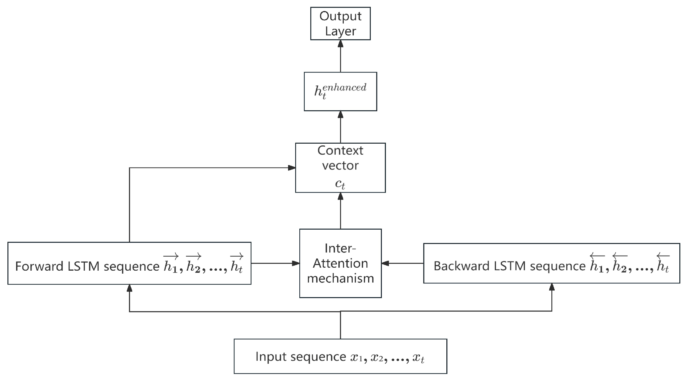
By introducing an Inter-Attention Mechanism between the forward and backward LSTMs, the forward and backward LSTMs are able to “attend” to each other’s hidden states at each time step, thereby better capturing the bidirectional dependencies within the sequence. Table 1 outlines the implementation steps of the IAM-BiLSTM prediction model.

Table 1. IAM-BiLSTM Prediction Model Implementation Steps.

Step 1: Given the input sequence $\left\{x_1,x_2,\dots ,x_T\right\}$, the forward LSTM computes the hidden states $\left\{{\overrightarrow{h}}_1,{\overrightarrow{h}}_2,\dots ,{\overrightarrow{h}}_T\right\}$ from t = 1 to T, and the backward LSTM computes the hidden states $\left\{{\overleftarrow{h}}_1,{\overleftarrow{h}}_2,\dots ,{\overleftarrow{h}}_T\right\}$ from t = T to 1.

Step 2: Calculate the attention weights. For each time step t, compute the attention weight between the forward hidden state ${\overrightarrow{h}}_t$ and all backward hidden states $\left\{{\overleftarrow{h}}_1,{\overleftarrow{h}}_2,\dots ,{\overleftarrow{h}}_T\right\}$, use a compatibility function to calculate the similarity score: $e_{t,k}=\mathrm{s}\mathrm{c}\mathrm{o}\mathrm{r}\mathrm{e}\left({\overrightarrow{h}}_t,{\overleftarrow{h}}_k\right)$, and apply Softmax to the scores.

Step 3: Compute the context vector. Use the attention weights to calculate the context vector $c_t$, which is the weighted sum of the backward hidden states: $$c_t=\sum _{k=1}^T{\alpha }_{t,k}{\overleftarrow{h}}_k$$

Step 4: Combine the hidden state and context vector. Concatenate the forward hidden state ${\overrightarrow{h}}_t$ and the context vector $c_t$, forming an enhanced representation: $$h_t^{enhanced}=Concat({\overrightarrow{h}}_t,c_t)$$

Step 5: Use the enhanced representation $h_t^{enhanced}$ for subsequent tasks.

By incorporating the Inter-Attention Mechanism into BiLSTM, the forward and backward LSTMs can mutually attend to each other’s hidden states at each time step, enabling the capture of richer bidirectional information. A trainable feedforward network is used to compute the similarity scores, enhancing the model’s representational capacity. The context vector $c_t$, which summarizes the global information from the counterpart LSTM, aids in making more accurate predictions at the current time step. Figure 1 illustrates the IAM-BiLSTM prediction model.

Figure 1. Schematic Diagram of the IAM-BiLSTM Prediction Model.

2.2. Comprehensive Search Algorithm

In oil well production prediction based on artificial intelligence methods, incorporating optimization algorithms can effectively enhance the accuracy of prediction models. This interdisciplinary approach improves prediction accuracy and efficiency across various fields. Azevedo B. F. conducted a comprehensive review of hybrid methods combining optimization and machine learning techniques [26], including their applications in clustering and classification tasks. Krzywanski J. explored the applications of artificial intelligence and other advanced computational methods in energy systems [27], including material production and optimization. These studies collectively demonstrate that the use of optimization algorithms can significantly improve the performance of prediction models.

2.2.1. Sequential Quadratic Programming (SQP)

The Sequential Quadratic Programming (SQP) algorithm is a nonlinear optimization method that iteratively refines the solution by solving Quadratic Programming (QP) subproblems. In this study, SQP is integrated with the Monotone Basin Hopping (MBH) algorithm to enhance global optimization capabilities, addressing the limitations of conventional deep learning parameter tuning. SQP applies a quasi-Newton method to the Kuhn–Tucker conditions, where the Lagrangian function is given by Formula (2):

$$L\left(x,\lambda ,\mu \right)=f\left(x\right)+\sum _{i=1}^m{\lambda }_i{h}_i\left(x\right)+\sum _{j=m+1}^n{\mu }_j{g}_j\left(x\right)$$

(2)

where $x$ denotes the decision variable vector, $f\left(x\right)$ is the objective function, $h_i\left(x\right)$ and $g_j\left(x\right)$ represent the equality and inequality constraints, ${\lambda }_i$ and ${\mu }_j$ represent the equality and inequality constraints, $m$ is the number of equality constraints, and $n$ is the total number of constraints. In each iteration, the search direction $d$ is determined by solving the following QP subproblem:

$$\begin{array}{l}min1/2d^T{H}_{k}d+{\left(\nabla f\left(x_k\right)\right)}^{T}d\\ \mathrm{s}.\mathrm{t}.{\left(\nabla h_i\left(x\right)\right)}^{T}d+h_i(x)=0\\ {\left(\nabla g_j\left(x\right)\right)}^{T}d+g_j(x)=0\end{array}$$

(3)

The new solution is then updated by $x_{k+1}=x_k+a_k{d}_k$, where $a_k$ is obtained via a line search. The Hessian approximation $H_k$ is updated using the DFP formula:

$$H_{k+1}=H_k-{\displaystyle \frac{H_k{y}_k{y_k}^T{H}_k}{{y_k}^T{H}_k{y}_k}}+{\displaystyle \frac{s_k{s_k}^T}{y_k{s_k}^T{s}_k}}$$

(4)

where $y_k$ is the difference in gradients of the Lagrangian and $s_k$ is the difference in the solution estimates.

The steps of the SQP algorithm are shown in Table 2.

Table 2. SQP Algorithm Steps.

Step 1: Choose a feasible initial point $x_0$; set $k=0$.

Step 2: Iteration step (for each $k$): (1) Linearize the constraints and form the quadratic approximation of the Lagrangian. (2) Solve the QP subproblem for $d_k$. (3) Determine ${\alpha }_k$ and update $x_{k+1}=x_k+a_k{d}_k$. (4) Update Lagrange multipliers and the Hessian approximation $H_{k+1}$.

Step 3: If convergence criteria are met, stop; otherwise, increment $k$ and repeat.

2.2.2. Monotone Basin Hopping Algorithm (MBH)

The Monotone Basin Hopping Algorithm (MBH) is designed to find global optima in problems with many local minima [28]. It extends the Basin Hopping Algorithm (BH) by introducing a monotonicity constraint: if a new point has a lower objective value but violates the monotonicity condition (i.e., one of its variables is larger than that in the current best solution), it is rejected. MBH was originally developed for molecular conformation problems in computational chemistry [29], combining monotonic search and basin hopping to achieve global optimization.

MBH exhibits strong global search capabilities [30]. Unlike traditional local search algorithms that easily get trapped in local optima, MBH uses a basin hopping strategy to explore the solution space globally, thus improving the probability of finding the global optimum. Additionally, randomness helps discover potentially better solutions. The MBH steps are summarized in Table 3.

Table 3. MBH Algorithm Steps.

Step 1: Generate a randomly started local minimum $x_0$ and set the consecutive rejection counter $R$ to 0.

Step 2: From the current local minimum $x_k$, add a random perturbation $S$ to obtain $x_k+S$, then find a new local minimum Y by local minimization starting at this perturbed point. If $E\left(Y\right)<E\left(x_k\right)$, then accept $x_{k+1}=Y$. Reset the consecutive rejection counter $R$ to 0 and return to Step 1. Otherwise, reject $Y$ and increment $R$. If $R\le R_{max}$, retain $x_k$ and return to Step 1; if $R>R_{max},$ go to Step 3.

Step 3: Use the current $x_k$ as the bottom of the funnel and terminate the sequence.

2.2.3. Comprehensive Search Algorithm (CSA)

Although the MBH algorithm can help find the global optimum or near-optimal solutions, there is still the risk of getting stuck in local optima. Therefore, it is combined with the SQP algorithm. SQP has weak global search capabilities but strong local search capabilities, allowing it to converge to local extrema in a short time. By combining them, their strengths can complement each other. The integration of Sequential Quadratic Programming (SQP) and Monotone Basin Hopping (MBH) algorithms provides a comprehensive optimization method that combines both global and local search capabilities, known as the Comprehensive Search Algorithm (CSA), as shown in Figure 2. Its detailed steps are outlined in Table 4.

Figure 2. Comprehensive Search Algorithm (CSA) Flow Chart.

Table 4. CSA Algorithm Steps.

Step 1: Randomly generate an initial solution $x_0$, set the continuous rejection counter $R=0$, the maximum number of continuous rejections $R_{max}$, and the allowable error $ϵ$.

Step 2: For the current local minimum $x_k$, generate a random perturbation vector $S\in R^{3N}$ so that the new starting point is: $X_{new}=x_k+S$. Random perturbation vector: $S=\alpha ·U$.

Step 3: Use the sequential quadratic programming (SQP) algorithm to start the local optimal search for the new candidate point $X_{new}$ and obtain the new local minimum $Y$.

Step 4: Determine whether the new solution Y is better than the current solution x_k. If the objective function value $E\left(Y\right)<E\left(x_k\right)$, the new solution Y is considered to be a better solution, that is: $x_{k+1}=Y$. Reset the continuous rejection counter $R$ to 0. Return to Step 1.

Step 5: If the objective function value $\mathit{E}\left(\mathit{Y}\right)\ge \mathit{E}\left({\mathit{x}}_{\mathit{k}}\right),$ reject $\mathit{Y}$, i.e., $x_{k+1}=x_k$. Increase the consecutive rejection counter $R$ by 1.

Step 6: Determine whether the continuous rejection counter R reaches the maximum allowed value $R_{max}$. If $R\le R_{max}$, return to Step 2 and perform new random perturbations and local searches. If $R>R_{max}$, it is considered that the current solution cannot be further improved, and the loop is exited to enter the termination step.

2.3. CSA Optimization IAM-BiLSTM Prediction Model

This study uses the CSA to optimize the IAM-BiLSTM prediction model. First, historical data from a specific oil well in Sichuan is collected, and an IAM-BiLSTM prediction model is proposed. The historical data includes production data of each well, well pressure, wellhead temperature, separator pressure, separator temperature and manifold pressure. The CSA algorithm is then used to optimize the parameters of the prediction model. Finally, the optimized IAM-BiLSTM prediction model is applied to predict oil well production, and the prediction results are obtained. By comparing the results of the optimized IAM-BiLSTM model with other prediction algorithms, it is evident that the optimized IAM-BiLSTM prediction model demonstrates superior accuracy and feasibility in the field of oil well production prediction.

For the parameters of the proposed IAM-BiLSTM model that may influence prediction accuracy, this section employs the CSA to search for their optimal values to improve the model’s predictive performance. The optimization process for the IAM-BiLSTM model is illustrated in Figure 3, and the steps are detailed in Table 5.

Figure 3. CSA-Optimized IAM-BiLSTM Prediction Model.

Table 5. CSA Optimization IAM-BiLSTM Steps.

Step 1: The time series features with high correlation with production obtained in the well site are used as input variables of the prediction model. In order to avoid the large difference in magnitude of different variables affecting the accuracy of the model, the data samples are standardized: $X_{\mathrm{nom} }={\displaystyle \frac{X-X_{min}}{X_{max}-X_{min}}}\in [0,1]$.

Step 2: Initialize the model parameters $\theta (l_r,S_b,E_p,L_{out},c_1,c_2,c_3)$ to be optimized. Set the maximum number of rejections $R_x=20$ and the random perturbation amplitude of the model parameters.

Step 3: Given the training samples and model parameters, the oil well production prediction model is established using the above IAM-BiLSTM prediction model.

Step 4: Define the mean square error of the IAM-BiLSTM prediction model results as the loss function.

Step 5: Train the model using the new perturbed parameters and calculate the model loss $L_{new}$ after training.

Step 6: Perform local optimization on the perturbed parameters, retrain the model with the optimized parameters, and calculate the optimized model loss $L_{new}$.

Step 7: Determine whether to accept the new solution. If $L_{new}\le L_{best}$, accept the new solution, update the optimal parameters and loss function, and exit the optimization search. If $L_{new}>L_{best}$, reject the new solution and search for the best solution again.

3. Results and Discussion

In this section, we describe the experimental setup and compare the prediction results. In the experiments, the IAM-BiLSTM model is compared with the Back Propagation neural network (BP), Support Vector Machine (SVM), Extreme Gradient Boosting (XGBoost), BiLSTM, and AM-BiLSTM (Attention Mechanism-Bidirectional Long Short-Term Memory) for production prediction, and the comparative results are presented. Additionally, the results of optimizing the IAM-BiLSTM model using the Grey Wolf Optimizer (GWO) [31], Particle Swarm Optimizer (PSO) [32], and Whale Optimization Algorithm (WOA) [33] are compared with those obtained using the CSA-optimized model. The models used in the experiments were primarily implemented in Python 3.10.

3.1. Data Types

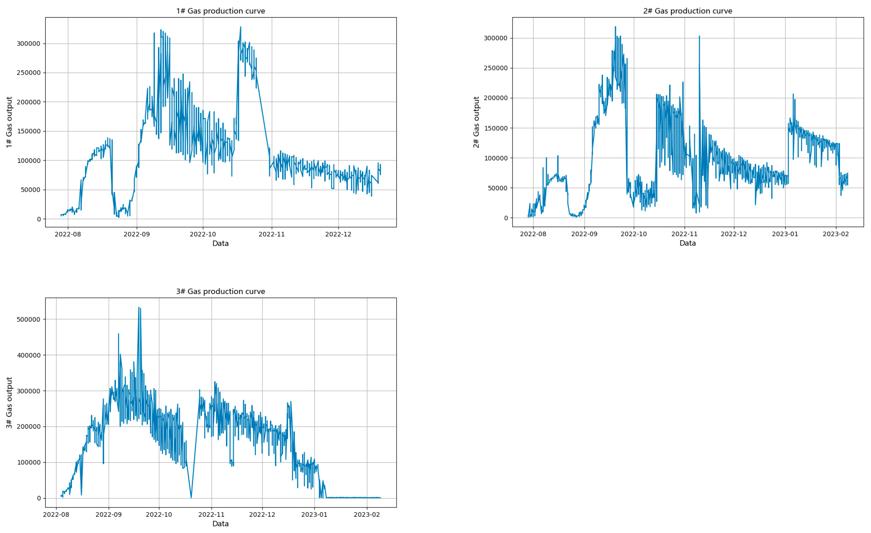
Based on the operating conditions of ground equipment and production equipment at a specific oil well site in Sichuan, the experimental data used consists of historical dynamic liquid level data collected on-site from three oil wells during 2021–2022. To enhance the generalization ability of the model, 1000 data points were randomly selected from each well to construct the dataset. Each dataset corresponds to dynamic liquid level data measured over a month for a specific well. The production variations for the three wells are shown in Figure 4 [34]. The standard deviation and variance reflect the fluctuation of a dataset, while the mean, minimum, and maximum values indicate the differences in production among the wells [35]. The standard deviation, minimum, and maximum values of the oil well production data are listed in Table 6. This dataset can be used to validate the proposed model’s performance in predicting wells with significant production disparities.

Figure 4. Production Changes of Three Oil Wells.

Table 6. Production of Three Wells in a Well Field.

Number of Wells	Mean	Standard Deviation	Variance	Maximum
1	122,525.45	90,270.89	8,148,835,259.10	435,133.1
2	76,886.25	73,732.17	5,436,433,284.58	346,582.5
3	220,579.66	71,483.74	5,109,925,865.95	591,495.4

3.2. Evaluation Criteria

This study uses the Mean Squared Error (MSE) and Mean Absolute Error (MAE) as evaluation metrics to comprehensively assess the predictive performance of the model. The smaller the values of these metrics, the closer the predicted values are to the actual values, indicating better prediction performance.

$$\mathrm{M}\mathrm{S}\mathrm{E}={\displaystyle \frac{1}{\mathrm{m}}}\sum _{\mathrm{i}=1}^{\mathrm{m}}{\left({\mathrm{y}}_{\mathrm{i}}-{\widehat{\mathrm{y}}}_{\mathrm{i}}\right)}^2$$

(5)

$$\mathrm{M}\mathrm{A}\mathrm{E}={\displaystyle \frac{1}{\mathrm{m}}}\sum _{\mathrm{i}=1}^{\mathrm{m}}\left|{\mathrm{y}}_{\mathrm{i}}-{\widehat{\mathrm{y}}}_{\mathrm{i}}\right|$$

(6)

where ${\mathrm{y}}_{\mathrm{i}}$ is the actual oil production value, ${\widehat{\mathrm{y}}}_{\mathrm{i}}$ is the predicted oil production value, and $\mathrm{m}$ is the total amount of oil production data in the test dataset.

3.3. Verifying the Effectiveness of the IAM-BiLSTM Prediction Model

3.3.1. Feature Engineering and Model Tuning

The proposed IAM-BiLSTM prediction model is designed for time series data. In addition to gas production, the dataset also includes well pressure, wellhead temperature, separator pressure, separator temperature, and manifold pressure. Data other than gas production are used as input features, and gas production is used as the target feature for prediction. The input features have been normalized to ensure consistency. We use the sliding window technique to convert the sequence data into feature-target pairs, making them suitable for training BP, SVM, and XGBoost models. The dataset is divided into 80% training and 20% testing to evaluate the model performance. In order to verify the improvement in prediction performance compared with machine learning methods, prediction models based on BP network, SVM, and XGBoost are established for comparison. The data collected from the three wellheads have the same characteristics, and all datasets are readings from field equipment sensors. The data characteristics are shown in Table 7.

Table 7. Oil Well Basic Statistics of Features.

Oil Well Number	Data Characteristics	Average Value	Standard Deviation	Data Unit
Well 1	Well pressure	137.2994	97.7015	MPa
	Wellhead temperature	29.0783	5.5435	°C
	Manifold pressure	33.3678	6.3404	MPa
	Separator pressure	3.3701	0.8442	MPa
	Separator temperature	81.7237	12.6625	°C
	Gas production	122,417.8197	90,081.2698	m3
Well 2	Well pressure	104.0779	75.2034	MPa
	Wellhead temperature	39.8731	11.9762	°C
	Manifold pressure	23.6309	15.1888	MPa
	Separator pressure	3.3957	0.9003	MPa
	Separator temperature	65.6631	14.1295	°C
	Gas production	100,100.3016	60,535.3192	m3
Well 3	Well pressure	107.7074	67.1752	MPa
	Wellhead temperature	34.0275	3.4423	°C
	Manifold pressure	28.9450	7.8847	MPa
	Separator pressure	3.7279	0.8624	MPa
	Separator temperature	86.5867	9.3566	°C
	Gas production	220,666.6295	71,503.8883	m3

Additionally, to evaluate the impact of the attention mechanism on the prediction model, BiLSTM and AM-BiLSTM models were also constructed for comparison. The network parameters of the prediction models involved in this study are shown in Table 8, where $I_{input}$ and $I_{output}$ represent the input and output for SVM, XGBoost, and the BP neural network, respectively, $C$ is the hyperparameter for SVM, with other parameters set to default values, $gamma$ is the optimization parameter for XGBoost, with other parameters also set to default values, and $c_i$ denotes the number of neurons in the i-th hidden layer. For BiLSTM, $L_{input}$ and $L_{output}$ represent the input and output, respectively. To validate the model’s accuracy, the training batch size $S_b$, learning rate $l_r$, loss function, and optimizer are kept consistent across models.

Table 8. Parameter Settings of the Comparative Prediction Models.

Prediction Model	Parameter Settings
BP	$I_{input}=438\times 1,C=3,I_{output}=1$
SVM	$I_{input}=438\times 1,gamma=0.1,I_{output}=1$
XGBoost	$I_{input}=438\times 1,c_1=512,c_2=128,c_3=32,c_4=8,I_{output}=1$
BiLSTM	$S_b=128,l_r=0.001, loss function: MSE, optimizer: Adam,$ $L_{input}=216\times 2,L_{output}=32\times 1,c_1=128,c_2=128,c_3=64,c_4=8$
AM-BiLSTM	$S_b=128,l_r=0.001,E_p=1000,loss function: MSE, optimizer: Adam, L_{input}=216\times 2,$ $L_{output}=32\times 1,c_1=128,c_2=128,c_3=64,c_4=8$

3.3.2. Verification Results

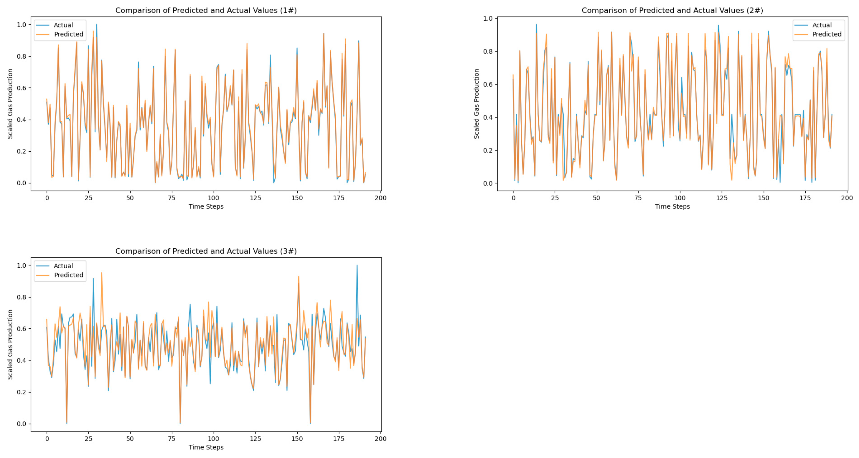
To verify the effectiveness of the proposed IAM-BiLSTM prediction model in the field of oil well production prediction, as well as the improvement in prediction accuracy brought by the Inter-Attention Mechanism to the BiLSTM model, production prediction models were established based on the aforementioned dataset and model parameters. The results of predicting oil well production using the IAM-BiLSTM prediction model are shown in Figure 5.

Figure 5. IAM-BiLSTM Model Prediction Results.

After comparing the prediction results with several machine learning and deep learning methods, Figure 6 was obtained, and the prediction accuracy calculation results are shown in Table 9. The results can be summarized as follows:

Figure 6. Prediction Results.

Table 9. Error Results of Different Prediction Methods.

Prediction Method	MSE	MAE
BP	0.0391	0.0945
SVM	0.0567	0.1077
XGBoost	0.0607	0.1018
BiLSTM	0.0251	0.0965
AM-BiLSTM	0.0281	0.0902
IAM-BiLSTM	0.0152	0.0621

• The proposed IAM-BiLSTM prediction model significantly improves prediction accuracy. The MSE and MAE of the IAM-BiLSTM prediction model are 0.0152 and 0.0621, respectively, which represent reductions of 61.14% and 34.3% compared to the BP network, 73.2% and 42.3% compared to SVM, and 74.94% and 38.99% compared to XGBoost. This demonstrates that deep learning methods, compared to traditional machine learning methods, can significantly enhance the accuracy of prediction models.
• The MSE and MAE of the IAM-BiLSTM prediction model, at 0.0152 and 0.0621, respectively, are reduced by 39.44% and 35.68% compared to BiLSTM, and by 46.08% and 31.06% compared to AM-BiLSTM. This indicates that the Inter-Attention Mechanism enhances the weight of valuable information when extracting feature information using BiLSTM, thereby further improving the model’s prediction accuracy.

In Figure 6, the black curve (Actual Values) shows how the true data fluctuates frequently across 200 samples. The colored curves represent predictions by various models (BP, SVM, XGBoost, BiLSTM, IAM-BiLSTM, and AM_BiLSTM), all generally following the data’s oscillatory pattern. However, the IAM-BiLSTM model captures sharp peaks and troughs more accurately, demonstrating superior predictive performance compared to the other methods. Although AM_BiLSTM also tracks rapid changes relatively well, methods such as BP, SVM, and XGBoost display more noticeable deviations from the actual values.

3.4. CSA Optimization Performance Analysis

The above experimental results indicate that the IAM-BiLSTM prediction model demonstrates good prediction accuracy. However, determining reasonable learning rates and feature dimensions is essential for further improving the accuracy of the prediction model. Common methods for optimizing model parameters include GWO, PSO, and WOA.

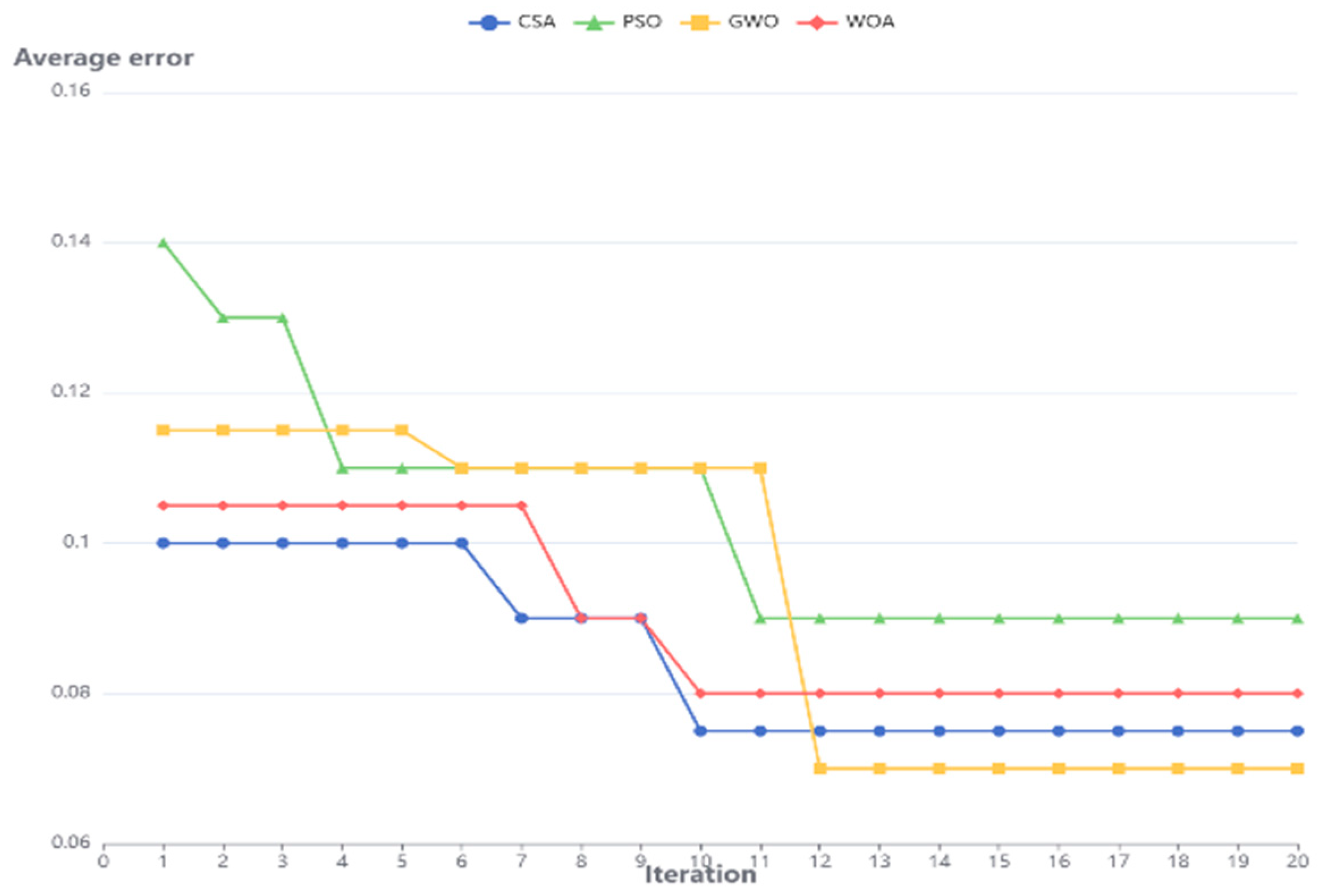
Existing optimization algorithms, such as PSO, WOA, and GWO, have certain limitations when dealing with complex high-dimensional optimization problems. For example, PSO converges quickly in the early stage, but is prone to fall into local optimality in the later stage; although WOA has strong global search capabilities, its optimization efficiency is low. In contrast, the Comprehensive Search Algorithm (CSA) combines the global search capability of MBH and the local optimization capability of SQP, which can effectively improve the convergence speed and accuracy of model parameter optimization. The experimental results show that the IAM-BiLSTM model optimized by CSA is superior to other optimization methods in terms of convergence speed (see Figure 7). As can be seen from the figure, the fitness value of the IAM-BiLSTM model is optimized by the four algorithms, that is, the overall average error shows a downward trend. However, compared with GWO, PSO, and WOA, CSA achieves a shorter average convergence time and the smallest average error. In addition, the error convergence curve obtained by CSA is smoother, and it can be concluded that CSA exhibits better stability and convergence. Therefore, this paper selects CSA as the optimizer of the IAM-BiLSTM model to improve the reliability and generalization ability of the prediction model.

Figure 7. Average Error Convergence Curve.

3.5. Performance Analysis and Evaluation of CSA Optimized IAM-BiLSTM Prediction Model

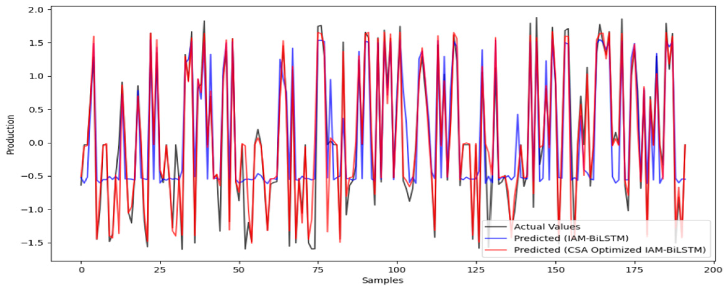
To further validate the optimization capability of CSA for the IAM-BiLSTM prediction model, the CSA-optimized IAM-BiLSTM prediction model was established using the aforementioned production historical data as the dataset. CSA was utilized to optimize the learning rate and feature dimensions of the IAM-BiLSTM prediction model, with specific parameters shown in Table 10. The prediction results are illustrated in Figure 8, and the prediction accuracy comparison results are presented in Table 11. As shown in Table 11, the MAE and MSE of the CSA-optimized IAM-BiLSTM prediction model are 0.0795 and 0.0123, respectively. Compared to IAM-BiLSTM, prediction accuracy has been improved. It can be concluded that optimizing the learning rate, batch size, and the number of neurons in the IAM-BiLSTM prediction model using CSA can effectively enhance the model’s prediction accuracy.

Table 10. Parameter Settings of IAM-BiLSTM Prediction Model Optimized by CSA.

Symbol	Meaning	Value
$R_x$	Maximum rejection times	20
N	Random perturbation amplitude	10%
$L_b$	Optimization range lower limit	[0.001, 1, 1]
$U_b$	Optimization range upper limit	[0.01, 512, 512]

Figure 8. Comparison of Prediction Results of IAM-BiLSTM Optimized by CSA.

Table 11. Comparison of Prediction Accuracy.

Prediction Methods	Meaning	Value
CSA Optimized IAM-BiLSTM	0.0123	0.0795
CSA Optimized IAM-BiLSTM	0.0385	0.1561

4. Results and Conclusions

The high-precision performance of the CSA-optimized IAM-BiLSTM model proposed in this study in oil well production prediction makes it of significant value in oilfield management and commercial applications. First, the model can help oilfield managers optimize production plans, reduce unnecessary equipment maintenance, and improve resource utilization, thereby reducing operating costs. Second, accurate prediction capabilities can help reduce production fluctuations and improve economic benefits. For example, reducing prediction errors can effectively reduce the production capacity loss of oil fields due to misjudgment. Finally, the high efficiency of the model can also reduce energy waste in oilfield production, optimize carbon emission management, and meet the requirements of sustainable development. Therefore, this study not only provides an innovative prediction method at the technical level, but also provides an important reference for intelligent production in the oil and gas industry.

This study validated the IAM-BiLSTM model using a dataset constructed from oilfield production data and compared the prediction performance with various baseline models. By applying multiple optimization algorithms to the parameter optimization of the IAM-BiLSTM model, the following conclusions were drawn:

• A BiLSTM model based on the Inter-Attention Mechanism (IAM-BiLSTM) was proposed, which assigns different weights to hidden states, enhancing the influence of critical information. Experimental results show that the IAM-BiLSTM model outperforms traditional BiLSTM and AM-BiLSTM models in prediction accuracy.
• Compared with optimization algorithms such as GWO, PSO, and WOA, the CSA-optimized IAM-BiLSTM model achieves faster and more stable convergence of its error iteration curve. Experimental results demonstrate that the CSA algorithm has excellent stability and convergence properties, improving the prediction accuracy of the IAM-BiLSTM model.
• The proposed CSA-optimized IAM-BiLSTM model has been successfully applied to production prediction at a specific oil well site in Sichuan, verifying the method’s robustness and generalization ability.