A Transient Control Strategy for Grid-Forming Photovoltaic Systems Based on Dynamic Virtual Impedance and RBF Neural Networks

Abstract

This paper proposes a grid-forming (GFM) photovoltaic system transient control strategy based on the combination of dynamic virtual impedance and the radial basis function (RBF) algorithm. First, the virtual synchronous generator (VSG) model is analyzed to understand how virtual impedance affects current surges and system stability during faults. By using dynamic virtual impedance throughout the fault, the strategy suppresses current spikes and improves stability. The RBF neural network dynamically adjusts virtual inertia and damping coefficients to optimize transient power-angle characteristics and speed up recovery during fault restoration. Simulation results show that the strategy reduces transient current surges, improves angle recovery, and boosts system stability during voltage sag. This approach offers an effective solution for low-voltage ride-through (LVRT) and transient control in photovoltaic grid-connected systems, ensuring the resilience and stability of renewable energy integration into the grid.

1. Introduction

As the penetration of renewable energy in global power systems continues to increase, particularly with the large-scale integration of intermittent sources such as wind and photovoltaic (PV) power, the stability and reliability of power systems are facing significant challenges [1,2,3]. The intermittency and volatility of renewable energy sources require the grid to have higher flexibility and fast response capabilities to address the impact of generation fluctuations on frequency and voltage. Additionally, the increased coupling of the system means that local faults may trigger chain reactions throughout the grid. These factors pose growing challenges to the stability and reliability of modern power systems. Therefore, enhancing the grid’s flexibility and emergency response capabilities, along with adopting new control strategies, is key to addressing these issues. Currently, grid-following (GFL) control is commonly used in grid-connected photovoltaic systems. Researchers have focused on low-voltage ride-through (LVRT) control during grid faults. For instance, Reference [4] derived the voltage magnitude at the grid connection point under unbalanced faults based on the output characteristics of inverters during these faults and used inverter output current thresholds to determine the optimal reactive current at different voltage sag stages, achieving voltage support. Reference [5] adjusted PV output power based on the depth of the grid-side voltage sag to maintain a constant DC bus voltage, but the control structure employed GFL control without energy storage devices for power smoothing, leading to inadequate transient control performance. Reference [6] used a DC bus overvoltage ring control to maintain a constant DC bus voltage, but the DC bus voltage increases during LVRT. References [7,8] studied the regulation of adaptive energy management under abnormal photovoltaic operation conditions, utilizing energy storage systems and other methods. By considering the dynamic characteristics of the energy storage system, control algorithms were employed to effectively enhance the voltage sustainability of the DC microgrid, providing strong evidence for the feasibility of the energy storage system.

To improve the stability of power systems under large-scale PV integration, grid-forming (GFM) control, such as virtual synchronous generator (VSG) technology, has the ability to actively regulate the frequency and voltage of the power grid, meaning it can maintain the stability of the system’s frequency and voltage even without an external grid. Additionally, when the grid experiences large-scale faults, the GFM control can simulate the inertia of synchronous generators, providing support similar to mechanical inertia. This virtual inertia effectively dampens instantaneous frequency fluctuations and helps the system quickly recover when disturbances occur. Compared to traditional GFL control that rely on the frequency and voltage of the external grid, GFM can better withstand transient disturbances in the grid and reduce the risk of large-scale instability [9,10]. Furthermore, to prevent power interruptions during faults and ensure continuous supply to critical loads, existing research has focused on PV derating or the use of energy storage systems. However, PV derating alone cannot provide sufficient power support to the grid and has limited regulation capabilities. The use of energy storage devices can effectively address the dynamic stability challenges faced by power systems after renewable energy integration [11], the charging and discharging mechanisms of the energy storage system have a significant impact on virtual inertia and damping coefficients. During a fault, when the energy storage system discharges, it can provide rapid power support, enhancing virtual inertia and improving the damping effect, thereby increasing the stability of the grid. On the other hand, during charging, the response of the energy storage system to frequency fluctuations is weaker, which may result in poorer system damping.

Domestic and international scholars have conducted a series of studies on the transient control of VSG under grid voltage faults. There are two main current-limiting strategies during faults. One approach switches control strategies during faults. Reference [12] directly controls current during faults but fails to fully utilize the stability and fault response capabilities provided by VSG control, particularly in terms of fast grid frequency recovery, current impact limitation, and dynamic recovery performance. Reference [13] switches the PV inverter’s VSG control to model predictive control (MPC) after a ground fault occurs and switches back to VSG control after fault clearing, but the control strategy during faults is complex. Another approach modifies the control loop for integrated current limiting. Reference [14] proposed a dynamic current-limiting control strategy based on virtual impedance and power limitations but did not analyze the impact of virtual impedance values under different fault severities. References [15,16,17] proposed a series of integrated current-limiting measures but lacked a comprehensive analysis of transient power-angle characteristics during faults. Reference [18] analyzed the transient power-angle characteristics and current-limiting control, effectively suppressing short-circuit currents while ensuring stability, but lacked an analysis of the coupling relationships between control parameters.

Therefore, domestic and international scholars have conducted extensive research on the adjustment of VSG parameters. Reference [19] proposed an adaptive adjustment of VSG virtual inertia using the bang–bang algorithm, but during the adjustment process, there was a lack of analysis of the damping coefficient, and abrupt parameter changes could destabilize the system. References [20,21] analyzed the impact of VSG control parameters on small disturbance stability using a dual-stage PV system, but small signal modeling methods are not applicable during faults, and transient characteristics were not analyzed. Reference [22] performed adaptive adjustment of virtual inertia and damping coefficients but only qualitatively controlled them based on angular frequency and its change rate, without discussing the angle control characteristics, leading to lower control accuracy. Reference [23] used the radial basis function (RBF) algorithm for adaptive adjustment of virtual inertia to improve control accuracy, but the transient characteristics of VSG during faults and recovery were not discussed. From the above analysis, it is evident that existing control strategies do not fully consider the impact of control parameters throughout the entire fault process on transient power-angle characteristics and lack dynamic current-limiting measures and adaptability during different voltage sag levels and fault recovery stages.

Table 1. Existing control strategies.

Control Strategies	Advantages	Disadvantages
Switching control strategies (MPC) during faults	Based on real-time changes in the grid state, MPC can dynamically adjust control inputs, making it highly optimized and adaptable.	The control strategy is complex, and the switching process may introduce control instability.
Dynamic current-limiting control	Uses virtual impedance and power limitations for current limiting.	No analysis of virtual impedance effects under different fault severities.
Adaptive adjustment of virtual inertia (bang–bang algorithm)	The algorithm is excellent and adapts to adjust virtual inertia.	Lacks analysis of damping coefficients, abrupt parameter changes destabilize the system.
RBF algorithm for adaptive adjustment	The RBF algorithm provides more precise adaptive control of virtual inertia and can effectively handle nonlinear systems, adapting to the complex changes in grid conditions.	Lacks discussion of VSG’s transient characteristics during faults.

summarizes the pros and cons of current VSG control strategies.

The core objective of the LVRT control strategy is to ensure that the system remains stable during voltage sags, preventing inverter disconnection due to voltage sags and thus avoiding system interruptions. Therefore, to further investigate and optimize the control strategy, this paper proposes a transient control strategy for GFM photovoltaic systems based on dynamic virtual impedance and RBF neural networks. This strategy, considering the fault process characteristics, allows the system’s virtual inertia and damping coefficient to adaptively adjust according to the angular velocity variation, while also incorporating fault current-limiting measures. First, the mathematical model and basic principles of the PV-storage grid-connected virtual synchronous generator (VSG) are analyzed. Secondly, using the equal-area criterion and a power command adjustment strategy based on voltage sag, the impact of virtual impedance on current surges and stability during faults is comprehensively analyzed, considering inverter current constraints. Dynamic virtual impedance is applied to reduce current surges throughout the fault process, while the flexible adjustment capabilities of RBF neural network parameters allow the VSG to dynamically adjust its characteristics more flexibly during fault recovery, optimizing the stability of the power system. Finally, simulation results show that the proposed dual-control strategy not only improves the LVRT capability but also significantly enhances the system stability during the fault recovery process.

2. The GFM Photovoltaic System Model

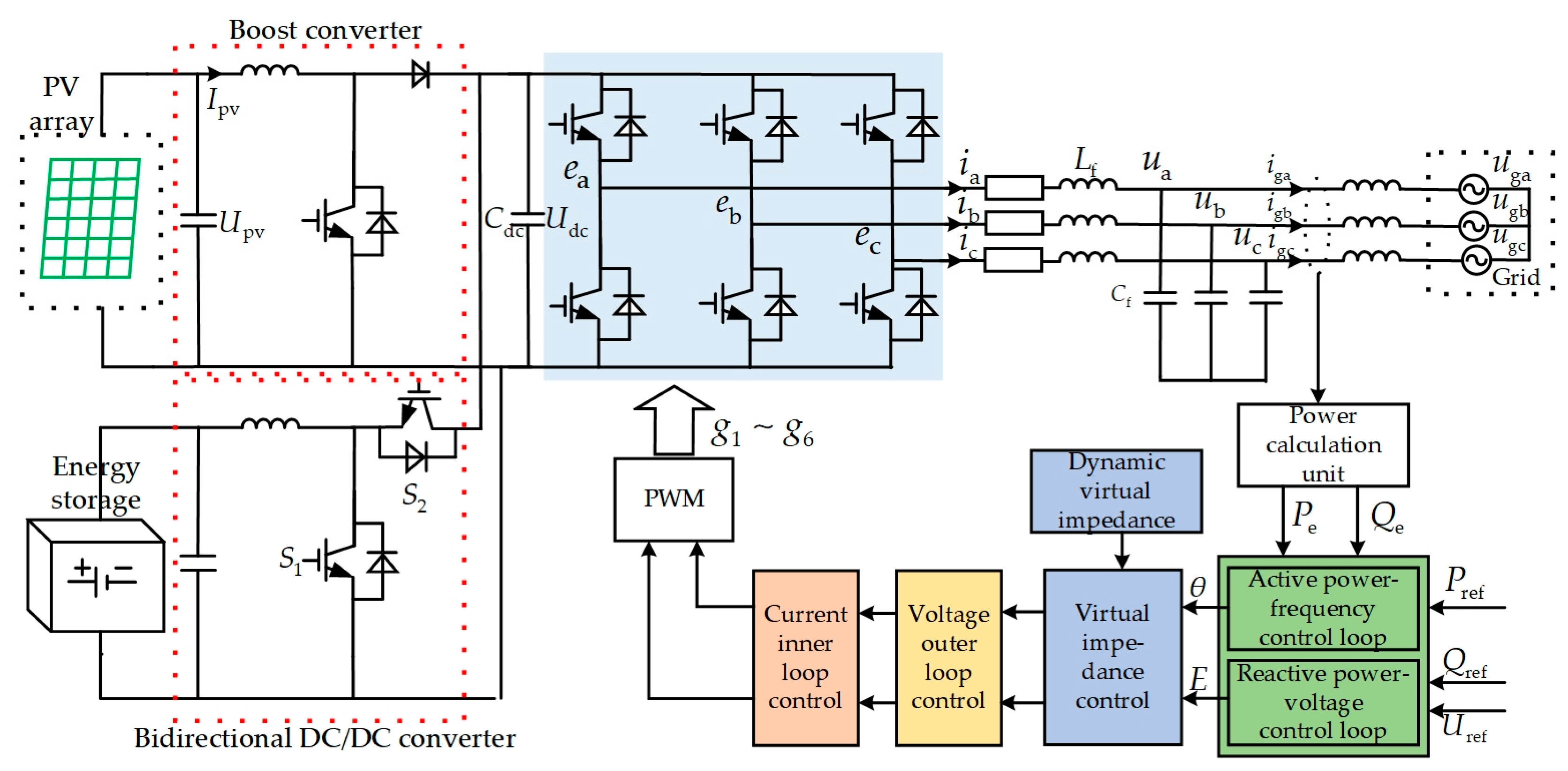
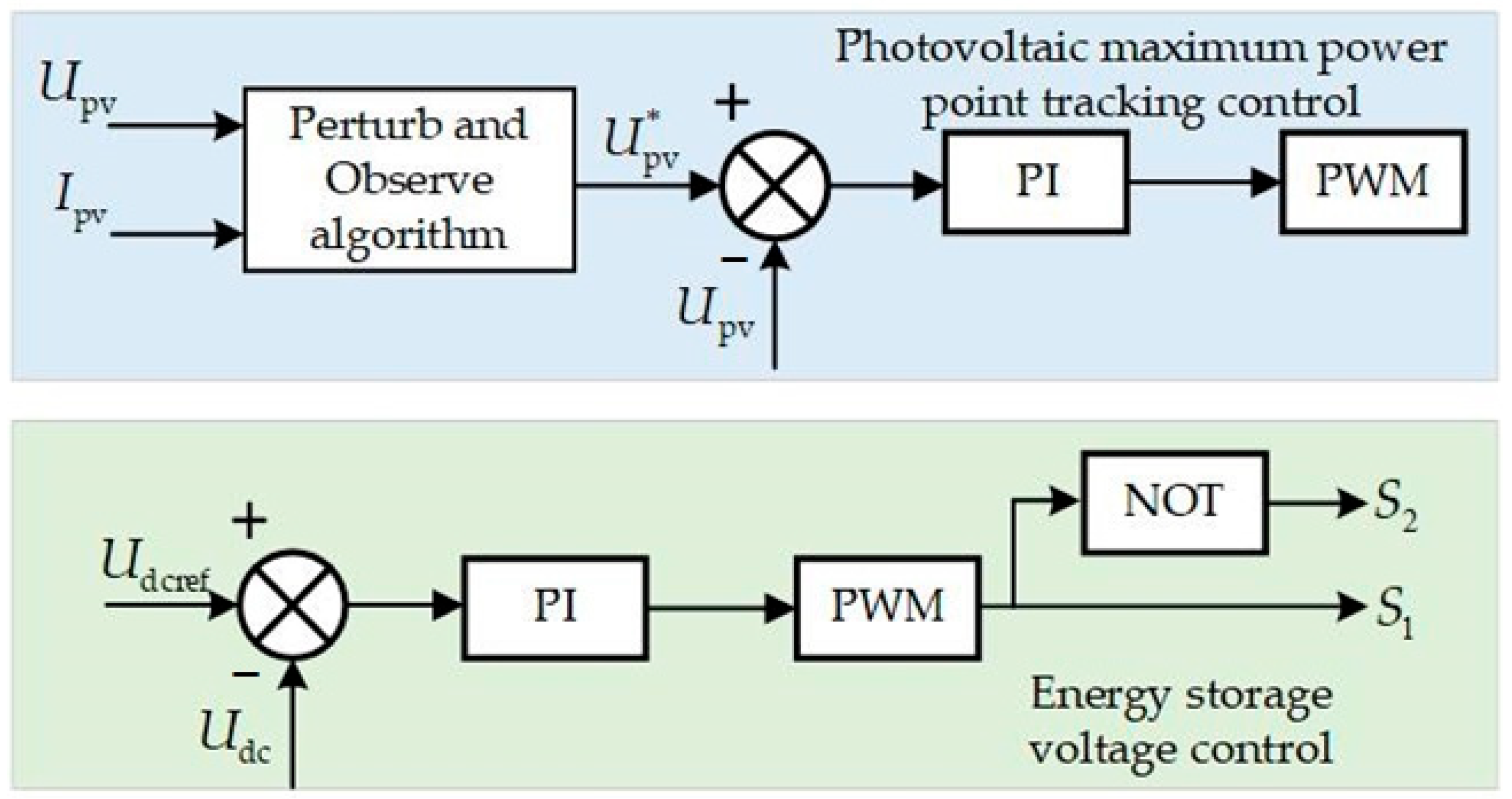
2.1. Topology of the Grid-Forming Photovoltaic System

A GFM photovoltaic system mainly consists of four components: the photovoltaic array, the energy storage system, the three-phase two-level grid-connected inverter, and the AC grid. The VSG control of the photovoltaic inverter imitates the external characteristics of a SG, enabling the photovoltaic system to possess virtual inertia and virtual damping, thus providing frequency and voltage regulation functions. This allows for grid-friendly integration of the photovoltaic system, with energy storage configured on its DC side to stabilize the DC bus voltage. The main circuit topology and control system of the GFM photovoltaic system are shown in Figure 1. In the figure: $C_{\mathrm{dc}}$ represents the DC-side capacitor; $L_{\mathrm{f}}$ and $C_{\mathrm{f}}$ are the filter inductance and filter capacitance, respectively; $e_{\mathrm{abc}}$ is the virtual internal voltage of the inverter; $u_{\mathrm{abc}}$ is the three-phase voltage at the grid connection point; $u_{\mathrm{gabc}}$ is the grid-side voltage; $i_{\mathrm{abc}}$ is the three-phase output current of the inverter; and $i_{\mathrm{gabc}}$ is the three-phase current at the grid connection.

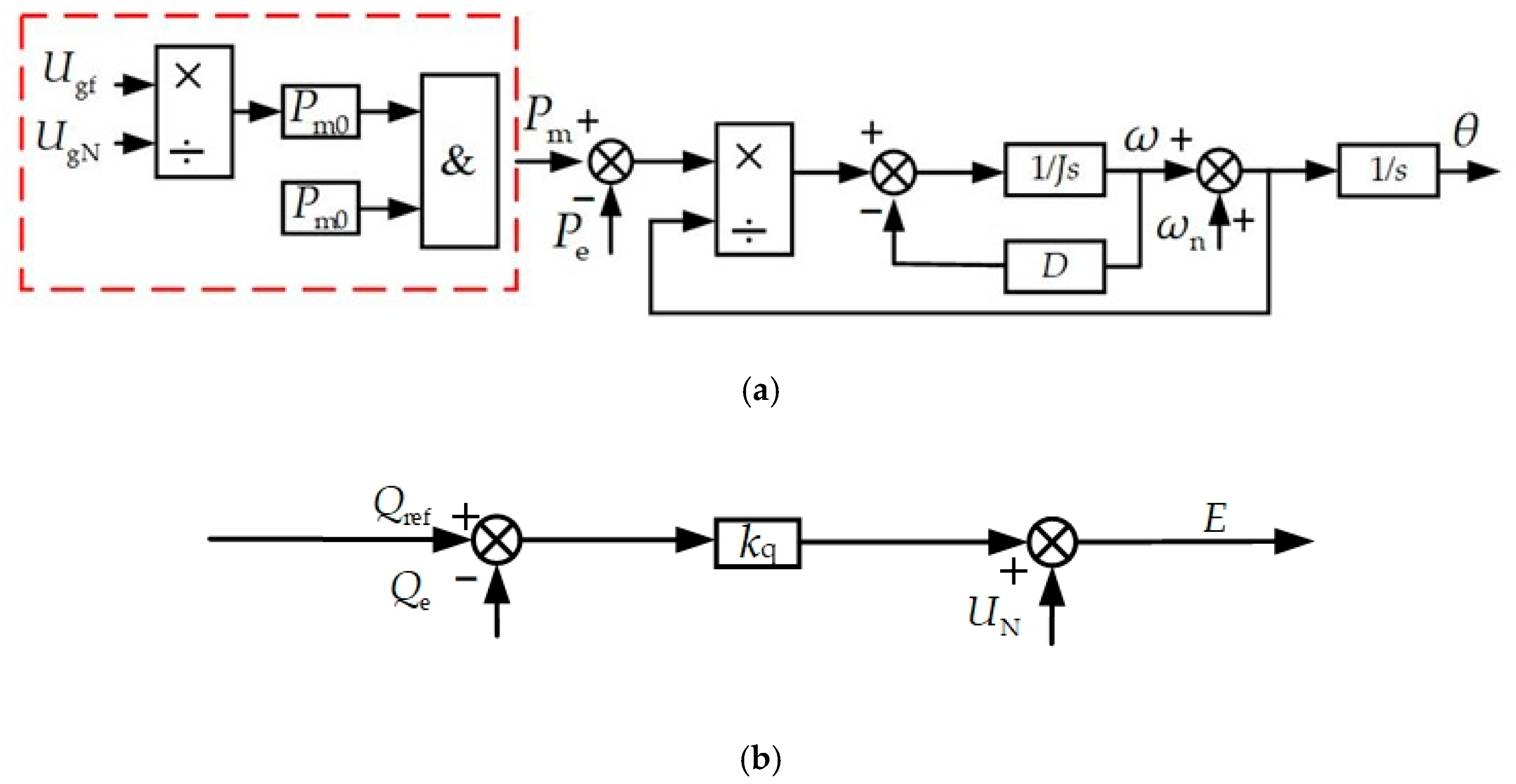
2.2. The Control Strategy

The photovoltaic and energy storage VSG technology integrates the advantages of photovoltaic power generation and energy storage systems, enhancing the dynamic response capability of the PV-storage grid-connected system [24]. In this system, the photovoltaic array output voltage is raised to an appropriate voltage level using a boost converter, the P&O algorithm [25] is employed for maximum power point tracking (MPPT) to control the output active power, and by using the PI controller to compare the actual voltage $U_{\mathrm{pv}}$ with the ideal voltage $U_{\mathrm{pv}}^{*}$. For the voltage control of the energy storage system, a voltage closed-loop control method is employed to stabilize the DC voltage at the storage port, with the State of Charge (SOC) introduced as a key constraint. The SOC value is updated in real-time based on the charging and discharging conditions of the energy storage system. During transient events, the energy availability of the storage system is dynamically adjusted according to changes in SOC, as well as the magnitude and frequency of voltage fluctuations, ensuring system stability and continuous energy supply. If SOC exceeds the set threshold, the system may become unstable, requiring additional protective measures. Specifically, when photovoltaic power is excessive, the energy storage system absorbs the surplus power; when photovoltaic power is insufficient, the energy storage system releases energy to meet the converter’s power demand. The combination of these two control strategies ensures that the converter maintains DC-side voltage stability during grid connection and enables automatic power adjustment. The control block diagram is shown in Figure 2. The active power equation for the grid is presented in Equation (1).

$$P_{\mathrm{pv}}+P_{\mathrm{ess}}=P_{\mathrm{loss}}+P_{\mathrm{inv}}$$

(1)

where $P_{\mathrm{pv}}, P_{\mathrm{ESS}}, P_{\mathrm{loss}}$ and $P_{\mathrm{inv}}$ represent the active power output from the photovoltaic array, the active power output from the energy storage system, the active power loss, and the active power output from the inverter to the grid, respectively.

The VSG control technology, based on conventional converter control strategies, introduces the dynamic characteristics equation of the synchronous generator. This simulates the active power frequency regulation and reactive power voltage regulation from the external characteristics of a synchronous machine, enabling the converter to provide inertia and droop characteristics that support system frequency and voltage fluctuations [26]. In the active power–frequency loop of Figure 1, the rotor mechanical equation is introduced based on the virtual speed governor droop control, incorporating virtual inertia $J$ and damping coefficient $D$. By adjusting the power, it achieves virtual mechanical torque output control. The introduction of virtual inertia allows the VSG to have inertia in active power regulation, while the damping coefficient is introduced to suppress power oscillations during the power regulation process. The rotor mechanical equation is shown in Equation (2).

$$\left\{\begin{array}{l}J{\displaystyle \frac{{\mathrm{d}}^2\mathsf{\delta }}{\mathrm{d}{t}^2}}=T_{\mathrm{m}}-T_{\mathrm{e}}-T_{\mathrm{d}}\\ T_{\mathrm{m}}={\displaystyle \frac{P_{\mathrm{m}}}{\omega }},T_{\mathrm{e}}={\displaystyle \frac{P_{\mathrm{e}}}{\omega }},T_{\mathrm{d}}=D{\displaystyle \frac{\mathrm{d}\mathsf{\delta }}{\mathrm{d}t}}\\ \mathsf{\delta }={\displaystyle \int (\omega -{\omega }_{\mathrm{n}})\mathrm{d}t}\end{array}\right.$$

(2)

where $\mathsf{\delta }, \omega$ and ${\omega }_{\mathrm{n}}$ represent the power angle, angular velocity, and rated angular velocity of the VSG, respectively; $T_{\mathrm{m}}, T_{\mathrm{e}}$ and $T_{\mathrm{d}}$ represent the mechanical torque, electromagnetic torque, and damping torque, respectively; $P_{\mathrm{m}}$ and $P_{\mathrm{e}}$ represent the mechanical power and electromagnetic power, respectively; $J$ and $D$ represent the virtual inertia and damping coefficient of the VSG, respectively.

The VSG not only has an active power–frequency control loop that simulates the frequency regulation characteristics of a synchronous generator, but it also has excitation regulation characteristics. Similarly, it can simulate the excitation current control method of a SG to achieve voltage amplitude regulation. In the reactive power–voltage control loop of Figure 1, by analogy with the rotor mechanical equation, the reactive power–voltage regulation equation can be derived as:

$$E=U_{\mathrm{N}}+k_{\mathrm{q}}(Q_{\mathrm{ref}}-Q_{\mathrm{e}})$$

(3)

where $E$ and $U_{\mathrm{N}}$ represent the reference output voltage and the rated voltage of the VSG, respectively; $Q_{\mathrm{ref}}$ and $Q_{\mathrm{e}}$ represent the commanded reactive power and the actual reactive power output of the VSG, respectively; $k_{\mathrm{q}}$ represents the reactive power droop coefficient.

3. The GFM Photovoltaic LVRT Control Strategy

The core goal of the LVRT control strategy is to ensure that the system can maintain stable operation during voltage sag, preventing inverter disconnection due to voltage dips, thereby avoiding system interruptions. Therefore, the use of dynamic virtual impedance and an RBF neural network-based dynamic adjustment mechanism enhances the system’s adaptability and robustness, effectively improving the system’s LVRT capability during voltage disturbances, ensuring the stability and reliability of the system.

3.1. Inverter Overcurrent Capability Analysis

The overcurrent capability of an inverter mainly refers to the maximum short-circuit current or instantaneous current peak that the inverter can withstand without damage. The converter’s output current tolerance threshold can reach 1.1 to 2 times the rated current. When the fault current exceeds the converter’s tolerance, it will lead to damage to the converter and affect the stability of the power system [27]. When a fault occurs, causing a voltage sag, the voltage magnitude and phase of the VSG should not experience abrupt changes. Therefore, the output current of the VSG during the fault period is:

$$I_{\mathrm{f}}(t)=I_{\mathrm{k}}(t)+(I_{\mathrm{f}0}-I_{\mathrm{k}0})e^{-{\displaystyle \frac{R_{\mathrm{f}}}{L_{\mathrm{f}}}}t}$$

(4)

where $I_{\mathrm{k}}(t)$ represents the steady-state value of the short-circuit current after the grid voltage sag; $I_{\mathrm{f}0}$ represents the instantaneous output current of the VSG before the grid voltage sag; $I_{\mathrm{k}0}$ represents the initial value of the periodic component of the short-circuit current after the grid voltage sag; $R_{\mathrm{f}}$ and $L_{\mathrm{f}}$ represent the resistance and inductance of the VSG and the grid side after the grid voltage sag, respectively.

Define the grid voltage phasor as the reference, then the instantaneous output current of the VSG before the grid voltage sag is:

$$I_{\mathrm{f}0}={\displaystyle \frac{U_{\mathrm{o}0}\angle {\mathsf{\delta }}_0-U_{\mathrm{g}0}\angle 0}{\mathrm{j}{Z}_0}}$$

(5)

where $U_{\mathrm{o}0}$ and $U_{\mathrm{g}0}$ represent the actual output voltage of the VSG and the grid-side voltage, respectively, before the grid voltage sag; ${\mathsf{\delta }}_0$ represents the phase difference between the actual output voltage phasor of the VSG and the grid voltage phasor before the grid voltage sag; $Z_0$ represents the equivalent impedance between the VSG and the grid-side before the grid voltage sag.

The instantaneous output current of the VSG after the grid voltage sag is:

$$I_{\mathrm{k}}={\displaystyle \frac{U_{\mathrm{of}}\angle {\mathsf{\delta }}_{\mathrm{f}}-U_{\mathrm{gf}}\angle 0}{\mathrm{j}{Z}_{\mathrm{f}}}}$$

(6)

where $U_{\mathrm{of}}$ and $U_{\mathrm{gf}}$ represent the actual output voltage of the VSG and the grid-side voltage, respectively, after the grid voltage sag; ${\mathsf{\delta }}_{\mathrm{f}}$ represents the phase difference between the actual output voltage phasor of the VSG and the grid voltage phasor after the grid voltage sag; $Z_{\mathrm{f}}$ represents the equivalent impedance between the VSG and the grid-side after the grid voltage sag.

Thus, when a fault occurs in the grid causing a voltage sag, the VSG will output a relatively large short-circuit current. The magnitude of this short-circuit current is mainly related to the depth of the voltage sag, the equivalent impedance between the VSG and the grid side, and the phase difference. Therefore, to prevent the switching devices from being damaged by prolonged overcurrent and to ensure the safe and stable operation of the system, appropriate current-limiting control strategies must be implemented.

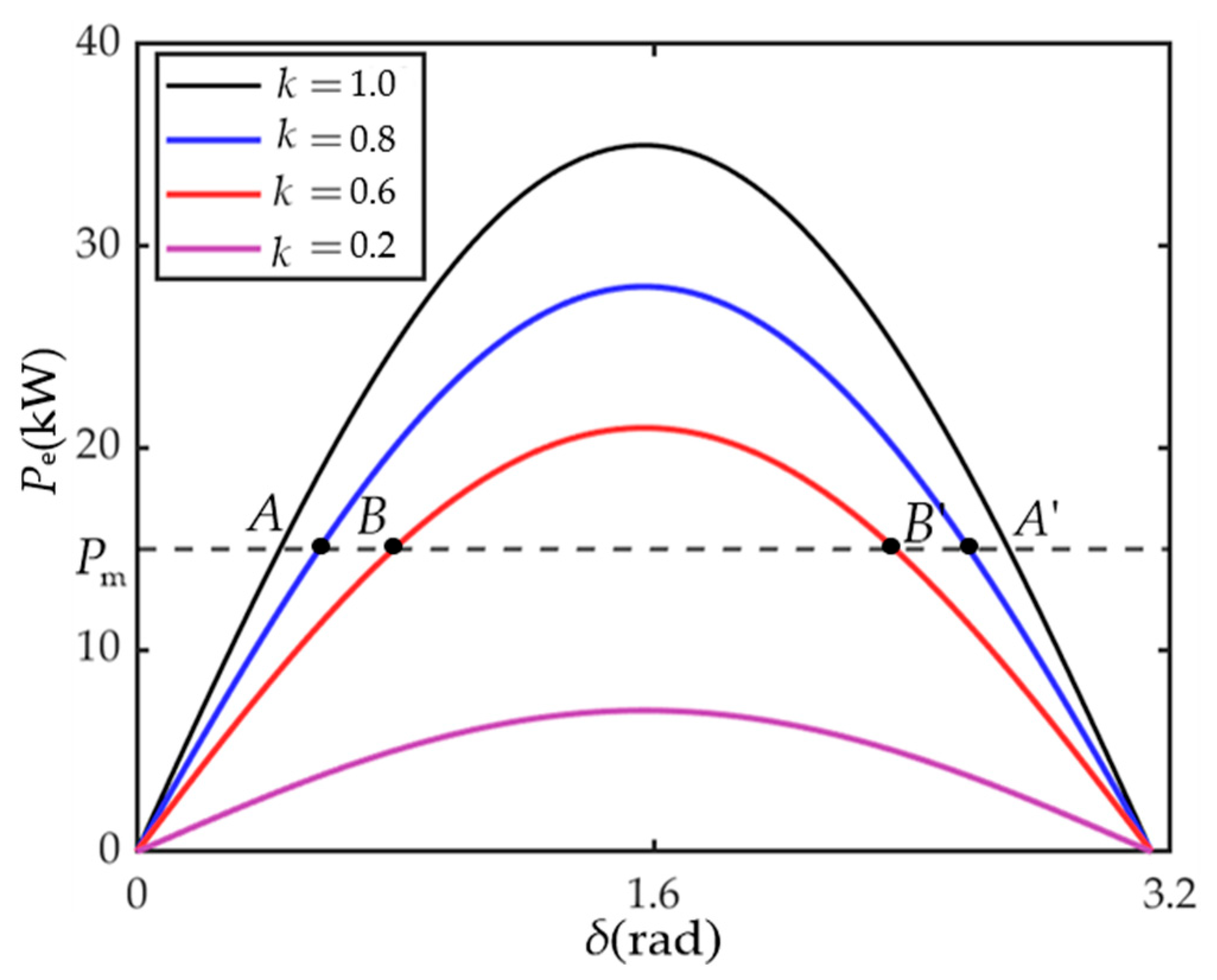
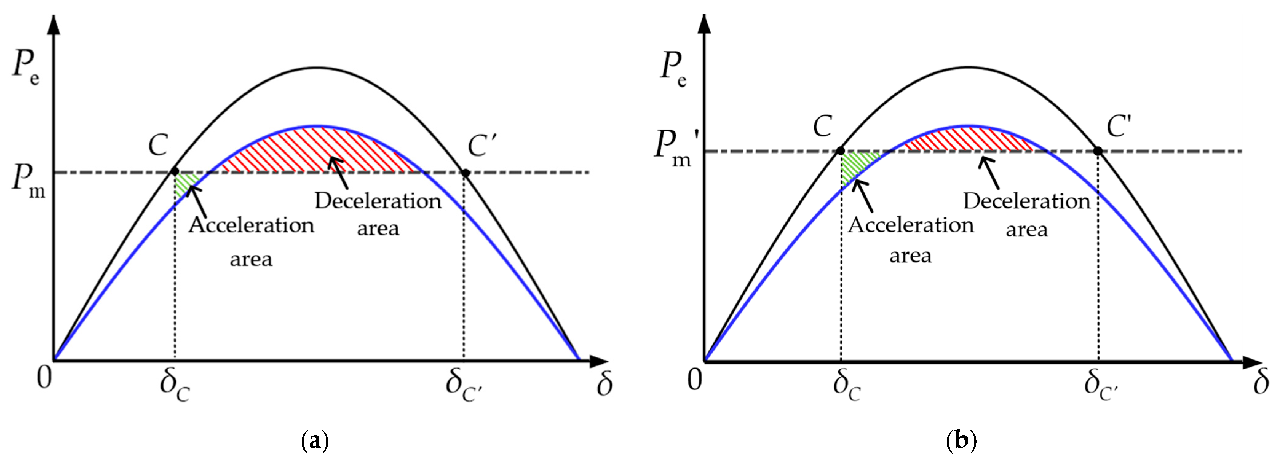
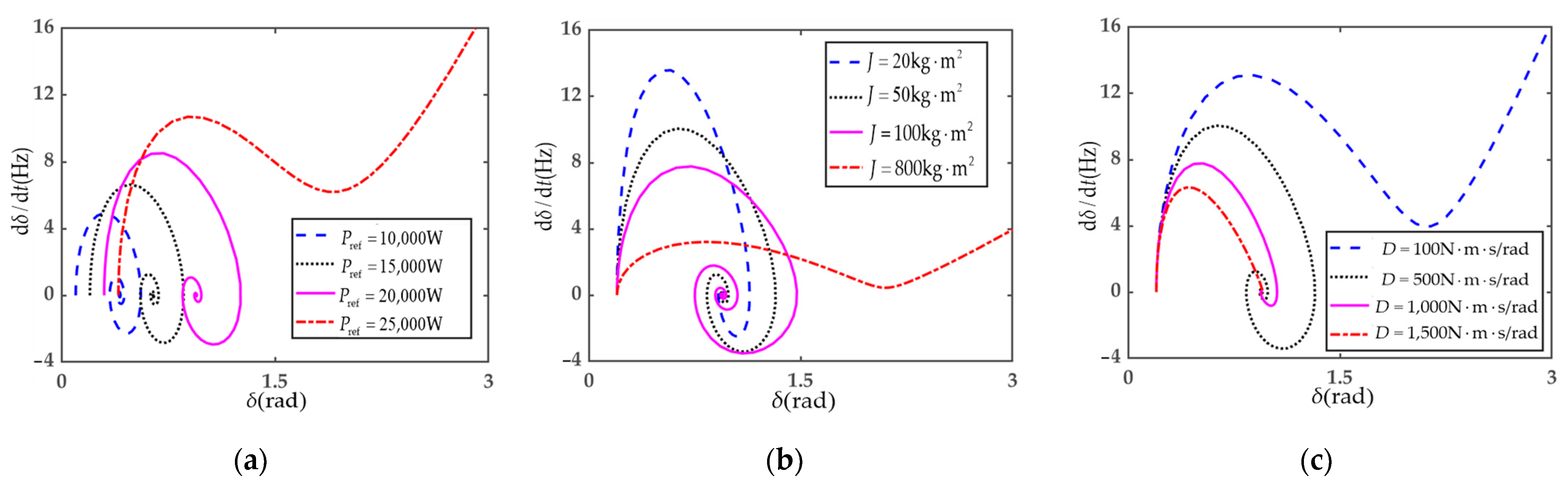
3.2. Power-Angle Stability Analysis

Since the distance between the converter and the grid is generally quite long, the line resistance is typically neglected, i.e., $X_{\mathrm{g}}>>R_{\mathrm{g}}$. Therefore, the line impedance can be approximated as purely inductive. In this case, the active and reactive power transmitted between the VSG and the grid are:

$$\left\{\begin{array}{l}{P}_{\mathrm{e}}={\displaystyle \frac{3E{U}_{\mathrm{g}}}{2X_{\mathrm{g}}}}\sin \mathsf{\delta }\\ Q_{\mathrm{e}}={\displaystyle \frac{3E^2-3E{U}_{\mathrm{g}}\cos \mathsf{\delta }}{2X_{\mathrm{g}}}}\end{array}\right.$$

(7)

Considering the influence of the VSG’s reactive power loop, substituting the reactive power equation from Equation (7) into Equation (3) yields the following quadratic equation in terms of $E$:

$$1.5k_{\mathrm{q}}{E}^2+(X_{\mathrm{g}}-1.5k_{\mathrm{q}}{U}_{\mathrm{g}}\cos \mathsf{\delta })E-\left(U_{\mathrm{N}}+k_{\mathrm{q}}{Q}_{\mathrm{ref}}\right)X_{\mathrm{g}}=0$$

(8)

Solving the quadratic equation yields:

$$E={\displaystyle \frac{1.5k_{\mathrm{q}}{U}_{\mathrm{g}}\cos \mathsf{\delta }-X_{\mathrm{g}}+\sqrt{{(X_{\mathrm{g}}-1.5k_{\mathrm{q}}{U}_{\mathrm{g}}\cos \mathsf{\delta })}^2+6k_{\mathrm{q}}{X}_{\mathrm{g}}(U_{\mathrm{N}}+k_{\mathrm{q}}{Q}_{\mathrm{ref}})}}{3k_{\mathrm{q}}}}$$

(9)

Considering the effect of the reactive power loop, substituting the active power equation from Equation (9) and the reactive power equation from Equation (7) into Equation (2) gives:

$$\begin{array}{l}J{\omega }_{\mathrm{n}}{\displaystyle \frac{{\mathrm{d}}^2\delta }{\mathrm{d}{t}^2}}+D{\omega }_{\mathrm{n}}{\displaystyle \frac{{\mathrm{d}}^2\delta }{\mathrm{d}{t}^2}}=P_{\mathrm{m}}-{\displaystyle \frac{3U_{\mathrm{g}}^2}{8X_{\mathrm{g}}}}\sin 2\mathsf{\delta }+{\displaystyle \frac{U_{\mathrm{g}}\sin \mathsf{\delta }}{2k_{\mathrm{q}}}}\\ -{\displaystyle \frac{U_{\mathrm{g}}\sqrt{{(X_{\mathrm{g}}-1.5k_{\mathrm{q}}{U}_{\mathrm{g}}\cos \mathsf{\delta })}^2+6k_{\mathrm{q}}{X}_{\mathrm{g}}(U_{\mathrm{N}}+k_{\mathrm{q}}{Q}_{\mathrm{ref}})}}{2k_{\mathrm{q}}{X}_{\mathrm{g}}}}\sin \mathsf{\delta }\end{array}$$

(10)

Let the state variable be $x={\left[x_1,x_2\right]}^T={\left[\mathsf{\delta },{\displaystyle \frac{\mathrm{d}\mathsf{\delta }}{\mathrm{d}t}}\right]}^T$. Since the bandwidth of the VSG voltage–current inner loop is much larger than that of the VSG power loop, the dynamic characteristics of the voltage–current inner loop can be ignored. Therefore, the reduced-order state-space model or large-signal model of the VSG is:

$$\left[\begin{array}{l}\stackrel{•}{x_1}\\ \stackrel{•}{x_2}\end{array}\right]=\left[\begin{array}{l}{x}_2\\ {\displaystyle \frac{P_{\mathrm{m}}}{J{\omega }_{\mathrm{n}}}}-{\displaystyle \frac{3E{U}_{\mathrm{g}}}{2J{\omega }_{\mathrm{n}}{X}_{\mathrm{g}}}}\sin \mathsf{\delta }-{\displaystyle \frac{D{x}_2}{J{\omega }_{\mathrm{n}}}}\end{array}\right]$$

(11)

Therefore, define $k$ as the ratio of the fault voltage to the grid voltage. Under the influence of the reactive power loop, the power-angle curves of the VSG for different fault severities and different active power command values are shown in Figure 3 and Figure 4.

In Figure 3, for voltage sags of 20% and 40%, the power-angle curve of the VSG intersects with the mechanical power $P_{\mathrm{m}}$, while for a voltage sag of 80%, the power-angle curve no longer intersects with $P_{\mathrm{m}}$. If the system intersects $P_{\mathrm{m}}$ at points A and B during the fault, it is considered to be at a stable equilibrium point (SEP); if the system intersects $P_{\mathrm{m}}$ at points A’ and B’, it is considered to be at an unstable equilibrium point (UEP), which could lead to transient instability.

According to the equal-area criterion of power system transient stability [28], the condition for the system to maintain transient stability is that the maximum accelerating area should be less than the maximum decelerating area. From Figure 4, it can be seen that the standard power-angle curve is shown in black, and after a voltage drop occurs, it is shown in blue. As the active power command value increases, the accelerating area increases while the decelerating area decreases. Therefore, an increase in the active power command value will affect the transient stability characteristics of the VSG and may even lead to instability.

Thus, in this paper, based on the grid voltage sag degree and combined with Equations (2), (3) and (7), the active power loop adopts a VSG grid voltage response-based power dispatch strategy. According to the relevant provisions of reference [29], reactive power is increased by issuing additional reactive power. The power loop control block diagram is shown in Figure 5, where the reactive current injected by the inverter into the grid, $I_{\mathrm{dref}}$ and $I_{\mathrm{qref}}$, must satisfy:

$$\left\{\begin{array}{l}{I}_{\mathrm{dref}}=\sqrt{I_{\mathrm{N}}^2-I_{\mathrm{qref}}^2},I_{\mathrm{N}}^2-I_{\mathrm{qref}}^2>0.9\\ I_{\mathrm{dref}}=0,I_{\mathrm{N}}^2-I_{\mathrm{qref}}^2<0\end{array}\right.$$

(12)

$$\left\{\begin{array}{l}{I}_{\mathrm{qref}}=0,{\displaystyle \frac{U_{\mathrm{gf}}}{U_{\mathrm{gN}}}}>0.9\\ I_{\mathrm{qref}}=1.5\times \left(0.9-{\displaystyle \frac{U_{\mathrm{gf}}}{U_{\mathrm{gN}}}}\right)I_{\mathrm{N}},0.2\le {\displaystyle \frac{U_{\mathrm{gf}}}{U_{\mathrm{gN}}}}\le 0.9\\ I_{\mathrm{qref}}=1.5I_{\mathrm{N}},{\displaystyle \frac{U_{\mathrm{gf}}}{U_{\mathrm{gN}}}}<0.2\end{array}\right.$$

(13)

where $I_{\mathrm{N}}$ represents the rated output current of the inverter.

To analyze the impact of different parameters on the transient characteristics of the VSG during a system fault, the phase plane diagrams for different values of $P_{\mathrm{ref}}, J$ and $D$ are plotted during the fault period when a SEP exists, as shown in Figure 6, based on the second-order differential equation in Equation (10).

As shown in Figure 6a, with the increase in active power command value, the initial power angle of the VSG gradually increases, and the system transitions from transient stability to transient instability, which is consistent with the analysis result in Figure 5.

Even if an equilibrium point exists at the moment of the fault, instability may still occur due to incorrect control parameter settings. From Figure 6b,c, it can be seen that when $D$ remains constant, an increase in $J$ will lead to a decrease in system stability. However, an increase in $J$ will slow down the rate of change in the power angle, helping to suppress power-angle overshoot. Conversely, a smaller $J$ is beneficial for maintaining system stability but will lead to a larger rate of change in the power angle, which is unfavorable to the system’s stability during fault recovery. When $J$ remains constant, an increase in $D$ will improve system stability and shorten the corresponding adjustment time, while also slowing down the rate of change in the power angle, helping to suppress power-angle overshoot. When $D$ is small, it will reduce the damping effect on system oscillations, thereby accelerating the system’s response to external disturbances. Therefore, it is necessary to comprehensively consider the dynamic adjustment characteristics of system parameters throughout the fault period, as described later in the dynamic adjustment strategy based on the BRF neural network.

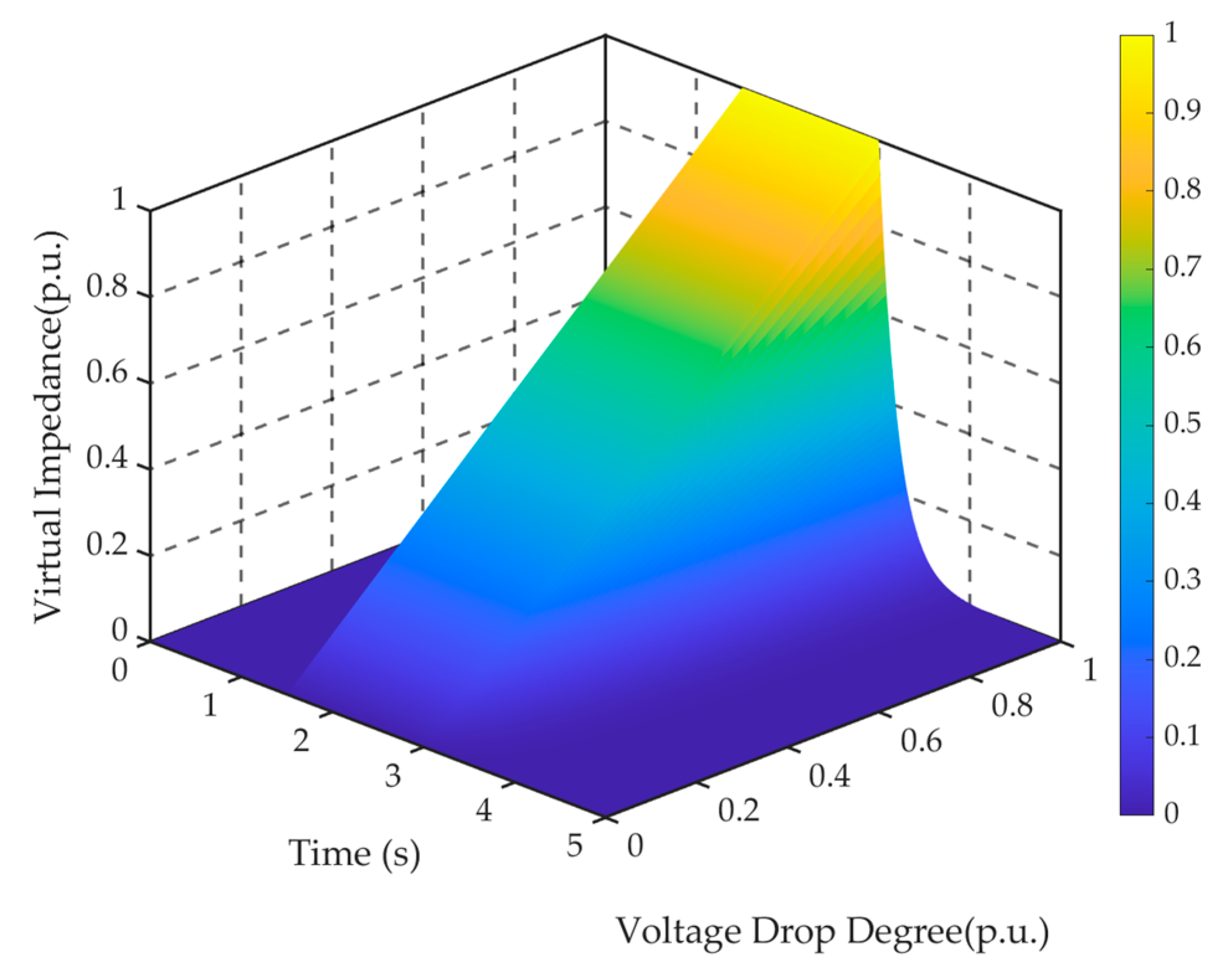
3.3. Dynamic Virtual Impedance Control

During fault occurrence and clearance, the grid voltage undergoes significant instantaneous fluctuations. Due to the response delay in the control system, these fluctuations may lead to large transient current surges and non-periodic components in the grid-connected inverter, further affecting the grid’s stability and power quality [30]. To ensure the stability and reliability of the power system, dynamic virtual impedance plays a crucial role under different fault scenarios. The virtual impedance can be dynamically adjusted based on the severity of the system fault to respond to the real-time conditions of the grid. When the grid voltage is at a higher level, using lower virtual impedance helps ensure that the system can output sufficient power, avoiding unnecessary power loss and efficiency reduction caused by excessive virtual impedance. In this case, lower virtual impedance effectively facilitates power transmission, ensuring that the system can quickly restore normal operation under high voltage conditions.

Conversely, when the grid voltage significantly drops, increasing virtual impedance can effectively limit excessive current flow, thereby reducing the impact of short-circuit currents and preventing equipment damage or triggering protection mechanisms due to high currents. By increasing virtual impedance, the system can restrict current flow, alleviating the system stress caused by short circuits or rapid voltage drops. This mechanism helps maintain grid stability and prevents the detrimental effects of sudden current fluctuations on electrical equipment.

To address these issues, dynamic virtual impedance can be introduced in the grid-connected inverter. By introducing dynamic virtual impedance between the inverter’s internal virtual potential and output voltage, the system can perform real-time adjustments according to the instantaneous voltage fluctuations of the grid. When the grid voltage is higher, the virtual impedance is appropriately reduced to promote smooth power output; while in the event of a sharp voltage drop, the virtual impedance is increased to limit current flow, preventing the power system from encountering overcurrent damage. Additionally, dynamic virtual impedance can accelerate the decay of short-circuit currents, assisting the system in quickly restoring to normal operating conditions, thereby enhancing the overall robustness and responsiveness of the system. The dynamic virtual impedance is shown in Figure 7, the value of $Z_{\mathrm{v}}$ is as shown in Equation (14).

$$Z_{\mathrm{v}}=\left\{\begin{array}{l}0,t\le t_0\\ k(R_{\mathrm{v}}+j{\omega }_{\mathrm{n}}{L}_{\mathrm{v}}),t_0<t\le t_1\\ k(R_{\mathrm{v}}+j{\omega }_{\mathrm{n}}{L}_{\mathrm{v}})e^{-\alpha (t-t_1)},t>t_1\end{array}\right.$$

(14)

where $R_{\mathrm{v}}$ represents virtual resistance; $L_{\mathrm{v}}$ denotes virtual reactance; $t_0$ is the time of fault occurrence; $t_1$ is the time of fault clearance; and $\alpha$ is the virtual impedance decay coefficient.

To dynamically adjust the voltage reference value while neglecting the impact of transient components, the VSG voltage loop control equation considering the introduction of dynamic virtual impedance is given by:

$$\left\{\begin{array}{l}{U}_{\mathrm{dref}}=E_{\mathrm{dref}}-R_{\mathrm{v}}{I}_{\mathrm{d}}+{\omega }_{\mathrm{n}}{L}_{\mathrm{v}}{I}_{\mathrm{q}}\\ U_{\mathrm{qref}}=0-R_{\mathrm{v}}{I}_{\mathrm{q}}-{\omega }_{\mathrm{n}}{L}_{\mathrm{v}}{I}_{\mathrm{d}}\end{array}\right.$$

(15)

where $E_{\mathrm{dref}}$ denotes the reference value of the d-axis potential output from the traditional VSG droop control loop; $U_{\mathrm{dref}}$ and $U_{\mathrm{qref}}$ represent the modified voltage reference value of the dq-axis after correction in the voltage loop input; $I_{\mathrm{d}}$ and $I_{\mathrm{q}}$ represent the output dq-axis current component.

From Equations (4)–(6), it can be concluded that after introducing dynamic virtual impedance control, the short-circuit current of the VSG is:

$$I={\displaystyle \frac{U_{\mathrm{o}}\angle {\mathsf{\delta }}_{\mathrm{f}}-U_{\mathrm{g}}\angle 0}{j(Z_{\mathrm{f}}+Z_{\mathrm{v}})}}$$

(16)

Thus, the voltage drop caused by the virtual impedance is:

$$\mathsf{\Delta }U=(R_{\mathrm{v}}+j{\omega }_{\mathrm{n}}{L}_{\mathrm{v}})\times (i_{\mathrm{d}}+j{i}_{\mathrm{q}})=(R_{\mathrm{v}}{I}_{\mathrm{d}}-{\omega }_{\mathrm{n}}{L}_{\mathrm{v}}{I}_{\mathrm{q}})+j(R_{\mathrm{v}}{I}_{\mathrm{q}}+{\omega }_{\mathrm{n}}{L}_{\mathrm{v}}{I}_{\mathrm{d}})$$

(17)

By decomposing $\mathsf{\Delta }U$ into its longitudinal component $\mathsf{\Delta }{U}_{\mathrm{d}}$ and transverse component $\mathsf{\Delta }{U}_{\mathrm{q}}$ in Equation (17), the expression in the dq coordinate system is obtained as follows:

$$\left\{\begin{array}{l}\mathsf{\Delta }{U}_{\mathrm{d}}=R_{\mathrm{v}}{I}_{\mathrm{d}}-{\omega }_{\mathrm{n}}{L}_{\mathrm{v}}{I}_{\mathrm{q}}\\ \mathsf{\Delta }{U}_{\mathrm{q}}=R_{\mathrm{v}}{I}_{\mathrm{q}}+{\omega }_{\mathrm{n}}{L}_{\mathrm{v}}{I}_{\mathrm{d}}\end{array}\right.$$

(18)

Therefore, the value of the virtual impedance to be applied in the dq coordinate system is:

$$\left\{\begin{array}{l}{R}_{\mathrm{v}}={\displaystyle \frac{\mathsf{\Delta }{U}_{\mathrm{d}}{I}_{\mathrm{d}}+\mathsf{\Delta }{U}_{\mathrm{q}}{I}_{\mathrm{q}}}{I_{\mathrm{d}}^2+I_{\mathrm{q}}^2}}\\ L_{\mathrm{v}}={\displaystyle \frac{\mathsf{\Delta }{U}_{\mathrm{q}}{I}_{\mathrm{d}}-\mathsf{\Delta }{U}_{\mathrm{d}}{I}_{\mathrm{q}}}{{\omega }_{\mathrm{n}}(I_{\mathrm{d}}^2+I_{\mathrm{q}}^2)}}\end{array}\right.$$

(19)

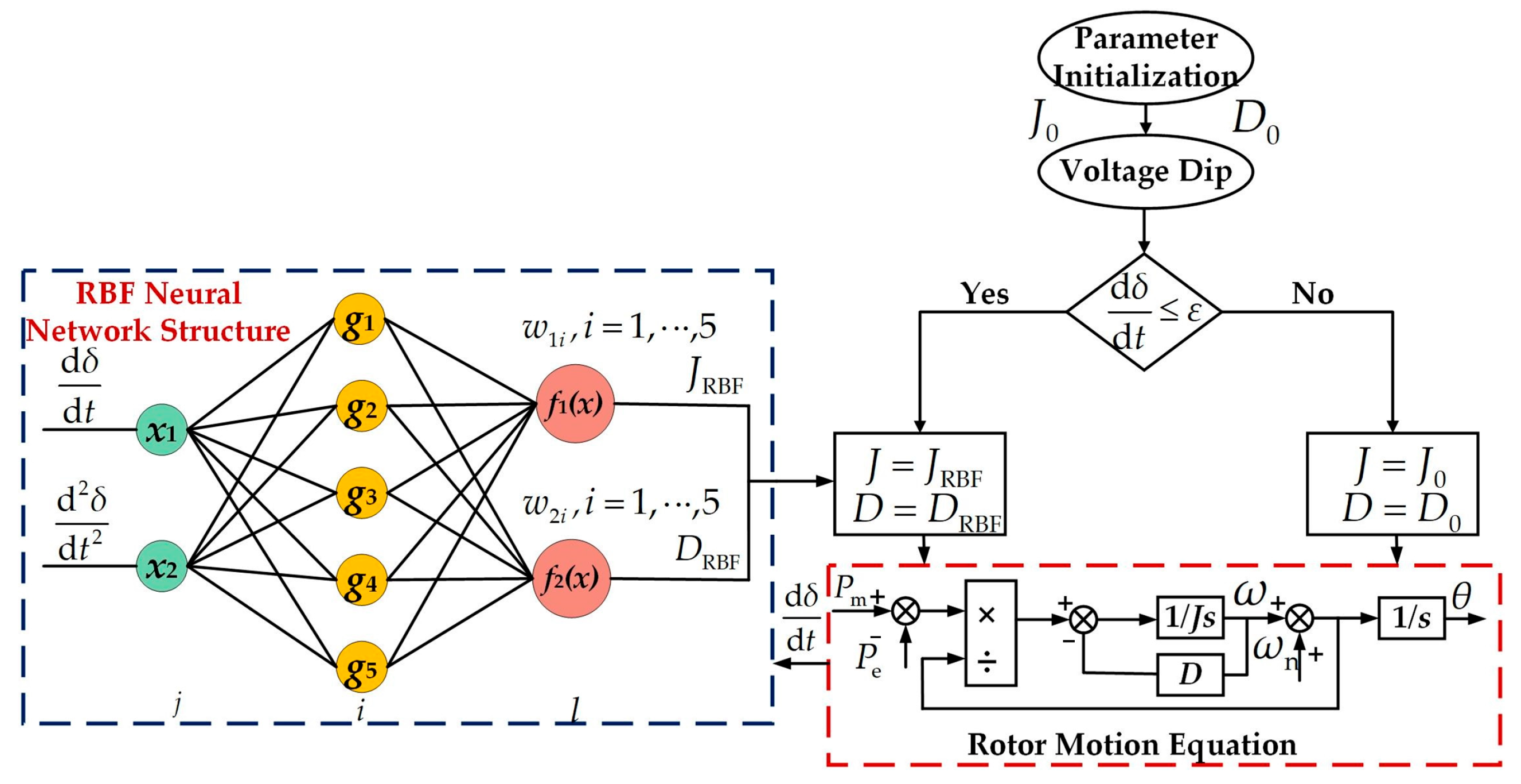
3.4. The Transient Power-Angle Control Strategy Based on RBF Neural Networks

The RBF neural network possesses strong adaptive capabilities, allowing it to adjust control parameters based on the real-time state of the system, making it especially suitable for addressing complex and nonlinear dynamic changes [31]. After a period of time following the fault occurrence, the system may enter a more stable transient process, where traditional control methods may no longer effectively adjust system parameters, or due to significant changes in the system’s state, the effectiveness of traditional control strategies gradually weakens. During the fault recovery process, due to the switching of control strategies and the introduction of virtual impedance, the attack angle will fluctuate. Therefore, based on the parameter characteristics of $J$ and $D$, the use of an RBF neural network can find the optimal adjustment strategy under changing system conditions, enhancing the dynamic stability of the system.

This paper adopts an RBF neural network with a 2-5-2 structure, where the input variables of the neural network are ${\displaystyle \frac{\mathrm{d}\mathsf{\delta }}{\mathrm{d}t}}$ and ${\displaystyle \frac{{\mathrm{d}}^2\mathsf{\delta }}{\mathrm{d}{t}^2}}$, represented by $x_1$ and $x_2$, respectively. The activation function of the hidden layer is a Gaussian function, and the output layer corresponds to the virtual inertia $J_{\mathrm{RBF}}$ and damping coefficient $D_{\mathrm{RBF}}$ of the VSG. The number of nodes in the input layer, hidden layer, and output layer are 2, 5, and 2, respectively. The dynamic adjustment of the VSG structure based on the RBF neural network is shown in Figure 8.

From Figure 8, it can be seen that the expression for the output of the input layer is:

$$O_j^{(1)}=x(j),j=1,2$$

(20)

where $O_j^{(1)}$ represents the output function of the input layer; $x(1)={\displaystyle \frac{\mathrm{d}\mathsf{\delta }}{\mathrm{d}t}}$, $x(2)={\displaystyle \frac{{\mathrm{d}}^2\mathsf{\delta }}{\mathrm{d}{t}^2}}$; and the superscript (1) denotes the input layer.

The input and output of the hidden layer are as follows:

$$N_i^{(2)}=x,x=\left[x(1),x(2)\right]$$

(21)

$$O_i^{(2)}(k)=g(N_i^{(2)}(k)),i=1,2,\cdots ,5$$

(22)

where $O_i^{(2)}(k)$ represents the output function of the hidden layer, $g(\cdot )$ is the Gaussian function, and the superscript (2) denotes the hidden layer.

$$g(x)=\exp (-{\displaystyle \frac{{‖x-c_i‖}^2}{2b_i^2}})$$

(23)

where $b_i={\left[b_1,b_2,\cdots ,b_5\right]}^{\mathrm{T}}$ represents the width vector of the Gaussian function, and $c_i=\left[c_{i1},c_{i2}\right]$ is the center vector of the $i$-th hidden layer.

The input to the output layer is:

$$N_i^{(3)}(k)={\displaystyle \sum _{i=1}^5{w}_{\mathit{li}}^{(3)}{O}_i^{(2)}(k)}$$

(24)

where $w_{\mathit{li}}^{(3)}$ represents the weight from the hidden layer to the output layer, and the superscript (3) denotes the output layer.

The output of the neural network’s output layer is:

$$J_{\mathrm{RBF}}=O_l^{(3)}(k)=f(N_l^{(3)}(k)),l=1$$

(25)

$$D_{\mathrm{RBF}}=O_l^{(3)}(k)=f(N_l^{(3)}(k)),l=2$$

(26)

where $O_l^{(3)}(k)$ represents the output function of the output layer.

The activation function of the output layer is:

$$f(\mathrm{x})={\displaystyle \frac{u_l{e}^x}{e^x+e^{-x}}},l=1,2$$

(27)

where $u_1$ represents the upper limit of the virtual inertia, and $u_2$ represents the upper limit of the damping coefficient.

The evaluation function of the neural network is:

$$E\left(k\right)={\displaystyle \frac{1}{2}}{[{\omega }_{\mathrm{n}}(k)-\omega (k)]}^2$$

(28)

This paper uses the gradient descent method to adjust the network weights. To improve the convergence speed, an inertia term is added to the equation, as follows:

$$\Delta w_{\mathit{li}}^{(3)}(k)=-\mathsf{\eta }{\displaystyle \frac{\mathsf{\partial }E(k)}{\mathsf{\partial }{w}_{\mathit{li}}^{(3)}}}+\alpha \Delta w_{\mathit{li}}^{(3)}(k-1)$$

(29)

$${\displaystyle \frac{\mathsf{\partial }E(k)}{\mathsf{\partial }{w}_{1i}^{(3)}}}={\displaystyle \frac{\mathsf{\partial }E(k)}{\mathsf{\partial }\omega (k)}}•{\displaystyle \frac{\mathsf{\partial }\omega (k)}{\mathsf{\partial }{J}_{\mathrm{RBF}}(k)}}•{\displaystyle \frac{\mathsf{\partial }{J}_{\mathrm{RBF}}(k)}{\mathsf{\partial }{N}_1^{(3)}(k)}}•{\displaystyle \frac{\mathsf{\partial }{N}_1^{(3)}(k)}{\mathsf{\partial }{w}_{1i}^{(3)}}}$$

(30)

$${\displaystyle \frac{\mathsf{\partial }E(k)}{\mathsf{\partial }{w}_{2i}^{(3)}}}={\displaystyle \frac{\mathsf{\partial }E(k)}{\mathsf{\partial }\omega (k)}}•{\displaystyle \frac{\mathsf{\partial }\omega (k)}{\mathsf{\partial }{D}_{\mathrm{RBF}}(k)}}•{\displaystyle \frac{\mathsf{\partial }{D}_{\mathrm{RBF}}(k)}{\mathsf{\partial }{N}_2^{(3)}(k)}}•{\displaystyle \frac{\mathsf{\partial }{N}_2^{(3)}(k)}{\mathsf{\partial }{w}_{2i}^{(3)}}}$$

(31)

where $\mathsf{\eta }$ represents the learning rate, and $\alpha$ represents the inertia coefficient.

Since $w(k)/J_{\mathrm{RBF}}(k)$ and $w(k)/D_{\mathrm{RBF}}(k)$ must be applied during the weight update process and their derivation is relatively complex, the perturbation method and the sign function method are used ${\displaystyle \frac{\mathsf{\partial }\omega (k)}{\mathsf{\partial }{J}_{\mathrm{RBF}}(k)}}$ and ${\displaystyle \frac{\mathsf{\partial }\omega (k)}{\mathsf{\partial }{D}_{\mathrm{RBF}}(k)}}$ can be expressed as follows:

$${\displaystyle \frac{\mathsf{\partial }\omega (k)}{\mathsf{\partial }{J}_{\mathrm{RBF}}(k)}}=\mathrm{sign}\left[{\displaystyle \frac{\omega (k)-\omega (k-1)}{J_{\mathrm{RBF}}(k)-J_{\mathrm{RBF}}(k-1)}}\right]$$

(32)

$${\displaystyle \frac{\mathsf{\partial }\omega (k)}{\mathsf{\partial }{D}_{\mathrm{RBF}}(k)}}=\mathrm{sign}\left[{\displaystyle \frac{\omega (k)-\omega (k-1)}{D_{\mathrm{RBF}}(k)-D_{\mathrm{RBF}}(k-1)}}\right]$$

(33)

In summary, the weight adjustment of the RBF neural network is as follows:

$$\begin{array}{l}\Delta w_{\mathit{li}}^{(3)}(k)=\mathsf{\eta }({\omega }_{\mathrm{n}}(k)-\omega (k))•\mathrm{sign}\left[{\displaystyle \frac{\omega (k)-\omega (k-1)}{J_{\mathrm{RBF}}(k)-J_{\mathrm{RBF}}(k-1)}}\right]•\\ f(N_l^{(3)}(k))•O_i^{(2)}(k)+\alpha \Delta w_{\mathit{li}}^{(3)}(k-1),i=1,\cdots ,5,l=1\end{array}$$

(34)

$$\begin{array}{l}\Delta w_{\mathit{li}}^{(3)}(k)=\mathsf{\eta }({\omega }_{\mathrm{n}}(k)-\omega (k))•\mathrm{sign}\left[{\displaystyle \frac{\omega (k)-\omega (k-1)}{D_{\mathrm{RBF}}(k)-D_{\mathrm{RBF}}(k-1)}}\right]•\\ f(N_l^{(3)}(k))•O_i^{(2)}(k)+\alpha \Delta w_{\mathit{li}}^{(3)}(k-1),i=1,\cdots ,5,l=2\end{array}$$

(35)

In summary, to avoid insufficient accuracy of the RBF neural network and oscillations caused by poor dynamic performance during the early stages of training, this paper adopts a switching mechanism based on the rate of change in the power angle. Specifically, when a voltage sag is detected, the rate of change in the power angle is compared with a threshold value $\mathsf{\epsilon }$. Once the system enters a stable or semi-stable state, it switches to the RBF neural network for adaptive adjustment. The threshold value, virtual inertia, and damping coefficient should be selected according to the specific conditions of the power grid [32,33,34]. In this paper, the values are chosen as $\mathsf{\epsilon }=1\times {10}^{-6}$, $J_{\max }=10J_0$, $D_{\max }=1.9D_0$ respectively. This approach not only maintains a fast response during the initial control phase but also improves the system’s stability and recovery performance in the later stages through adaptive adjustment by the neural network.

4. Simulation Analysis

4.1. Simulation System

To verify the superiority of the proposed RBF neural network-based dynamic control strategy, a system structure as shown in Figure 1 was established in MATLAB/Simulink R2023a. The simulation compares the proposed strategy with the traditional VSG fixed-parameter control strategy. Initially, the VSG operates in grid-connected mode under rated conditions. At 1.5 s, a fault is introduced, during which the voltage drops to 0.5 pu and 0.2 pu, respectively. At 3 s, the fault is cleared, and the total simulation time is 5 s. The simulation parameters are listed in

Table 2. Simulation parameters.

Symbols	Parameters	Value/Unit
$P_{\mathrm{m}}$	Rated active power	15/kW
$Q_{\mathrm{m}}$	Rated reactive power	0
$U_{\mathrm{g}}$	Grid voltage amplitude	311/V
$U_{\mathrm{dc}}$	DC-side voltage	1500/V
$I_{\lim }$	Current limit	1.5/pu
$L_{\mathrm{f}}$	Filter inductance	4/mH
$C_{\mathrm{f}}$	Filter capacitance	$10 \mathsf{\mu }\mathrm{F}$
${\omega }_{\mathrm{n}}$	Rated angular speed	314/rad/s
$J_0$	Rated virtual inertia	1 kg·m2
$D_0$	Rated dampingcoefficient	16/(N·m·s)/rad

.

Since the virtual impedance coefficient is related to the system recovery process and the transient current constraint determines the virtual impedance exponential coefficient, the relationship between the exponential coefficient and transient power-angle fluctuations as well as transient current surges is considered. Specifically, if the exponential coefficient is too large, the attenuation speed will be faster, leading to smaller transient power-angle fluctuations, but the resulting transient surge current will be larger. Conversely, if the exponential coefficient is too small, the transient surge current will be smaller, but the transient power-angle fluctuations will be larger, which is detrimental to system stability. Taking into account the surge current constraint of 1.5 pu and the characteristics of system parameters, the exponential coefficient is set to 5.

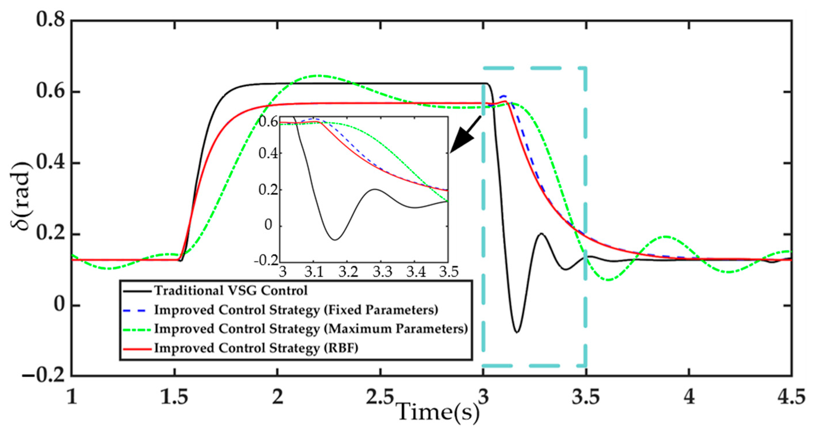
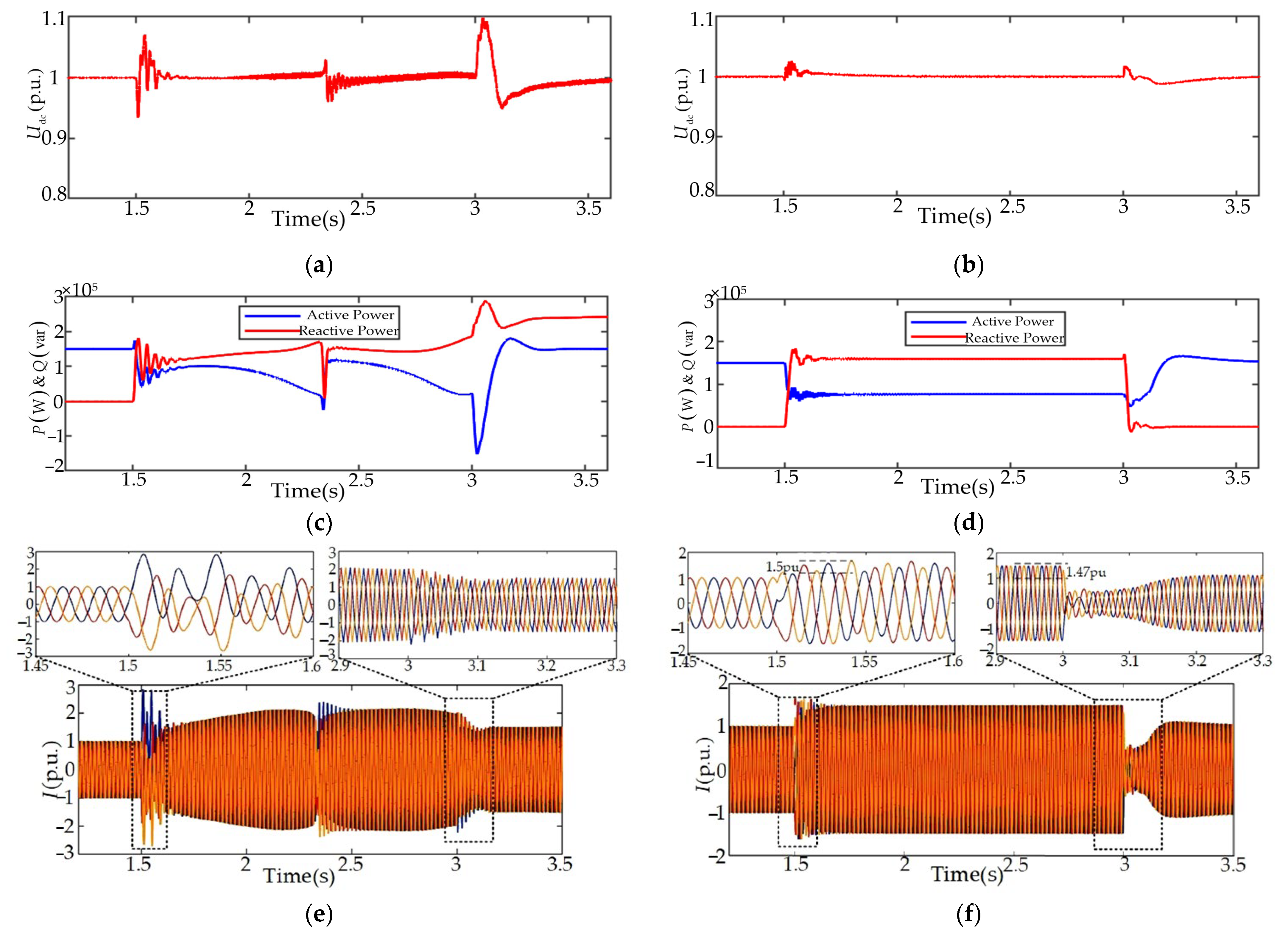
4.2. Validation of the Strategy Under Moderate Voltage Sag

First of all, when the grid voltage drops to 0.5 pu, the system’s transient responses under different control strategies are shown in Figure 9. By comparing Figure 9a,c with Figure 9b,d, it can be observed that after adopting the improved control strategy, the fluctuations in VSG output power and DC bus voltage are reduced, and the system’s power dynamic response is accelerated, demonstrating better transient. As shown in Figure 9f, the inverter output current during the fault and recovery phases is limited to 1.1 times the rated current, ensuring the safe operation of the VSG.

To verify the transient regulation characteristics of the proposed RBF neural network-based control strategy, a comparison was conducted among the traditional VSG control, fixed-parameter control, and the proposed control strategy, as shown in Figure 10. The incremental change in output power angle and the settling time are used as quantitative performance indicators for dynamic performance analysis. The analysis metrics for each algorithm are shown in

Table 3. Analysis indicators of different control strategies under moderate voltage sag.

Control Strategy	$\Delta \delta /\mathbf{rad}$	${\mathit{t}}_{\mathbf{s}}/\mathbf{s}$
Fixed Parameters	0.54	0.82
RBF	0.52	0.79

. The traditional VSG control exhibited significant transient power-angle overshoot and oscillations after fault clearance, with a maximum power-angle peak of approximately 0.62 rad, and a slow recovery speed. The improved fixed-parameter control strategy partially suppressed the overshoot and reduced the oscillation amplitude, with a maximum power-angle peak of approximately 0.54 rad, but its dynamic adjustment capability remained limited, and the recovery speed was still inadequate. In the case of improved maximum parameters, the overshoot during the fault period is relatively large, and the settling time is very long. Even after fault clearing, it is difficult to restore stability. In contrast, the RBF neural network-based adaptive control strategy significantly improved the transient power-angle characteristics through dynamic regulation, with a maximum power-angle peak of approximately 0.52 rad. It responded rapidly within 0.1 s after the fault occurrence, with the smoothest power-angle variation, and the system quickly returned to a stable state within approximately 0.79 s after the fault. This not only effectively suppressed the overshoot and oscillations after fault clearance but also accelerated the recovery speed of the power angle, thereby significantly enhancing the transient regulation performance of the system.

Under moderate voltage sag, the dynamic values of the neural network are shown in Figure 11. After the control strategy switches, the RBF neural network demonstrates rapid response characteristics. During the early stage of fault recovery, the increase in virtual inertia enhances the system’s disturbance rejection capability, while the dynamic adjustment of the damping coefficient further improves the system’s transient stability. In the mid-stage of fault recovery, the RBF neural network adaptively adjusts based on the system’s operating conditions, thereby accelerating the recovery process and effectively avoiding energy waste caused by overcompensation. Subsequently, the two parameters gradually return to appropriate values, enhancing the system’s transient regulation performance.

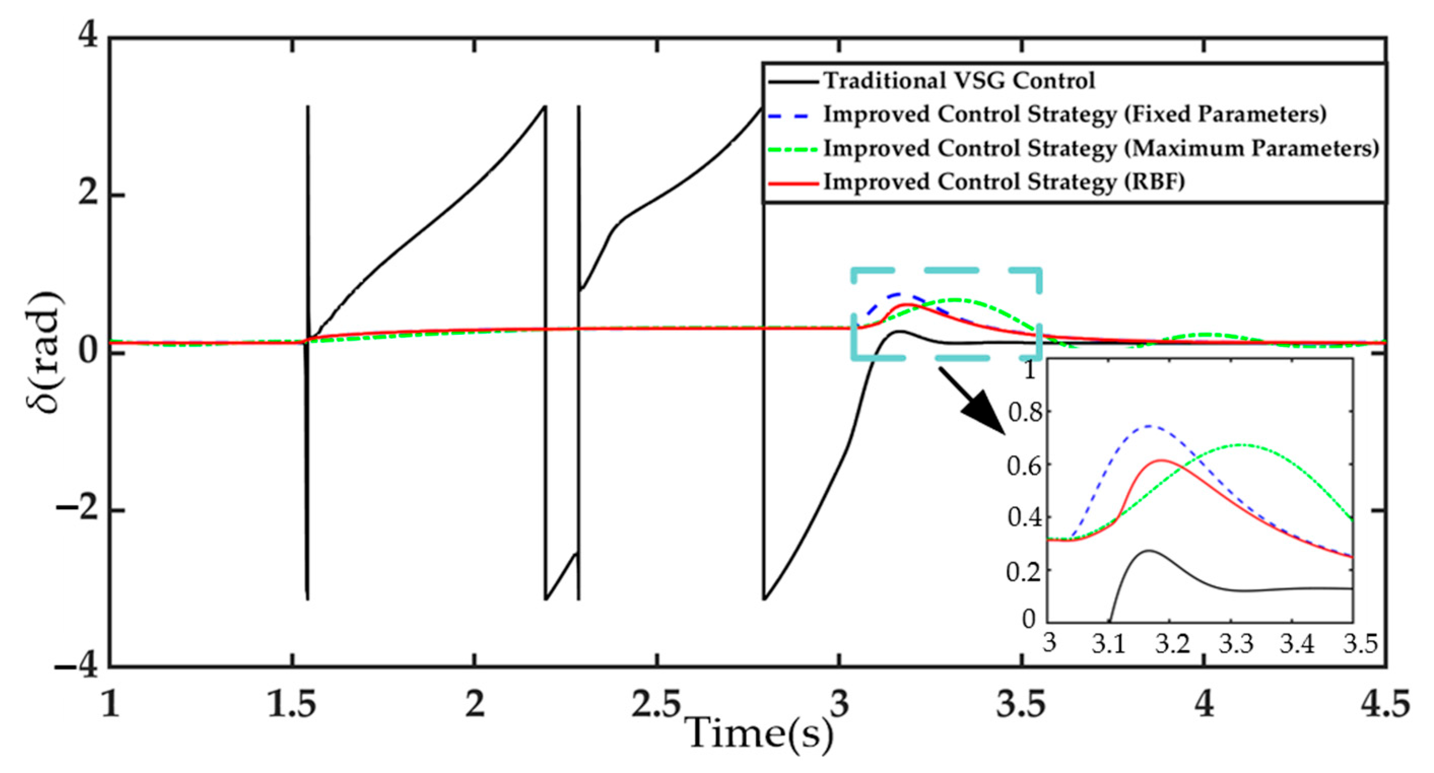
4.3. Validation of the Strategy Under Severe Voltage Sag

When the grid voltage drops to 0.2 pu, the transient responses of the system under different control strategies are shown in Figure 12. From the comparison of Figure 12a,c and Figure 12b,d, it can be concluded that the system becomes unstable under the traditional VSG control strategy. However, with the improved control strategy, the fluctuations in power and bus voltage are significantly reduced, and active and reactive power are actively adjusted during the fault period. According to Figure 12f, the inverter output current is strictly limited to within 1.5 times the rated current throughout the entire fault duration, effectively ensuring the safe operation of the VSG.

Figure 13 shows the transient power-angle characteristics under severe voltage sag for the traditional VSG control, fixed-parameter control, and the proposed control strategy. After the fault occurs, the power-angle peak of the traditional VSG control reaches approximately 3.4 rad, with large oscillation amplitudes and prolonged oscillation duration, indicating significant instability. The evaluation metrics under severe voltage sag conditions are shown in

Table 4. Analysis indicators of different control strategies under severe voltage sag.

Control Strategy	$\Delta \delta /\mathbf{rad}$	${\mathit{t}}_{\mathbf{s}}/\mathbf{s}$
Fixed Parameters	0.43	0.61
RBF	0.26	0.61

. The improved fixed-parameter control strategy effectively enhances system stability, but during the fault recovery period, the power-angle peak reaches approximately 0.78 rad, offering limited performance improvement. In the case of improved maximum parameters, the recovery speed of the angle of attack is slow, and it cannot return to its initial value within a short period of time. In contrast, the RBF-based improved control strategy not only ensures system stability but also reduces the power-angle peak to approximately 0.61 rad, while the recovery time remains 0.61 s.

The dynamic values of the neural network under severe voltage sag are shown in Figure 14. Considering the learning characteristics of the neural network, which need to adapt to the dynamic changes in system states, the virtual inertia $J$ exhibits slight oscillations after switching control strategies. However, due to its rapid learning capability, it significantly improves the system’s dynamic response during fault recovery, providing superior transient performance and adaptive capability for complex and dynamic power grids.

5. Conclusions

To improve the transient stability of VSGs under symmetrical grid faults, this paper establishes a GFM photovoltaic system. A LVRT control strategy based on RBF neural networks combined with dynamic virtual impedance is proposed to address inverter overcurrent issues and transient power-angle recovery characteristics during voltage sags. This contributes to both the economic and environmental goals of increasing renewable energy capacity while maintaining grid security and reliability. The following conclusions are drawn through simulations:

(1)

In the early stages of fault recovery, larger virtual inertia and damping coefficients effectively suppress transient power-angle overshoot. In the mid-recovery period, smaller virtual inertia and damping coefficients improve the power-angle recovery speed.

(2)

Virtual impedance helps to suppress transient current surges. Dynamic virtual impedance, which takes into account the voltage sag severity and inverter overcurrent capacity, not only mitigates transient current but also enhances system stability.

(3)

The RBF neural network, with its rapid learning capability and adaptive adjustment features, significantly improves transient power-angle recovery characteristics and enhances the system’s transient control performance. Future work will focus on optimizing the RBF neural network-based control strategy to enhance the robustness and recovery speed of the photovoltaic system under asymmetrical fault conditions.

References

1. Zhuo, Z.; Zhang, N.; Xie, X.; Li, H.; Kang, C. Key technologies and developing challenges of power system with high proportion of renewable energy. Autom. Electr. Power Syst. 2021, 45, 171–191. (In Chinese) [Google Scholar]
2. Yuan, H.; Song, X.; Sun, F.; Xin, X.; Huang, L.; Guan, Z. Analysis of LVRT control strategy-oriented DFIG instability mechanism in weak grid. Electr. Power Autom. Equip. 2020, 40, 50–56. (In Chinese) [Google Scholar]
3. Pan, H.C.X.; Huang, H.; Sun, X.; He, D.; Yong, C. Equivalent modeling of LVRT and current limiting links for distributed photovoltaic and wind turbine generators. Electr. Power Autom. Equip. 2022, 42, 3–10. (In Chinese) [Google Scholar]
4. Li, H.; Li, S.; Tang, M.; Su, Q. Control strategy of renewable energy inverter considering voltage sag degree under asymmetric faults. Power Syst. Prot. Control. 2023, 51, 21–32. (In Chinese) [Google Scholar]
5. Wang, S.; Liu, F.; Zhuang, Y.; Liu, Q.; Huang, Y.; Zha, X. Active-power-command-sharing low-voltage ride-through control strategy for two-stage PV grid-connected system. Electr. Power Autom. Equip. 2023, 43, 99–105. (In Chinese) [Google Scholar]
6. Zhang, Z.; Zhang, L.; Wang, B.; Zhou, H. Research on LVRT control strategy for two-stage three-phase grid-connected inverter. Power Electron. 2017, 51, 73–75. (In Chinese) [Google Scholar]
7. Naik, K.R.; Rajpathak, B.; Mitra, A.; Kolhe, M.L. Adaptive energy management strategy for sustainable voltage control of PV-hydro-battery integrated DC microgrid. J. Clean. Prod. 2021, 315, 128102, ISSN 0959-6526. [Google Scholar] [CrossRef]
8. Naik, K.R.; Rajpathak, B.; Mitra, A.; Kolhe, M.L. Assessment of energy management technique for achieving the sustainable voltage level during grid outage of hydro generator interfaced DC Micro-Grid. Sustain. Energy Technol. Assess. 2021, 46, 101231, ISSN 2213-1388. [Google Scholar] [CrossRef]
9. Sebaa, K.; Zhou, Y.; Li, Y.; Gelen, A.; Nouri, H. Low-frequency Oscillation Damping Control for Large-scale Power System with Simplified Virtual Synchronous Machine. J. Mod. Power Syst. Clean. Energy 2021, 9, 1424–1435. [Google Scholar] [CrossRef]
10. D’Arco, S.; Suul, J.A.; Fosso, O.B. Control system tuning and stability analysis of Virtual Synchronous Machines. In Proceedings of the IEEE Energy Conversion Congress and Exposition, Denver, CO, USA, 15–19 September 2013; pp. 2664–2671. [Google Scholar]
11. Zhang, K.; Wang, G.; GENG, X.; Jia, Z.; Li, X.; Shen, Y. Distributed cooperative control strategy for grid connected power in ADN with high proportion of PVESS units. J. Electr. Power Sci. Technol. 2022, 37, 147–155. (In Chinese) [Google Scholar]
12. Chen, T.; Chen, L.; Zheng, T.; Mei, S. LVRT control method of virtual synchronous generator based on mode smooth switching. Power Syst. Technol. 2016, 40, 2134–2140. (In Chinese) [Google Scholar]
13. Chen, L.; Zhang, X.; Dang, X.; Li, J.; Feng, T. Low-voltage ride-through control of photovoltaic virtual synchronous generator using new model prediction. J. Power Supply 2024, 22, 163–172. (In Chinese) [Google Scholar]
14. Wang, P.; Wang, P.; Li, K.; Wang, W.; Xu, D. Dynamic current-limiting control strategy of grid-forming inverter under grid faults. High. Volt. Eng. 2022, 48, 3829–3837. (In Chinese) [Google Scholar]
15. Wong, Y.C.C.; Lim, C.S.; Cruden, A.; Rotaru, M.D.; Ray, P.K. A Consensus-Based Adaptive Virtual Output Impedance Control Scheme for Reactive Power Sharing in Radial Microgrids. IEEE Trans. Ind. Appl. 2021, 57, 784–794. [Google Scholar] [CrossRef]
16. Paquette, A.D.; Divan, D.M. Virtual Impedance Current Limiting for Inverters in Microgrids with Synchronous Generators. IEEE Trans. Ind. Appl. 2015, 51, 1630–1638. [Google Scholar] [CrossRef]
17. Jia, K.; Liu, Y.; Bi, T.; Zhang, Y. Asymmetric fault ride-through control of grid-connected renewable energy sources based on adaptive virtual impedance. Proc. CSEE 2024, 44, 1–11. (In Chinese) [Google Scholar]
18. Li, Q.; Ge, P.; Xiao, F.; Lan, Z.; Ge, Q. Study on fault ride-through method of VSG based on power angle and current flexible regulation. Proc. CSEE 2020, 40, 2071–2080. (In Chinese) [Google Scholar]
19. Li, J.; Wen, B.; Wang, H. Adaptive Virtual Inertia Control Strategy of VSG for Micro-Grid Based on Improved Bang-Bang Control Strategy. IEEE Access 2019, 7, 39509–39514. [Google Scholar] [CrossRef]
20. Yang, H.; Jia, Q.; Xiang, L.; Yan, G.; Zhang, S.; Li, X. Virtual inertia control strategies for double-stage photovoltaic power generation. Autom. Electr. Power Syst. 2019, 43, 87–94. (In Chinese) [Google Scholar]
21. Li, X.; Jia, Q.; Xiang, L.; Tian, B. Two-stage photovoltaic generation actively participating in grid frequency regulation. Power Syst. Prot. Control. 2019, 47, 100–110. (In Chinese) [Google Scholar]
22. Yin, G.; Dong; Dai, Y.; Wang, H.; Wang, S. Adaptive control strategy of VSG parameters in photovoltaic Microgrids. Power Syst. Technol. 2020, 44, 192–199. (In Chinese) [Google Scholar]
23. Yao, F.; Zhao, J.; Li, X.; Mao, L.; Qu, K. RBF Neural Network Based Virtual Synchronous Generator Control with Improved Frequency Stability. IEEE Trans. Ind. Inform. 2021, 17, 4014–4024. [Google Scholar] [CrossRef]
24. Li, X.; Wang, L.; Yan, N.; Ma, R. Cooperative Dispatch of Distributed Energy Storage in Distribution Network with PV Generation Systems. IEEE Trans. Appl. Supercond. 2021, 31, 8. [Google Scholar] [CrossRef]
25. Sher, H.A.; Murtaza, A.F.; Noman, A.; Addoweesh, K.E.; Al-Haddad, K.; Chiaberge, M. A New Sensorless Hybrid MPPT Algorithm Based on Fractional Short-Circuit Current Measurement and P&O MPPT. IEEE Trans. Sustain. Energy 2015, 6, 1426–1434. [Google Scholar]
26. Mo, O.; D’Arco, S.; Suul, J.A. Evaluation of Virtual Synchronous Machines with Dynamic or Quasi-Stationary Machine Models. IEEE Trans. Ind. Electron. 2017, 64, 5952–5962. [Google Scholar] [CrossRef]
27. Tang, Y.; Tian, Z.; Zha, X.; Li, X.; Huang, M.; Sun, J. An Improved Equal Area Criterion for Transient Stability Analysis of Converter-Based Microgrid Considering Nonlinear Damping Effect. IEEE Trans. Power Electron. 2022, 37, 11272–11284. [Google Scholar] [CrossRef]
28. Ma, J.; Ding, X.; Lin, X.; Huang, T.; Wang, Z. Three-phase short circuit current calculation considering converter transient regulation for doubly-fed wind-power generator. Electr. Power Autom. Equip. 2016, 36, 129–136. (In Chinese) [Google Scholar]
29. GB/T 19964-2024; Technical requirements for connecting photovoltaic power station to power system. State Administration for Market Regulation: Beijing, China, 2024.
30. Gan, M.; Chen, X.-X.; Ding, F.; Chen, G.-Y.; Chen, C.L.P. Adaptive RBF-AR Models Based on Multi-Innovation Least Squares Method. IEEE Signal Process. Lett. 2019, 26, 1182–1186. [Google Scholar] [CrossRef]
31. Wang, Y.; Yang, L.; Yu, Y.; MA, B. Coordination and optimization strategy of virtual inertia and damping coefficient of a virtual synchronous generator. Power Syst. Prot. Control. 2022, 50, 88–98. (In Chinese) [Google Scholar]
32. Xing, D.; Tian, M. Relationship between frequency characteristics of virtual synchronous generator and parameters of energy storage equipment. Power Syst. Technol. 2021, 45, 3582–3590. (In Chinese) [Google Scholar]
33. Lu, S.; Zhu, Y.; Chen, T.; Wang, T.; Wang, N. Adaptive control strategy of damping inertia based on improved particle swarm optimization algorithm. Proc. CSU-EPSA 2024, 36, 68–75. (In Chinese) [Google Scholar]
34. Huang, X.; Liang, Q.; Chen, X.; Li, W.; Teng, J. Fuzzy adaptive control strategy for interface converter parameter based on VSG. J. Guangxi Univ. (Nat. Sci. Ed.) 2024, 49, 360–373. (In Chinese) [Google Scholar]
Figure 1. Topology of the main circuit and control system of the GFM photovoltaic system.
Electronics 14 00785 g001
Figure 2. The photovoltaic energy storage control strategy.
Electronics 14 00785 g002
Figure 3. VSG power-angle characteristics for different fault severities.
Electronics 14 00785 g003
Figure 4. VSG power-angle characteristics for different active power command values: (a) rated active power value; (b) increase in active power command value.
Electronics 14 00785 g004
Figure 5. VSG power loop control block diagram; (a) Active power–frequency control loop; (b) Reactive power–voltage control loop.
Electronics 14 00785 g005
Figure 6. VSG phase plane diagram under different control parameters: (a) different active power command values; (b) different virtual inertia values; (c) different damping coefficients.
Electronics 14 00785 g006
Figure 7. Dynamic virtual impedance adjustment diagram.
Electronics 14 00785 g007
Figure 8. Dynamic adjustment and optimization structure of VSG parameters.
Electronics 14 00785 g008
Figure 9. Transient response of VSG and improved control strategies under moderate voltage sag level: (a) DC bus voltage under the VSG control strategy; (b) DC bus voltage under the improved control strategy; (c) output power under the VSG control strategy; (d) output power under the improved control strategy; (e) output current under the VSG control strategy; (f) output current under the improved control strategy.
Electronics 14 00785 g009
Figure 10. Transient power-angle characteristics under moderate voltage sag.
Electronics 14 00785 g010
Figure 11. Dynamic values of J RBF and D RBF under moderate voltage sag: (a) values of virtual inertia J RBF ; (b) values of the damping coefficient D RBF .
Electronics 14 00785 g011
Figure 12. Transient response of VSG and improved control strategies under severe voltage sag level: (a) DC bus voltage under the VSG control strategy; (b) DC bus voltage under the improved control strategy; (c) output power under the VSG control strategy; (d) output power under the improved control strategy; (e) output current under the VSG control strategy; (f) output current under the improved control strategy.
Electronics 14 00785 g012
Figure 13. Transient power-angle characteristics under severe voltage sag.
Electronics 14 00785 g013
Figure 14. Dynamic values of J RBF and D RBF under severe voltage sag: (a) values of virtual inertia J RBF ; (b) values of the damping coefficient D RBF .
Electronics 14 00785 g014