Fast Multi-View Subspace Clustering Based on Flexible Anchor Fusion

Abstract

Multi-view subspace clustering enhances clustering performance by optimizing and integrating structural information from multiple views. Recently, anchor-based methods have made notable progress in large-scale clustering scenarios by leveraging anchor points to capture data distribution across different views. Although these methods improve efficiency, a common limitation is that they typically select an equal number of anchor points from each view. Additionally, during the graph fusion stage, most existing frameworks use simple linear weighting to construct the final consensus graph, overlooking the inherent structural relationships between the data. To address these issues, we propose a novel and flexible anchor graph fusion framework which selects an appropriate number of anchor points for each view based on its data space, creating suitable anchor graphs. In the graph fusion stage, we introduce a regularization term which adaptively and flexibly combines anchor graphs of varying sizes. Moreover, our approach incorporates both global and local information between views, enabling a more accurate capture of the cluster structure within the data. Furthermore, our method operates with linear time complexity, making it well suited for large-scale datasets. Extensive experiments on multiple datasets demonstrate the superior performance of our proposed algorithm.

1. Introduction

With the rapid advancement of information technology, diverse, high-dimensional data from multiple sources are increasingly being generated in real-world scenarios [1,2]. Such data are often referred to as multi-view data, as they are collected from different perspectives or modalities, including various sensors, feature descriptors, or languages [3,4,5,6,7]. For example, an image can be described by different features like local binary patterns (LBPs), histograms of oriented gradients (HOGs), and Gabor descriptors [3], while a news article might be available in different languages like Chinese, English, and Spanish [8]. Similarly, a video clip can be broken down into visual frames, audio tracks, and textual descriptions, each collected from distinct sources [9,10]. The challenge of effectively leveraging the complementary information contained in these multiple views has driven the development of numerous multi-view clustering (MVC) approaches. Among them, subspace-based clustering techniques have gained significant interest due to their ability to efficiently reveal hidden data structures and uncover the intrinsic relationships among data pairs. Multi-view subspace clustering (MVSC), as a well-known unsupervised approach, has demonstrated great effectiveness in data mining and knowledge discovery, providing robust clustering results by integrating diverse and complementary information from multiple views [11,12,13,14].

Various MVSC methods often adopt the following framework: (1) in each view, learning a low-dimensional representation matrix or similarity matrix through subspace learning; (2) integrating and fusing all view-specific subspace representations to find a shared subspace which reflects the intrinsic structure of the data; and (3) using spectral clustering to derive the final clustering results. For example, Lan et al. [15] addressed feature degeneration by jointly learning consensus and view-specific subspaces, and Ma et al. [16] enhanced clustering quality through automatic neighbor discovery and an improved similarity matrix without hyperparameters.

Despite the improvements in MVSC methods above, these algorithms often suffer from high complexity, requiring significant computational and spatial resources [17]. This high complexity arises from two key steps. (1) In the single-view subspace construction and optimization phase, the learned low-dimensional representation matrix in each view is typically obtained using a self-representation strategy, leading to quadratic space complexity and cubic time complexity with respect to the number of samples. (2) In the fusion and clustering phase, after obtaining the fused subspace representation matrix, the clustering phase involves spectral clustering, which requires singular value decomposition (SVD) and takes a time complexity of $O\left(n^3\right)$. For example, Maria et al. [18] proposed a multi-view subspace clustering method which learns joint subspace representation by constructing a shared association matrix. It combines a low rank constraint and sparse constraint to improve the clustering accuracy. Lu et al. [19] proposed a unified subspace clustering method by introducing block diagonal matrix regularization, directly pursuing the block’s diagonal structure to obtain clustering results. Although these methods have achieved good clustering effects, their time complexity of $O\left(n^2\right)$ or $O\left(n^3\right)$ hinders the application to large-scale scenarios.

In recent years, anchor graph algorithms have been proposed to accelerate multi-view subspace clustering, aiming to reduce complexity and extend its applicability to large-scale clustering tasks [20,21,22]. Typically, anchors are chosen or sampled independently in each view, using methods such as k-means clustering, random sampling, or DPP sampling. By independently sampling the anchor points for each view, the global matrix of $d\times n$ can be transformed into the anchor points matrix of $d\times m$, where m represents the amount of selected anchor points and $m<<n$. After the single-view subspace construction phase, a weighted linear combination of the anchor graphs or similarity matrices from each view is typically formed to obtain a fused graph. Due to their efficiency, many MVSC methods based on anchor point strategies have been proposed. For example, Wang et al. [23] integrated anchor selection and graph construction to enhance efficiency and clustering quality. Zhou et al. [1] effectively extracted representative anchor points by combining the eigenvalues of each sample, which helps avoid instability in methods like k-means clustering, and then the clustering results can be obtained directly based on the connectivity of the fused graph, eliminating the instability of clustering results. Moreover, the time complexity and space complexity can be regarded as $O\left(n\right)$, which is suitable for large-scale clustering tasks.

However, anchor-based multi-view subspace clustering methods can still be further improved. First, many methods separate the anchor graph construction and graph fusion processes into two independent steps, which may result in the loss of consensus information during the final clustering, thereby reducing clustering performance. Secondly, many anchor-based methods focus on capturing the global structure of the data, specifically the relationships between the samples and all anchors. This often leads to a dense correspondence matrix. However, neglecting local structure information may result in the loss of complementary data between samples in the final fused consensus graph. Thirdly, current anchor-based methods require selection of the same number of anchors for each view, which is unrealistic due to the differing data distributions and representations across views. This discrepancy makes it challenging to determine an equal number of anchors which effectively represent the underlying data structure in all views. Furthermore, traditional weighted linear combination methods face difficulties in fusing anchor graphs of varying sizes. These limitations undermine the effectiveness and applicability of anchor point mechanisms in large-scale multi-view subspace clustering tasks.

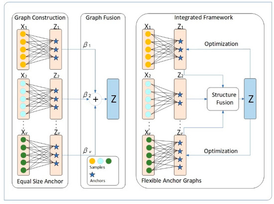
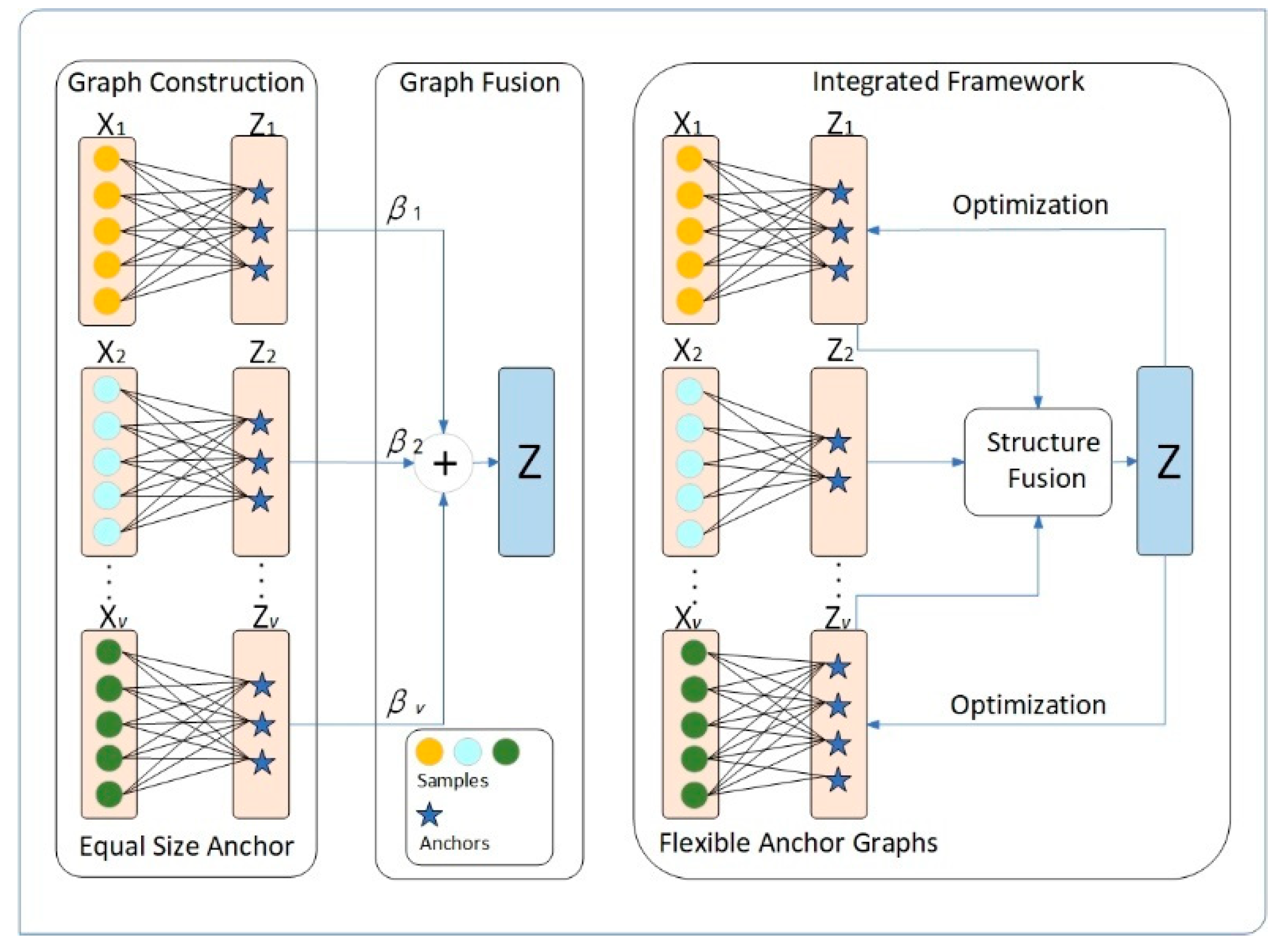
To enhance the effectiveness and flexibility of anchor-based MVSC methods, we propose a novel framework in Figure 1 called FMVSC, based on the flexible fusion of anchor graphs. Specifically, to address the issues mentioned above, we first integrate construction and optimization of the anchor matrix and anchor graph into a unified framework, which is iteratively updated based on the consensus and complementary information. This approach allows the components to better align with the underlying data space. Additionally, we not only focus on capturing the global structure of the data but also explore the local structure. Integrating both the global and local structures helps enhance the final clustering performance. More importantly, unlike traditional anchor-based methods, which rely on an equal number of anchors and a simple linear combination, we carefully examine existing anchor-based frameworks and introduce structure regularization for anchor graph fusion, developing a new structural alignment framework. From the perspective of anchor point constraints, traditional frameworks only select an equal number of anchors for each view, whereas our framework can learn anchor graphs which align with the data space of individual views, integrating consensus and complementary information between individual views. From the perspective of fusion strategies, simple linear combination strategies can only fuse anchor graphs of the same size, whereas our framework more flexibly fuses anchor graphs of different sizes, aggregating more comprehensive information.

Figure 1. (left) Existing anchor graph fusion strategy with equally sized anchors. (right) Our proposed FMVSC framework.

In addition, the time and space complexity of this method is linear, making it well suited for large-scale data applications. Comprehensive experiments on multiple benchmark datasets demonstrate that FMVSC outperforms current state-of-the-art methods in terms of both clustering performance and computational efficiency.

Overall, the primary contributions of this paper can be summarized in three key points:

(1)

Unlike existing frameworks, our proposed framework can automatically learn and update anchor points. We integrate the construction and optimization of the anchor matrix and anchor graph into a unified framework. By iteratively updating these components using consensus and complementary information, they can more accurately capture the underlying data structure.

(2)

We focus not only on capturing the global structure of the data but also exploring its local structure. Integrating both global and local structures helps to enhance the final clustering performance. Based on the global and local structures, we propose an alternative optimization method with linear complexity relative to the number of examples, and the experimental results demonstrate the effectiveness and efficiency of FMVSC.

(3)

Instead of using the same number of anchors, we believe that each view has its own unique underlying data space, and the number of anchors should be selected to match the characteristics of each view. Therefore, we propose a new framework which can learn anchor graphs that align with the data space of individual views and fuse anchor graphs of different sizes.

The remainder of this paper is organized as follows. Section 2 reviews the related work on multi-view subspace clustering and presents our proposed framework. Section 3 introduces the iterative optimization algorithm and discusses the time and space complexity, as well as the convergence issues of FMVSC. Section 4 presents the experimental results on benchmark datasets, comparing FMVSC with eight state-of-the-art multi-view clustering methods. Section 5 concludes the paper.

2. Related Work and Proposed Approach

2.1. Single-View Subspace Clustering

Subspace clustering assumes that high-dimensional data are distributed across several low-dimensional subspaces, with each class corresponding to a different subspace. Each data point can be represented by a linear combination of other points within the same subspace. For high-dimensional data, subspace clustering is an important unsupervised learning method. Based on the self-expression property of subspace clustering, many algorithms have been proposed to explore the underlying relationships among high-dimensional data. For example, in low-rank representation (LRR) [24], data recovery is achieved through low-rank representation. Sparse subspace clustering (SSC) [25] leverages the idea that sparse representation in high-dimensional subspaces better aligns with the structural model of the actual subspace. In a recent work, Nie et al. [26] improved subspace clustering by initializing the dictionary with partial samples, avoiding trivial solutions. The framework employs a bipartite graph to utilize the duality between samples and features, capturing subspace structures more effectively. Moreover, Nie introduced rank constraints and spare constraints to the framework, making it more effective and robust. The common single-view subspace clustering equation is shown in Equation (1) [27]:

$$\underset{Z}{\mathit{min}}\Vert X-XZ{\Vert }_F^2+\alpha \Vert Z{\Vert }_F^2$$

(1)

$$s.t. Z\ge 0, Z\mathbf{1}=1$$

where $Z\in R^{n\times n}$ denotes the nonnegative coefficient matrix. The second term is a regularization term, aiming to prevent trivial solutions.

2.2. Multi-View Subspace Clustering

Multi-view subspace clustering is the extension of single-view subspace clustering, which mainly improves the clustering accuracy by fully exploring the complementary and consensus information between views. Specifically, the MVSC approach typically adopts the following framework: Learn the low-dimensional representation matrix for each view, then learn a fused embedding matrix with consensus across all views. Finally, apply spectral clustering to obtain the final clustering result.

The common MVSC equation is shown in Equation (2) [28]:

$$\underset{Z_p}{\mathit{min}}{\displaystyle \sum }_{p=1}^v\Vert X_p-X_p{Z}_p{\Vert }_F^2+\lambda f\left(C,Z_p\right)$$

(2)

$$s.t. Z_p\ge 0, {Z_p}^T\mathbf{1}=1$$

where $f\left(·\right)$ represents the regularization function, $Z_p\in R^{n\times n}$ denotes the nonnegative self-representation matrix of each view, and $C$ represents the spectral embedding matrix of all views.

In some recent studies, efforts have been made to enhance the precision of subspace clustering. For example, Shi et al. [29] enhanced latent multi-view subspace clustering by constructing an augmented data matrix with block-diagonal and non-diagonal entries, capturing complementary and consistent information. Chen et al. [13] proposed a multimodal subspace clustering algorithm based on spatiotemporal attention to improve clustering performance by applying cross-modal learning and attention mechanisms. But these methods usually have high time complexity, which limits the application of MVSC methods on large-scale datasets.

2.3. Anchor-Based Multi-View Subspace Clustering

Recently, in order to alleviate the high time complexity of traditional MVSC methods and make better use of the potential information between views, many scholars have begun to conduct multi-view subspace clustering research based on anchor points. For instance, Kang et al. [21] first applied the anchor point strategy to large-scale subspace clustering, which achieves linear time complexity for large datasets and is also suitable for single-view scenarios. Zhao et al. [30] combined bipartite graphs, rank constraints, and the anchor point strategy to propose a scalable structured graph learning framework, while also systematically addressing the out-of-sample problem for the first time. Li et al. [31] proposed a parameter-free multi-view subspace clustering framework based on bipartite graphs and anchor graphs. It obtains a fused graph through self-supervised weighting, and due to the applied connectivity constraints, the clustering results can be directly obtained without postprocessing. Yang et al. [32] combined the anchor point strategy and spectral embedding decomposition to propose a robust and efficient framework. It improves clustering performance by constructing an anchor graph, which approximates the sample graph, and then decomposing the anchor graph. Lao et al. [33] generated diversified anchor point sets for each view and learns a bipartite graph for each view based on them. These bipartite graphs are then learned and segmented, ultimately producing a unified bipartite graph for clustering. This method also has linear time complexity.

Although the mentioned MVSC methods have achieved reasonable results, they all use an equal number of anchor points for graph construction in each view, which is reasonable, as each view has its own unique data space.

2.4. Spectral Clustering

Spectral clustering (SC) is widely used in the field of unsupervised learning [25]. Traditional spectral clustering methods are relatively simple and can easily obtain clustering results by performing k-means clustering on the low-dimensional embedding matrix of the data matrix. For a similarity graph $S\in R^{n\times n}$, the traditional SC equation can be represented as shown in Equation (3) [34]:

$$\underset{F^{T}F=I}{\mathit{max}}Tr\left(FS{F}^T\right)$$

(3)

where $F\in R^{k\times n}$ represents the low-dimensional spectral embedding matrix.

2.5. Proposed Approach

As mentioned above, most of the anchor-based multi-view clustering methods use k means clustering or random sampling to select the same number of anchor points in all views, carry out anchor graph learning, and finally obtain the consistent indicator matrix for clustering through simple weighted linear combination. Therefore, there is an underlying assumption in all these methods that an equal number of anchors can represent the latent data structure of each view in multi-view data. This is obviously irrational, as multi-view data are distributed and represented differently in each view, making it difficult to determine an equal number of anchor points to represent the latent data structure for all views. Moreover, facing the unique anchor graph built for each view, the traditional weighted linear combination method cannot fuse multiple anchor graphs of different sizes.

To solve these problems, we introduce a structural regularization term for fusing anchor graphs of different sizes in this paper. First of all, when reviewing Equation (3) in spectral clustering, we can notice that Equation (3) is equivalent to Equation (4) below:

$$\underset{F^{T}F=I}{\mathit{min}}\Vert S-F^{T}F{\Vert }_F^2$$

(4)

In Equation (5), we provide the related proof:

$$Equation \left(4\right)=\underset{F}{\mathit{min}}Tr\left(S{S}^T-2FS{F}^T+F^{T}FF{F}^T\right)=\underset{F}{\mathit{max}}Tr\left(FS{F}^T\right)=Equation \left(3\right)$$

(5)

Assume that all views share the same underlying clustering structure, which means all views share a uniform $F$, even if they do not have the same anchor graph size. Noting that $S$ in Equation (4) can be represented by $Z^{T}Z$ [21], in multi-view clustering methods, Equation (4) can be transformed into Equation (6):

$$min{\displaystyle \sum }_{p=1}^v\Vert {Z_p}^T{Z}_p-F^{T}F{\Vert }_F^2$$

(6)

In addition, in order to reduce the quadratic programming problems and high time complexity which may occur in the future, and to construct $Z_p$ such that it is more suitable for each data space, we introduce a rotation matrix $R_p\in R^{k\times l_p}$ satisfying ${R_p}^T{R}_p=I_{l_p}$. Then, Equation (6) can be rewritten as Equation (7) such that it is equivalent to Equation (7):

$$\begin{gathered} min{\displaystyle \sum }_{p=1}^v\Vert {Z_p}^T{R_p}^T{R}_p{Z}_p-F^{T}F{\Vert }_F^2 \\ s.t. Z_p\ge 0, {Z_p}^{T}1=1, {R_p}^T{R}_p=I_{l_p}, F{F}^T=I_k \end{gathered}$$

(7)

In order to further simplify the subsequent iterative update process and reduce the time complexity, we replace Equation (7) with Equation (8):

$$\begin{gathered} min{\displaystyle \sum }_{p=1}^v\Vert R_p{Z}_p-F{\Vert }_F^2 \\ s.t. Z_p\ge 0, {Z_p}^{T}1=1, {R_p}^T{R}_p=I_{l_p}, F{F}^T=I_k \end{gathered}$$

(8)

Let $C=R_p{Z}_p-F$. Then, we have proof in Equation (9) to make sure that the minimum value of Equation (7) can be obtained approximately by minimizing Equation (8), and $\Vert F{\Vert }_F=k^{{\displaystyle \raisebox{1ex}{$1$}\!\left/ \!\raisebox{-1ex}{$2$}\right.}}$ is a constant, with k being the number of classes:

$$\begin{gathered} \Vert {Z_p}^T{R_p}^T{R}_p{Z}_p-F^{T}F{\Vert }_F=\Vert {\left(C+F\right)}^T\left(C+F\right)-F^{T}F{\Vert }_F=\Vert C^{T}C+F^{T}C+C^{T}F{\Vert }_F \\ \le \Vert C^{T}C{\Vert }_F+2\Vert C^{T}F{\Vert }_F\le \Vert C{\Vert }_F\left(\Vert C{\Vert }_F+2\Vert F{\Vert }_F\right)=\Vert C{\Vert }_F(\Vert C{\Vert }_F+2k^{{\displaystyle \raisebox{1ex}{$1$}\!\left/ \!\raisebox{-1ex}{$2$}\right.}}) \end{gathered}$$

(9)

The proof steps take advantage of the compatibility and subadditivity of the matrix norm. Then, we can minimize Equation (7) to approximate the upper bound of Equation (8).

Equation (8) is the final structure fusion regularization term in this paper. Compared with the existing structure fusion regularization terms for anchor graphs, our term can fuse different sizes of anchor graphs more flexibly, which makes our new framework more scalable to select the approximate number of anchor points for each view, and build the suitable anchor graph for latent data space in each view. In addition, our regularization term is simplified from Equation (7). Thus, it is more efficient and adaptable to large datasets than ordinary regularization terms.

Next, we will introduce the anchor learning term in our framework. As mentioned, heuristic sampling with fixed anchor points is not a good choice for complex multi-view data. Therefore, we added anchor points into the iterative update process so that the anchor points of each view could be adjusted adaptively as other parameters changed. Then, the anchor points can be dynamically updated and optimized using Equation (10):

$$\begin{gathered} \underset{A_p,Z_p}{\mathit{min}}{\displaystyle \sum }_{p=1}^v\Vert X_p-A_p{Z}_p{\Vert }_F^2 \\ s.t. Z_p\ge 0, {Z_p}^{T}1=1, {A_p}^T{A}_p=I_{l_p} \end{gathered}$$

(10)

where $A_p\in R^{d_p\times l_p}$ denotes the pth anchor point graph with $l_p$ anchors in the pth view and $Z_p\in R^{l_p\times n}$ denotes the pth anchor graph. To make the learned anchor points more diverse and simplify the subsequent update process, we applied orthogonal constraints to the anchor points such that ${A_p}^T{A}_p=I_{l_p}$. Equation (10) effectively learns the complementary and consensus information among multi-view data and explores the global information between the whole views well.

Furthermore, preserving local manifold structures also plays an important role in cluster analysis. Thus, we introduced Equation (11) to learn the local information between each view data:

$$\begin{gathered} \underset{A_p,Z_p}{\mathit{min}}{\displaystyle \sum }_{p=1}^{v}tr(A_{p}diag\left(Z_{p}1\right){A_p}^T) \\ s.t. Z_p\ge 0, {Z_p}^{T}1=1, {A_p}^T{A}_p=I_{l_p} \end{gathered}$$

(11)

where $diag\left(Z_{p}1\right)\in R^{l_p\times l_p}$ is a diagonal matrix. Equation (11) can be derived mathematically in a variety of ways [35,36]. With the local information regularization term, our final anchor graph learning regularization term becomes

$$\begin{gathered} \underset{A_p,Z_p}{\mathit{min}}{\displaystyle \sum }_{p=1}^v\Vert X_p-A_p{Z}_p{\Vert }_F^2+{\displaystyle \sum }_{p=1}^{v}tr\left(A_{p}diag\left(Z_{p}1\right){A_p}^T\right) \\ s.t. Z_p\ge 0, {Z_p}^{T}1=1, {A_p}^T{A}_p=I_{l_p} \end{gathered}$$

(12)

Then, we added the structure fusion regularization term in Equation (8) to implement our framework. In general, we designed a scalable multi-view anchor graph clustering method based on structure fusion (FMVSC) as follows in Equation (13),

$$\begin{gathered} \underset{\beta ,A_p,Z_p,F,R_p}{\mathit{min}}{\displaystyle \sum }_{p=1}^v\left\{\underset{anchor learning}{\underbrace{\underset{gobal information}{\underbrace{{\beta }_p^2\Vert X_p-A_p{Z}_p{\Vert }_F^2}}+\underset{local information}{\underbrace{tr\left(A_{p}diag\left(Z_{p}1\right){A_p}^T\right)}}}}+\underset{structure fusion}{\lambda \Vert \underbrace{R_p{Z}_p-F{\Vert }_F^2}}\right\} \\ s.t. {\beta }^{T}1=1, Z_p\ge 0, {Z_p}^{T}1=1, {A_p}^T{A}_p=I_{l_p}, {R_p}^T{R}_p=I_{l_p}, F{F}^T=I_k \end{gathered}$$

(13)

where $A_p\in R^{d_p\times l_p}$ denotes the pth anchor matrix, $Z_p\in R^{l_p\times n}$ denotes the pth anchor graph, $\beta \in R^{p\times 1}$ is the weight factor, $\lambda$ is the artificially set parameter, $R_p\in R^{k\times l_p}$ denotes the pth rotation matrix for structure fusion, and $F\in R^{k\times n}$ is the fused spectral embedding matrix. After finding the final $F$, we inserted it into k-means clustering to obtain clustering results. Additionally, we presented the mathematical symbols used in FMVSC along with their corresponding definitions in Table 1 below.

Table 1. The mathematical symbols used in our article.

Symbol	Definition
$n$	Number of samples
$k$	Number of classes
$v$	Number of views
$l_p$	Number of anchors in the pth view
$d_p$	Dimensions of the pth view
$\mathsf{\beta }$	View coefficient vector
$\mathsf{\lambda }$	Balance parameter
$X_p\in R^{d_p\times n}$	The pth view data matrix
$A_p\in R^{d_p\times l_p}$	The pth anchor points matrix
$Z_p\in R^{l_p\times n}$	The pth anchor graph
$R_p\in R^{k\times l_p}$	The pth rotation matrix
$H\in R^{k\times n}$	The fused spectral embedding matrix

3. Optimization

When considering all variables together, the optimization problem in Equation (13) becomes a nonconvex problem. We developed an alternate iterative update method to break the problem into five sub-problems (i.e., we would fix four variables and solve for the other variable) [7].

For updating the anchor matrices ${\left\{A_p\right\}}_{p=1}^v$, noting that ${\left\{A_p\right\}}_{p=1}^v$ are independent of each other, when the other four variables are fixed, Equation (13) can be broken into v sub-problems, and the formula for optimizing $A_p$ is as follows:

$$\begin{gathered} \underset{A_p}{\mathit{min}}{\beta }_p^2\Vert X_p-A_p{Z}_p{\Vert }_F^2+tr\left(A_{p}diag\left(Z_{p}1\right){A_p}^T\right) \\ s.t. {A_p}^T{A}_p=I_{l_p} \end{gathered}$$

(14)

We can convert Equation (14) to trace the form and remove the extraneous terms:

$$\begin{gathered} \underset{A_p}{\mathit{min}}tr(-2{\beta }_p^2{A}_p{Z}_p{X_p}^T+A_p({\beta }_p^2{Z}_p{Z_p}^T+diag(Z_{p}1)){A_p}^T) \\ s.t. {A_p}^T{A}_p=I_{l_p} \end{gathered}$$

(15)

By taking the derivative, we can update $A_p$ with Equation (16):

$$A_p={\beta }_p^2{X}_p{Z_p}^T{[{\beta }_p^2{Z}_p{Z_p}^T+diag(Z_{p}1)]}^{-1}$$

(16)

For updating anchor graphs ${\left\{Z_p\right\}}_{p=1}^v$, noting that ${\left\{Z_p\right\}}_{p=1}^v$ are independent of each other, with the other variables fixed, we can transform Equation (13) into its trace form and update $Z_p$ in turn by solving Equation (17):

$$\begin{gathered} \underset{Z_p}{\mathit{min}}tr[\left({\beta }_p^2+\lambda \right){Z_p}^T{Z}_p-{Z_p}^T\left(2{\beta }_p^2{A_p}^T{X}_p+2\lambda {R_p}^{T}F\right)+A_{p}diag\left(Z_{p}1\right){A_p}^T] \\ s.t. Z_p\ge 0, {Z_p}^{T}1=1 \end{gathered}$$

(17)

In order to facilitate subsequent optimization, we rewrite $tr[A_{p}diag\left(Z_{p}1\right){A_p}^T]$ in Equation (18):

$$tr[A_{p}diag\left(Z_{p}1\right){A_p}^T]=tr\left[{A_p}^T{A}_{p}diag\left(Z_{p}1\right)\right]=tr\left[{Z_p}^T{M}_p\right]$$

(18)

where all elements of the ith row in $M_p$ are ${A_{p_{:,i}}}^T{A}_{p_{:,i}}$ and $A_{p_{:,i}}$ denotes the ith column in $A_p$. Then, Equation (17) can be written as Equation (19):

$$\begin{gathered} \underset{Z_p}{\mathit{min}}tr[\left({\beta }_p^2+\lambda \right){Z_p}^T{Z}_p-{Z_p}^T\left(2{\beta }_p^2{A_p}^T{X}_p+2\lambda {R_p}^{T}F-M_p\right)] \\ s.t. Z_p\ge 0, {Z_p}^{T}1=1 \end{gathered}$$

(19)

Noticing that $(2{\beta }_p^2{A_p}^T{X}_p+2\lambda {R_p}^{T}H-M_p)$ is a constant when other variables are fixed, Equation (19) can be rewritten as Equation (20):

$$\begin{gathered} \underset{Z_p}{\mathit{min}}\Vert Z_p-{\displaystyle \frac{1}{{\beta }_p^2+\lambda }}({\beta }_p^2{A_p}^T{X}_p+\lambda {R_p}^{T}F-{\displaystyle \frac{1}{2}}{M}_p){\Vert }_F^2 \\ s.t. Z_p\ge 0, {Z_p}^{T}1=1 \end{gathered}$$

(20)

Let us set $Z_p=Y$ and ${\displaystyle \frac{1}{{\beta }_p^2+\lambda }}\left({\beta }_p^2{A_p}^T{X}_p+\lambda {R_p}^{T}F-{\displaystyle \frac{1}{2}}{M}_p\right)=K$. Then, Equation (20) can be transformed into n optimization problems in Equation (21) with the form of

$$\begin{gathered} \underset{Y_{:,j}}{\mathit{min}}\Vert Y_{:,j}-K_{:,j}{\Vert }_F^2 \\ s.t. Y_{:,j}\ge 0, {Y_{:,j}}^{T}1=1 \end{gathered}$$

(21)

The Lagrangian function of Equation (21) is as follows in Equation (22):

$$\mathcal{L}\left({\mathrm{Y}}_{:,j},\eta ,{\zeta }_j\right)=\Vert {\mathrm{Y}}_{:,j}-{\mathrm{K}}_{:,j}{\Vert }_F^2-\eta \left({{\mathrm{Y}}_{:,j}}^{\mathrm{T}}1-1\right)-{{\zeta }_j}^{\mathrm{T}}{\mathrm{Y}}_{:,j}$$

(22)

where $\eta$ and ${\zeta }_j\ge 0$ are both Lagrangian multipliers. Based on the KKT condition, we can find the optimal solution for $Y_{:,j}$ in Equation (23):

$$Y_{i,j}=\mathit{max}\left(K_{i,j}+\eta ,0\right)$$

(23)

Obviously, the elements which are zeros of the optimal solution $Y_{:,j}$ correspond to the smaller component of $K_{:,j}$, and to simplify the representation, we assume that the elements of the vector $K_{:,j}$ are ordered from largest to smallest, specifically $K_{1,j}\ge K_{2,j}\ge \dots \ge K_{\rho ,j}\ge K_{\rho +1,j}\ge \dots \ge K_{D,j}$, with $D$ as the dimension of $K_{:,j}$. Then, according to Equation (23) and the constraint ${Y_{:,j}}^{T}1=1$, we have Equation (24):

$$\begin{gathered} {\displaystyle \sum }_{i=1}^{\rho }\left(K_{i,j}+\eta \right)=1 \\ \Rightarrow \eta ={\displaystyle \frac{1}{\rho }}(1-{\displaystyle \sum }_{i=1}^{\rho }{K}_{i,j}) \end{gathered}$$

(24)

where $\rho =max\{1\le i\le D: K_{i,j}+{\displaystyle \frac{1}{i}}(1-{\displaystyle \sum }_{i=1}^D{K}_{i,j})>0\}$ according to the solution given by Wang [37]. Then, we can update $Z_p$ column by column based on Equations (23) and (24).

For updating the rotation matrices ${\left\{R_p\right\}}_{p=1}^v$, when fixing other variables, $R_p$ in the pth view can be updated by solving Equation (25):

$$\begin{gathered} \underset{R_p}{\mathit{max}}tr\left({R_p}^{T}G\right) \\ s.t. {R_p}^T{R}_p=I_{l_p} \end{gathered}$$

(25)

where $G_p=F{Z_p}^T$. Suppose that $G_p$ can be decomposed by singular values into $G_p=S\Sigma V^T$. According to Wang [38], the optimal solution of $R_p$ is $R_p=S{V}^T$ with $S$ to be the left singular matrix and $V$ to be the right matrix of $G_p$.

By updating $R_p$ independently, in turn, we can optimize the individual rotation matrices in each view.

For updating the spectral embedding matrix $F$, $F$ can be optimized by solving Equation (26):

$$\begin{gathered} \underset{R_p}{\mathit{max}}tr\left(F^{T}Q\right) \\ s.t.F^{T}F=I_k \end{gathered}$$

(26)

where $Q=R_p{Z}_p$. Similar to the process of updating $R_p$, the optimal solution of $F$ is $F=S{V}^T$, with $S$ being the left singular matrix and $V$ being the right matrix of $Q$.

For updating the weight parameter $\beta$, while fixing other variables, the optimization problem becomes Equation (27):

$$\begin{gathered} \underset{{\beta }_p}{\mathit{min}}{\displaystyle \sum }_{p=1}^v{\beta }_p^2{r}_p^2 \\ s.t. {\beta }^T\mathbf{1}=1,\alpha \ge 0 \end{gathered}$$

(27)

where $r_p={\beta }_p^2\Vert X_p-A_p{Z}_p{\Vert }_F$, and according to the Cauchy inequality, Equation (27) can be transformed into Equation (28):

$$\begin{gathered} {\displaystyle \sum }_{p=1}^v{\beta }_p^2{r}_p^2\times {\displaystyle \sum }_{p=1}^v{1}^2\ge ({\displaystyle \sum }_{p=1}^v{\beta }_p{r}_p{)}^2 \\ s.t. {\beta }^T\mathbf{1}=1, \beta \ge 0 \end{gathered}$$

(28)

Equation (28) is equivalent when ${\beta }_p={\displaystyle \frac{r_p}{{{\displaystyle \sum }}_{p=1}^v\frac{1}{r_p}}}$, and then Equation (27) takes the minimum value.

The entire process to solve Equation (13) is organized in Algorithm 1.

Algorithm 1 FMVSC

Input: Multi-view dataset ${\left\{X_p\right\}}_{p=1}^v$, cluster number $k$, parameter $\lambda$ Initialization: Initialize $A_p, Z_p, R_p, F, \beta$ 1: Repeat 2:   Update $A_p$ in Equation (16) 3:   Update $Z_p$ in Equation (23) 4:   Update $R_p$ in Equation (25) 5:   Update $F$ in Equation (26) 6:   Update $\beta$ in Equation (28) 7: Until converge 8: Obtain the spectral embedding matrix $F$ Output: Perform k-means clustering on $F$ to find the final results.

At the end of this section, we give our analysis of the time complexity, space complexity, and convergence.

The time complexity of our method consists of five update steps. In the process of updating the anchor matrices ${\left\{A_p\right\}}_{p=1}^v$, they cost $O({\displaystyle \sum }_{p=1}^v({l_p}^3+d_p{l_p}^2+d_p{l}_{p}n))$ to perform matrix inversion and matrix multiplication. Then, the anchor graphs ${\left\{Z_p\right\}}_{p=1}^v$ cost $O({\displaystyle \sum }_{p=1}^v(l_p+k{l}_p+d_p{l}_p+{l_p}^2)n)$, and the rotation matrices ${\left\{R_p\right\}}_{p=1}^v$ take $O({\displaystyle \sum }_{p=1}^v(k{l}_{p}n+k^2{l}_p))$ to perform SVD and matrix multiplication. Similar to ${\left\{R_p\right\}}_{p=1}^v$, the spectral embedding matrix $F$ costs $O({\displaystyle \sum }_{p=1}^v(k{l}_{p}n+k^{2}n)$. As for the weight parameter B, it needs $O({\displaystyle \sum }_{p=1}^v{d}_p{l}_{p}n)$ to update. On the whole, with t being the iteration number of the whole optimization process, our method takes $O({\displaystyle \sum }_{p=1}^{v}nt(3d_p{l}_p+l_p+3k{l}_p+k^2+{l_p}^2)+{\displaystyle \sum }_{p=1}^{v}t({l_p}^3+d_p{l_p}^2+k^2{l}_p)$) to perform the optimization process.

During the whole optimization process, we need $O({\displaystyle \sum }_{p=1}^v((d_p+n)l_p+k{l}_p)+nk)$ of space to store the variables ${\left\{A_p\right\}}_{p=1}^v$, ${\left\{Z_p\right\}}_{p=1}^v$, ${\left\{R_p\right\}}_{p=1}^v$ and $F$.

The above analysis shows that the time and space complexity of our algorithm presents a linear relationship with the number of samples n. This shows that this algorithm has considerable advantages in terms of time and space and can be effectively applied to large-scale datasets.

In Equation (13), the objective function of our algorithm decreases monotonically in turn with iteration. At the same time, the lower bound of eq is zero. According to [39], our objective function can converge to the local minimum.

4. Experiments

In this section, we apply FMVSC to four artificial datasets and eight real-world datasets. The experimental results show that the FMVSC clustering algorithm performed well on most of the datasets. All of our experiments were run on a computer sourced in Wuxi, China with an i7-7700HQ CPU from Intel and 8 GB of RAM.

4.1. Dataset Descriptions

4.1.1. Artificial Datasets

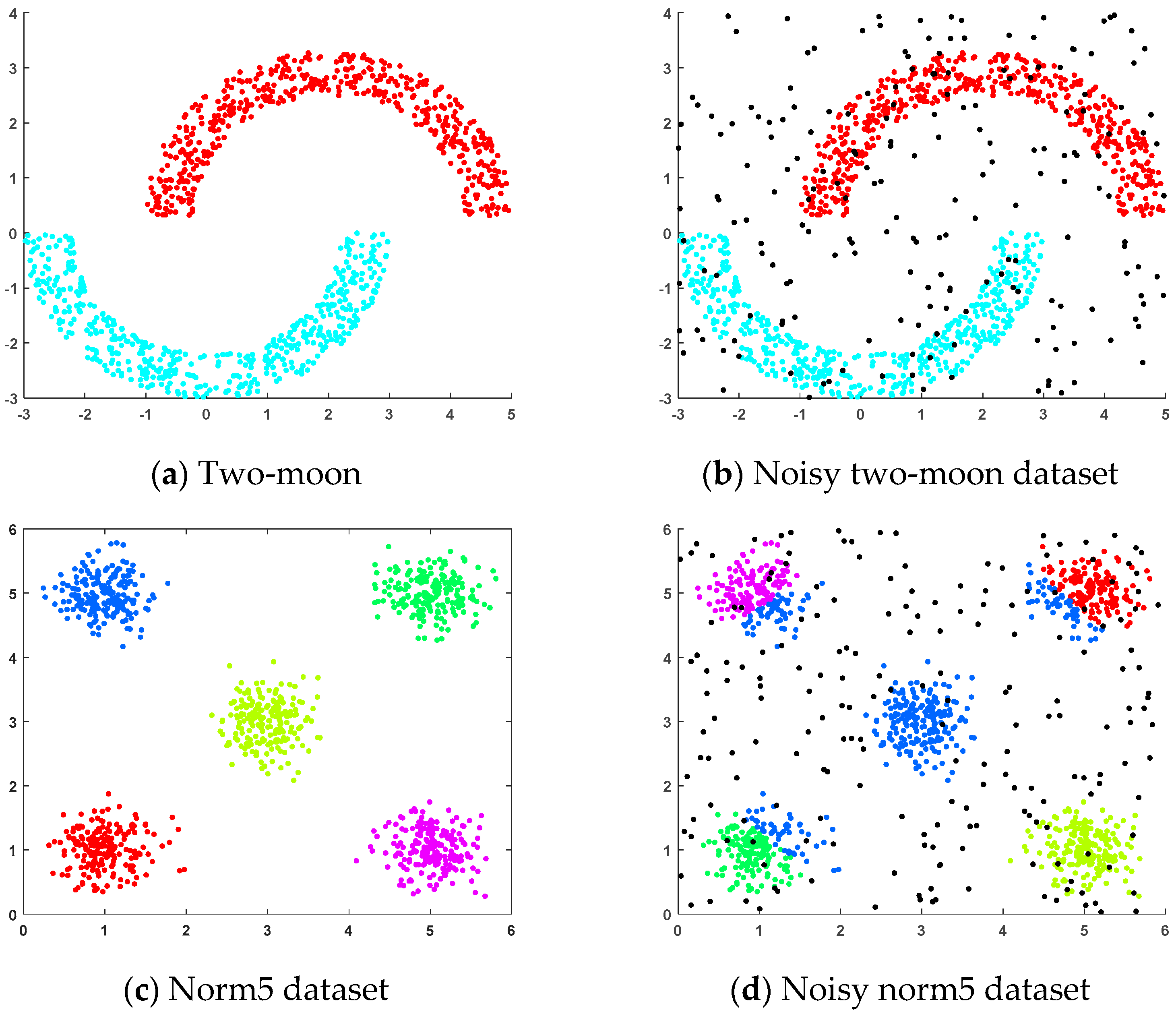
We selected four manually generated datasets to test the clustering performance of FMVSC on artificial datasets:

(a)

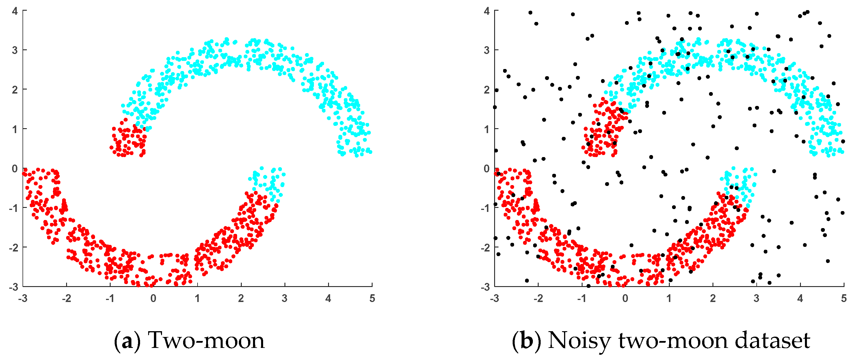
Two-moon dataset: This dataset was generated randomly, where two sets of points were positioned next to each other in a moon shape and each set of points contained 500 random points.

(b)

Noisy two-moon dataset: This dataset was generated by adding 200 randomly generated noise points to the two-moon dataset.

(c)

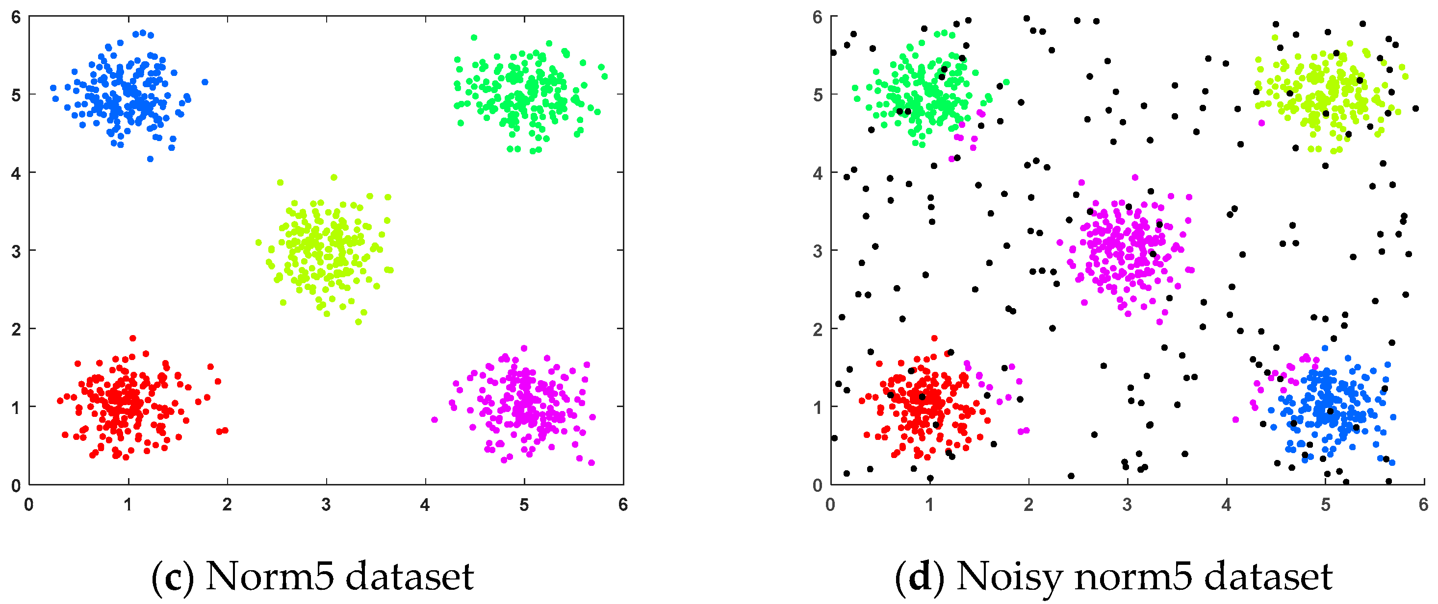
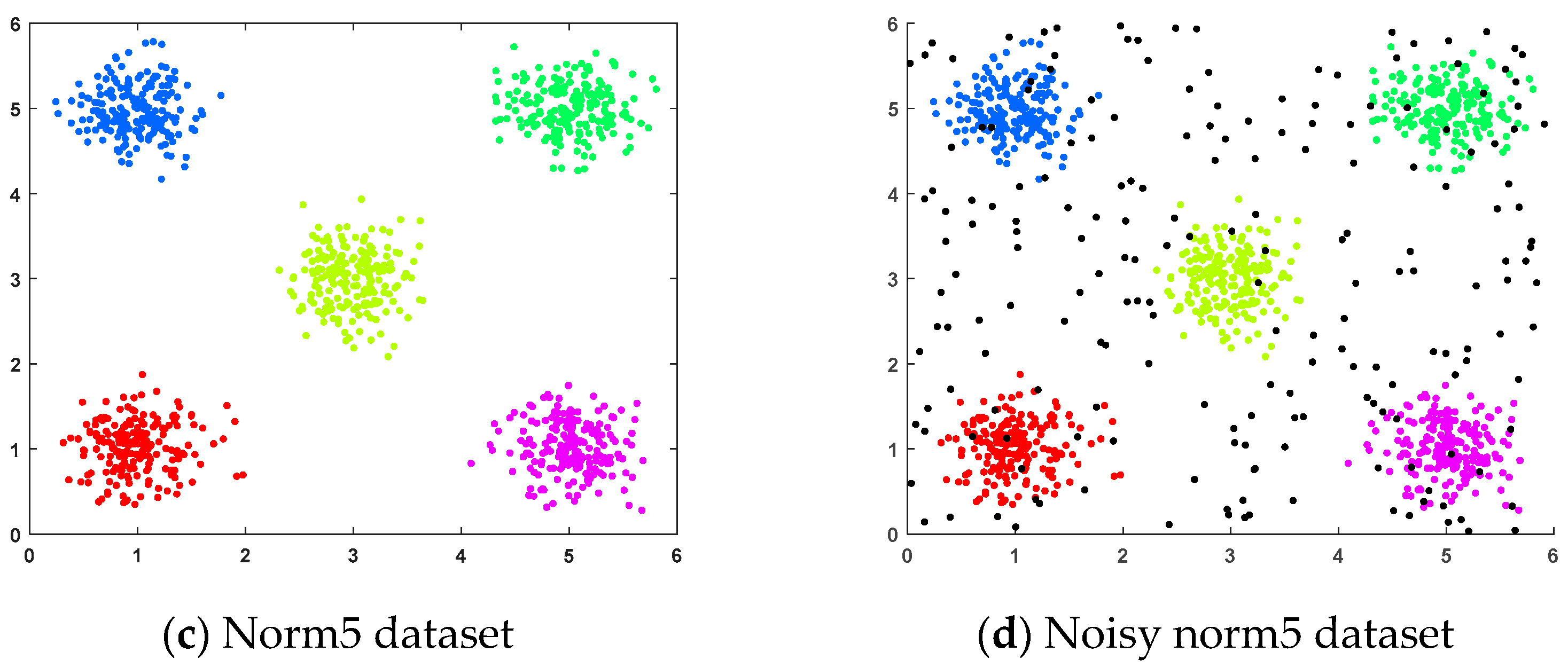
Norm5 dataset: This randomly generated dataset consisted of five clusters, each containing 200 samples, distributed across five spherical regions.

(d)

Noisy norm5 dataset: This dataset was generated by adding 200 randomly generated noise points to the norm5 dataset.

4.1.2. Real-World Datasets

Notting-Hill [40]: This dataset contains 550 facial images in 5 categories, with three views and 110 images in each category.

WebKB [41]: This dataset consists of webpages which are described using contents and links. It has 1051 samples, two classes, and two views.

Wiki [3]: This dataset consists of 2866 images with 10 classes and two views.

CCV [17]: This dataset contains 20 categories extracted from YouTube videos, with 6773 samples and three views.

ALOI [3]: This dataset includes 10,800 images with 100 classes and four views.

Animal [1]: This dataset includes 50 animal species with 11,673 animal images, and it has four features representing four different views.

NUSWIDE [1]: This dataset contains 30,000 images of 31 categories with five views.

YoutubeFace [28]: The face video dataset contains 101,499 images in 31 categories.

More detailed information can be seen in Table 2.

Table 2. Introduction of multi-view datasets.

Dataset	Samples	View	Class	Feature
Notting-Hill	550	3	5	2000, 3304, 6750
WebKB	1051	2	2	1840, 3000
Wiki	2866	2	10	128, 10
CCV	6773	3	20	20, 20, 20
ALOI	10,800	4	100	77, 13, 64, 125
Animal	11,673	4	50	2689, 2000, 2001, 2000
NUSWIDE	30,000	5	31	65, 226, 145, 74, 129
YoutubeFace	101,499	5	31	64, 512, 64, 647, 838

4.2. Compared Methods

To present the performance of the FMVSC method more intuitively, we compared it with eight state-of-the-art methods, which are as follows:

MLRSSC (2018) [18]: This model constructs an affinity matrix with low-rank and sparse constraints.

MSC_IAS (2019) [42]: This model attempts to construct the affinity matrix using the Hilbert–Schmidt independence criterion.

LMVSC (2020) [21]: This model adopts the anchor point strategy to handle large datasets in linear time.

MSGL (2022) [30]: This model attempts to construct an affinity matrix using consensus anchor points and connectivity constraints.

SMVSC (2022) [17]: This model combines anchor graph learning with subspace construction to obtain a clustering indicator matrix.

SFMC (2022) [31]: This model is designed to construct a joint graph in a parameter-free, self-supervised weighted manner.

RAMCSF (2023) [32]: This model attempts to approximate the full sample graph through spectral embedding decomposition.

OMVCDR (2024) [43]: This model addresses large-scale clustering problems through matrix factorization and projection strategies.

4.3. Results on Artificial Datasets

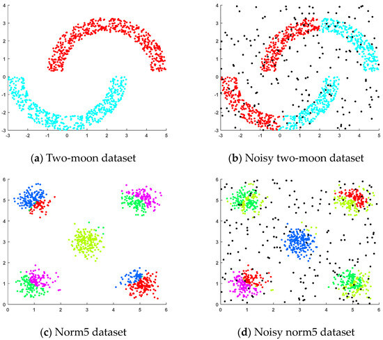
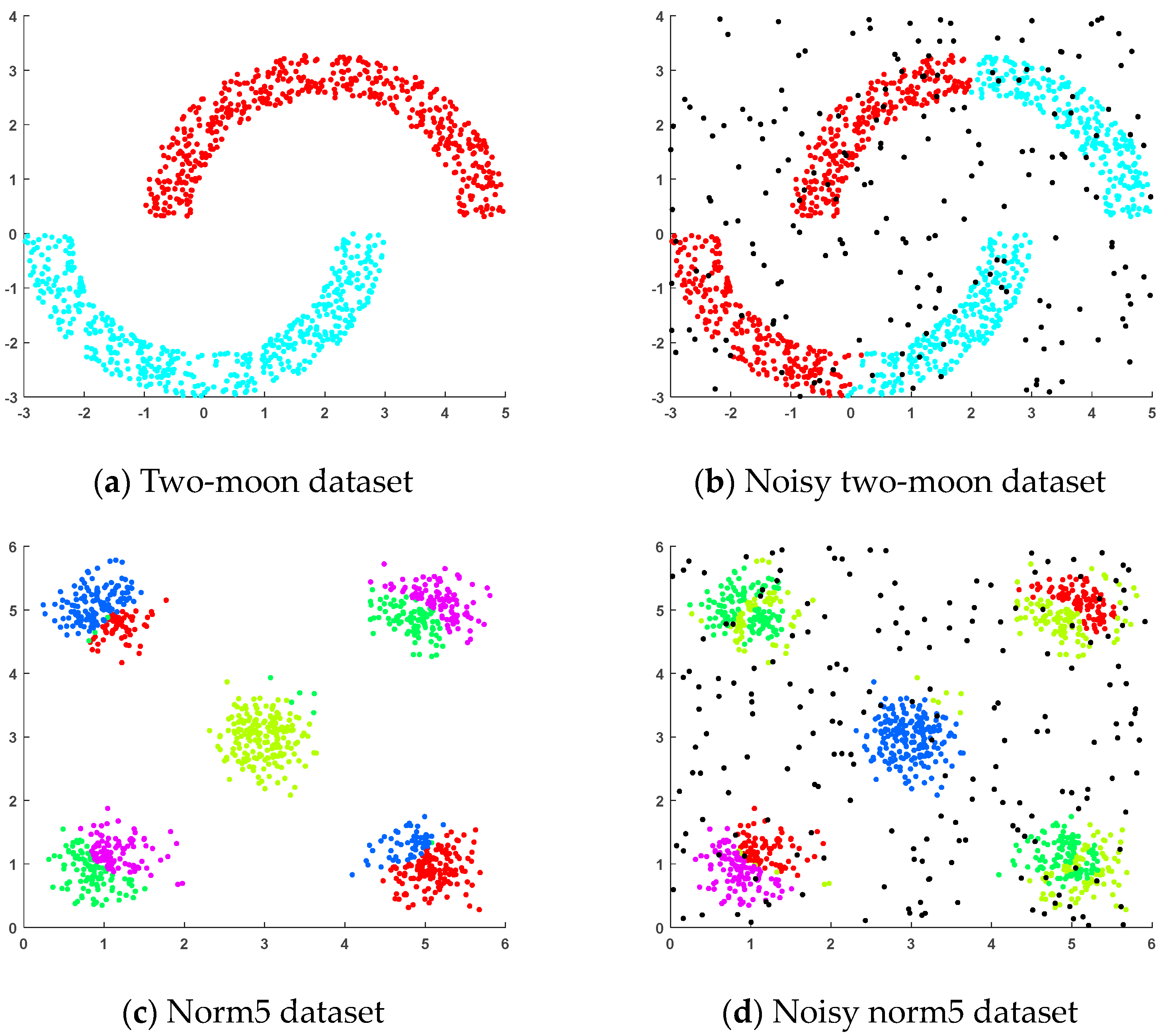
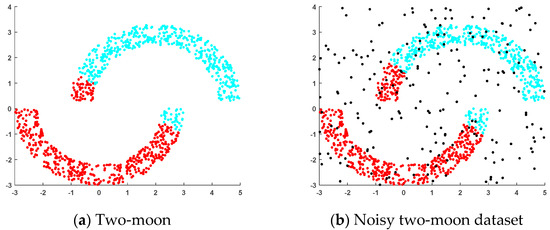
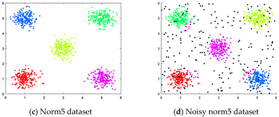
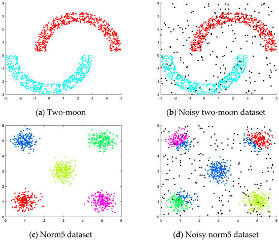
In this section, we explore the performance of FMVSC on artificial datasets. We applied FMVSC and three baseline algorithms to four artificial datasets and visually presented the clustering results in the form of images in Figure 2, Figure 3, Figure 4 and Figure 5, where each color represents a cluster and black points represent noise. It can be observed that MLRSSC failed to correctly distinguish the five clusters in the Norm5 dataset, indicating that MLRSSC performs poorly in multi-cluster scenarios. Additionally, MLRSSC failed to obtain correct clustering results for the Noisy two-moon and Noisy norm5 datasets, demonstrating its lack of robustness and resistance to noise. LMVSC performed poorly on the Two-moon, Noisy two-moon, and Noisy norm datasets, suggesting that LMVSC loses some critical information during the rapid clustering process, leading to poor performance on nonlinear and noisy data. MSGL performed well on the first three datasets but failed to correctly distinguish the Noisy norm dataset, indicating that MSGL lacks robustness and is easily affected by noise. Conversely, FMVSC achieved correct clustering results across all four datasets, demonstrating its strong adaptability to various datasets and superior robustness.

Figure 2. Running results of MLRSSC on artificial datasets.

Figure 3. Running results of LMVSC on artificial datasets.

Figure 4. Running results of MSGL on artificial datasets.

Figure 5. Running results of FMVSC on artificial datasets.

4.4. Experimental Results

We selected four commonly used cluster evaluation metrics, which are as follows:

Accuracy (ACC): ACC measures the proportion of instances which are correctly classified.

Normalized mutual information (NMI): NMI evaluates the degree of similarity between the true and predicted labels.

Purity: Purity assesses how homogenous each cluster is, based on the dominance of a single class within the cluster.

F score: The F score is the harmonic mean of the precision and recall, balancing both metrics.

We conducted extensive experiments on the aforementioned dataset, comparing FMVSC with eight baseline algorithms. The detailed experimental results are shown in Table 3, Table 4, Table 5 and Table 6. The best performance is highlighted in bold black font, while the second-best performance is underlined. “OM” indicates cases where memory limitations occurred. To mitigate the instability caused by randomized methods such as k-means clustering, we selected the optimal parameter settings and repeated the experiments 20 times, reporting the average results and standard deviations. In the experiments, we employed a grid search strategy, where the number of anchor points for each view was explored within the set [k, 3k, 5k] and the hyperparameter $\lambda$ was explored within the set [1, 10, 100, 1000]. Based on the results in Table 3, Table 4, Table 5 and Table 6, the advantages of our method are primarily reflected in the following aspects:

(a)

Compared with other baseline algorithms, FMVSC demonstrated significant superiority in performance. Especially in terms of the ACC metric, FMVSC achieved the optimal value across all cases. Compared with the second-best algorithm, FMVSC improved the ACC scores by 0.44%, 1.4%, 4.9%, 3.1%, 2.5%, 2.1%, 2.0%, and 3.8%, respectively. In the other three metrics, FMVSC also achieved either the optimal or second-best results. This highlights the excellent clustering performance of FMVSC.

(b)

Compared with classic MVSC algorithms such as MLRSSC and MSC_IAS, FMVSC reduced both the time and space complexity. By leveraging a flexible anchor point sampling strategy, it is better suited for large-scale datasets.

(c)

FMVSC also achieved impressive results on smaller-scale datasets. When compared with fast MVSC methods such as LMVSC, MSGL, SMVSC, RAMCSF, and OMVCDR, FMVSC demonstrated clear performance advantages. This indicates that the flexible anchor graphs constructed for each view effectively captured the data space.

(d)

Compared with fast MVSC algorithms such as LMVSC, MSGL, SMVSC, and RAMCSF, the smaller standard deviation of FMVSC’s experimental results indicates that the variation in the results was low, suggesting that FMVSC is stable. Additionally, SFMC and OMVCDR do not rely on randomized methods like k-means clustering during the clustering process, which is why their experimental results had a standard deviation of zero.

Table 3. Accuracy comparison results (mean ± Std).

Dataset	MLRSSC	MSC_IAS	LMVSC	MSGL	SMVSC	SFMC	RAMCSF	OMVCDR	Ours
Year	2018	2019	2020	2022	2022	2022	2023	2024	2024
Notting-Hill	80.61 ± 4.31	77.24 ± 5.46	77.82 ± 6.48	73.41 ± 5.77	75.45 ± 6.33	84.91 ± 0.00	86.64 ± 7.18	83.57 ± 0.00	88.38 ± 4.29
WebKB	90.77 ± 0.22	77.07 ± 1.48	68.34 ± 0.13	93.03 ± 0.00	90.87 ± 0.00	94.76 ± 0.00	94.19 ± 0.00	95.37 ± 0.00	95.81 ± 0.00
Wiki	15.67 ± 0.45	23.97 ± 1.26	49.83 ± 2.33	51.16 ± 1.97	50.03 ± 4.17	33.27 ± 0.00	43.94 ± 2.94	46.71 ± 0.00	56.04 ± 2.14
CCV	15.87 ± 0.31	14.10 ± 0.29	20.12 ± 0.58	15.44 ± 0.41	19.78 ± 0.46	11.13 ± 0.00	14.16 ± 0.87	19.74 ± 0.00	22.87 ± 0.34
ALOI	OM	OM	42.18 ± 1.71	16.93 ± 0.74	52.36 ± 2.24	OM	55.75 ± 2.37	63.84 ± 0.00	66.36 ± 2.11
Animal	OM	OM	10.63 ± 0.19	11.09 ± 0.21	13.16 ± 0.22	OM	15.67 ± 0.42	14.23 ± 0.00	17.77 ± 0.33
NUSWIDE	OM	OM	12.27 ± 0.27	13.60 ± 0.67	12.13 ± 0.37	OM	14.08 ± 0.53	13.53 ± 0.00	16.02 ± 0.39
YoutubeFace	OM	OM	14.25 ± 0.53	16.71 ± 0.57	OM	OM	17.64 ± 0.85	OM	21.39 ± 0.61

The best performance is highlighted in bold black font, while the second-best performance is underlined.

Table 3. Accuracy comparison results (mean ± Std).

Dataset	MLRSSC	MSC_IAS	LMVSC	MSGL	SMVSC	SFMC	RAMCSF	OMVCDR	Ours
Year	2018	2019	2020	2022	2022	2022	2023	2024	2024
Notting-Hill	80.61 ± 4.31	77.24 ± 5.46	77.82 ± 6.48	73.41 ± 5.77	75.45 ± 6.33	84.91 ± 0.00	86.64 ± 7.18	83.57 ± 0.00	88.38 ± 4.29
WebKB	90.77 ± 0.22	77.07 ± 1.48	68.34 ± 0.13	93.03 ± 0.00	90.87 ± 0.00	94.76 ± 0.00	94.19 ± 0.00	95.37 ± 0.00	95.81 ± 0.00
Wiki	15.67 ± 0.45	23.97 ± 1.26	49.83 ± 2.33	51.16 ± 1.97	50.03 ± 4.17	33.27 ± 0.00	43.94 ± 2.94	46.71 ± 0.00	56.04 ± 2.14
CCV	15.87 ± 0.31	14.10 ± 0.29	20.12 ± 0.58	15.44 ± 0.41	19.78 ± 0.46	11.13 ± 0.00	14.16 ± 0.87	19.74 ± 0.00	22.87 ± 0.34
ALOI	OM	OM	42.18 ± 1.71	16.93 ± 0.74	52.36 ± 2.24	OM	55.75 ± 2.37	63.84 ± 0.00	66.36 ± 2.11
Animal	OM	OM	10.63 ± 0.19	11.09 ± 0.21	13.16 ± 0.22	OM	15.67 ± 0.42	14.23 ± 0.00	17.77 ± 0.33
NUSWIDE	OM	OM	12.27 ± 0.27	13.60 ± 0.67	12.13 ± 0.37	OM	14.08 ± 0.53	13.53 ± 0.00	16.02 ± 0.39
YoutubeFace	OM	OM	14.25 ± 0.53	16.71 ± 0.57	OM	OM	17.64 ± 0.85	OM	21.39 ± 0.61

The best performance is highlighted in bold black font, while the second-best performance is underlined.

Table 4. Normalized mutual information comparison results (mean ± Std).

Dataset	MLRSSC	MSC_IAS	LMVSC	MSGL	SMVSC	SFMC	RAMCSF	OMVCDR	Ours
Year	2018	2019	2020	2022	2022	2022	2023	2024	2024
Notting-Hill	67.33 ± 4.09	71.93 ± 3.52	66.33 ± 4.04	59.14 ± 5.81	72.04 ± 4.85	81.62 ± 0.00	77.23 ± 6.47	76.15 ± 0.00	79.86 ± 3.61
WebKB	47.27 ± 0.31	19.09 ± 0.12	13.24 ± 0.08	58.14 ± 0.00	55.19 ± 0.00	62.74 ± 0.00	60.81 ± 0.00	64.29 ± 0.00	73.25 ± 0.00
Wiki	12.31 ± 0.68	18.65 ± 1.03	45.39 ± 2.07	48.63 ± 1.83	46.38 ± 3.25	31.29 ± 0.00	37.62 ± 2.03	41.94 ± 0.00	52.40 ± 1.50
CCV	11.98 ± 0.40	9.50 ± 0.35	16.48 ± 0.47	11.89 ± 0.53	14.82 ± 0.61	3.13 ± 0.00	7.62 ± 0.95	17.58 ± 0.00	19.27 ± 0.41
ALOI	OM	OM	51.23 ± 1.93	22.54 ± 0.81	61.47 ± 1.89	OM	64.73 ± 2.39	72.70 ± 0.00	80.65 ± 1.76
Animal	OM	OM	6.95 ± 0.17	6.47 ± 0.27	12.63 ± 0.24	OM	14.21 ± 0.32	13.29 ± 0.00	14.07 ± 0.24
NUSWIDE	OM	OM	8.13 ± 0.33	1.86 ± 0.60	6.39 ± 0.29	OM	9.27 ± 0.38	13.01 ± 0.00	15.10 ± 0.28
YoutubeFace	OM	OM	5.20 ± 0.37	3.24 ± 0.29	OM	OM	15.19 ± 0.41	OM	17.3 ± 0.43

The best performance is highlighted in bold black font, while the second-best performance is underlined.

Table 4. Normalized mutual information comparison results (mean ± Std).

Dataset	MLRSSC	MSC_IAS	LMVSC	MSGL	SMVSC	SFMC	RAMCSF	OMVCDR	Ours
Year	2018	2019	2020	2022	2022	2022	2023	2024	2024
Notting-Hill	67.33 ± 4.09	71.93 ± 3.52	66.33 ± 4.04	59.14 ± 5.81	72.04 ± 4.85	81.62 ± 0.00	77.23 ± 6.47	76.15 ± 0.00	79.86 ± 3.61
WebKB	47.27 ± 0.31	19.09 ± 0.12	13.24 ± 0.08	58.14 ± 0.00	55.19 ± 0.00	62.74 ± 0.00	60.81 ± 0.00	64.29 ± 0.00	73.25 ± 0.00
Wiki	12.31 ± 0.68	18.65 ± 1.03	45.39 ± 2.07	48.63 ± 1.83	46.38 ± 3.25	31.29 ± 0.00	37.62 ± 2.03	41.94 ± 0.00	52.40 ± 1.50
CCV	11.98 ± 0.40	9.50 ± 0.35	16.48 ± 0.47	11.89 ± 0.53	14.82 ± 0.61	3.13 ± 0.00	7.62 ± 0.95	17.58 ± 0.00	19.27 ± 0.41
ALOI	OM	OM	51.23 ± 1.93	22.54 ± 0.81	61.47 ± 1.89	OM	64.73 ± 2.39	72.70 ± 0.00	80.65 ± 1.76
Animal	OM	OM	6.95 ± 0.17	6.47 ± 0.27	12.63 ± 0.24	OM	14.21 ± 0.32	13.29 ± 0.00	14.07 ± 0.24
NUSWIDE	OM	OM	8.13 ± 0.33	1.86 ± 0.60	6.39 ± 0.29	OM	9.27 ± 0.38	13.01 ± 0.00	15.10 ± 0.28
YoutubeFace	OM	OM	5.20 ± 0.37	3.24 ± 0.29	OM	OM	15.19 ± 0.41	OM	17.3 ± 0.43

The best performance is highlighted in bold black font, while the second-best performance is underlined.

Table 5. Purity comparison results (mean ± Std).

Dataset	MLRSSC	MSC_IAS	LMVSC	MSGL	SMVSC	SFMC	RAMCSF	OMVCDR	Ours
Year	2018	2019	2020	2022	2022	2022	2023	2024	2024
Notting-Hill	81.86+3.84	83.30 ± 4.09	80.59 ± 6.29	79.82 ± 5.33	83.41 ± 5.61	85.45 ± 0.00	86.91 ± 6.63	89.64 ± 0.00	89.14 ± 4.17
WebKB	90.77 ± 0.22	78.12 ± 0.19	68.34 ± 0.13	93.03 ± 0.00	90.87 ± 0.00	94.77 ± 0.00	94.20 ± 0.00	95.37 ± 0.00	95.81 ± 0.00
Wiki	15.37 ± 0.83	23.68 ± 1.27	54.31 ± 2.40	58.33 ± 2.04	51.79 ± 4.59	34.18 ± 0.00	42.36 ± 2.58	47.34 ± 0.00	61.36 ± 2.55
CCV	20.10 ± 0.32	18.25 ± 0.26	23.74 ± 0.43	20.04 ± 0.37	22.25 ± 0.49	11.68 ± 0.00	16.31 ± 0.89	21.36 ± 0.00	24.87 ± 0.33
ALOI	OM	OM	42.32 ± 1.64	22.15 ± 0.77	49.45 ± 2.31	OM	59.86 ± 1.92	64.77 ± 0.00	68.63 ± 1.81
Animal	OM	OM	18.57 ± 0.21	8.84 ± 0.26	14.21 ± 0.21	OM	15.17 ± 0.44	22.06 ± 0.00	21.76 ± 0.30
NUSWIDE	OM	OM	24.32 ± 0.31	25.18 ± 0.51	23.31 ± 0.44	OM	12.53 ± 0.32	23.57 ± 0.00	27.75 ± 0.34
YoutubeFace	OM	OM	27.32 ± 0.25	32.79 ± 0.33	OM	OM	28.64 ± 0.55	OM	31.60 ± 0.38

The best performance is highlighted in bold black font, while the second-best performance is underlined.

Table 5. Purity comparison results (mean ± Std).

Dataset	MLRSSC	MSC_IAS	LMVSC	MSGL	SMVSC	SFMC	RAMCSF	OMVCDR	Ours
Year	2018	2019	2020	2022	2022	2022	2023	2024	2024
Notting-Hill	81.86+3.84	83.30 ± 4.09	80.59 ± 6.29	79.82 ± 5.33	83.41 ± 5.61	85.45 ± 0.00	86.91 ± 6.63	89.64 ± 0.00	89.14 ± 4.17
WebKB	90.77 ± 0.22	78.12 ± 0.19	68.34 ± 0.13	93.03 ± 0.00	90.87 ± 0.00	94.77 ± 0.00	94.20 ± 0.00	95.37 ± 0.00	95.81 ± 0.00
Wiki	15.37 ± 0.83	23.68 ± 1.27	54.31 ± 2.40	58.33 ± 2.04	51.79 ± 4.59	34.18 ± 0.00	42.36 ± 2.58	47.34 ± 0.00	61.36 ± 2.55
CCV	20.10 ± 0.32	18.25 ± 0.26	23.74 ± 0.43	20.04 ± 0.37	22.25 ± 0.49	11.68 ± 0.00	16.31 ± 0.89	21.36 ± 0.00	24.87 ± 0.33
ALOI	OM	OM	42.32 ± 1.64	22.15 ± 0.77	49.45 ± 2.31	OM	59.86 ± 1.92	64.77 ± 0.00	68.63 ± 1.81
Animal	OM	OM	18.57 ± 0.21	8.84 ± 0.26	14.21 ± 0.21	OM	15.17 ± 0.44	22.06 ± 0.00	21.76 ± 0.30
NUSWIDE	OM	OM	24.32 ± 0.31	25.18 ± 0.51	23.31 ± 0.44	OM	12.53 ± 0.32	23.57 ± 0.00	27.75 ± 0.34
YoutubeFace	OM	OM	27.32 ± 0.25	32.79 ± 0.33	OM	OM	28.64 ± 0.55	OM	31.60 ± 0.38

The best performance is highlighted in bold black font, while the second-best performance is underlined.

Table 6. F score comparison results (mean ± Std).

Dataset	MLRSSC	MSC_IAS	LMVSC	MSGL	SMVSC	SFMC	RAMCSF	OMVCDR	Ours
Year	2018	2019	2020	2022	2022	2022	2023	2024	2024
Notting-Hill	71.89 ± 3.77	75.61 ± 4.34	73.24 ± 5.57	77.82 ± 4.14	65.41 ± 5.59	72.45 ± 0.00	78.91 ± 7.09	82.64 ± 0.00	83.74 ± 3.95
WebKB	86.94 ± 0.17	78.39 ± 0.15	62.80 ± 0.11	89.89 ± 0.00	86.58 ± 0.00	92.52 ± 0.00	91.95 ± 0.00	93.56 ± 0.00	93.70 ± 0.00
Wiki	17.46 ± 0.47	25.74 ± 0.74	43.75 ± 2.08	39.77 ± 1.91	37.64 ± 3.41	21.38 ± 0.00	29.72 ± 2.24	31.54 ± 0.00	49.87 ± 2.24
CCV	9.85 ± 0.42	9.22 ± 0.12	11.70 ± 0.31	9.76 ± 0.46	11.93 ± 0.53	10.85 ± 0.00	9.51 ± 0.93	11.78 ± 0.00	13.28 ± 0.27
ALOI	OM	OM	38.43 ± 1.52	10.95 ± 0.74	41.67 ± 1.73	OM	47.82 ± 1.97	53.76 ± 0.00	57.43 ± 1.58
Animal	OM	OM	9.54 ± 0.08	11.18 ± 0.07	10.37 ± 0.15	OM	10.97 ± 0.24	9.27 ± 0.00	10.83 ± 0.16
NUSWIDE	OM	OM	8.84 ± 0.07	10.47 ± 0.43	11.39 ± 0.39	OM	9.33 ± 0.46	10.52 ± 0.00	11.67 ± 0.22
YoutubeFace	OM	OM	10.72 ± 0.19	13.81 ± 0.21	OM	OM	11.31 ± 0.87	OM	14.13 ± 0.35

The best performance is highlighted in bold black font, while the second-best performance is underlined.

Table 6. F score comparison results (mean ± Std).

Dataset	MLRSSC	MSC_IAS	LMVSC	MSGL	SMVSC	SFMC	RAMCSF	OMVCDR	Ours
Year	2018	2019	2020	2022	2022	2022	2023	2024	2024
Notting-Hill	71.89 ± 3.77	75.61 ± 4.34	73.24 ± 5.57	77.82 ± 4.14	65.41 ± 5.59	72.45 ± 0.00	78.91 ± 7.09	82.64 ± 0.00	83.74 ± 3.95
WebKB	86.94 ± 0.17	78.39 ± 0.15	62.80 ± 0.11	89.89 ± 0.00	86.58 ± 0.00	92.52 ± 0.00	91.95 ± 0.00	93.56 ± 0.00	93.70 ± 0.00
Wiki	17.46 ± 0.47	25.74 ± 0.74	43.75 ± 2.08	39.77 ± 1.91	37.64 ± 3.41	21.38 ± 0.00	29.72 ± 2.24	31.54 ± 0.00	49.87 ± 2.24
CCV	9.85 ± 0.42	9.22 ± 0.12	11.70 ± 0.31	9.76 ± 0.46	11.93 ± 0.53	10.85 ± 0.00	9.51 ± 0.93	11.78 ± 0.00	13.28 ± 0.27
ALOI	OM	OM	38.43 ± 1.52	10.95 ± 0.74	41.67 ± 1.73	OM	47.82 ± 1.97	53.76 ± 0.00	57.43 ± 1.58
Animal	OM	OM	9.54 ± 0.08	11.18 ± 0.07	10.37 ± 0.15	OM	10.97 ± 0.24	9.27 ± 0.00	10.83 ± 0.16
NUSWIDE	OM	OM	8.84 ± 0.07	10.47 ± 0.43	11.39 ± 0.39	OM	9.33 ± 0.46	10.52 ± 0.00	11.67 ± 0.22
YoutubeFace	OM	OM	10.72 ± 0.19	13.81 ± 0.21	OM	OM	11.31 ± 0.87	OM	14.13 ± 0.35

The best performance is highlighted in bold black font, while the second-best performance is underlined.

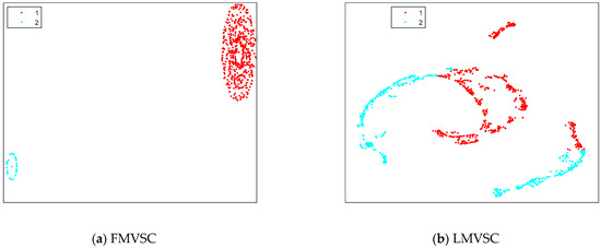
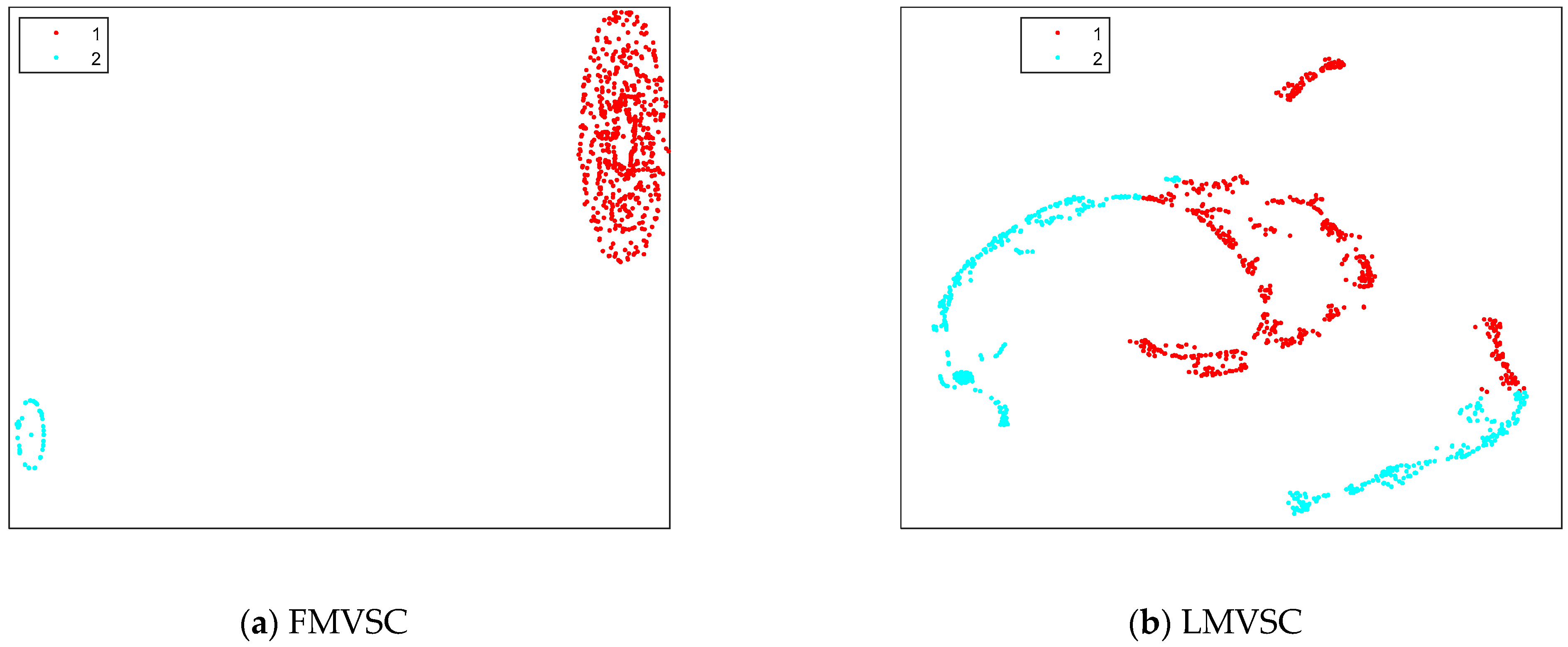
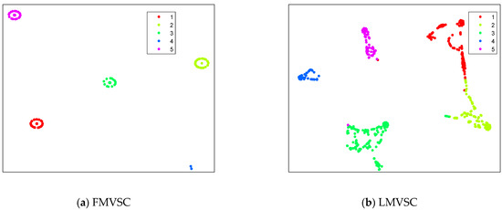
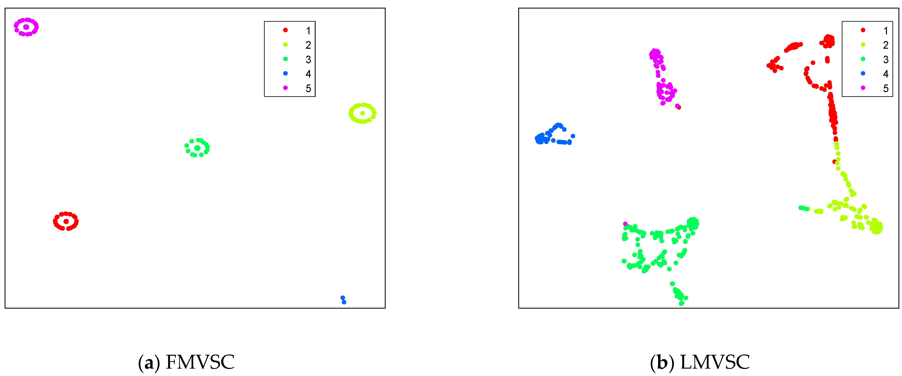
In addition, we applied the t-distributed stochastic neighbor embedding (t-SNE) algorithm to the learned consistent spectral embedding matrices. A commonly used dimensionality reduction technique, t-SNE is primarily used for visualizing high-dimensional data. It works by embedding high-dimensional data into a lower-dimensional space for visualization while preserving the relative distances between data points as much as possible. We selected the WebKB and Notting-Hill datasets for visualization. LMVSC was chosen as the comparison algorithm.

From Figure 6, it can be seen that LMVSC performed poorly on the WebKB dataset, as the distribution of the red and cyan points in its t-SNE plot appears disorganized, with the two clusters not well separated. In contrast, FMVSC performed well, as the red and cyan points are clearly clustered into two distinct regions with a noticeable gap between them, indicating that FMVSC effectively separated the two clusters. Additionally, the red points represent a cluster with 821 samples, while the cyan points represent a cluster with 230 samples. Thus, the red region is noticeably larger than the cyan region.

Figure 6. Illustrations of the learned data distributions of the FMVSC and LMVSC datasets with the t-SNE algorithm on the WebKB database.

From Figure 7, it can be seen that LMVSC did not separate the red and yellow points well, indicating that LMVSC performed poorly in clustering these two clusters. In contrast, FMVSC successfully grouped the five different colored points into their respective regions, demonstrating better clustering performance. Additionally, since each of the five clusters in the Notting-Hill dataset contained 110 sample points, the five different colored regions in FMVSC were almost the same size.

Figure 7. Illustrations of the learned data distribution of FMVSC and LMVSC with the t- SNE algorithm on the Notting-Hill dataset.

These experimental results demonstrate that FMVSC can flexibly construct anchor graphs of varying sizes and integrate consistent spectral embedding matrices which effectively capture the structured information of the data.

Overall, the FMVSC algorithm proposed in this paper showed significant advantages in its clustering results.

4.5. Runtime Comparison

In this section, we recorded the runtimes of each algorithm on the datasets to evaluate the efficiency of FMVSC. Based on Table 7, we can draw the following conclusions:

(a)

FMVSC achieved optimal or near-optimal running efficiency on five datasets, indicating that FMVSC inherits the linear time complexity of the anchor point strategy, significantly reducing the runtime. This is because FMVSC effectively leverages the consensus and complementary information between views, allowing it to converge in fewer iterations. At the same time, our algorithm only requires constructing smaller-sized anchor graphs for each view to represent the current view space.

(b)

Unlike the anchor-based methods, MLRSSC, MSC_IAS, and SFMC construct a representation matrix of $n\times n$ for each view during the clustering process and then combine them into a consistent matrix of $n\times n$. This leads to $O\left(n^2\right)$ for the space complexity and at least $O\left(n^2\right)$ for the time complexity. Therefore, MLRSSC, MSC_IAS, and SFMC may encounter out-of-memory (OM) issues when dealing with large datasets.

(c)

Although LMVSC runs faster on Animal, NUSWIDE, and YoutubeFace, its simple heuristic process does not take full advantage of the consensus and complementary information between views, resulting in poor clustering performance.

Table 7. Runtime comparison (in seconds).

Dataset	MLRSSC	MSC_IAS	LMVSC	MSGL	SMVSC	SFMC	RAMCSF	OMVCDR	Ours
Year	2018	2019	2020	2022	2022	2022	2023	2024	2024
Notting-Hill	25.02	18.78	5.02	18.84	9.04	11.65	2.91	5.82	4.13
WebKB	367.35	120.55	8.62	5.43	7.86	12.58	2.17	4.67	5.36
Wiki	294.33	93.08	7.89	6.20	19.63	35.06	4.21	6.12	3.74
CCV	2352.44	839.46	62.77	35.76	65.86	595.69	23.53	46.87	16.84
ALOI	OM	OM	140.61	203.54	712.91	OM	120.06	241.15	92.42
Animal	OM	OM	230.11	1417.36	903.93	OM	311.27	814.73	444.65
NUSWIDE	OM	OM	367.74	687.33	1684.32	OM	538.09	1725.61	589.64
YoutubeFace	OM	OM	353.93	2134.65	OM	OM	612.30	OM	537.95

The best performance is highlighted in bold black font, while the second-best performance is underlined.

Table 7. Runtime comparison (in seconds).

Dataset	MLRSSC	MSC_IAS	LMVSC	MSGL	SMVSC	SFMC	RAMCSF	OMVCDR	Ours
Year	2018	2019	2020	2022	2022	2022	2023	2024	2024
Notting-Hill	25.02	18.78	5.02	18.84	9.04	11.65	2.91	5.82	4.13
WebKB	367.35	120.55	8.62	5.43	7.86	12.58	2.17	4.67	5.36
Wiki	294.33	93.08	7.89	6.20	19.63	35.06	4.21	6.12	3.74
CCV	2352.44	839.46	62.77	35.76	65.86	595.69	23.53	46.87	16.84
ALOI	OM	OM	140.61	203.54	712.91	OM	120.06	241.15	92.42
Animal	OM	OM	230.11	1417.36	903.93	OM	311.27	814.73	444.65
NUSWIDE	OM	OM	367.74	687.33	1684.32	OM	538.09	1725.61	589.64
YoutubeFace	OM	OM	353.93	2134.65	OM	OM	612.30	OM	537.95

The best performance is highlighted in bold black font, while the second-best performance is underlined.

In summary, both theoretical and experimental results confirm the high efficiency and effectiveness of FMVSC.

4.6. Ablation Experiments

As mentioned earlier, most existing anchor-based multi-view clustering methods use the same number of anchor points for each view. In contrast, our FMVSC method flexibly selects an appropriate number of anchor points for each view. To demonstrate the superiority of FMVSC, we conducted an ablation experiment comparing the equal anchor point strategy with the flexible anchor point strategy. Specifically, the flexible anchor strategy was our proposed FMVSC, and the equal anchor strategy was to replace the anchor selection strategy in FMVSC with a strategy which selected the same number of anchor points per view. As shown in Table 8, the performance of the flexible anchor point strategy was significantly improved, highlighting the advantages of our approach.

Table 8. Ablation experiment of equal number anchors versus our proposed flexible strategy.

Metrics	Anchor Numbers	Datasets
		Notting-Hill	WebKB	Wiki	CCV	ALOI	Animal	NUSWIDE	YoutubeFace
ACC	equal	82.31 ± 3.16	93.26 ± 0.00	51.99 ± 3.06	19.05 ± 0.44	61.09 ± 2.52	14.62 ± 0.36	11.96 ± 0.30	16.11 ± 0.65
	flexible	88.38 ± 4.29	95.81 ± 0.00	56.04 ± 2.14	22.87 ± 0.34	66.36 ± 2.11	17.77 ± 0.33	16.02 ± 0.39	21.39 ± 0.61
NMI	equal	71.64 ± 3.40	69.54 ± 0.00	50.10 ± 1.62	15.11 ± 0.38	76.99 ± 1.94	12.21 ± 0.55	11.83 ± 0.16	12.39 ± 0.29
	flexible	79.86 ± 3.61	73.25 ± 0.00	52.40 ± 1.50	19.27 ± 0.41	80.65 ± 1.76	14.07 ± 0.24	15.10 ± 0.28	18.73 ± 0.43
Purity	equal	83.02 ± 3.18	93.26 ± 0.00	56.74 ± 3.69	22.33 ± 0.39	63.44 ± 2.03	19.15 ± 0.37	23.22 ± 0.23	23.84 ± 0.52
	flexible	89.14 ± 4.17	95.81 ± 0.00	61.36 ± 2.55	24.87 ± 0.33	68.63 ± 1.81	21.76 ± 0.30	27.75 ± 0.34	31.60 ± 0.38
F score	equal	77.64 ± 2.23	90.87 ± 0.00	45.26 ± 3.43	11.13 ± 0.31	51.33 ± 1.47	09.53 ± 0.09	07.92 ± 0.17	10.37 ± 0.24
	flexible	83.74 ± 3.95	93.70 ± 0.00	49.87 ± 2.24	13.28 ± 0.27	57.43 ± 1.58	10.83 ± 0.16	11.67 ± 0.22	14.13 ± 0.35

The bold black font indicates the better result between the two comparisons.

4.7. Parameter Analysis

The hyperparameter $\lambda$ is for fusing various anchor graphs. In this section, we conduct sensitivity analysis experiments on $\lambda$. The specific method involves determining the optimal number of anchors for each view using a grid search strategy, fixing the optimal value, and conducting traversal experiments for $\lambda$ values within the range [1, 10, 50, 100, 200, 500, 1000]. We selected the Notting-Hill, Wiki, CCV, and ALOI datasets to demonstrate the results.

From Figure 8 and Figure 9, it can generally be observed that $\lambda$ has a certain impact on clustering performance when its value is between 1 and 1000, typically being within 0.15. Moreover, we can observe the following based on heuristic experience:

(a)

When $\lambda$ had a small value, such as 1–50, the performance of the ACC, NMI, and Purity datasets was relatively poor. This indicates that when $\lambda$ is too low, the model may lack sufficient regularization or optimization strength, making it difficult to capture the underlying structure of the data.

(b)

As $\lambda$ increased to a moderate range, such as 100–200, all indicators reached their peak performance. This suggests that at this range, the value of $\lambda$ balanced the optimization of model performance with the prevention of overfitting.

(c)

When $\lambda$ became excessively large, such as 500–1000, the performance of all indicators began to slightly decline. This indicates that excessive regularization may limit the model’s clustering capability, resulting in reduced performance.

Figure 8. The sensitivity analysis experiments of hyperparameter λ on the Notting-Hill and Wiki datasets.

Figure 8. The sensitivity analysis experiments of hyperparameter λ on the Notting-Hill and Wiki datasets.

Figure 9. The sensitivity analysis experiments of hyperparameter λ on the CCV and ALOI datasets.

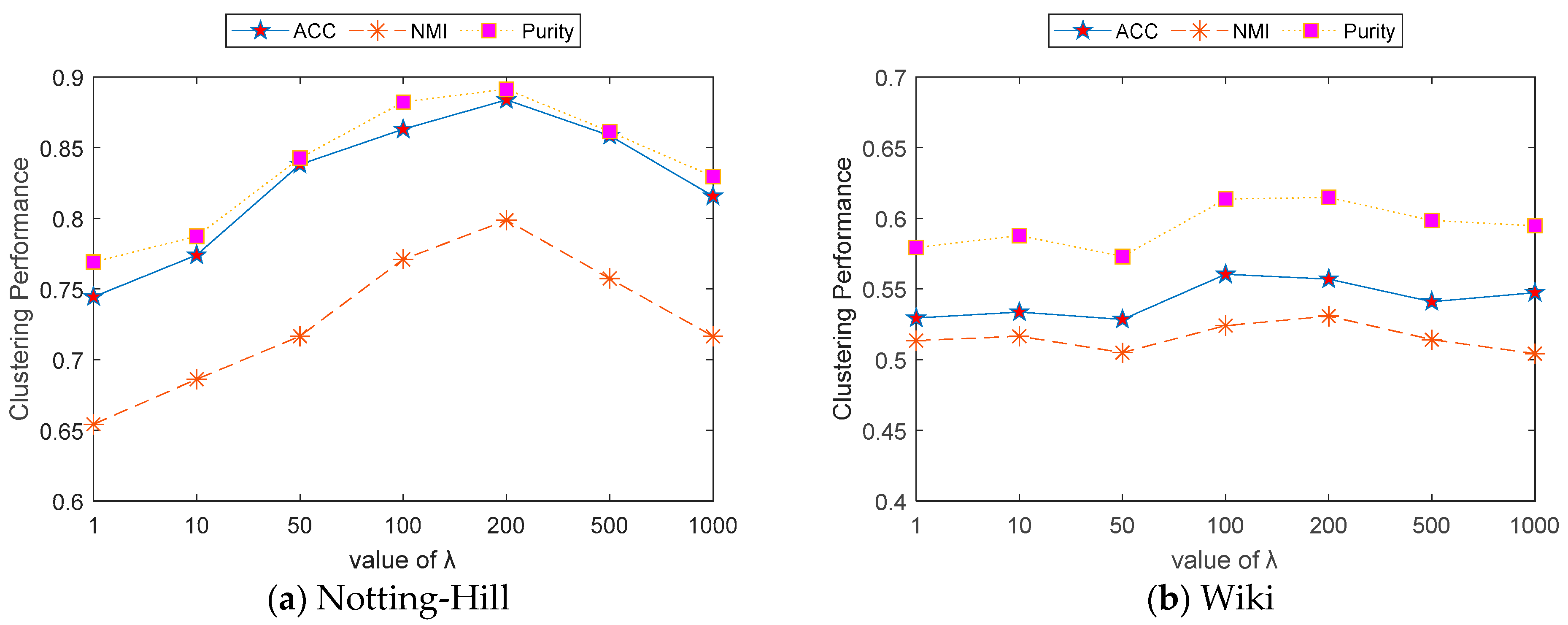
Figure 9. The sensitivity analysis experiments of hyperparameter λ on the CCV and ALOI datasets.

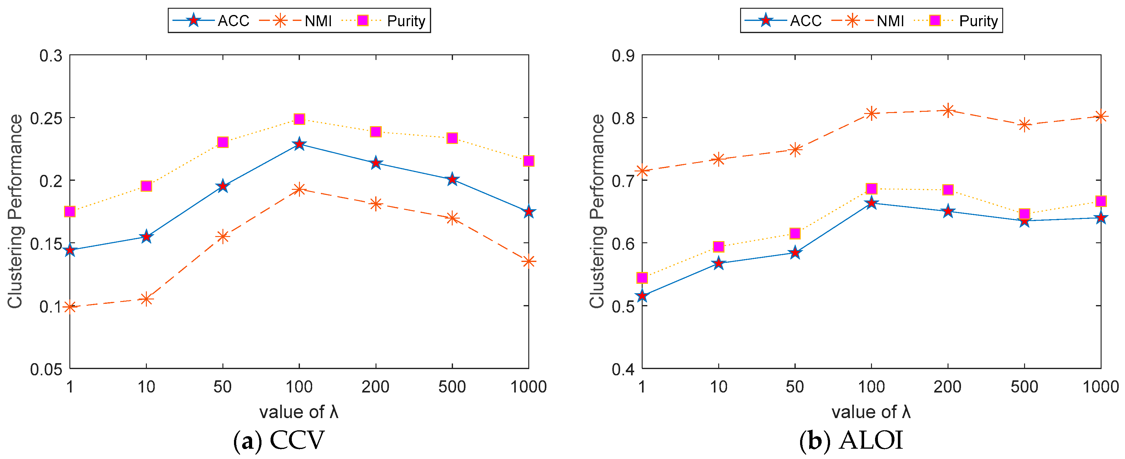
In summary, when $\lambda$ was set within the range of 100–200, FMVSC could effectively capture the latent structure among the data and achieve optimal clustering performance.

4.8. Convergence Analysis

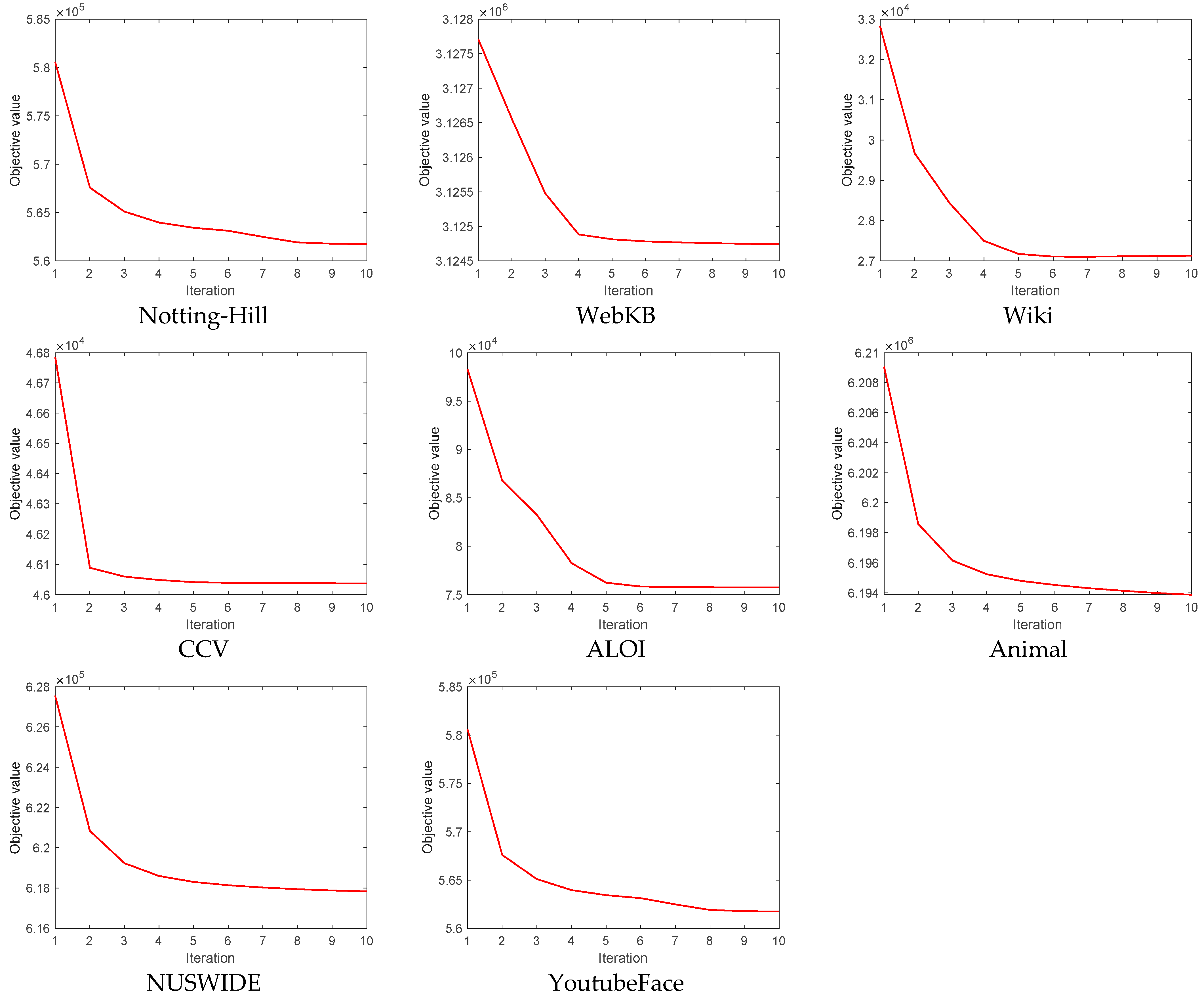
To prove that FMVSC is a convergence algorithm, we carried out the convergence analysis proof in Section 3. Here, we will continue to prove the convergence of FMVSC experimentally. As shown in Figure 10, the horizontal coordinate is the number of iterations of the experiment, and the vertical coordinate is the function value of our objective function. The trend of the objective value decreasing is evident. In all of the plots, the objective value decreased rapidly in the first few iterations, and as the number of iterations increased, the rate of decrease gradually slowed down. This indicates that the algorithm converged quickly in the initial stages of optimization, while progress slowed down in the later stages. Specially, we can make the following observations:

(a)

There were differences in the convergence speeds across different datasets. The objective values of some datasets, like WebKB, Wiki, CCV, and ALOI, nearly reached convergence within the first five iterations, indicating that FMVSC can quickly find a good solution on these datasets. On the other hand, the objective values of datasets like Notting-Hill, Animal, NUSWIDE, and YoutubeFace required more iterations to reach convergence, indicating that the convergence process was more complex for these datasets, and more computation time was needed.

(b)

The objective values for all datasets stabilized after 10 iterations, indicating that our algorithm can reach a convergent state after only a few iterations across different datasets. This makes FMVSC particularly suitable for large-scale datasets.

Figure 10. The convergence graph of the objective function for each dataset.

Figure 10. The convergence graph of the objective function for each dataset.

In summary, we proved the convergence of FMVSC theoretically and experimentally.

5. Conclusions

In this paper, we proposed a scalable and fast multi-view subspace clustering method based on flexible anchor fusion. Different from the existing anchor-point based method, the same number of anchor points was selected from each view, and then the fusion map was obtained by a simple linear weighted combination. Our proposed framework can automatically select the number of anchor points suitable for each data space view and then flexibly integrate anchor graphs with different sizes. Our framework also learns the global and local information between data, which allows our fusion graph to preserve the clustering structure between views to the maximum extent possible. In order to solve our proposed objective function, we proposed an optimization algorithm which can prove convergence both experimentally and theoretically. Through a large number of experiments, we can also see that the clustering accuracy and efficiency of our proposed algorithm were better than the current large-scale multi-view clustering methods. Of course, FMVSC also has some limitations. For example, we have not yet extended it to the field of incomplete multi-view clustering. In future research, we will focus on applying the flexible anchor graph fusion strategy to incomplete multi-view clustering.

References

- Zhou, S.; Yang, M.; Wang, X.; Song, W. Anchor-based scalable multi-view subspace clustering. Inf. Sci. 2024, 666, 120374. [Google Scholar] [CrossRef] [Scilit]
- Wang, S.; Liu, X.; Zhu, X.; Zhang, P.; Zhang, Y.; Gao, F.; Zhu, E. Fast parameter-free multi-view subspace clustering with consensus anchor guidance. IEEE Trans. Image Process. 2021, 31, 556–568. [Google Scholar] [CrossRef] [Scilit] [PubMed]
- Wang, S.; Liu, X.; Liu, S.; Tu, W.; Zhu, E. Scalable and structural multi-view graph clustering with adaptive anchor fusion. IEEE Trans. Image Process. 2024, 33, 4627–4639. [Google Scholar] [CrossRef] [Scilit]
- Peng, X.; Zhu, H.; Feng, J.; Shen, C.; Zhang, H.; Zhou, J.T. Deep clustering with sample-assignment invariance prior. IEEE Trans. Neural Netw. Learn. Syst. 2019, 31, 4857–4868. [Google Scholar] [CrossRef] [Scilit]
- Wang, Q.; Qin, Z.; Nie, F.; Li, X. Spectral embedded adaptive neighbors clustering. IEEE Trans. Neural Netw. Learn. Syst. 2018, 30, 1265–1271. [Google Scholar] [CrossRef] [Scilit]
- Yang, G.; Li, Q.; Yun, Y.; Lei, Y.; You, J. Hypergraph Learning-Based Semi-Supervised Multi-View Spectral Clustering. Electronics 2023, 12, 4083. [Google Scholar] [CrossRef] [Scilit]
- Xie, D.; Li, Z.; Sun, Y.; Song, W. Robust Tensor Learning for Multi-View Spectral Clustering. Electronics 2024, 13, 2181. [Google Scholar] [CrossRef] [Scilit]
- Chen, J.; Yi, Z. Sparse representation for face recognition by discriminative low-rank matrix recovery. J. Vis. Commun. Image Represent. 2014, 25, 763–773. [Google Scholar] [CrossRef] [Scilit]
- Liu, M.; Liang, K.; Zhao, Y.; Tu, W.; Zhou, S.; Gan, X.; Liu, X.; He, K. Self-supervised temporal graph learning with temporal and structural intensity alignment. IEEE Trans. Neural Netw. Learn. Syst. 2024, 1–13. [Google Scholar] [CrossRef] [Scilit] [PubMed]
- Wan, X.; Liu, J.; Liang, W.; Liu, X.; Wen, Y.; Zhu, E. Continual multi-view clustering. In Proceedings of the 30th ACM International Conference on Multimedia, Lisboa, Portugal, 10–14 October 2022; pp. 3676–3684. [Google Scholar]
- Gao, H.; Nie, F.; Li, X.; Huang, H. Multi-view subspace clustering. In Proceedings of the IEEE International Conference on Computer Vision, Santiago, Chile, 13–16 December 2015; pp. 4238–4246. [Google Scholar]
- Lan, M.; Meng, M.; Yu, J.; Wu, J. Generalized multi-view collaborative subspace clustering. IEEE Trans. Circuits Syst. Video Technol. 2021, 32, 3561–3574. [Google Scholar] [CrossRef] [Scilit]
- Chen, Y.; Xiao, X.; Peng, C.; Lu, G.; Zhou, Y. Low-rank tensor graph learning for multi-view subspace clustering. IEEE Trans. Circuits Syst. Video Technol. 2021, 32, 92–104. [Google Scholar] [CrossRef] [Scilit]
- Wang, S.; Wang, Y.; Lu, G.; Le, W. Mixed structure low-rank representation for multi-view subspace clustering. Appl. Intell. 2023, 53, 18470–18487. [Google Scholar] [CrossRef] [Scilit]
- Lan, W.; Yang, T.; Chen, Q.; Zhang, S.; Dong, Y.; Zhou, H.; Pan, Y. Multiview subspace clustering via low-rank symmetric affinity graph. IEEE Trans. Neural Netw. Learn. Syst. 2023, 35, 11382–11395. [Google Scholar] [CrossRef] [Scilit]
- Ma, H.; Wang, S.; Zhang, J.; Yu, S.; Liu, S.; Liu, X.; He, K. Symmetric Multi-view Subspace Clustering with Automatic Neighbor Discovery. IEEE Trans. Circuits Syst. Video Technol. 2024, 34, 8766–8778. [Google Scholar] [CrossRef] [Scilit]
- Sun, M.; Zhang, P.; Wang, S.; Zhou, S.; Tu, W.; Liu, X.; Zhu, E.; Wang, C. Scalable multi-view subspace clustering with unified anchors. In Proceedings of the 29th ACM International Conference on Multimedia, Virtual Event, China, 20–24 October 2021; pp. 3528–3536. [Google Scholar]
- Brbić, M.; Kopriva, I. Multi-view low-rank sparse subspace clustering. Pattern Recognit. 2018, 73, 247–258. [Google Scholar] [CrossRef] [Scilit]
- Lu, C.; Feng, J.; Lin, Z.; Mei, T.; Yan, S. Subspace clustering by block diagonal representation. IEEE Trans. Pattern Anal. Mach. Intell. 2018, 41, 487–501. [Google Scholar] [CrossRef] [Scilit]
- Chen, X.; Cai, D. Large scale spectral clustering with landmark-based representation. In Proceedings of the AAAI Conference on Artificial Intelligence, San Francisco, CA, USA, 7–11 August 2011; pp. 313–318. [Google Scholar]
- Kang, Z.; Zhou, W.; Zhao, Z.; Shao, J.; Han, M.; Xu, Z. Large-scale multi-view subspace clustering in linear time. In Proceedings of the AAAI Conference on Artificial Intelligence, New York, NY, USA, 7–12 February 2020; pp. 4412–4419. [Google Scholar]
- Li, Y.; Nie, F.; Huang, H.; Huang, J. Large-scale multi-view spectral clustering via bipartite graph. In Proceedings of the AAAI Conference on Artificial Intelligence, Austin, TX, USA, 25–30 January 2015. [Google Scholar]
- Liu, S.; Wang, S.; Zhang, P.; Xu, K.; Liu, X.; Zhang, C.; Gao, F. Efficient one-pass multi-view subspace clustering with consensus anchors. In Proceedings of the AAAI Conference on Artificial Intelligence, Vancouver, BC, Canada, 27 February–2 March 2022; pp. 7576–7584. [Google Scholar]
- Chen, J.; Yang, J. Robust subspace segmentation via low-rank representation. IEEE Trans. Cybern. 2013, 44, 1432–1445. [Google Scholar] [CrossRef] [Scilit]
- Elhamifar, E.; Vidal, R. Sparse subspace clustering: Algorithm, theory, and applications. IEEE Trans. Pattern Anal. Mach. Intell. 2013, 35, 2765–2781. [Google Scholar] [CrossRef] [Scilit]
- Nie, F.; Chang, W.; Wang, R.; Li, X. Learning an optimal bipartite graph for subspace clustering via constrained Laplacian rank. IEEE Trans. Cybern. 2021, 53, 1235–1247. [Google Scholar] [CrossRef] [Scilit]
- Parsons, L.; Haque, E.; Liu, H. Subspace clustering for high dimensional data: A review. ACM Sigkdd Explor. Newsl. 2004, 6, 90–105. [Google Scholar] [CrossRef] [Scilit]
- Zhou, S.; Wang, X.; Yang, M.; Song, W. Multi-view clustering with adaptive anchor and bipartite graph learning. Neurocomputing 2025, 611, 128627. [Google Scholar] [CrossRef] [Scilit]
- Shi, L.; Cao, L.; Wang, J.; Chen, B. Enhanced latent multi-view subspace clustering. IEEE Trans. Circuits Syst. Video Technol. 2024, 34, 12480–12495. [Google Scholar] [CrossRef] [Scilit]
- Kang, Z.; Lin, Z.; Zhu, X.; Xu, W. Structured graph learning for scalable subspace clustering: From single view to multiview. IEEE Trans. Cybern. 2021, 52, 8976–8986. [Google Scholar] [CrossRef] [Scilit] [PubMed]
- Li, X.; Zhang, H.; Wang, R.; Nie, F. Multiview clustering: A scalable and parameter-free bipartite graph fusion method. IEEE Trans. Pattern Anal. Mach. Intell. 2020, 44, 330–344. [Google Scholar] [CrossRef] [Scilit]
- Yang, B.; Wu, J.; Zhang, X.; Lin, Z.; Nie, F.; Chen, B. Robust anchor-based multi-view clustering via spectral embedded concept factorization. Neurocomputing 2023, 528, 136–147. [Google Scholar] [CrossRef] [Scilit]
- Lao, J.; Huang, D.; Wang, C.-D.; Lai, J.-H. Towards scalable multi-view clustering via joint learning of many bipartite graphs. IEEE Trans. Big Data 2023, 10, 77–91. [Google Scholar] [CrossRef] [Scilit]
- Chan, P.K.; Schlag, M.D.; Zien, J.Y. Spectral k-way ratio-cut partitioning and clustering. In Proceedings of the 30th international Design Automation Conference, Dallas, TX, USA, 14–18 June 1993; pp. 749–754. [Google Scholar]
- Li, L.; He, H. Bipartite graph based multi-view clustering. IEEE Trans. Knowl. Data Eng. 2020, 34, 3111–3125. [Google Scholar] [CrossRef] [Scilit]
- Jiang, T.; Gao, Q.; Gao, X. Multiple graph learning for scalable multi-view clustering. arXiv 2021, arXiv:2106.15382. [Google Scholar]
- Wang, W.; Carreira-Perpinán, M.A. Projection onto the probability simplex: An efficient algorithm with a simple proof, and an application. arXiv 2013, arXiv:1309.1541. [Google Scholar]
- Wang, S.; Liu, X.; Zhu, E.; Tang, C.; Liu, J.; Hu, J.; Xia, J.; Yin, J. Multi-view clustering via late fusion alignment maximization. In Proceedings of the IJCAI, Macao, China, 10–16 August 2019; pp. 3778–3784. [Google Scholar]
- Bezdek, J.C.; Hathaway, R.J. Convergence of alternating optimization. Neural Parallel Sci. Comput. 2003, 11, 351–368. [Google Scholar]
- Zhang, Y.-F.; Xu, C.; Lu, H.; Huang, Y.-M. Character identification in feature-length films using global face-name matching. IEEE Trans. Multimed. 2009, 11, 1276–1288. [Google Scholar] [CrossRef] [Scilit]
- Cai, D.; He, X.; Wu, X.; Han, J. Non-negative matrix factorization on manifold. In Proceedings of the 2008 Eighth IEEE International Conference on Data Mining, Pisa, Italy, 15–19 December 2008; pp. 63–72. [Google Scholar]
- Wang, X.; Lei, Z.; Guo, X.; Zhang, C.; Shi, H.; Li, S.Z. Multi-view subspace clustering with intactness-aware similarity. Pattern Recognit. 2019, 88, 50–63. [Google Scholar] [CrossRef] [Scilit]
- Wan, X.; Liu, J.; Gan, X.; Liu, X.; Wang, S.; Wen, Y.; Wan, T.; Zhu, E. One-step multi-view clustering with diverse representation. IEEE Trans. Neural Netw. Learn. Syst. 2024, 1–13. [Google Scholar] [CrossRef] [Scilit] [PubMed]
Disclaimer/Publisher’s Note: The statements, opinions and data contained in all publications are solely those of the individual author(s) and contributor(s) and not of MDPI and/or the editor(s). MDPI and/or the editor(s) disclaim responsibility for any injury to people or property resulting from any ideas, methods, instructions or products referred to in the content. |
© 2025 by the authors. Licensee MDPI, Basel, Switzerland. This article is an open access article distributed under the terms and conditions of the Creative Commons Attribution (CC BY) license (https://creativecommons.org/licenses/by/4.0/).