1. Introduction
HVDC transmission systems occupy a core position in energy transmission and distribution due to their large transmission capacity and long transmission distance advantages. Especially in the rapid development of new energy sources, the demand for cross-regional transmission of clean energy is increasing, further highlighting the importance of HVDC transmission projects. However, with the enhancement of system complexity and the diversification of operating environments, the risk of faults in HVDC transmission systems has also risen. Among these, high-resistance grounding faults, a common type of grounding fault in HVDC transmission systems, severely impact protective actions and pose significant threats to transmission lines. Accurate localization of such faults is crucial for ensuring system safety and reliability of power supply [
1].
Currently, the traveling wave-based fault location method is widely used in engineering for fault localization. However, the accuracy of this method relies on the precise identification of the wavefronts of the reflected wave and the initial traveling wave, as well as the accurate selection of the traveling wave velocity [
2]. When the fault resistance is very large, and the traveling wave is too weak to detect, it is difficult to determine the surge arrival time. The traditional fault distance calculated using the traveling wave method is based on the surge traveling time and wave velocity [
3]. Therefore, in the case of high-resistance grounding faults, the traditional traveling wave-based fault location method often struggles to provide accurate localization. Furthermore, other existing fault location methods, such as the natural frequency method, although they do not require the identification of the initial wavefront of the fault, still rely on the accurate extraction of fault frequencies and the correct selection of waveforms to maintain localization accuracy. Meanwhile, fault analysis methods depend on the precise acquisition and calculation of line parameters and are greatly influenced by parameter changes [
4].
In recent years, deep learning technology has provided new avenues for fault locations in HVDC transmission systems. Deep learning-based fault location methods rely on fault waveform training to achieve fault localization, with less dependence on accurate mathematical models and less influence from transition resistance, system operating modes, and fault types. Cui et al. [
5] extract fault voltage and current signals, process them using Singular Value Decomposition (SVD), and then use a Generalized Regression Neural Network (GRNN) for fault location. Johnson et al. [
6] employ Support Vector Machines (SVM) to perform fault location and fault type discrimination on HVDC transmission lines using single-ended voltage and current waveforms. However, neither of these studies verifies the effectiveness of the proposed methods in scenarios with high transition resistance grounding faults or when fault signals are noisy. Lan et al. [
7] propose a double-ended fault location model based on a One-Dimensional Convolutional Neural Network (1D-CNN). Compared to traditional double-ended traveling wave-based fault location methods, it does not require precise time synchronization. It overcomes the difficulties in determining the traveling wave velocity and identifying wavefronts during high-resistance grounding faults. However, it does not consider the scenario when the signal sampling frequency of actual equipment is low. Wang et al. [
8] establish a Convolutional Neural Network-Long Short-Term Memory (CNN-LSTM) single-ended HVDC transmission system fault location model and study the impact of signal sampling frequency on the accuracy of the fault location model. It also demonstrates that this method relies on a higher signal sampling frequency to ensure high localization accuracy.
With the continuous emergence of various innovative deep learning network structures, the Residual Neural Network (ResNet) has achieved successful applications in electrical domains such as short-term load forecasting [
9], motor fault diagnosis [
10], and dynamic planning of transmission networks [
11], thanks to its unique residual learning mechanism and efficient feature transfer capabilities. As a further improvement of ResNet, the DRSN significantly enhances the model’s robustness to noisy data and the accuracy of feature extraction by incorporating mechanisms such as soft thresholding into the network. This characteristic gives the DRSN unique advantages in multiple applications in the electrical field. Zhang et al. [
12] successfully apply the DRSN to voiceprint recognition in the power industry, effectively demonstrating its ability to distinguish and suppress noise features in complex and noisy electronic environments, significantly improving the accuracy of voiceprint recognition. Zhang et al. [
13] extend the innovative advantages of DRSN to photovoltaic Direct Current (DC) arc fault detection, leveraging its powerful feature extraction capabilities to precisely capture subtle fault features, providing strong support for the safe operation and maintenance of photovoltaic systems. Wang et al. [
14] combine the DRSN structure with the Temporal Convolutional Network (TCN) for photovoltaic power prediction, achieving enhanced prediction of photovoltaic power generation output with only a minimal increase in parameters. However, the DRSN has not yet been applied in the fault location field in HVDC transmission systems.
Most research on fault location methods for HVDC transmission systems has hitherto predominantly focused on grounding scenarios involving transition resistances less than 500 Ω. However, in the practical operations of HVDC transmission systems, high transition resistance grounding faults are more prevalent, with transition resistance values potentially reaching several kilohms. Furthermore, taking into account the sampling frequency limitations of actual equipment, as stipulated by the international standard IEC-61869-9 [
15], the maximum allowable sampling frequency for DC substations is 96 kHz, while the highest sampling frequency in typical DC projects is 10 kHz [
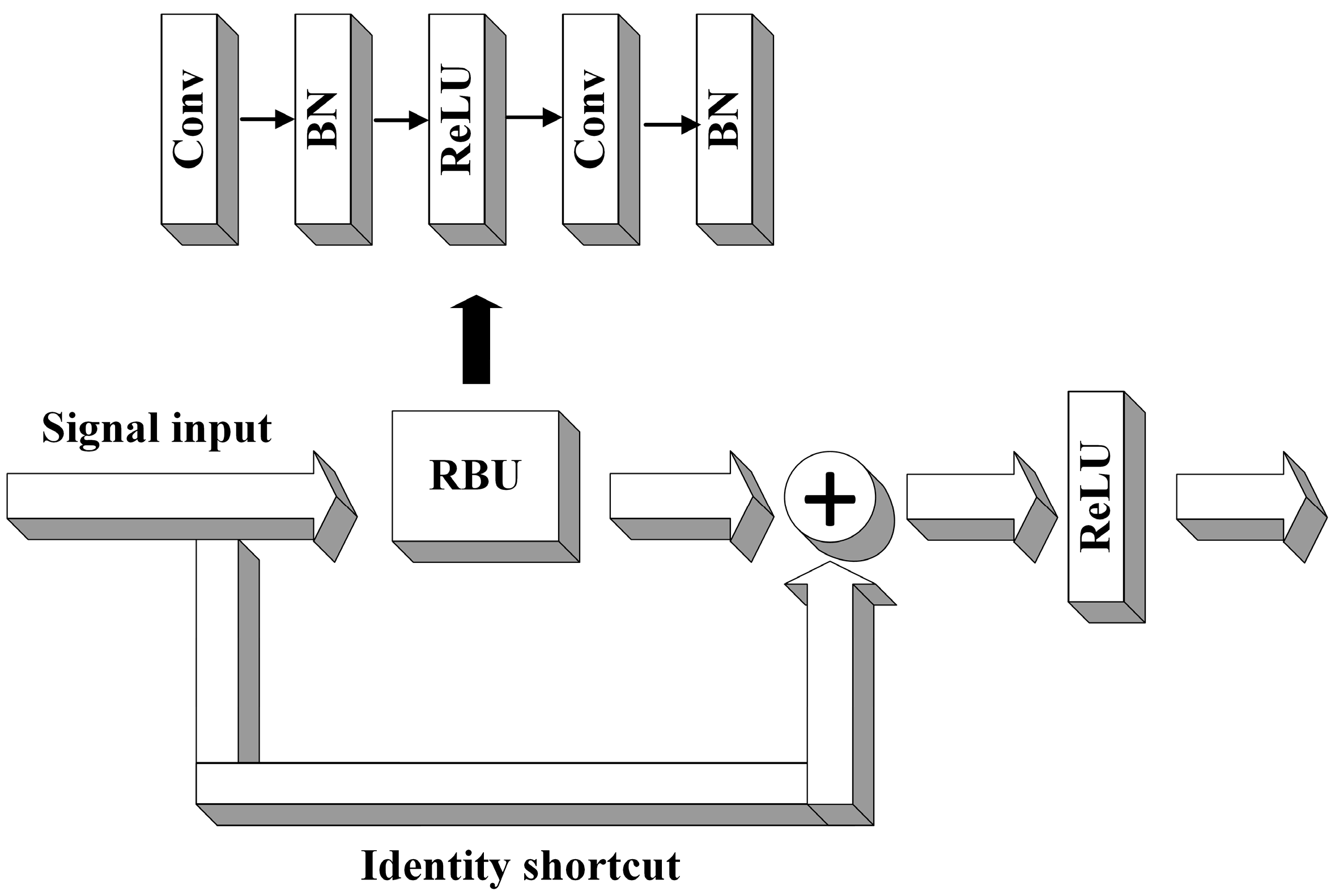
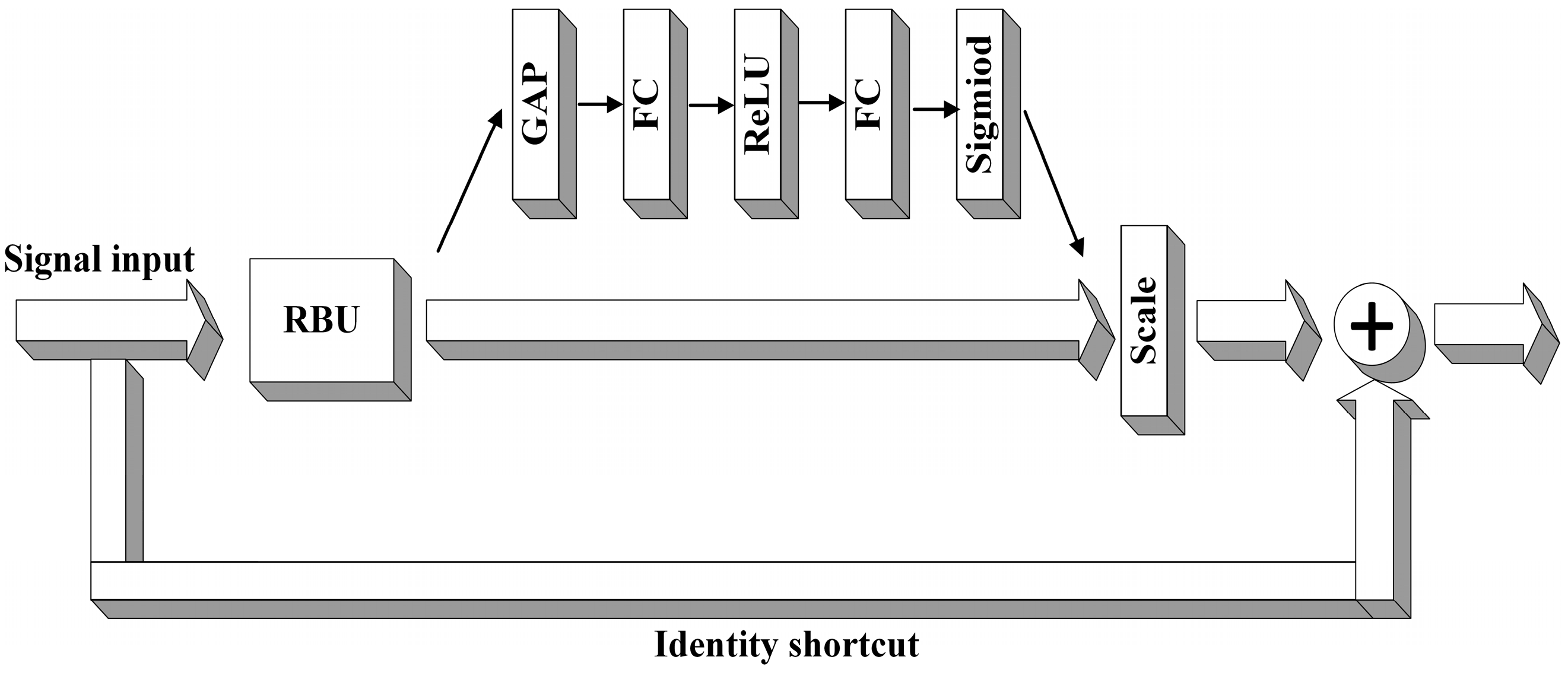
16]. Additionally, in real-world engineering applications, fault data may be influenced by noise and redundant information stemming from equipment limitations and corona discharge, which can impact fault location accuracy. Therefore, this article proposes a high-resistance grounding fault location method for HVDC transmission systems based on the DRSN. This method targets explicitly high transition resistance grounding fault scenarios, considering the precision limitations of equipment sampling frequencies in practical engineering environments and the prevalent noise interference in fault data. The proposed approach utilizes VMD as feature engineering to perform modal decomposition on fault signals, effectively extracting fault signal features. Subsequently, the residual structure of the DRSN is employed to reduce feature loss during data transmission, enhance the model’s feature extraction capabilities when dealing with data with fewer signal points, and address issues of gradient vanishing and model degradation. Simultaneously, by introducing attention mechanisms and soft thresholding operations, the model can eliminate redundant features and enhance the discriminability of high-level features [
17]. The main contributions of this article are as follows:
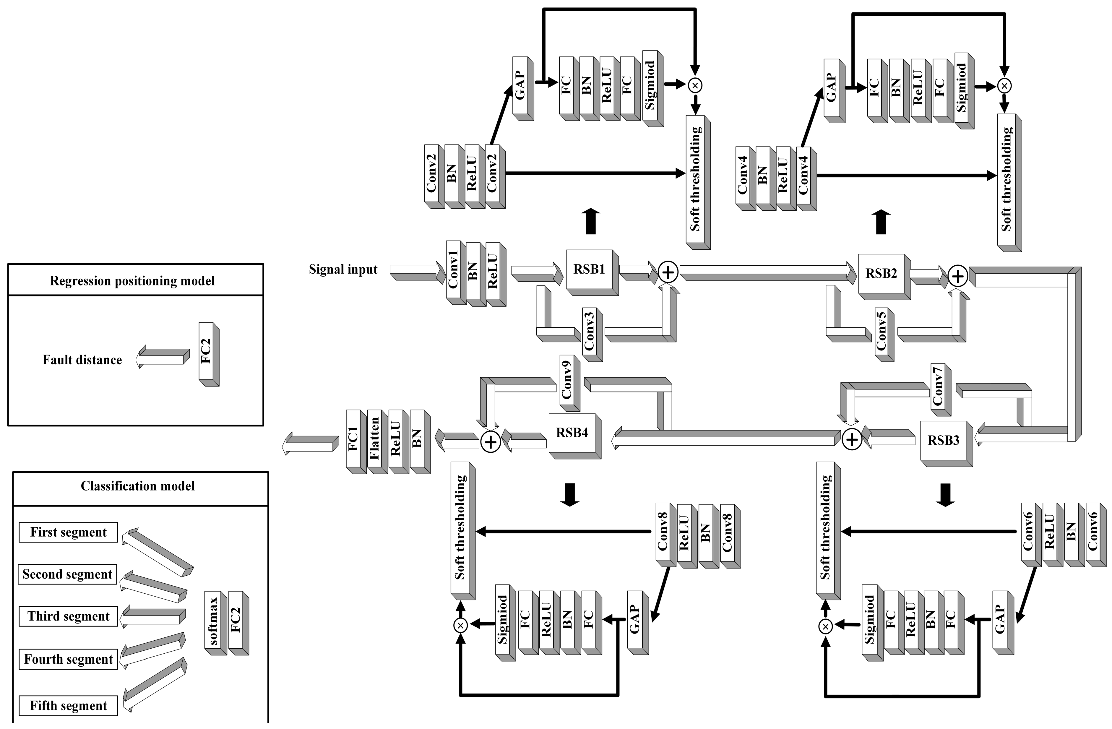
Innovatively proposing a high-resistance grounding fault location strategy for HVDC transmission systems based on the DRSN. This article is the first to introduce the DRSN into high-resistance grounding fault location for HVDC transmission systems, constructing a one-dimensional Deep Residual Shrinkage Network (1D-DRSN) model for fault location in HVDC transmission systems. This model accurately locates high-resistance grounding faults in HVDC transmission systems by deeply mining and learning the deep-level features in the fault signals after preprocessing and VMD.
Simulation verification is adopted to align more with engineering practice. This article employs the PSCAD/EMTDC software to build a ±800 kV bipolar HVDC transmission system model for fault simulation, incorporating actual engineering line parameters. Considering the difficulties in detecting and locating high-resistance grounding faults in HVDC transmission systems and actual equipment sampling precision limitations, the signal sampling frequency is set to the highest frequency of 10 kHz commonly found in DC projects. Simulation verification of high-resistance grounding faults with a wide range of grounding transition resistance values (800–5800 Ω) is conducted. Comparative experiments with traditional double-ended traveling wave methods based on modal maxima and fault location methods based on Convolutional Neural Network (CNN) demonstrate the proposed method’s superior positioning accuracy under high-resistance grounding faults and its robustness against noise interference in the data.
The rest of this article is organized as follows.
Section 2 presents the overall process of the fault location method based on the DRSN.
Section 3 describes the construction of input data for the DRSN model, including double-ended traveling wave sampling, phase-mode transformation, and Variational Mode Decomposition.
Section 4 introduces the Deep Residual Shrinkage Network model, including the specific design of the 1D-DRSN. In
Section 5, a ±800 kV HVDC transmission system is built in the electromagnetic transient simulation software PSCAD/EMTDC, and the effectiveness of the proposed method is evaluated under different fault distances and noisy conditions. Finally,
Section 6 draws the conclusion, summarizing the main contributions and limitations of the proposed method, and outlining directions for future research.
5. Simulation System and Simulation Verification Results
5.1. Modeling of HVDC Transmission Systems
PSCAD/EMTDC is a widely used electromagnetic transient simulation software in the field of power systems. It is a powerful tool for analyzing and studying issues such as DC transmission systems and the interaction between Alternating Current (AC) and DC systems. The version of PSCAD/EMTDC adopted in this article is 4.6.2. In this article, the PSCAD/EMTDC software is used to build a ±800 kV bipolar HVDC transmission system, as shown in
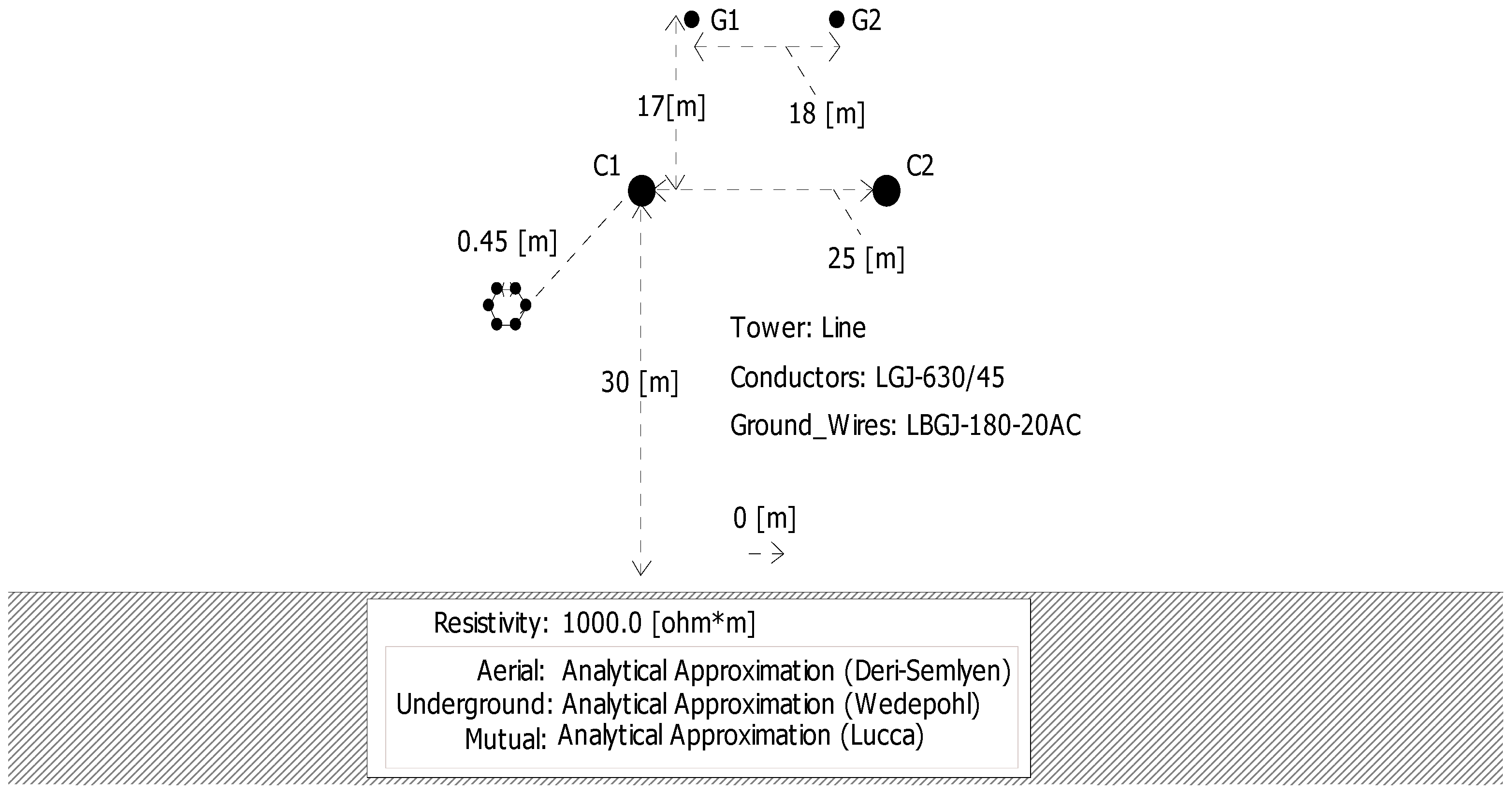
Figure 6. The HVDC transmission system adopts a 12-pulse converter valve, and both the rated capacity of the rectifier station and the inverter station are set to 2000 MW. The control system of the rectifier station utilizes constant current control and minimum triggering angle control, while the inverter station employs constant extinguishing angle control and constant current control. The inductance of the flat wave reactor is set to 0.4 H. The total length of the transmission line is 1000 km, and the geometric distribution of the line is shown in
Figure 7. The detailed parameters of the line are presented in
Table 2.
In the simulation analysis of this article, the fault time is set at t = 0.6 s, and waveforms are sampled for approximately 20 ms after the fault occurs. Considering the sampling limitations of actual engineering equipment, the sampling frequency is set to 10 kHz, resulting in 202 sampling points. The oscilloscopes at the inverter side and rectifier side can capture the superimposed signals of multiple fault traveling waves arriving at both ends, resulting from the mutations triggered by the fault.
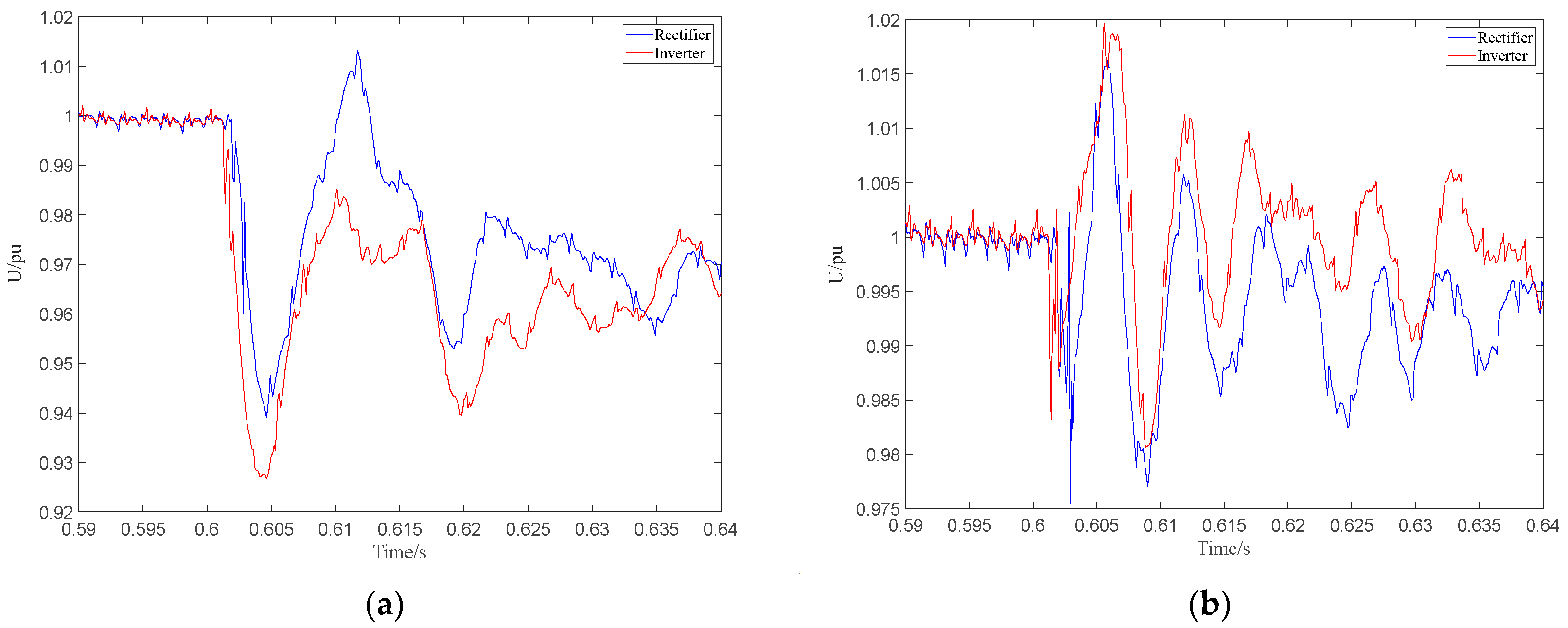
The line section of a HVDC transmission system mainly consists of positive and negative lines, and possible fault conditions include positive line faults, negative line faults, and bipolar line faults. Since the probability of simultaneous high-resistance grounding faults on both bipolar lines is extremely low, this article only considers positive line faults and negative line faults. Using the established ±800 kV HVDC transmission system, high-resistance grounding fault experiments are conducted on the positive and negative lines. The fault point is set at a distance of 400 km from the inverter terminal, with a grounding transition resistance of 2000 Ω, and the fault initiation time is set to 0.6 s.
Figure 8 shows the instantaneous voltage waveforms on both sides of the line for various fault conditions. The voltage waveform for a positive line fault is shown in
Figure 8a, and the voltage waveform for a negative line fault is shown in
Figure 8b. As shown in
Figure 8, when a high-resistance grounding fault occurs in an HVDC transmission system, the voltages measured at both ends exhibit vibrations. Still, the amplitude of these vibrations is relatively small. Therefore, in practical engineering, it is often difficult to accurately detect the presence of high-resistance grounding faults.
5.2. Variational Mode Decomposition Processing
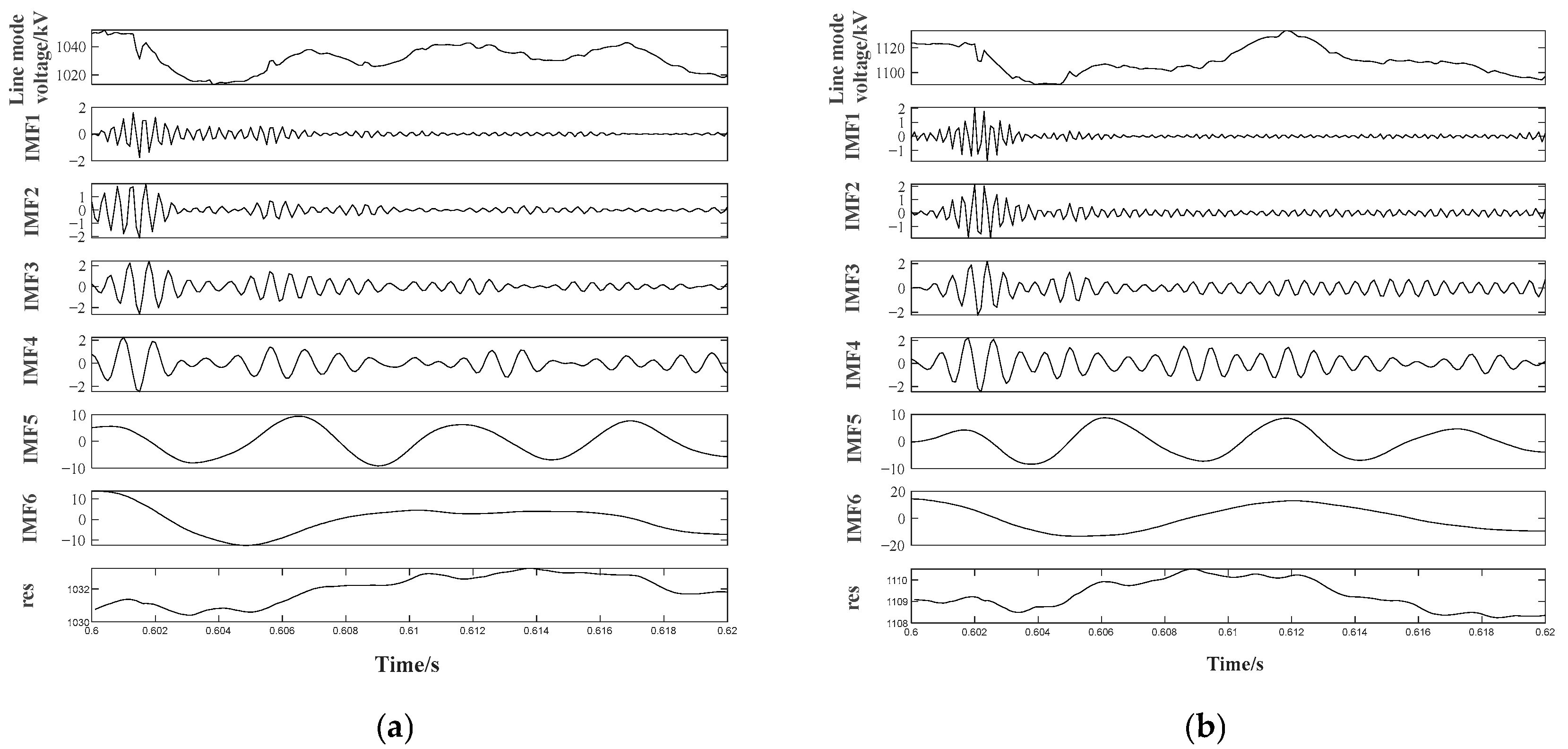
Taking the positive high-resistance grounding fault with a fault point at 400 km from the inverter and a grounding resistance of 2000 Ω as an example, the waveform 0.02 s after the fault occurrence at 0.6 s is extracted as the fault segment and decoupled into a line mode component through phase-mode transformation. The decomposition results of the original fault signal line mode component data at the rectifier and inverter terminals using VMD are shown in
Figure 9. It can be seen from the figure that VMD can effectively eliminate the volatility of the original fault signal and effectively extract the high-frequency characteristics of the fault voltage signal line mode component. After VMD, the IMF1 components at the rectifier and inverter terminals are normalized and concatenated into one-dimensional data to construct the training and testing data for the subsequent input to the DRSN.
5.3. Generation Forms of Training and Testing Data
The training data are generated in the following manner: In the established ±800 kV bipolar HVDC transmission system model with a total length of 1000 km, starting from a point 1 km away from the inverter-side recorder on both the positive and negative poles, high resistance grounding faults with transition resistances ranging from 1000 Ω to 2900 Ω in increments of 100 Ω are set every 1 km. These transition resistances are modeled as purely resistive components (only R components) that remain constant over time. This assumption is made to simplify the simulation and focus on the performance of the fault location methods under varying fault resistance conditions. A total of 39,960 fault samples were generated, including 19,980 positive pole fault samples and 19,980 negative pole fault samples, with each fault point corresponding to 40 fault samples. These training data are then utilized to train a 1D-DRSN and a 1D-CNN. For comparison, the 1D-CNN adopts the regression CNN model structure from reference [
7].
The testing data are generated as follows: Starting from a point 50 km away from the inverter-side recorder on both the positive and negative poles, high-resistance grounding faults with transition resistances ranging from 800 Ω to 5800 Ω in increments of 1000 Ω are set every 100 km. This configuration generates testing data samples for positive and negative pole faults.
After experimental debugging, the parameters for the 1D-DRSN are set as follows: batch_size is 10, validation_split is 0.2, the number of iterations is 500, and the optimizer is Adam. The deep learning program is developed in the PyCharm 2020.1 integrated development environment using the TensorFlow 2.6.0 framework. The hardware specifications include a Windows 11 (64-bit) operating system, 16 GB of RAM, a Core i5-12500H CPU (Intel, Santa Clara, CA, USA), an RTX 3050 GPU (Nvidia, Santa Clara, CA, USA), and a clock speed of 3.39 GHz.
5.4. Comparative Analysis of Simulation Verification Results
Fault location is performed on the testing data samples using three methods: the traditional double-ended modal maximum traveling wave method [
25], the 1D-CNN-based fault location method, and the 1D-DRSN-based fault location method. To quantify the detection precision, the Relative Mean Absolute Error (RMAE) is calculated for each method. The RMAE is defined as:
where
is the predicted fault distance for the i-th sample,
is the actual fault distance,
N is the total number of test samples, and
L is total length of transmission line.
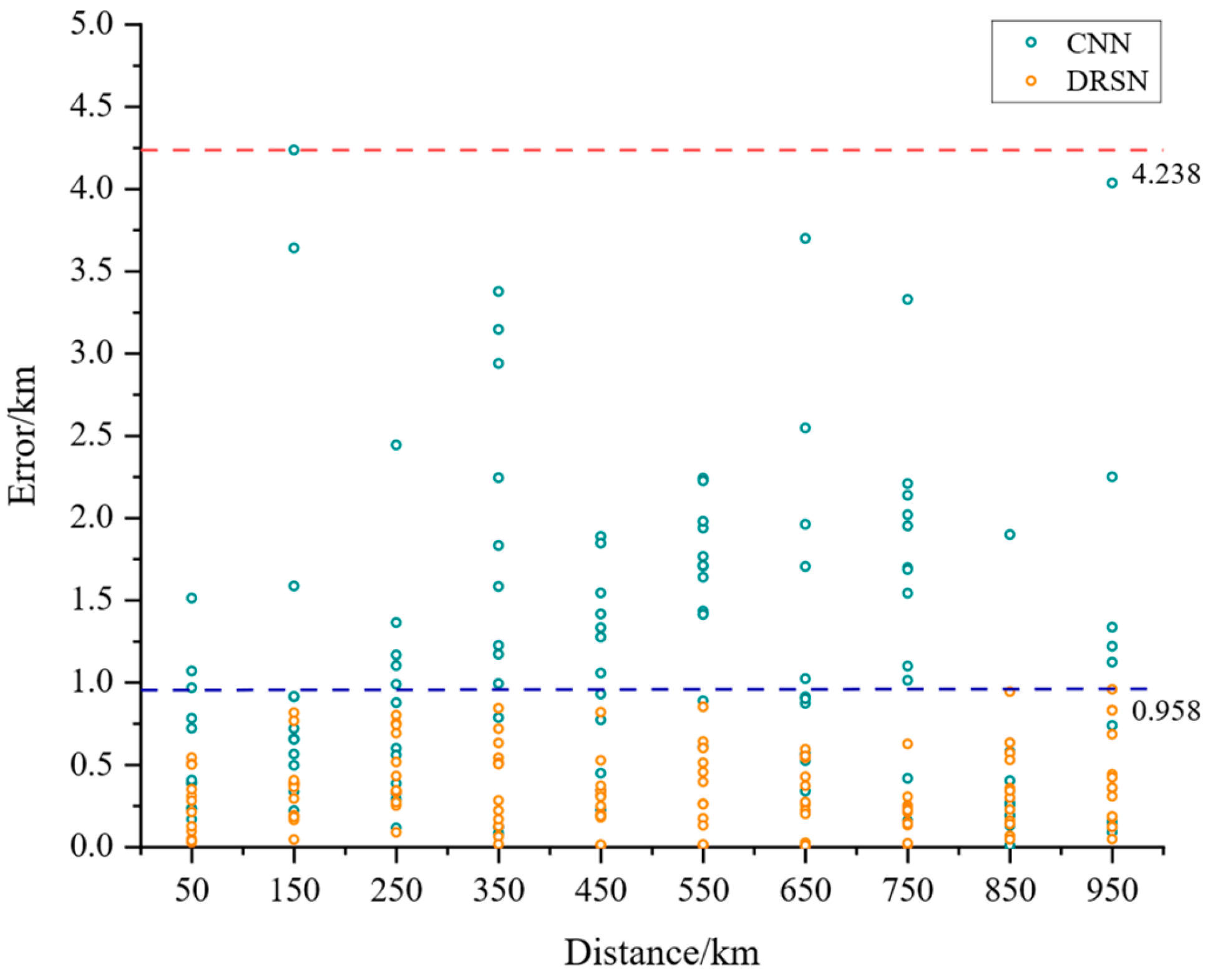
The ‘Distance’ value is obtained for each fault point by averaging the location results of 12 different fault pole types and different transition resistances in the testing data. The ‘Error’ value is then calculated as the average of the absolute values of the localization error results from these 12 different fault pole types and different transition resistances. The results are presented in
Table 3. The error distribution of the measurement results for each fault point using the 1D-CNN-based fault location method and the 1D-DRSN-based fault location method is shown in
Figure 10.
As can be seen from
Table 3 and
Figure 10, and the RMAE values, in the case of a single-pole high-resistance grounding fault with a transition resistance ranging from 800 Ω to 5800 Ω, the average absolute error of the traditional double-ended modal maximum traveling wave method for fault location is 17.312 km. This indicates that the conventional double-ended traveling wave method has a relatively large location error in high-resistance fault scenarios. The maximum error of the 1D-CNN method for fault location is 4.238 km, with an average error of 1.210 km and an RMAE of 0.1210%. The maximum error of the 1D-DRSN method is 0.958 km, with an average error of 0.343 km and an RMAE of 0.0343%. The localization error based on the 1D-DRSN method is primarily distributed between 0 km and 1 km, whereas a significant portion of errors based on the 1D-CNN method is distributed between 1 km and 4 km. Therefore, under the engineering sampling accuracy with a sampling frequency of 10 kHz, the 1D-DRSN-based fault location method exhibits higher accuracy than the 1D-CNN-based method for high-resistance grounding fault location. Furthermore, through testing, it has been verified that the overall output speed of the localization process based on the 1D-DRSN method can reach the order of seconds, satisfying the requirements of practical engineering applications.
5.5. Anti-Interference Analysis
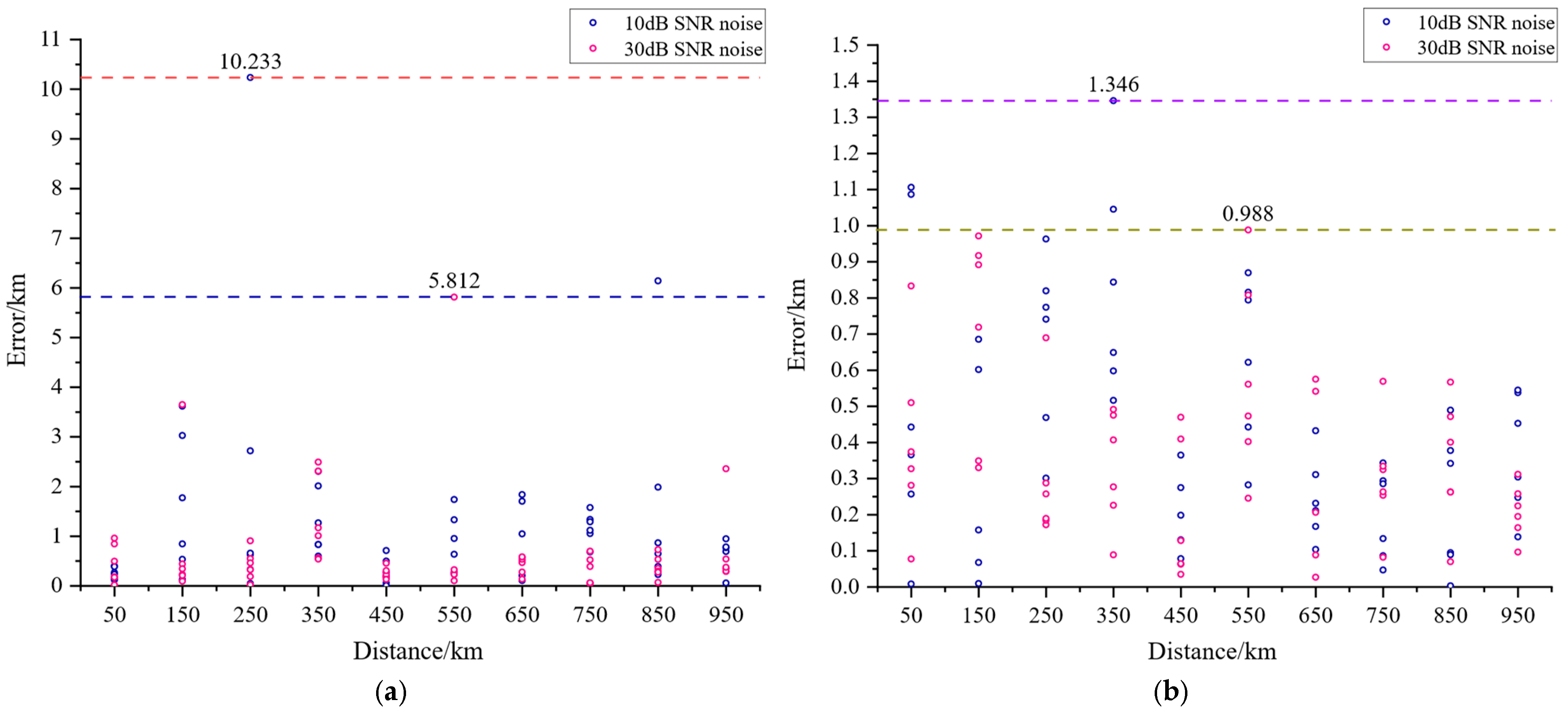
In practical HVDC transmission engineering, signals recorded by fault recorders are often contaminated by noise originating from inherent equipment noise and electromagnetic interference within the converter station valve hall environment. To evaluate the robustness of the proposed method under noisy conditions, Gaussian noise with Signal-to-Noise Ratios (SNRs) of 30 dB and 10 dB were deliberately introduced into the original fault signals. This noise level falls within a reasonable range for assessing the anti-interference capabilities of fault location methods. Subsequently, fault location was performed using both the fault location method based on 1D-CNN and the fault location method based on 1D-DRSN. For each fault location scenario, six distinct transition resistance points were selected from the testing data to generate noisy testing data for the purpose of fault location analysis. The positioning outcomes of the 1D-CNN-based method under Gaussian noise conditions with SNR of 30 dB and 10 dB are illustrated in
Figure 11a, whereas the positioning outcomes of the 1D-DRSN-based method are presented in
Figure 11b.
As can be seen from the location results shown under different Gaussian noise conditions
Figure 11a,b, in the scenario where Gaussian noise with an SNR of 30 dB is added to the signal, the maximum error of the fault location method based on the 1D-CNN reaches 5.812 km. In contrast, the maximum error of the high-resistance fault location method based on the 1D-DRSN is 0.988 km. In the scenario where Gaussian noise with an SNR of 10 dB is added to the signal, the maximum error of the fault location method based on the 1D-CNN reaches 10.233 km. In contrast, the maximum error of the high-resistance fault location method based on the 1D-DRSN is 1.346 km. Under different noise scenarios, the results of the method proposed in this article are relatively less affected by noise, with the maximum error not exceeding 1.5 km, which meets the engineering accuracy requirements.
The reason why the 1D-DRSN-based method strongly suppressed Gaussian noise compared to the conventional 1D-CNN-based method lies in its robust architecture. The 1D-DRSN employs a deep residual network, which allows the model to learn and adapt to the underlying patterns in the data while effectively filtering out noise. The residual learning mechanism enables the network to learn from the residuals between the input and the output, facilitating the capture of noise-resistant features. Additionally, the incorporation of attention mechanisms and soft thresholding operations in the 1D-DRSN further enhances its ability to distinguish between useful signals and noise, thus significantly improving its noise suppression capabilities. In contrast, conventional 1D-CNN methods may not be as effective in dealing with noise, as they often rely on simpler architectures that may not fully capture the complex patterns and noise-resistant features inherent in the data.
From the noise test results, it can be concluded that the high-resistance fault location method based on the 1D-DRSN has better network anti-interference performance than the fault location method based on the 1D-CNN.
6. Conclusions
This article proposes a fault location method for HVDC transmission lines based on DRSN, aiming to achieve accurate localization of high-resistance grounding faults on transmission lines. The input data are constructed after preprocessing using VMD for feature engineering by collecting double-ended fault voltage waveforms and performing phase-mode transformation. The 1D-DRSN is employed for classification and segmentation, followed by precise regression output for locating results in each segment. The proposed method is tested using a simulation model of an HVDC transmission line built with PSCAD/EMTDC. The test results indicate that in scenarios involving high-resistance grounding faults and considering the sampling accuracy of engineering equipment, the traditional double-ended modal maximum traveling wave method exhibits relatively large localization errors. However, the fault location method based on the DRSN demonstrates high localization accuracy and holds certain advantages over the method based on the 1D-CNN. Considering the presence of noise in signals in practical engineering applications, the fault location method based on the DRSN exhibits a maximum error of less than 1.5 km, showing a more substantial robust network anti-interference capability compared to the 1D-CNN-based method while also meeting engineering accuracy requirements.
Although the DRSN-based fault location method for HVDC transmission lines is effective, it exhibits several limitations that necessitate further exploration and potential refinements. One major limitation is the substantial amount of training data required, as the model’s performance is highly dependent on the availability and quality of these data. Gathering a comprehensive dataset that covers various fault scenarios and transition resistances can be both time-consuming and costly. Another issue is that, while the method shows high accuracy for high-resistance grounding faults within a certain range, its performance may degrade when faced with a wider range of transition resistances, indicating the need for further optimization of the model architecture and training strategies. Additionally, the trained model may not function optimally when applied to a new HVDC transmission line without retraining on specific data from that line, due to differences in electrical characteristics and parameters. To address these challenges, future research should concentrate on reducing data dependency, enhancing model generalization, and developing adaptable or transferable DRSN models.
Meanwhile, the validity of the proposed high-resistance grounding fault location method is primarily demonstrated through simulation verifications utilizing PSCAD/EMTDC software in this article. When introducing new methods into power systems, formal verification techniques, such as statistical model checking, can also be applied to provide a more stringent and comprehensive validation process. This aids in ensuring the correctness and reliability of the new methods. Consequently, in future research, a more holistic justification for the adoption of new methods can be achieved by integrating simulations, experiments, and formal verification, thereby further promoting their application in power systems.


