Abstract
Oriented object detection has become a hot topic in SAR image interpretation. Due to the unique imaging mechanism, SAR objects are represented as clusters of scattering points surrounded by coherent speckle noise, leading to blurred outlines and increased false alarms in complex scenes. To address these challenges, we propose a novel noise-to-convex detection paradigm with a hierarchical framework based on the scattering-keypoint-guided diffusion detection transformer (SKG-DDT), which consists of three levels. At the bottom level, the strong-scattering-region generation (SSRG) module constructs the spatial distribution of strong scattering regions via a diffusion model, enabling the direct identification of approximate object regions. At the middle level, the scattering-keypoint feature fusion (SKFF) module dynamically locates scattering keypoints across multiple scales, capturing their spatial and structural relationships with the attention mechanism. Finally, the convex contour prediction (CCP) module at the top level refines the object outline by predicting fine-grained convex contours. Furthermore, we unify the three-level framework into an end-to-end pipeline via a detection transformer. The proposed method was comprehensively evaluated on three public SAR datasets, including HRSID, RSDD-SAR, and SAR-Aircraft-v1.0. The experimental results demonstrate that the proposed method attains an of 86.5%, 92.7%, and 89.2% on these three datasets, respectively, which is an increase of 0.7%, 0.6%, and 1.0% compared to the existing state-of-the-art method. These results indicate that our approach outperforms existing algorithms across multiple object categories and diverse scenes.
1. Introduction
Synthetic Aperture Radar (SAR) is capable of operating under all-day and all-weather conditions and has found widespread applications across numerous domains [1,2,3]. As spaceborne SAR advances rapidly, SAR object detection [4,5] has drawn a lot of attention. As a recently emerged challenging task, oriented object detection (OOD) is particularly well suited for SAR objects characterized by arbitrary orientation, a wide range of aspect ratios, and blurred outlines. Over the past decade, researchers have delved into this field, leading to remarkable advancements.
Traditional SAR object detection methods represented by the constant false alarm rate (CFAR) [6] typically involve the statistical modeling of specific scenes in SAR images. Nevertheless, the significant challenges in accurately modeling the statistical distribution of complex scenes lead to limited feature representation and reduced robustness. With the development of deep learning, convolutional neural networks (CNNs) have been widely utilized in SAR object detection [7,8]. Compared to traditional methods, CNN-based approaches offer powerful, robust feature representation and automatic feature extraction capabilities [9,10]. However, most existing CNN-based detectors [11,12,13] are typically designed for optical images. The significant domain differences between optical and SAR images introduce new challenges, limiting the advancement of deep learning in SAR object detection.
First, objects in optical images typically have clear and well-defined boundaries. In contrast, SAR images represent objects as clusters of scattering points due to its unique imaging mechanism. These clusters are dominated by a few strong scatters that appear as bright spots, while the remaining areas appear dark due to weak or negligible backscatter. Additionally, the coherent speckle noise in the surrounding background often disrupts object boundaries, further complicating their delineation. As a result, object outlines in SAR images are often shown as blurred and irregular. Early methods [14,15], inspired by optical detectors, directly used a simplified horizontal bounding box (HBB) to represent the object outline. However, this representation only provides coarse boundary information and often includes non-target areas. To address this issue, recent research [16,17] utilizes the oriented-bounding-box (OBB) representation, which incorporates precise scale and orientation information to obtain more accurate object outlines, resulting in significant improvements.
Second, the distribution of scattering-point clusters in specific background areas, such as ports or terminals, often closely resembles that of objects. This resemblance makes it challenging to distinguish these areas from actual objects. As a result, these similarities frequently lead to false alarms, thereby reducing the detection accuracy [18]. A common approach to address this issue involves using post-processing algorithms [19], which evaluate the saliency of predictions relative to the background to filter out less prominent detections. However, this method lacks robustness and requires an additional post-processing step, preventing the implementation of an end-to-end detection pipeline. Recent research [9] proposes directly training neural networks to learn saliency information by integrating it into the detection framework. The effectiveness of this approach heavily depends on the quality of the additionally saliency maps used during training, which are challenging to produce with high fidelity. To overcome this limitation, recent methods [20,21,22] leverage attention mechanisms to capture contextual and global information, effectively suppressing false alarms and achieving promising results.
Despite the notable advancements achieved by the methods mentioned above, considerable challenges remain. First, the OBB representation remains inherently rectangular, which limits its ability to capture details of the blurred and irregular object outlines, as shown in Figure 1. Some studies [18,23] have attempted to improve OBB predictions by directly generating a scattering-point heatmap. However, these methods are computationally expensive and heavily depend on additional high-quality annotations to accurately guide the heatmap prediction. Moreover, they continue to use OBB as the final object-outline representation, which restricts their capability to describe complex object geometries. Recently, Guo et al. [24] introduced irregular quadrilaterals to more accurately represent object outlines. While this approach addresses the limitations of rectangular OBBs, it still lacks the granularity needed to fully capture blurred and irregular outlines. Second, existing context modeling approaches often apply attention mechanisms to SAR images in a stationary paradigm, without adequately considering the unique characteristics of SAR imagery. Specifically, these methods [20,25] directly use attention mechanisms to establish long-range relationships within rectangular regions of interests (RoIs). However, these RoIs often encompass non-target scattering points, which interfere with the accurate extraction of context and global information. Some studies [21,26,27] have developed specialized modules to capture the relationships between scattering points or regions. Nonetheless, these methods are typically object-specific, requiring additional supervision or auxiliary algorithms, which limits their generalizability and efficiency.
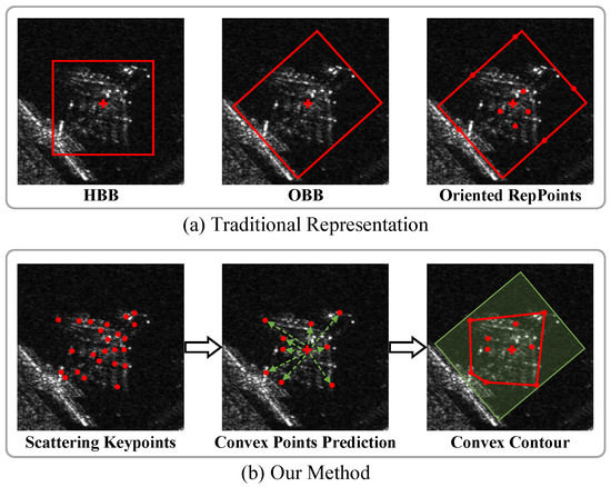
Figure 1.
(a) Traditional object-outline modeling representations are displayed from left to right: the horizontal bounding box; the oriented bounding box; and the adaptive RepPoints. The red rectangle represents the bounding boxes, the red crosses indicate the object centers, and the red dots denote RepPoints. (b) Compared to traditional representations, our method adaptively captures the object-scattering keypoints and integrates their features to predict a precise convex contour, which provides a fine-grained description for the object’s blurred outline. The red dots represent corresponding scattering keypoints or convex points, red lines form the convex contour, green dashed lines indicate offsets of points, and the green rectangle indicates the object’s area.
To tackle these problems, a novel noise-to-convex detection paradigm is proposed in this article. This paradigm adopts a hierarchical framework based on the scattering-keypoint-guided diffusion detection transformer (SKG-DDT), comprising three specialized modules that progressively obtain the object’s blurred outline. First, a strong-scattering-region generation (SSRG) module is introduced at the bottom level. This module utilizes a diffusion model to learn the spatial distribution of strong scattering regions, providing approximate object regions. Then, a scattering-keypoint feature fusion (SKFF) module is designed at the middle level. Leveraging the identified regions from the bottom level, this module dynamically detects object-scattering keypoints across multiple scales and constructs their spatial and structural relationships using the attention mechanism. By combining these keypoint features, the SKFF module effectively captures both object structure and contextual information. Additionally, it interacts with the SSRG module to further suppress background regions. Finally, a fine-grained convex contour representation and a convex contour prediction (CCP) module are introduced at the top level. This module adaptively predicts precise convex contours of objects using the coarse object regions from the bottom level and the combined scattering-keypoint features from the middle level. Furthermore, the detection transformer is employed to integrate and uniformly model the three modules across the hierarchical levels, enabling end-to-end oriented object detection for representative SAR objects (ship and plane) without any post-processing algorithms.
The main contributions of this article are summarized as follows:
- (1)
- This article introduces a novel noise-to-convex detection paradigm, which employs a hierarchical three-level framework that integrates SAR-specific mechanisms with deep learning methods, progressively obtaining a fine-grained convex contour description of the blurred object outline.
- (2)
- A strong-scattering-region generation (SSRG) module is developed at the bottom level. This module utilizes a diffusion model to learn and construct the spatial distribution of strong scattering regions, enabling the direct identification of approximate object regions.
- (3)
- A scattering-keypoint feature fusion (SKFF) module is introduced at the middle level. This module adaptively detects scattering keypoints and fuses their features, effectively enhancing the object feature and reducing false alarms in complex scenes.
- (4)
- A convex contour representation and convex contour prediction (CCP) module is proposed at the top level to obtain a precise and fine-grained convex contour for the object outline.
2. Related Work
2.1. Modeling Methods for SAR Object Outline
In SAR images, objects are represented as clusters of scattering points, dominated by a few strong scatters that appear as bright spots. These scattering clusters result in objects with irregular contours, while the coherent speckle noise in the surrounding background further disrupts object boundaries. Consequently, the outlines of SAR objects are often shown as blurred and irregular. Early methods, inspired by general detectors [11,12,13], approximated SAR object outlines using simplified horizontal bounding boxes (HBBs). For instance, Wang et al. [14] used the single-shot multibox detector (SSD) to predict HBB outlines. However, the HBB representation provides only coarse boundary information and often fails to tightly enclose objects. Therefore, recent research shifted to the oriented-bounding-box (OBB) representation, which incorporates precise scale and orientation information to obtain more accurate object outlines. DRBox-v2 [17] combined the SSD framework with a multi-layer prior box generation strategy to refine OBB predictions. FPDDet [28] employed a five-parameter polar coordinate system to avoid discontinuities when predicting angle information. FADet [29] utilized the spatial and channel attention mechanism to design an adaptive boundary enhancement module that implicitly improves OBB accuracy.
Despite these advancements, the OBB representation remains insufficient for capturing the intricate details of blurred and irregular object outlines. To overcome the limitations of OBB, Sun et al. [23] and Sun et al. [18] proposed directly generating scattering-point heatmaps to better capture object boundary details. SRT-Net [27] enhanced object contours by clustering predicted scattering points across the image, resulting in improved detection performance. However, these methods still rely on OBB for final outline representation and require additional annotations or auxiliary algorithms to guide the scattering-point prediction. More recently, Guo et al. [24] adopted irregular quadrilaterals to better describe object outlines. While this approach overcomes the rigidity of regular rectangle, it still lacks the granularity needed to capture blurred and irregular boundaries. In response to these challenges, we propose a fine-grained convex contour representation, which more effectively captures the object outline in SAR imagery.
2.2. Context Modeling Methods for SAR Object Detection
In SAR images, certain areas of the complex background often exhibit visual attributes similar to objects, making it challenge to distinguish them. Therefore, leveraging the context and global information becomes essential for effectively identifying objects. To address this challenge, Kang et al. [30] and Chen et al. [31] projected region proposals onto multiple layers with region of interest (RoI) pooling, extracting both RoI features and contextual information. With its ability to capture long-range relationships, the attention mechanism has become a widely used tool for extracting context in SAR images. For instance, DAPN [20] densely connected the convolutional block attention module (CBAM) concatenated feature maps of a pyramid network, capturing both global and contextual information. AFRAN [25] utilized an attention feature fusion module to refine and fuse low-level texture and high-level semantic features. FADet [29] introduced a feature alignment module (FAM) into the feature pyramid network (FPN), which aligns fine-grained semantic information through semantic flow alignment to enhance discriminative object features. FPDDet [28] designed a feature enhancement (FE) module incorporating position attention and channel attention, enhancing object features while suppressing background interference.
However, these methods apply attention mechanisms to SAR imagery without considering the characteristics of SAR imagery. Recognizing the importance of scattering points for context extraction, Fu et al. [32] utilized a predefined Gaussian mixture model to extract scattering-structure features. Fu et al. [26] proposed a context-aware feature selection module to dynamically learn local and contextual features based on strong scattering points. SRT-Net [27] introduced a scattering-region topological structure pyramid to dynamically capture global context and enhance ship saliency. However, these methods are tailored to a specific object category and depend heavily on additional supervision or auxiliary algorithms. In contrast, we propose an adaptive learning approach applicable to multiple object categories and diverse scenarios.
2.3. Diffusion Models
Recently, diffusion models have demonstrated remarkable capabilities in understanding image content for generative tasks [33,34,35] and have been increasingly applied to perception tasks [36,37], such as object detection and segmentation. DiffusionDet [37], the first to apply the diffusion model to object detection, introduced a novel noise-to-box detection paradigm. In this paradigm, object detection is framed as a diffusion denoising process, transforming noisy boxes into precise object boxes. This approach highlights the effectiveness of the diffusion model in constructing the spatial distribution of object regions in optical images. Additionally, it eliminates the need for densely sampled region proposals, reducing false alarms caused by excessive sampled background candidates, which is a significant advantage for SAR imagery. In SAR images, most existing applications of the diffusion model have focused on tasks such as despeckling [38] or data augmentation [39]. To date, there have been no attempts to explore the potential of the diffusion model specifically for SAR object detection. Given the unique challenges of SAR imagery, such as coherent speckle noise and blurred object boundaries, a thorough investigation into the application of the diffusion model for SAR object detection is both timely and necessary.
3. Methods
The hierarchical three-level framework of the proposed SKG-DDT is illustrated in Figure 2. This framework progressively generates a fine-grained convex contour description of the blurred object outline in a coarse-to-fine manner. At the bottom level, the SSRG module learns the spatial distribution of scattering regions through a diffusion denoising process, directly approximating object regions. Building on these approximated regions, the SKFF module dynamically detects scattering keypoints across multiple scales at the middle level. An attention mechanism is then employed to establish spatial and structural relationships among these keypoints, combining their corresponding features into the final scattering-keypoint feature. Finally, at the top level, the CCP module adaptively predicts the precise object convex contour by leveraging both the regions from the bottom level and the scattering-keypoint feature from the middle level.
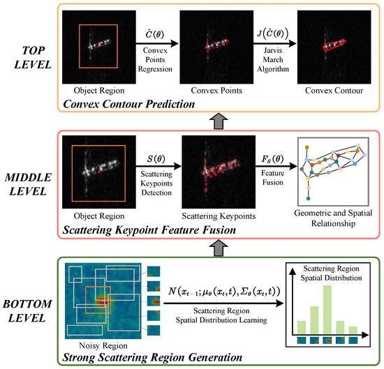
Figure 2.
The hierarchical framework of the proposed method. Bottom level: approximate object regions are generated by learning the spatial distribution of strong scattering regions. Middle level: scattering keypoints are located based on the bottom-level region, then their features are combined for geometric insight. Top level: the convex contour is refined by leveraging both the bottom-level region and the middle-level keypoint features. The orange rectangle denotes the object region, red dots are scattering keypoints or convex points, and red lines form the convex contour.
The overall network architecture of SKG-DDT is depicted in Figure 3. It utilizes a standard backbone and a channel mapper [13] to extract multi-scale features, which are then processed through a detection transformer head. This head comprises a 6-layer deformable DETR encoder [40], along with the SSRG, SKFF and CCP modules. Each level of the hierarchical framework is detailed in the subsequent subsections. Additionally, the final subsection introduces the dynamically weighted CIOU (DW-CIOU) loss, specifically designed to enhance model supervision during training, and discusses the components of the total loss.
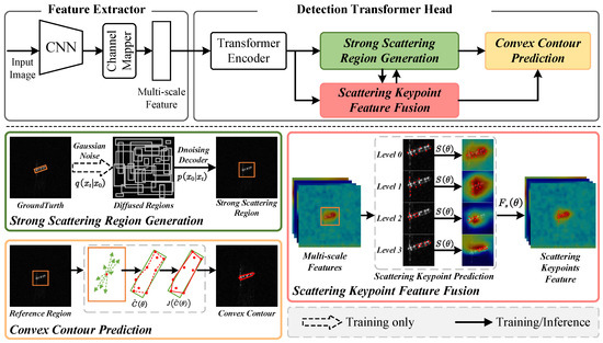
Figure 3.
The architecture of the proposed method consists of a feature extractor and a detection transformer head. The feature extractor uses a backbone and a channel mapper to extract multi-scale features. The detection transformer head includes a 6-layer transformer encoder, along with the SSRG, SKFF, and CCP module. The orange rectangle denotes the object region, red dots are scattering keypoints or convex points, green dashed lines indicate offsets of points, and red lines form the convex contour.
3.1. Strong-Scattering-Region Generation Module
Objects in high-resolution SAR images typically consist of sparsely distributed clusters of scattering points, which visually manifest as strong scattering regions. Inspired by DiffusionDet [37], we propose the strong-scattering-region generation (SSRG) module at the bottom level. This module leverages a diffusion model to learn the spatial distribution of strong scattering regions, enabling the direct extraction of approximate object regions. This approach allows subsequent processes to concentrate on object regions while effectively filtering out irrelevant background interference. A significant advantage of the SSRG module is that it eliminates the need for additional high-quality ground truths, relying solely on existing annotations from the detection task for training. Specifically, the largest enclosing horizontal rectangles are calculated from the objects’ OBB annotations and expanded by a factor of 1.2 to serve as the ground truth for this module.
3.1.1. Strong-Scattering-Region Spatial Distribution Learning
As a kind of likelihood-based model inspired by non-equilibrium thermodynamics [41], the diffusion model [33] defines a Markovian chain of diffusion processes by gradually adding noise to the sample data. During training, we firstly construct the diffusion process from ground-truth (GT) strong scattering regions to noisy regions, which transforms data sample to the noisy samples by gradually adding Gaussian noise at each timestep to . The diffusion process is defined as follows:
where and represents the noise variance schedule. Data sample is a set of GT strong scattering regions and denotes noisy regions. We represent the strong scattering region by HBB as normalized coordinates , where are the center coordinates and are the width and height of the region. In addition, we directly utilize the minimum horizontal rectangle of OBB annotations as the GT strong scattering regions. The setting of hyperparameters in the diffusion process is consistent with DiffusionDet [37].
Then, we train a neural network to implement the denoising process that reverses the diffusion process. Specifically, the data sample is reconstructed from noise sample via the neural network and a progressive updating schedule, i.e., . In this article, we directly train a neural network to predict from , conditioned on the corresponding image feature . This approach enables us to directly generate potential object regions from noisy regions. To implement this, we utilize a transformer-based DETR decoder as the neural network for the denoising process, referred to as the denoising decoder. A detailed explanation of the denoising decoder is provided in Section 3.1.2.
The inference stage differs slightly from training, as it omits the diffusion process. Instead, it directly employs the denoising process to generate approximate object regions from noisy inputs.
3.1.2. Denoising Decoder
The denoising process of the SSRG module is implemented through the denoising decoder, which comprises six denoising-decoder layers. Each layer retains the multi-head self-attention mechanism from the DETR decoder, enabling it to capture long-range relationships between object features effectively. Given the unique characteristics of SAR images, we recognize the importance of object-scattering keypoints in guiding the extraction of meaningful object features. Therefore, the input to each denoising-decoder layer is also passed through the SKFF module to obtain the scattering-keypoint feature. Within the denoising decoder layer, cross-attention is utilized to extract discriminative object information from the scattering-keypoint feature, enhancing its capacity to identify target regions. To ensure consistent feature integration, each of the six denoising decoder layers is paired with a corresponding SKFF module.
Beyond processing noisy regions and the scattering-keypoint feature, the denoising decoder also incorporates conditional information derived from the noise timestep t. To explore the influence of this conditional information, we propose three variants of the denoising-decoder layer, each handling the conditional information differently. These designs, though involving small modifications, significantly impact the overall performance of the SSRG module. An illustration of all the designs is shown in Figure 4.
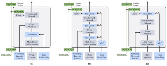
Figure 4.
Various designs of the denoising-decoder layer integrating the time-embedding condition: (a) Concatenation; (b) All layer adaptive layer normalization; (c) Single layer adaptive layer normalization. The blue boxes represent newly added structures or inputs, the green boxes indicate the noisy region, and the green lines indicates the information flow of noisy regions. For simplicity, the standard layer normalization after each multi-head self-attention, cross-attention, and feedforward network is omitted.
- (a)
- The embedding of the noise timestep t is concatenated with the input object queries and fed into the denoising decoder as new queries. This allows the module to implicitly learn the relationships between object features under varying noise conditions. Specifically, in the first layer, the time embedding is directly concatenated with the input object queries. In subsequent layers, the time embedding is concatenated with the processed object queries from the previous layer.
- (b)
- Inspired by the widespread usage of adaptive normalization layers [42] in GANs and diffusion models, we explore replacing all standard normalization layers in the denoising decoder with adaptive layer normalization (adaLN). Unlike standard normalization, adaLN conditions on the noise timestep t by regressing the scale and shift parameters and from its embedding. This approach applies the same conditioning function across all object queries, embedding the noise timestep information directly into the process of updating object features.
- (c)
- We replace only the standard normalization at the end of each denoising-decoder layer with adaLN, leaving other normalization operations unchanged. This introduces the noise timestep t solely at the layer outputs, reducing the number of parameters and computational complexity compared to replacing all standard normalization layers. We adopt this lightweight conditioning mechanism in our final design, as it achieves optimal performance according to our ablation studies.
Since the denoising decoder requires a fixed number of object queries, we concatenate random regions to the GTs prior to the diffusion process. This ensures that the number of diffused regions matches the number of object queries processed by the denoising decoder.
3.2. Scattering-Keypoint Feature Fusion Module
Scattering keypoints of SAR objects carry unique structural features and context information, which are crucial for accurately predicting convex contours and differentiating objects from background clutter. Building on insights from previous studies [21,27,43], we propose the scattering-keypoint feature fusion (SKFF) module. This module dynamically detects scattering-keypoint positions across multiple scales and then uses an attention mechanism to learn the structural and spatial relationships among these keypoints. By fusing the corresponding keypoint features, the module produces the final scattering-keypoint feature that integrates both the object’s structural attributes and its surrounding context. The scattering keypoints detected in the SKFF module are illustrated in Figure 5c. And the detailed architecture of the SKFF module is displayed in Figure 6.
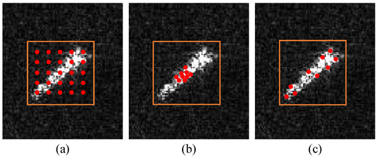
Figure 5.
A visualization of the predicted keypoints for different methods. For simplicity, we only visualized the scattering keypoints predicted at a certain scale in the SKFF module. (a) Attention; (b) deformable attention; (c) SKFF. The orange rectangle represents the object region, and red dots are keypoints.
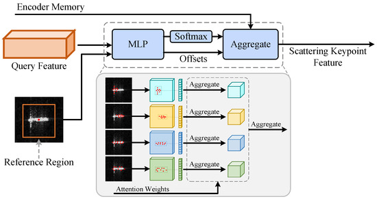
Figure 6.
The structure of the proposed SKFF module. It takes as input the query feature and the object region (reference region) from the SSRG module. Then, it dynamically localizes scattering keypoints at multiple scales and generates their corresponding attention matrix through the MLP. Based on the attention matrix, the features from these keypoints are effectively fused. The orange rectangle represents the object region, red dots are the detected scattering keypoints, the cuboids with four colors within the gray box represent feature maps at four scales.
3.2.1. Scattering-Keypoint Detection
We firstly define the scattering keypoints detected within each object region as
where k indexes the scattering keypoint and is the normalized coordinate of it. K represents the total number of scattering keypoints, which is set to 9 in this article.
Unlike methods that rely solely on single-scale predictions, multi-scale prediction offers significant advantages. At different scales, features capture complementary information, leading to the distribution of scattering keypoints across distinct regions of the object. At coarser scales, scattering keypoints are generally found around the object’s perimeter, capturing broader contextual information. In contrast, at finer scales, the predicted scattering keypoints emphasize detailed structures, such as the wings of an airplane or the bow and stern of a ship. This multi-scale approach thus yields a more comprehensive representation of the object’s structural and contextual attributes.
For each feature scale, we apply a two-layer MLP with SiLU activation to predict the corresponding scattering keypoints. Specifically, for each object region obtained in the SSRG module, let be the center coordinates of the region, and be its width and height. For the k-th scattering keypoint at the l-th scale, the network outputs normalized offsets from the region center. These offsets are then scaled by to obtain the actual displacements in the original coordinate space. Formally, the predicted scattering-keypoints set can be expressed as
In Equation (3), denotes the complete set of keypoints for each object, and represents the parameters of the MLP. In this notation, K is the number of keypoints at each scale, and L is the total number of scales. The terms and are the predicted normalized offsets for the k-th keypoint at the l-th scale, and correspond to the center coordinates, width, and height of the object region. All keypoint coordinates in are normalized to the range .
We use four distinct 2-layer MLPs, each with non-shared parameters, to process features at four different scales independently. These MLPs learn to locate scattering keypoints through direct optimization, without requiring any additional supervision. Each MLP’s input channel matches the dimensionality of the query feature, while its hidden dimension is set to four times the input channel. The output channel is configured as . The first channels encode the offsets , representing positional adjustments of the scattering keypoints. The remaining channels are then passed through a softmax operator to produce the attention matrix, which dynamically weights the importance of keypoints across scales. As shown in Figure 5, this method demonstrates state-of-the-art performance relative to other approaches.
3.2.2. Scattering-Keypoint Feature Fusion
After obtaining scattering keypoints across various scales, we employ an attention mechanism to model the structural and spatial relationships among these keypoints. Firstly, features at the scattering-keypoint locations are extracted from the corresponding multi-scale feature maps. Then, the attention matrix , derived from the last channels of the MLP output, is applied to perform a weighted fusion of these keypoint features. Finally, a linear layer with matching input and output dimensions aggregates the fused features into the final scattering-keypoint feature. The entire process can be mathematically formulated as
In Equation (4), is the integrated scattering-keypoint feature, and denotes the parameters of the MLP. Here, l indexes the feature scale, and k indexes the scattering keypoint. The term represents the l-th scale feature map, while rescales the normalized coordinates of the scattering keypoints to the spatial resolution of the l-th feature map. The matrix is a learnable weight that transforms the extracted features into a consistent representation space, and indicates the attention weight for the k-th keypoint at the l-th scale. By combining object structural and contextual information in this way, effectively enhances discriminative features, thereby suppressing false alarms and improving both object region identification and convex contour prediction.
3.3. Convex Contour Prediction Module
3.3.1. Convex Contour Representation
In SAR images, object outlines are usually blurred and irregular. Te better address this issue, and inspired by CFA [44], we introduce a fine-grained convex contour representation that provides a more accurate delineation of the object boundary. Unlike the OBB representation, which approximates an object’s outline with a single rectangle, our approach uses polygons composed of multiple points for a finer depiction of shape variation. Specifically, for each object region generated in the SSRG module, we define the predicted convex contour as a set of convex points, as
In Equation (5), C is the collection of convex points. The index n enumerates each convex point, and N is the total number of points in the convex point set. Initially, all convex points are placed at the center of the corresponding object region, providing a consistent initialization before further refinements. This design offers a more nuanced representation of the object boundary, which is particularly advantageous in SAR imagery where object contours are highly variable.
3.3.2. Convex Contour Regression
After obtaining the query feature from the SSRG module and the scattering-keypoint feature from the SKFF module, we concatenate them along the channel dimension and then process the concatenated feature with a linear layer to halve its channel number. A subsequent feedforward network (FFN), parameterized by , together with a sigmoid function, is employed to predict the normalized offsets for the n-th convex point relative to the center of the corresponding object region. The actual offsets for the n-th convex point are then obtained by scaling the normalized offsets with the width and height of the relevant object region. Let N be the total number of convex points to predict for each object region. We denote by the set of all predicted convex points, which can be computed by
and
In Equation (7), denotes the parameters of the FFN, and represent the width and height of the relevant object region, and is a hyperparameter that scales the predicted offsets, which is set to 1.5 in this work. The above process is computationally lightweight, and once these convex points are predicted, we apply the Jarvis March algorithm [45] to refine them. Specifically, let be the final convex contour for each object region, given by
where represents the Jarvis March algorithm. In practice, not all the initially predicted convex points in help form the actual convex contour, and updating some points may even degrade its shape, as illustrated in Figure 7. By applying , we select only the effective points to form , thereby improving the accuracy and robustness of the final convex contour prediction.
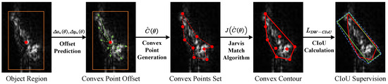
Figure 7.
An illustration of the convex contour prediction process. Starting from the object region (left), offset predictions generate a set of convex points . These points are refined into the final convex contour using the Jarvis March algorithm . The entire procedure is supervised by the dynamically weighted CIoU (DW-CIoU) loss to ensure robust contour alignment with ground truth. The orange rectangle represents the object region, red dots are convex points, green dashed lines indicate offsets of convex points, red lines form the convex contour, and the green rectangle is the ground truth box.
During training, the convex points are guided toward the ground-truth (GT) box using the Convex IoU Loss (CIoU Loss), which maximizes the Convex IoU (CIoU) between the predicted convex contour and the GT box, as illustrated in Figure 7. The definition of CIoU follows the formulation in CFA [44]. Unlike conventional methods that rigidly enforce alignment with the GT box, our approach employs the CIoU Loss to dynamically learn key boundary positions. This enables the model to produce a fine-grained and adaptive description of the object’s outline. Once the fine-grained convex contour is obtained, its minimum bounding rectangle can be readily extracted and used as the corresponding OBB or HBB representation. This flexibility highlights the superiority of the convex contour representation, which not only provides a detailed boundary description but can also be converted seamlessly into coarser representations for comparison with other detectors.
3.4. Dynamically Weighted CIoU Loss
As previously discussed, the convex contour is derived from the object region generated by the SSRG module. Consequently, the accuracy of the convex contour is strongly influenced by the quality of the object region. Samples with high-quality object regions contribute more effectively to the optimization of convex contour regression. Therefore, assigning equal weights to samples with varying object region quality during the optimization process is suboptimal, and may leads to inefficient learning.
To address this issue, we propose a dynamically weighted CIoU (DW-CIoU) loss. This loss adapts the contribution of each training sample in the CIoU loss according to the quality of its generated object region. In doing so, our method assigns higher weights to samples with more reliable object regions while still leveraging the learning potential of low-quality samples. Formally, we introduce a dynamic weight for the original CIoU loss:
In Equation (9), and are the generated object region from the SSRG module and the corresponding ground-truth (GT) region, respectively. The function represents the L1 distance, used to capture the magnitude of the discrepancy between and . The term measures the overlap ratio between the generated and ground-truth regions, serving as an indicator of the region’s quality. The dynamic weight thus increases if is high, allowing the training to emphasize higher-quality samples.
Building on this definition of , we formulate the dynamically weighted CIoU loss as
In Equation (10), denotes the predicted convex contour, and is its corresponding OBB annotation. denotes the parameters of the model. By computing a separate for each instance, our approach implements instance-level weighting within the CIoU loss, thereby accommodating variation in object region quality across different samples and at different training stages.
Finally, the total loss function combines classification, region, and convex IoU losses:
where , and denotes the classification loss, the object region loss and the dynamically weighted convex IoU loss, respectively. We employ FocalLoss [46] for classification loss and GIoU loss for the object region loss. The coefficients , , and balance these terms to guide the model toward both the accurate classification and robust localization of objects in SAR images.
4. Experiments and Analysis
4.1. Dataset
Three public datasets are utilized to evaluate the performance of our proposed method, including HRSID [47], RSDD-SAR [48] and SAR-Aircraft-v1.0 [49]. The detailed information of these three datasets is described below.
- (1)
- HRSID: The publicly available HRSID dataset is employed for SAR ship detection, semantic segmentation, and instance segmentation tasks. It consists of 5604 SAR images with resolution ranging from 0.5 to 3 m, and contains 16,951 labeled ship targets of varying sizes. The average size of the ship targets is approximately 33 * 29 pixels, and the proportions of small, medium, and large ship targets are 31.6%, 67.4%, and 1.0%, respectively.
- (2)
- RSDD-SAR: The publicly released RSDD-SAR dataset consists of 84 scenes of GF-3 data slices, 41 scenes of TerraSAR-X data slices and 2 scenes of large uncropped images, including 7000 slices and 10,263 ship instances of multi-observing modes, multi-polarization modes, and multi-resolutions. The average size of the ship targets is approximately 34 * 28 pixels, and the proportions of small, medium, and large ship targets are 22.7%, 77.2%, and 0.1%, respectively.
- (3)
- SAR-Aircraft-v1.0: The public SAR-Aircraft-v1.0 is a high-resolution SAR aircraft dataset. It consists of 4368 images obtained from the GF-3 satellite and 16,463 labeled aircraft instances, covering seven aircraft categories. In this article, in order to better verify the effectiveness of our proposed method, we simply merge them into one single plane category. The average size of the aircraft targets is approximately 81 * 85 pixels, and the proportions of small, medium, and large aircraft targets are 0.2%, 76.4%, and 23.4%, respectively.
These three datasets span a wide range of resolutions and complex scenarios, such as harbors, near-shore locations, and airport terminals, which impose more stringent demands on the detectors’ robustness and resilience to interference. Additionally, the HRSID and RSDD-SAR include a relatively high proportion of small objects, making them ideal for evaluating small-object-detection performance. In contrast, the SAR-Aircraft-v1.0 contains a relatively high proportion of large objects, which enables an effective assessment of large-object-detection performance. This combination allows for a comprehensively evaluation of the detector performance across varying object scales, facilitating a more holistic comparison. For a fair evaluation, all datasets are standardized to an image resolution of through cropping, resizing, and padding, and all datasets are divided into training and testing subsets with a 7:3 ratio.
4.2. Experimental Setup and Parameters
The experiments are conducted using the MMRotate codebase [50]. Regarding hyperparameters, we set the total number N of convex points in each convex point set to 9, and the parameter to 1.5. Additionally, the total number K of scattering keypoints predicted for each object region at each scale is also set to 9.
In all experiments, ResNet50 [51] pretrained on ImageNet [52] is adopted as the default backbone for both our method and the compared detectors. To ensure effective training of the diffusion model and detection transformer, we use AdamW optimizer with the momentum and weight decay set to 0.9 and 0.00001. Training is performed on a 24-GB NVIDIA GeForce RTX 4090 GPU for 225,000 iterations with a mini-batch size of 4 images. The initial learning rate is set to 0.0001 and is reduced by a factor of 10 at 175,000 and 195,000 iterations, respectively. In the comparative experiments, all detectors, including ours, are trained until full convergence to ensure a fair comparison. During inference, the original diffusion model typically requires multiple steps to generate promising results, leading to substantial computational cost. However, our method leverages the denoising diffusion implicit model (DDIM) [34], which achieves excellent performance with a single denoising step. Increasing the number of denoising steps provides only marginal performance improvements. Therefore, our method adopts single-step denoising during inference for all experiments.
4.3. Evaluation Metrics
To comprehensively evaluate the performance of our method, we employ several widely used metrics, including precision, recall, F1, and average precision (AP). Before detailing these metrics, we briefly describe the definition of true positives (TP), false positives (FP), and false negatives (FN). We first use the intersection over union (IoU) to quantify the degree of overlap between a predicted bounding box and the corresponding ground-truth (GT) box:
where the value of IoU ranges from 0 to 1, with 1 representing a perfect overlap and 0 indicating no overlap. A detection result is classified as a TP if the IoU between a predicted bounding box and its matched GT box exceeds a predefined threshold (commonly set to 0.5). Otherwise, the result is considered an FP, representing a false alarm. A FN occurs when a GT box has no matching predictions. The precision (P) is defined as the fraction of correct predictions among all predictions, and the recall (R) measures the fraction of GT boxes that are successfully detected. They are formulated as follows:
where , and denote the numbers of TPs, FPs and FNs, respectively.
In practice, there exists a fundamental trade-off between precision and recall. Increasing the confidence threshold for detection tends to reduce FP (thus improving precision) at the risk of missing more objects (thus reducing recall). Conversely, lowering the threshold often raises recall but may introduce more FP and degrade precision. Since neither precision nor recall alone can fully characterize the performance of a detector, we also adopt the F1 score, given by:
The F1 score takes the harmonic mean of precision and recall, providing a single-value measure that balances the two metrics. This is particularly beneficial when both false alarms (FP) and missed targets (FN) incur significant costs.
Beyond the pairwise relationship between precision and recall, we further generate a precision–recall (PR) curve under a specific IoU threshold (commonly 0.5). By varying the confidence threshold, the PR curve illustrates the model’s ability to maintain high precision at different recall levels. The average precision (AP) metric summarizes this curve as the area under the PR curve:
where is the measured precision at a given recall value R. AP provides a holistic measure of the detector’s performance across multiple confidence thresholds, thereby quantifying its overall ability to balance accuracy and robustness.
In our experiments, we focus on several specific metrics to capture diverse aspects of detection performance. Specifically, we evaluate at an IoU threshold of 0.5 to gain insight into the basic detection capability, and at a stricter IoU threshold of 0.75, which imposes more stringent requirements on bounding-box alignment. Following the MS COCO convention [53], the performance on small, medium, and large objects is further assessed by calculating , , and , respectively.
By evaluating these metrics, we gain a comprehensive view of the detector’s performance in terms of localization accuracy, the trade-off between precision and recall, and its effectiveness across various object sizes. This multi-faceted evaluation is crucial in SAR image scenarios, where both the cost of missing a critical target (low recall) and the detriment of generating too many false alarms (low precision) are particularly significant. Consequently, balancing precision and recall is paramount to ensure that the detector is both accurate and reliable in practical applications.
4.4. Comparison Experiments
To thoroughly validate the effectiveness and robustness of our proposed method, we conduct comparisons against both generic and SAR-specific detectors on three public datasets. Specifically, we focus on HRSID and RSDD-SAR for the oriented object detection task, and SAR-Aircraft-v1.0 for the horizontal object detection task.
Generic Oriented Detectors. Since our method is designed for oriented object detection, we first compare it against popular generic oriented detectors. We select four state-of-the-art (SOTA) approaches, including ReDet [15], Oriented RepPoints [54], Oriented RCNN [55], and SSADet [56], along with seven representative methods with extensive citations, namely Faster RCNN-O [57], Roi-Transformer [14], Deformable DETR-O [58], FCOS-O [59], RetinaNet-O [46], CFA [44], and Gliding Vertex [60]. These detectors collectively span anchor-based and anchor-free paradigms, covering core algorithmic designs in oriented object detection. By comparing our method with both classical and SOTA detectors in this task, we can assess whether its technical contributions remain competitive at a general level, independent of the domain.
SAR-Specific Oriented Detectors. However, SAR images differ substantially from optical images due to their unique imaging mechanism. Comparisons solely with generic oriented detectors are insufficient to establish effectiveness in a SAR scenario. Therefore, we also include three SAR-specific SOTA oriented detectors, namely FPDDet [28], FADet [29], and OEGR-DETR [61], along with three recognized SAR oriented object detection baselines, including OG-BBAV [62], DCMSNN [16], and Drbox-v2 [17]. Each of these methods explicitly tackle SAR-specific challenges through domain-tailored designs. This allows us to more rigorously evaluate whether our approach outperforms not only generic solutions but also those explicitly designed for SAR images. The quantitative results on HRSID and RSDD-SAR are summarized in Table 1.

Table 1.
Comparisons of different oriented object detection methods on HRSID and RSDD-SAR. The results with red and blue colors indicate the best and second-best results of each column, respectively.
Generic and SAR-Specific HBB detectors. Although primarily designed for oriented object detection, we also evaluate our method on SAR-Aircraft-v1.0 dataset to assess its adaptability in an HBB setting. We convert our predicted convex contours into HBBs by extracting their minimum enclosing rectangles. In this dataset, we compare our method to six generic detectors, including Faster RCNN [11], Cascade RCNN [63], Deformable DETR [40], FCOS [59], RepPoints [64], and RetinaNet [46], as well as two SAR-specific detectors, including SFR-Net [21] and EBDet [65]. The generic detectors span both classical two-stage and one-stage frameworks and are widely used in standard HBB tasks. While SAR-specific detectors incorporate domain knowledge to enhance performance in SAR images. Table 2 shows the results on SAR-Aircraft-v1.0 dataset.
Table 2.
Comparisons with different detectors on SAR-Aircraft-v1.0. The results with red and blue colors indicate the best and second-best results of each column, respectively (horizontal bounding box).
By evaluating our method alongside both generic and SAR-specific detectors in OBB and HBB settings, we ensure a comprehensive comparison of its capabilities. These comparisons demonstrate that the proposed method not only surpasses generic detectors but also outperforms algorithms specifically designed for SAR imagery. Additionally, the comparison with HBB detectors on SAR-Aircraft-v1.0 underscores our method’s adaptability to both OBB and HBB scenarios.
To provide a more intuitive comparison between the proposed method and other detectors, we introduce multiple curves, including C75, C50, localization error curve (Loc), and confusion with background curve (BG), to analyze the detection performance in greater detail. Figure 8 presents the PR curves for HRSID and RSDD-SAR, while Figure 9 shows the results for SAR-Aircraft-v1.0. C50 and C75 indicate PR curves at IoU thresholds of 0.5 and 0.75, respectively, corresponding to and . Loc denotes the PR curve at an IoU threshold of 0.1, effectively ignoring localization errors except for duplicate detections. A localization error arises when an object is detected with a misaligned bounding box (IoU ∈ [0.1, 0.5)) relative to the ground truth (GT), and Loc gauges the influence of such errors on overall detector performance. False alarms (FAs) generally have overlaps of less than 0.1 with any GT box and can be confused with the background. BG denotes the PR curve obtained after removing all false alarms, indicating how often detectors mistake background features for objects. FN denotes the PR curve after removing all remaining errors, thereby isolating the impact of missed detections. The white region indicates the AP from predictions with IoU > 0.75, while the gray region corresponds to IoU ∈ [0.5, 0.75]. The blue region reflects the AP improvement when predictions with IoU < 0.5 are replaced by GT boxes. The purple region shows the AP increase after removing false positives. Finally, the orange region represents the AP gain from recovering previously missed detections.
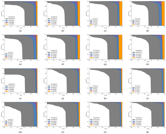
Figure 8.
Detailed PR curves for various oriented detectors on HRSID and RSDD-SAR. The legends of different colors in each figure represent the integral under the corresponding curve. The first two rows depict the PR curves on HRSID, while the last two rows display the PR curves on RSDD-SAR. (a–h) Our method, SSADet, ReDet, Roi-Transformer, Oriented RepPoints, FADet, FPDDet, and OEGR-DETR. (i–p) are similar to (a–h).
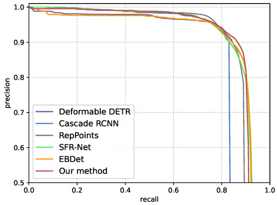
Figure 9.
PR curves of various detectors on SAR-Aircraft-v1.0.
4.4.1. Comparison Results on HRSID
Table 1 compares our proposed method with other detectors on HRSID. For accuracy measured by and , our method achieves 86.5% and 51.5%. Using the ResNet50 backbone, our method delivers the best results in these metrics among all single-model detectors. Specifically, compared to the state-of-art generic detectors, SKG-DDT outperforms Oriented RepPoints by 0.7% and 7.4%, ReDet by 2.1% and 0.2%, CFA by 1.9% and 11.1%, and Oriented RCNN by 5.6% and 8%. Compared to the state-of-art SAR-specific detectors, our method also outperforms FPDDet by 3.9% and 3.6%, FADet by 1.2% and 3.3%, OEGR-DETR by 1.4% and 2.7%, which are large margins. Additionally, our method achieves the second-best (58.4%) and the best (35.6%). These results highlight the excellent detection performance of our method for medium and large objects, though the performance diminishes slightly for small objects. Furthermore, our method achieves the highest precision (80.8%), surpassing the second-best detector by 6.3%, confirming its effectiveness in suppressing false alarms and improving the recognition accuracy.
The first two rows in Figure 8 present the PR curve analysis for various detectors on HRSID, where Figure 8a illustrates the analysis of our method. The effects of Loc, BG and FN can be observed as follows. First, the FN has a notable impact on our method. Replacing low IoU predictions with ground-truth boxes increases the AP by 4.0%. Second, the BG has a relatively minor effect, improving AP by 2.9% after removing FPs. Among these factors, Loc has the most significant impact. As indicated by the blue area, localization errors reduce the AP by 6.6%, which is higher than the effects of both BG and FN.
4.4.2. Comparison Results on RSDD-SAR
The comparison results on RSDD-SAR are also presented in Table 1. Unlike HRSID, RSDD-SAR contains relatively fewer objects per image. Despite this difference, our method achieves 92.7% and 46.3% , achieving the best among all detectors using the same ResNet50 backbone. Specifically, the proposed SKG-DDT outperforms ReDet by 0.7%, Oriented RepPoints by 5.8%, and Oriented RCNN by 3.7%. Compared to SAR-specific state-of-art detectors, our method also surpasses FPDDet by 0.6%, FADet by 1.8%, and OEGR-DETR by 1.6%. Additionally, our method achieves the highest precision (86.2%) on RSDD-SAR, outperforming the second-best detector by 1.4% with only a slight decrease in recall. While the detection performance for small objects remains less satisfactory, the method excels for medium and large objects, achieving the best results in (64.3%) and (95.0%).
The last two rows in Figure 8 illustrate the PR curve analysis for various detectors on RSDD-SAR. It can be observed that the Loc has the greatest impact on detection performance. Replacing low IoU predictions with ground-truth boxes increases the AP by 3.5%. The BG has the least impact, improving the AP by 1.8% after removing FPs (highlighted in the purple area). The missing detections decrease the AP by 2%, as shown in the orange area. The relatively lower performance for small objects is attributed to the sparse sampling strategy used in our method. However, the strengths of our method in detecting medium and large objects validate its effectiveness and robustness for scenarios with sparsely distributed objects.
4.4.3. Comparison Results on SAR-Aircraft-v1.0
The comparison results on SAR-Aircraft-v1.0 are summarized in Table 2. Compared to the state-of-art detectors based on HBB representation, our method achieves 89.2% and 63.7% . Using the same backbone of ResNet50, the proposed method achieves the best among all detectors using a single model without bells and whistles. Compared to generic detectors, our method outperforms Deformable DETR by 1.4%, Faster RCNN by 6.4%, Cascade RCNN by 7.5%, FCOS by 1.2%, RepPoints by 2.2%, and RetinaNet by 4.2%. Compared to SAR-specific state-of-art detectors, our method also outperforms SFR-Net by 1.1%, and EBDet by 1.0%. As expected, our method achieves the best results in precision, outperforming the second-best detector by 1%, which demonstrates its effectiveness in improving recognition accuracy and suppressing false alarms across diverse scenarios. Moreover, the proposed method excels in detecting medium and large aircraft, achieving 59.1% and 65.9% , outperforming the second-best detector by 1.0% and 1.5%, respectively.
4.5. Analysis of Visualization Results
The detection results of various oriented detectors on HRSID are visualized in Figure 10. To effectively highlight the advantages of our proposed method, we focus on two challenging scenarios: complex inshore scenes and densely distributed ship scenes. For state-of-art generic detectors, ReDet often misses densely packed inshore ships and produces a few false alarms in complex backgrounds. Although Oriented RepPoints achieves promising results across various metrics, it still generates false alarms in complex scenes and sometimes misclassifying multiple ships as a single one. Similarly, Oriented RCNN struggles with false alarms in inshore scenes and fails to detect certain closely packed ships. Using irregular quadrilaterals to represent object ourlines, Gliding Vertex performs poorly in complex scenes, being prone to both false alarms and missed detections. Overall, generic detectors struggle with complex scenarios, especially in detecting ships within densely packed or inshore environments. For state-of-art SAR detectors, FPDDet frequently suffers from false alarms and missed detections in nearshore regions. FADet shows noticeable improvements in suppressing false alarms but still misses ships near the shore. OG-BBAV underperforms significantly, particularly in detecting densely distributed ships. In contrast, our method demonstrates superior performance in detecting densely packed ships. Additionally, the specially designed SKFF module in our method effectively reduces false alarms, showcasing excellent anti-interference capabilities.
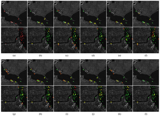
Figure 10.
The detection results of various oriented detectors on the HRSID. We choose a complex inshore scene and a densely distributed scene to thoroughly demonstrate the superior detection performance of the proposed method. The green rectangle, red rectangle, yellow circle, red circle, and orange circle correspond to detection results, ground truths, missing objects, false alarms, and low localization accuracy results, repectively. (a) Ground truth; (b) ReDet; (c) Roi-Transformer; (d) Oriented RepPoints; (e) CFA; (f) SSADet; (g) Oriented RCNN; (h) Gliding Vertex; (i) FPDDet; (j) OG-BBAV; (k) FADet; (l) our method.
The detection results of various detectors on RSDD-SAR are visualized in Figure 11. As in the previous analysis, we focus on two challenging scenarios: complex inshore scenes and densely distributed ship scenes. For state-of-art generic detectors, ReDet represents convincing results for densely packed ships, but false alarms persist in complex backgrounds. While free from false alarms, Oriented RepPoints misses a significant number of densely packed ships. Oriented RCNN demonstrates commendable detection performance for densely packed ships but tends to generate false alarms in complex scenes. For state-of-art SAR detectors, FPDDet achieves a high recall rate with minimal missing detections. However, it struggles with complex backgrounds, resulting in false alarms. Similarly, FADet successfully detects all ships but remains prone to generating false alarms in complex scenarios. OG-BBAV produces no false alarms but continues to miss densely arranged ships. In contrast, the proposed method demonstrates outstanding performance across various scenarios and shows robust resistance from complex backgrounds.
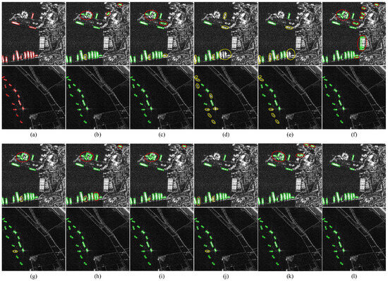
Figure 11.
Detection results of various oriented detectors on the RSDD-SAR. We choose a complex inshore scene and a densely distributed scene to thoroughly demonstrate the superior detection performance of the proposed method. The green rectangle, red rectangle, yellow circle, red circle, and orange circle correspond to detection results, ground truths, missing objects, false alarms, and low localization accuracy results, repectively. (a) Ground truth; (b) ReDet; (c) Roi-Transformer; (d) Oriented RepPoints; (e) CFA; (f) SSADet; (g) Oriented RCNN; (h) Gliding Vertex; (i) FPDDet; (j) OG-BBAV; (k) FADet; (l) our method.
The detection results of various detectors on SAR-Aircraft-v1.0 are visualized in Figure 12. The presence of occlusions and shadows diminishes the prominence of some aircraft in the image, introducing challenges in accurate recognition and localization. For representative generic detectors, Deformable DETR achieves excellent results in . However, it generates false alarms in background scattering regions and fails to detect less prominent aircraft. Cascade RCNN achieves higher precision with fewer false alarms, but it suffers from significant missing detections. RepPoints and RetinaNet show a higher rate of missing detection, particularly for aircraft located near airport terminals. For state-of-art SAR detectors, EBDet performs well with minimal false alarms but struggles to detect less conspicuous aircraft. In comparison, the proposed method has fewer missing detection and false alarms across various scenes, clearly demonstrating its superior performance in detecting less prominent aircraft and the effectiveness in suppressing false alarms.
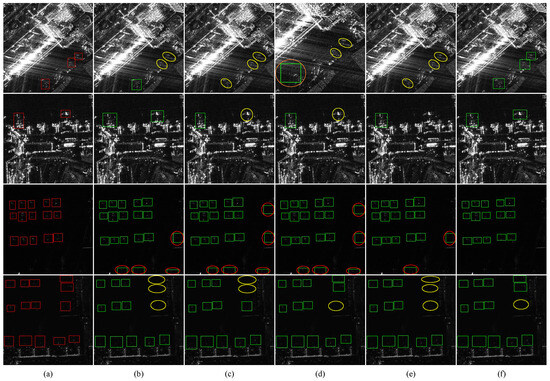
Figure 12.
Detection results on the SAR-Aircraft-v1.0. We choose the complex interference scene (first two rows) and the densely distributed scene (last two rows) to thoroughly demonstrate the superior performance of the proposed method. The green rectangle, red rectangle, yellow circle, red circle and orange circle correspond to detection results, ground truths, missing objects, false alarms and low localization accuracy results, respectively. (a) Ground truth; (b) Deformable DETR; (c) Cascade RCNN; (d) RepPoints; (e) EBDet; (f) our method.
4.6. Ablation Studies
This section presents a series of ablation experiments conducted on HRSID to evaluate the contribution of each component in our proposed method. We adopt Deformable DETR [40] with the OBB representation (Deformable DETR-O) as the . To ensure a fair comparison, all ablation experiments are conducted under identical conditions. The results of the ablation experiments are summarized in Table 3, with corresponding PR curves shown in Figure 13. As observed, each component of the proposed method contributes to an improvement in detection performance. Specifically, the and of the proposed method achieve 13.0% and 21.0% improvements compared with the . Moreover, the significant improvement of 73.2% in precision highlights the effectiveness of our method in enhancing recognition accuracy and reducing false alarms.
Table 3.
Ablation studies conducted on HRSID to evaluate the contributions of individual components in the proposed method. Bold values highlight the best performance.
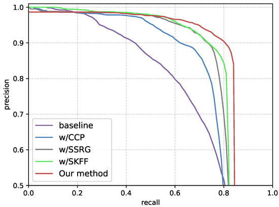
Figure 13.
PR curves of different advancements in the proposed method.
4.6.1. CCP Module Ablation Experiment
We first evaluate the effectiveness of the proposed CCP module by integrating it into . Specifically, we replace the regression branch of Deformable DETR with the CCP module, updating only the center-point coordinates of each query in the decoder. Furthermore, we set the in Equation (7) to the image’s width and height, while in Equation (6) represent the center-point coordinates of queries updated by the decoder. As shown in Table 3, incorporating the CCP module improves precision by 3.4% and by 2.4%. Figure 14 displays the predicted convex contours for ships and aircraft.
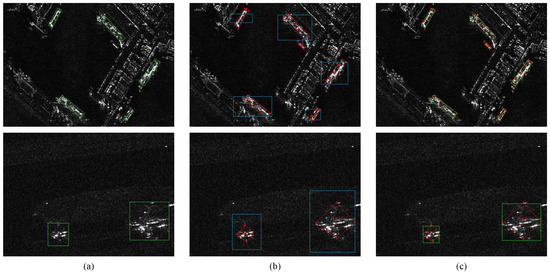
Figure 14.
The results of the predicted convex contour for ships and planes. (a) Ground truth. (b) The approximate object region, the predicted convex points, and the corresponding convex contour. (c) The convex contour and its minimal rectangle in OBBs (above) or HBBs (below). The green rectangle in (a) is the ground truth and in (c) is the minimal rectangle of the convex contour, the blue rectangle is the approximate object region generated by SSRG module, the red dots are convex points, and the red lines consist of the corresponding convex contour.
It is evident that the predicted fine-grained convex contour effectively delineates the object blurred outline. While this may be less noticeable for ships, which typically have regular shapes, it becomes particularly evident when dealing with aircraft that have irregular structures. Specifically, the predicted convex points accurately capture the head, tail, and wing sides of the aircraft. By integrating these essential structural keypoints, the CCP module constructs a polygon that tightly encloses the entire aircraft, outperforming traditional rectangular representations that fail to capture irregular structures accurately.
To analyze the impact of the hyperparameter , which controls the scale of the predicted offsets for convex points, we evaluate the model using various values (1.0, 1.2, 1.5, 1.8, and 2.0). The experimental results are shown in Table 4. It is noticeable that and other metrics achieve optimal when is set to 1.5. Deviating from this value, either by increasing or decreasing, leads to a noticeable decline in detection performance.
Table 4.
The ablation results for varying values in the CCP module, using the HRSID dataset. Bold values denote the best performance.
4.6.2. SSRG Module Ablation Experiment
The results in Table 3 demonstrate significant improvement when the SSRG and CCP modules are added to the , increasing precision by 57.4%, by 4.6%, and by 27.7%. This result highlights that detectors requiring dense sampling of candidates typically encounter significant challenges with false alarms in complex scenes, leading to reduced precision. By modeling the spatial distribution of strong scattering regions, the SSRG module effectively identifies approximate object regions. This approach eliminates a large portion of irrelevant background, enabling downstream processes to focus on the coarse object regions, thereby significantly improving accuracy and reducing false alarms. Moreover, the , , and metrics have also shown significant improvements of 11.9%, 14.9%, and 17.8%, demonstrating the SSRG module’s effectiveness across varying object scales. The blue rectangle in Figure 14 represents the approximate object regions obtained by the SSRG module.
Additionally, we perform detailed ablation studies on the three design variations of the denoising-decoder layer presented in Section 3.1.2, with the results summarized in Table 5. The findings indicate that design (c) yields the best performance across all metrics.
Table 5.
The ablation results of different denoising-decoder layer designs. HRSID is used in this experiment. The bold results indicate the best performance.
4.6.3. SKFF Module Ablation Experiment
Table 3 demonstrates the impact of integrating the SKFF module with the CCP module into the , resulting in precision improvements of 1.7%, a 5.4% increase in , and a 3.9% increase in . These improvements indicate that the SKFF module effectively captures the object structural information and the surrounding context, suppressing false alarms while enhancing the recognition and localization accuracy. In addition, the average precision for small, medium, and large objects is improved by 3.4%, 2.7% and 5.0%, respectively. Combining the SKFF and SSRG modules further amplifies performance gains, achieving superior results across all evaluation metrics. Additionally, the SKFF module addresses the recall-rate reduction introduced by the SSRG module by additionally preserving object structural and context information, resulting in a 3.6% recall improvement.
Figure 15 displays the scattering keypoints predicted by the SKFF module across multiple scales, demonstrating its ability to adaptively capture the object structural information. For instance, at small scales (0 and 1), scattering keypoints focus on specific object parts, while at large scales (2 and 3), they encompass the whole object. The results indicate that the predicted keypoints accurately capture critical scattering positions, validating the utility of the proposed multi-scale prediction approach.
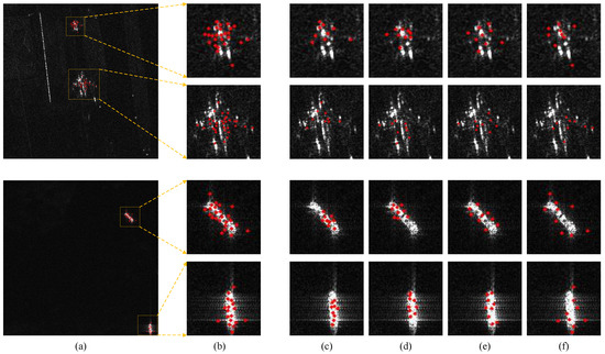
Figure 15.
The results of the predicted speckle and scattering keypoints in SKFF module. (a) The predicted scattering keypoints integrated from multiple feature levels. (b) The fused scattering keypoints of all feature levels. (c–f) The predicted keypoints of feature levels 0, 1, 2, and 3 respectively.
The hyperparameter K regulates the total number of scattering keypoints predicted at each scale for every object. To analyze its impact, we evaluate K values of 4, 9, 15, 20, and 25 while keeping other model components unchanged. The results presented in Table 6 reveal that all metrics reach their optimal values when K is set to 9. Generally, objects in SAR images exhibit multi-scale distribution. Smaller K values struggle to capture all scattering keypoints, particularly for large-scale objects, leading to suboptimal performance. Conversely, larger K values result in excessive clustering, especially for small objects, hindering the capture of structural and spatial relationships. Based on this analysis, we set K to 9, as this balances capturing structural information while minimizing overlap, yielding optimal results across all metrics.
Table 6.
The ablation results for different values of K in the SKFF module, using the HRSID dataset. Bold values highlight the best performance.
4.6.4. Number of Queries Ablation Experiment
The number of queries is an essential hyperparameter in the proposed method, as it directly affects the number of initialized noisy regions in the SSRG module. To evaluate its impact, we analyze the detection performance with different numbers of queries (100, 300, 500, 700, 900), illustrated in Figure 16. A higher query number leads to more predictions, notably boosting detection performance, though at the cost of increased training and testing durations. The findings reveal that starting from a lower query number, detection performance improves markedly with more queries, highlighting the critical role of adequately initialized queries. With only 100 queries, detection performance remains suboptimal, as and are limited to 64.9% and 34.5%, respectively. At 500 queries, detection performance peaks, with improving to 86.5% (a gain of 21.6%) and reaching 51.5% (an increase of 17.0%). However, increasing the number of queries to 700 and 900 leads to a small drop in detection performance, possibly due to the redundancy of queries interfering with the one-to-one matching process of the proposed method.
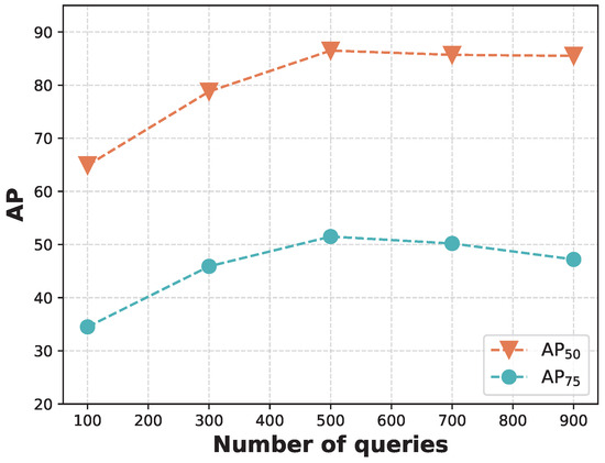
Figure 16.
The ablation results for different query numbers on the HRSID dataset. We compare the and with varying numbers of queries from 100 to 900.
5. Discussion
In this article, we propose a novel noise-to-convex paradigm with a hierarchical framework that effectively exploits the unique characteristics of SAR imagery alongside advanced deep learning techniques. By progressively refining object outlines from coarse regions to precise convex contours, our method addresses two critical challenges: blurred object outlines and increased false alarms in complex scenes. Extensive experiments on three public SAR datasets demonstrate the robustness and scalability of our approach.
Broader Applications. Although our design focuses on SAR oriented object detection, the underlying hierarchical strategy for handling blurred object outlines and false alarms can be readily adapted to other domains with equal challenges. A direct extension of our approach is SAR object detection under the HBB scenario, where experimental results confirm its effectiveness upon domain transfer. Moreover, radar and ultrasound imaging, where object edges are frequently obscured by noise, could similarly benefit from our noise-to-convex paradigm. By adapting the underlying scattering-keypoint features to diverse noise patterns, our method can serve as a robust, general-purpose detection solution beyond the SAR community.
Practical Value in Real-World Scenarios. From a practical standpoint, the proposed framework offers several advantages:
- Robustness to Noise. SAR imagery in maritime surveillance or disaster monitoring typically suffers from significant speckle noise and clutter, but our hierarchical approach effectively filters out irrelevant background regions to produce accurate detections with reduced false alarms.
- Reduced False Alarms. By leveraging geometric priors through adaptive scattering-keypoint detection and convex contour modeling, our method reduces the number of spurious detections, which is crucial for applications such as ship detection in congested sea lanes or vehicle recognition in complex urban environments.
- Adaptability to Varying Annotation Styles. Although our primary contribution focuses on oriented bounding boxes, the proposed method can be adapted to horizontal bounding boxes or other annotation formats with minimal changes, as demonstrated by experiments on the SAR-Aircraft-v1.0 dataset.
Collectively, these properties make the proposed noise-to-convex paradigm appealing for a wide range of real-world scenarios. By bridging the gap between abstract scattering signatures and precise object contours, the method can be deployed in both civilian and military SAR applications wherever accurate and robust target delineation is required.
Limitations and Future Work. Despite its superior performance, our method still encounters certain limitations under extreme conditions. First, detecting tiny objects remains challenging. Small targets often exhibit incomplete scattering-point clusters, and their scattering distributions are too sparse to reliably capture object geometry, leading to higher omission rates. Second, the computational overhead of the self-attention mechanism in the transformer-based detection head limits deployment in resource-constrained environments. Many edge devices or real-time systems lack the necessary hardware support for attention mechanisms, potentially hindering practical adoption. To address these issues, our future work will focus on several directions:
- Enhanced Tiny Object Detection. We plan to enhance the hierarchical design with multi-scale feature aggregation or context-aware attention strategies to better capture faint scattering signatures of very small objects.
- Model Optimization. We will investigate techniques such as model compression, knowledge distillation, and more efficient attention variants to facilitate easier deployment while maintaining detection accuracy. These optimizations will enhance the feasibility of our approach for on-board SAR processing and real-time surveillance.
- Exploration of Diffusion Models. Our experiments suggest that diffusion-based methods hold promise for enhancing both generative and discriminative capabilities in noisy SAR imagery. We plan to deeply integrate diffusion models with the underlying mechanisms of SAR imagery to further improve performance under severe clutter.
6. Conclusions
This article proposes a novel noise-to-convex detection paradigm with a hierarchical framework based on the SKG-DDT that integrates SAR-specific characteristics with advanced deep learning techniques. At the bottom level, the SSRG module leverages a diffusion model to learn the spatial distribution of scattering regions, enabling the direct generation of approximate object regions. At the middle level, the SKFF module dynamically detects scattering keypoints and captures their geometric and spatial relationships. At the top level, a fine-grained convex contour representation is obtained through the CCP module, providing detailed descriptions of blurred object outlines. These modules are seamlessly incorporated into a unified end-to-end pipeline via the detection transformer, achieving robust and accurate oriented object detection. Extensive experiments on the HRSID, RSDD-SAR, and SAR-Aircraft-v1.0 datasets demonstrate that the SKG-DDT outperforms existing state-of-the-art detectors across diverse scenarios.
Beyond its performance on benchmark datasets, the proposed method demonstrates significant practical value in real-world applications. Its adaptability to unclear object outlines and robustness to noise make it well-suited for tasks such as maritime surveillance, disaster monitoring, and urban traffic regulation. Furthermore, the capability of our framework to handle noisy or ambiguous object outlines makes it a promising candidate for other domains, such as radar and ultrasound imaging, where similar challenges arise. This highlights its broader applicability.
Despite its contributions, our method still faces challenges in detecting tiny objects, and its transformer-based architecture may limit deployment in resource-limited environments. In the future, we plan to enhance the detection performance for tiny objects by implementing advanced scattering feature extraction strategies. Additionally, we will optimize the model architecture to ensure seamless deployment across various hardware platforms. Furthermore, the integration of diffusion models will also be explored to enhance the method’s generative robustness and discriminative accuracy under severe noise conditions.
Author Contributions
Conceptualization, S.L. and C.H.; methodology, S.L. and M.T.; software, S.L.; validation, S.L.; formal analysis, S.L. and B.H.; investigation, S.L. and J.J.; resources, C.H.; data curation, S.L.; writing—original draft preparation, S.L.; writing—review and editing, S.L. and M.T.; visualization, S.L.; supervision, B.H.; project administration, J.J.; funding acquisition, C.H. All authors have read and agreed to the published version of the manuscript.
Funding
This research was funded by the National Key Research and Development Program of China (No. 2016YFC0803000) and the National Natural Science Foundation of China (No. 41371342).
Data Availability Statement
Data are contained within the article.
Acknowledgments
The authors would like to express their sincere gratitude to the editor and the anonymous reviewers for their valuable and constructive feedback, which have significantly contributed to enhancing the quality of this article.
Conflicts of Interest
The authors declare that they have no known competing financial interests or personal relationships that could have appeared to influence the work reported in this paper.
References
- Zhou, X.; Li, T. Ship detection in PolSAR images based on a modified polarimetric notch filter. Electronics 2023, 12, 2683. [Google Scholar] [CrossRef]
- Min-Woo, K.; Park, S.K.; Ju, J.G.; Noh, H.C.; Choi, D.G. Clean Collector Algorithm for Satellite Image Pre-Processing of SAR-to-EO Translation. Electronics 2024, 13, 4529. [Google Scholar] [CrossRef]
- Yang, C.; Wang, D.; Sun, F.; Wang, K. Maneuvering Trajectory Synthetic Aperture Radar Processing Based on the Decomposition of Transfer Functions in the Frequency Domain Using Average Blurred Edge Width Assessment. Electronics 2024, 13, 4100. [Google Scholar] [CrossRef]
- Sun, S.; Wang, J. Ship Detection in SAR Images Based on Steady CFAR Detector and Knowledge-Oriented GBDT Classifier. Electronics 2024, 13, 2692. [Google Scholar] [CrossRef]
- Zheng, H.; Xue, X.; Yue, R.; Liu, C.; Liu, Z. SAR Image Ship Target Detection Based on Receptive Field Enhancement Module and Cross-Layer Feature Fusion. Electronics 2023, 13, 167. [Google Scholar] [CrossRef]
- Gao, G.; Liu, L.; Zhao, L.; Shi, G.; Kuang, G. An adaptive and fast CFAR algorithm based on automatic censoring for target detection in high-resolution SAR images. IEEE Trans. Geosci. Remote Sens. 2008, 47, 1685–1697. [Google Scholar] [CrossRef]
- Li, Q.; Mou, L.; Liu, Q.; Wang, Y.; Zhu, X.X. HSF-Net: Multiscale deep feature embedding for ship detection in optical remote sensing imagery. IEEE Trans. Geosci. Remote Sens. 2018, 56, 7147–7161. [Google Scholar] [CrossRef]
- Nieto-Hidalgo, M.; Gallego, A.J.; Gil, P.; Pertusa, A. Two-stage convolutional neural network for ship and spill detection using SLAR images. IEEE Trans. Geosci. Remote Sens. 2018, 56, 5217–5230. [Google Scholar] [CrossRef]
- Du, L.; Li, L.; Wei, D.; Mao, J. Saliency-guided single shot multibox detector for target detection in SAR images. IEEE Trans. Geosci. Remote Sens. 2019, 58, 3366–3376. [Google Scholar] [CrossRef]
- Ai, J.; Tian, R.; Luo, Q.; Jin, J.; Tang, B. Multi-scale rotation-invariant Haar-like feature integrated CNN-based ship detection algorithm of multiple-target environment in SAR imagery. IEEE Trans. Geosci. Remote Sens. 2019, 57, 10070–10087. [Google Scholar] [CrossRef]
- Ren, S.; He, K.; Girshick, R.; Sun, J. Faster r-cnn: Towards real-time object detection with region proposal networks. IEEE Trans. Pattern Anal. Mach. Intell. 2017, 39, 1137–1149. [Google Scholar] [CrossRef]
- Redmon, J.; Divvala, S.; Girshick, R.; Farhadi, A. You only look once: Unified, real-time object detection. In Proceedings of the IEEE Conference on Computer Vision and Pattern Recognition, Las Vegas, NV, USA, 27–30 June 2016; pp. 779–788. [Google Scholar]
- Carion, N.; Massa, F.; Synnaeve, G.; Usunier, N.; Kirillov, A.; Zagoruyko, S. End-to-end object detection with transformers. In Proceedings of the European Conference on Computer Vision, Glasgow, UK, 23–28 August 2020; Springer: Berlin/Heidelberg, Germany, 2020; pp. 213–229. [Google Scholar]
- Wang, Z.; Du, L.; Mao, J.; Liu, B.; Yang, D. SAR target detection based on SSD with data augmentation and transfer learning. IEEE Geosci. Remote Sens. Lett. 2018, 16, 150–154. [Google Scholar] [CrossRef]
- Li, J.; Qu, C.; Shao, J. Ship detection in SAR images based on an improved faster R-CNN. In Proceedings of the IEEE 2017 SAR in Big Data Era: Models, Methods and Applications (BIGSARDATA), Beijing, China, 13–14 November 2017; pp. 1–6. [Google Scholar]
- Jiao, J.; Zhang, Y.; Sun, H.; Yang, X.; Gao, X.; Hong, W.; Fu, K.; Sun, X. A densely connected end-to-end neural network for multiscale and multiscene SAR ship detection. IEEE Access 2018, 6, 20881–20892. [Google Scholar] [CrossRef]
- An, Q.; Pan, Z.; Liu, L.; You, H. DRBox-v2: An improved detector with rotatable boxes for target detection in SAR images. IEEE Trans. Geosci. Remote Sens. 2019, 57, 8333–8349. [Google Scholar] [CrossRef]
- Sun, Y.; Wang, Z.; Sun, X.; Fu, K. SPAN: Strong scattering point aware network for ship detection and classification in large-scale SAR imagery. IEEE J. Sel. Top. Appl. Earth Obs. Remote Sens. 2022, 15, 1188–1204. [Google Scholar] [CrossRef]
- Zhang, C.; Yang, C.; Cheng, K.; Guan, N.; Dong, H.; Deng, B. MSIF: Multisize inference fusion-based false alarm elimination for ship detection in large-scale SAR images. IEEE Trans. Geosci. Remote Sens. 2022, 60, 1–11. [Google Scholar] [CrossRef]
- Cui, Z.; Li, Q.; Cao, Z.; Liu, N. Dense attention pyramid networks for multi-scale ship detection in SAR images. IEEE Trans. Geosci. Remote Sens. 2019, 57, 8983–8997. [Google Scholar] [CrossRef]
- Kang, Y.; Wang, Z.; Fu, J.; Sun, X.; Fu, K. SFR-Net: Scattering feature relation network for aircraft detection in complex SAR images. IEEE Trans. Geosci. Remote Sens. 2021, 60, 1–17. [Google Scholar] [CrossRef]
- Yang, X.; Zhang, X.; Wang, N.; Gao, X. A robust one-stage detector for multiscale ship detection with complex background in massive SAR images. IEEE Trans. Geosci. Remote Sens. 2021, 60, 1–12. [Google Scholar] [CrossRef]
- Sun, Y.; Sun, X.; Wang, Z.; Fu, K. Oriented ship detection based on strong scattering points network in large-scale SAR images. IEEE Trans. Geosci. Remote Sens. 2021, 60, 1–18. [Google Scholar] [CrossRef]
- Guo, P.; Celik, T.; Liu, N.; Li, H.C. Break through the border restriction of horizontal bounding box for arbitrary-oriented ship detection in SAR images. IEEE Geosci. Remote Sens. Lett. 2023, 20, 1–5. [Google Scholar] [CrossRef]
- Zhao, Y.; Zhao, L.; Liu, Z.; Hu, D.; Kuang, G.; Liu, L. Attentional feature refinement and alignment network for aircraft detection in SAR imagery. arXiv 2022, arXiv:2201.07124. [Google Scholar] [CrossRef]
- Fu, K.; Fu, J.; Wang, Z.; Sun, X. Scattering-keypoint-guided network for oriented ship detection in high-resolution and large-scale SAR images. IEEE J. Sel. Top. Appl. Earth Obs. Remote Sens. 2021, 14, 11162–11178. [Google Scholar] [CrossRef]
- Pan, D.; Gao, X.; Dai, W.; Fu, J.; Wang, Z.; Sun, X.; Wu, Y. SRT-Net: Scattering region topology network for oriented ship detection in large-scale SAR images. IEEE Trans. Geosci. Remote. Sens. 2024, 62, 5202318. [Google Scholar] [CrossRef]
- Ju, M.; Niu, B.; Zhang, J. FPDDet: An Efficient Rotated SAR Ship Detector Based on Simple Polar Encoding and Decoding. IEEE Trans. Geosci. Remote. Sens. 2023, 61, 5218915. [Google Scholar] [CrossRef]
- Wan, H.; Chen, J.; Huang, Z.; Du, W.; Xu, F.; Wang, F.; Wu, B. Orientation Detector for Small Ship Targets in SAR Images Based on Semantic Flow Feature Alignment and Gaussian Label Matching. IEEE Trans. Geosci. Remote. Sens. 2023, 61, 5218616. [Google Scholar] [CrossRef]
- Kang, M.; Ji, K.; Leng, X.; Lin, Z. Contextual region-based convolutional neural network with multilayer fusion for SAR ship detection. Remote Sens. 2017, 9, 860. [Google Scholar] [CrossRef]
- Chen, C.; He, C.; Hu, C.; Pei, H.; Jiao, L. MSARN: A deep neural network based on an adaptive recalibration mechanism for multiscale and arbitrary-oriented SAR ship detection. IEEE Access 2019, 7, 159262–159283. [Google Scholar] [CrossRef]
- Fu, K.; Dou, F.Z.; Li, H.C.; Diao, W.H.; Sun, X.; Xu, G.L. Aircraft recognition in SAR images based on scattering structure feature and template matching. IEEE J. Sel. Top. Appl. Earth Obs. Remote Sens. 2018, 11, 4206–4217. [Google Scholar] [CrossRef]
- Ho, J.; Jain, A.; Abbeel, P. Denoising diffusion probabilistic models. Adv. Neural Inf. Process. Syst. 2020, 33, 6840–6851. [Google Scholar]
- Song, J.; Meng, C.; Ermon, S. Denoising diffusion implicit models. arXiv 2020, arXiv:2010.02502. [Google Scholar]
- Takagi, Y.; Nishimoto, S. High-resolution image reconstruction with latent diffusion models from human brain activity. In Proceedings of the IEEE/CVF Conference on Computer Vision and Pattern Recognition, Vancouver, BC, Canada, 18–22 June 2023; pp. 14453–14463. [Google Scholar]
- Gu, Z.; Chen, H.; Xu, Z. Diffusioninst: Diffusion model for instance segmentation. In Proceedings of the ICASSP 2024-2024 IEEE International Conference on Acoustics, Speech and Signal Processing (ICASSP), Seoul, Republic of Korea, 14–19 April 2024; pp. 2730–2734. [Google Scholar]
- Chen, S.; Sun, P.; Song, Y.; Luo, P. Diffusiondet: Diffusion model for object detection. In Proceedings of the IEEE/CVF International Conference on Computer Vision, Paris, France, 2–6 October 2023; pp. 19830–19843. [Google Scholar]
- Perera, M.V.; Nair, N.G.; Bandara, W.G.C.; Patel, V.M. SAR despeckling using a denoising diffusion probabilistic model. IEEE Geosci. Remote Sens. Lett. 2023, 20, 1–5. [Google Scholar] [CrossRef]
- Zhang, X.; Li, Y.; Li, F.; Jiang, H.; Wang, Y.; Zhang, L.; Zheng, L.; Ding, Z. Ship-Go: SAR ship images inpainting via instance-to-image generative diffusion models. ISPRS J. Photogramm. Remote Sens. 2024, 207, 203–217. [Google Scholar] [CrossRef]
- Zhu, X.; Su, W.; Lu, L.; Li, B.; Wang, X.; Dai, J. Deformable detr: Deformable transformers for end-to-end object detection. arXiv 2020, arXiv:2010.04159. [Google Scholar]
- Song, Y.; Ermon, S. Improved techniques for training score-based generative models. Adv. Neural Inf. Process. Syst. 2020, 33, 12438–12448. [Google Scholar]
- Perez, E.; Strub, F.; De Vries, H.; Dumoulin, V.; Courville, A. Film: Visual reasoning with a general conditioning layer. In Proceedings of the AAAI Conference on Artificial Intelligence, New Orleans, LA, USA, 2–7 February 2018; Volume 32, pp. 3942–3951. [Google Scholar]
- Guo, Q.; Wang, H.; Xu, F. Scattering enhanced attention pyramid network for aircraft detection in SAR images. IEEE Trans. Geosci. Remote Sens. 2020, 59, 7570–7587. [Google Scholar] [CrossRef]
- Guo, Z.; Liu, C.; Zhang, X.; Jiao, J.; Ji, X.; Ye, Q. Beyond bounding-box: Convex-hull feature adaptation for oriented and densely packed object detection. In Proceedings of the IEEE/CVF Conference on Computer Vision and Pattern Recognition, Nashville, TN, USA, 20–25 June 2021; pp. 8792–8801. [Google Scholar]
- Jarvis, R.A. On the identification of the convex hull of a finite set of points in the plane. Inf. Process. Lett. 1973, 2, 18–21. [Google Scholar] [CrossRef]
- Lin, T.Y.; Goyal, P.; Girshick, R.; He, K.; Dollár, P. Focal loss for dense object detection. In Proceedings of the IEEE International Conference on Computer Vision, Venice, Italy, 22–29 October 2017; pp. 2980–2988. [Google Scholar]
- Wei, S.; Zeng, X.; Qu, Q.; Wang, M.; Su, H.; Shi, J. HRSID: A high-resolution SAR images dataset for ship detection and instance segmentation. IEEE Access 2020, 8, 120234–120254. [Google Scholar] [CrossRef]
- Congan, X.; Hang, S.; Jianwei, L.; Yu, L.; Libo, Y.; Long, G.; Wenjun, Y.; Taoyang, W. RSDD-SAR: Rotated ship detection dataset in SAR images. J. Radars 2022, 11, 581–599. [Google Scholar]
- Zhirui, W.; Yuzhuo, K.; Xuan, Z.; Yuelei, W.; Ting, Z.; Xian, S. SAR-AIRcraft-1.0: High-resolution SAR aircraft detection and recognition dataset. J. Radars 2023, 12, 906–922. [Google Scholar]
- Zhou, Y.; Yang, X.; Zhang, G.; Wang, J.; Liu, Y.; Hou, L.; Jiang, X.; Liu, X.; Yan, J.; Lyu, C.; et al. Mmrotate: A rotated object detection benchmark using pytorch. In Proceedings of the 30th ACM International Conference on Multimedia, Lisbon, Portugal, 10–14 October 2022; pp. 7331–7334. [Google Scholar]
- He, K.; Zhang, X.; Ren, S.; Sun, J. Deep residual learning for image recognition. In Proceedings of the IEEE Conference on Computer Vision and Pattern Recognition, Las Vegas, NV, USA, 27–30 June 2016; pp. 770–778. [Google Scholar]
- Deng, J.; Dong, W.; Socher, R.; Li, L.J.; Li, K.; Fei-Fei, L. Imagenet: A large-scale hierarchical image database. In Proceedings of the 2009 IEEE Conference on Computer Vision and Pattern Recognition, Miami, FL, USA, 20–25 June 2009; pp. 248–255. [Google Scholar]
- Lin, T.Y.; Maire, M.; Belongie, S.; Hays, J.; Perona, P.; Ramanan, D.; Dollár, P.; Zitnick, C.L. Microsoft coco: Common objects in context. In Proceedings of the Computer Vision–ECCV 2014: 13th European Conference, Zurich, Switzerland, 6–12 September 2014; Proceedings, Part V 13. Springer: Berlin/Heidelberg, Germany, 2014; pp. 740–755. [Google Scholar]
- Li, W.; Chen, Y.; Hu, K.; Zhu, J. Oriented reppoints for aerial object detection. In Proceedings of the IEEE/CVF Conference on Computer Vision and Pattern Recognition, New Orleans, LA, USA, 18–24 June 2022; pp. 1829–1838. [Google Scholar]
- Xie, X.; Cheng, G.; Wang, J.; Yao, X.; Han, J. Oriented R-CNN for object detection. In Proceedings of the IEEE/CVF International Conference on Computer Vision, Montreal, BC, Canada, 11–17 October 2021; pp. 3520–3529. [Google Scholar]
- Zhu, J.; Jing, D.; Gao, D. Stage-by-Stage Adaptive Alignment Mechanism for Object Detection in Aerial Images. Electronics 2024, 13, 3640. [Google Scholar] [CrossRef]
- Xia, G.S.; Bai, X.; Ding, J.; Zhu, Z.; Belongie, S.; Luo, J.; Datcu, M.; Pelillo, M.; Zhang, L. DOTA: A large-scale dataset for object detection in aerial images. In Proceedings of the IEEE Conference on Computer Vision and Pattern Recognition, Salt Lake City, UT, USA, 18–22 June 2018; pp. 3974–3983. [Google Scholar]
- Dai, L.; Liu, H.; Tang, H.; Wu, Z.; Song, P. Ao2-detr: Arbitrary-oriented object detection transformer. IEEE Trans. Circuits Syst. Video Technol. 2022, 33, 2342–2356. [Google Scholar] [CrossRef]
- Tian, Z.; Shen, C.; Chen, H.; He, T. Fcos: Fully convolutional one-stage object detection. In Proceedings of the IEEE/CVF International Conference on Computer Vision, Seoul, Republic of Korea, 27 October–2 November 2019; pp. 9627–9636. [Google Scholar]
- Xu, Y.; Fu, M.; Wang, Q.; Wang, Y.; Chen, K.; Xia, G.S.; Bai, X. Gliding vertex on the horizontal bounding box for multi-oriented object detection. IEEE Trans. Pattern Anal. Mach. Intell. 2020, 43, 1452–1459. [Google Scholar] [CrossRef] [PubMed]
- Feng, Y.; You, Y.; Tian, J.; Meng, G. OEGR-DETR: A Novel Detection Transformer Based on Orientation Enhancement and Group Relations for SAR Object Detection. Remote Sens. 2023, 16, 106. [Google Scholar] [CrossRef]
- Zhang, J.; Xing, M.; Sun, G.C.; Li, N. Oriented Gaussian function-based box boundary-aware vectors for oriented ship detection in multiresolution SAR imagery. IEEE Trans. Geosci. Remote Sens. 2021, 60, 1–15. [Google Scholar] [CrossRef]
- Cai, Z.; Vasconcelos, N. Cascade r-cnn: Delving into high quality object detection. In Proceedings of the IEEE Conference on Computer Vision and Pattern Recognition, Salt Lake City, UT, USA, 18–22 June 2018; pp. 6154–6162. [Google Scholar]
- Yang, Z.; Liu, S.; Hu, H.; Wang, L.; Lin, S. Reppoints: Point set representation for object detection. In Proceedings of the IEEE/CVF International Conference on Computer Vision, Seoul, Republic of Korea, 27 October–2 November 2019; pp. 9657–9666. [Google Scholar]
- Zhang, C.Q.; Deng, Y.; Chong, M.Z.; Zhang, Z.W.; Tan, Y.H. Entropy-Based re-sampling method on SAR class imbalance target detection. ISPRS J. Photogramm. Remote Sens. 2024, 209, 432–447. [Google Scholar] [CrossRef]
Disclaimer/Publisher’s Note: The statements, opinions and data contained in all publications are solely those of the individual author(s) and contributor(s) and not of MDPI and/or the editor(s). MDPI and/or the editor(s) disclaim responsibility for any injury to people or property resulting from any ideas, methods, instructions or products referred to in the content. |
© 2025 by the authors. Licensee MDPI, Basel, Switzerland. This article is an open access article distributed under the terms and conditions of the Creative Commons Attribution (CC BY) license (https://creativecommons.org/licenses/by/4.0/).