Design of Self-Optimizing Polynomial Neural Networks with Temporal Feature Enhancement for Time Series Classification

Abstract

Time series classification is a significant and complex issue in data mining, it is prevalent across various fields and holds substantial research value. However, enhancing the classification rate of time series data remains a formidable challenge. Traditional time series classification methods often face difficulties related to insufficient feature extraction or excessive model complexity. In this study, we propose a self-optimizing polynomial neural network with a temporal feature enhancement, which is referred to as OPNN-T. Existing classifiers based on polynomial neural networks (PNNs) struggle to achieve high-quality performances when dealing with time series data, primarily due to their inability to extract temporal information effectively. The goal of the proposed classifier is to enhance the nonlinear modeling capability for time series data, thereby improving the classification rate in practical applications. The key features of the proposed OPNN-T include the following: (1) A temporal feature module is employed to capture the dependencies in time series data, providing adaptability and flexibility in handling complex temporal patterns. (2) A polynomial neural network (PNN) is constructed using sub-datasets combined with three types of polynomial neurons, which enhances its nonlinear modeling capabilities across diverse scenarios. (3) A self-optimization mechanism is integrated into iteratively optimized sub-datasets, features, and polynomial types, resulting in significant improvements in the classification rate. The experimental results demonstrate that the proposed method achieves superior performances across multiple standard time series datasets, exhibiting higher classification accuracy and greater robustness than the existing classification models. Our research offers an effective solution for time series classification, and highlights the potential of polynomial neural networks in this field.

1. Introduction

Machine learning-based classifiers have been successfully applied across various fields, and time series classification is a significant research area that has garnered increasing attention [1,2]. Numerous practical solutions rely on time series classification techniques, such as medical diagnosis [3], seismic wave analysis [4], road condition monitoring [5], and anomaly detection [6]. These applications have accelerated the rapid development of time series classification research. However, time series data are characterized by high data volumes, significant noise, and unknown spans of temporal dependencies [7]. Additionally, since time series data consist of continuous numerical sequences, extracting effective features from the raw sequences poses a considerable challenge. The complexity of the classification tasks [8] and the ever-increasing scale of the data [9] further exacerbates the difficulties in achieving accurate and efficient time series classification.

Researchers have proposed various techniques for implementing classifiers, including methods such as K-nearest neighbor (KNN) [10], support vector machines (SVMS) [11,12], naive Bayes [13], and decision trees [14]. The classifiers achieve classification by learning the fundamental features of each class, making the construction of classifiers closely linked to the nature of the samples. In time series classification, a variety of methods for feature extraction are typically employed in either the time domain or the frequency domain to map the original time series into a lower-dimensional feature space. This approach offers notable advantages. First, feature extraction effectively captures the essential characteristics of the original time series, which can significantly improve the accuracy of the classifier in most cases. Second, these methods often exhibit an inherent noise reduction capability, allowing them to filter out some of the noise present in the raw data. Finally, processing data points in a lower-dimensional feature space is more resource-efficient, saving both computational power and time. Therefore, the properties demonstrated by the feature extraction methods, such as dimensionality reduction and noise resilience, provide robust support for developing high-performance classifiers.

Neural networks [15,16] have opened new possibilities for machine learning and pattern recognition, showcasing their unique advantages such as their learning capabilities, generalization abilities, and robustness. Among them, the earliest neural network classifier was the well-known multilayer perceptron (MLP) [17]. Researchers have subsequently introduced various neural network classifiers, including backpropagation (BP) neural networks [18], radial basis function neural networks (RBFNNs) [19] and polynomial neural networks (PNNs) [20]. Although these classifiers have made significant advances, there is substantial room for improvement in the context of time series classification, particularly in addressing the complexity of temporal dependencies, nonlinear patterns, and high dimensionalities in time series data. Real-world applications, such as anomaly detection in industrial equipment, financial forecasting, and health care monitoring, all require efficient and accurate time series classification models. However, the existing methods often struggle to achieve satisfactory performances due to their limitations in capturing intricate temporal relationships or adapting to diverse application scenarios. For instance, in healthcare, the accurate classification of time series data, such as electrocardiogram (ECG) signals, is critical for diagnosing heart conditions. Similarly, in industrial contexts, identifying irregular temporal patterns in sensor data can prevent equipment failure and reduce downtime. These challenges highlight the need for novel models that can effectively address these issues with improved accuracy and robustness.

In recent years, scholars have proposed several effective classification models specifically for time series data. For instance, TBOPE [21] integrates multiple TBOP single classifiers, combining sample averages and trend features for classification. RSFCF [22] reduces the search space by using randomly selected shapelets and embedding multiple typical time series features in the shapelet transformation, thus enhancing the model’s adaptability. AFFNet [23] improves the classification rate by adaptively fusing the multiscale temporal features and distance features of the time series data. These innovations reflect an ongoing effort to enhance the performance of classifiers in the challenging domain of time series classification.

The performance of recurrent neural networks (RNNs) [24] in time series forecasting has inspired us to explore a fusion in classification tasks. RNN is a class of deep learning algorithms commonly employed for modeling sequential data that are temporally correlated. Long short-term memory (LSTM) networks can be considered specialized extensions of RNNs, which are designed to address the shortcomings of traditional RNNs in capturing complicated dependencies. Consequently, employing LSTM networks as the primary component of the temporal feature module significantly enhances the model’s adaptability to time series features. We chose PNN as our research object due to its ability to model complex nonlinear relationships and its inherent advantages in function approximation. This combination aims to leverage LSTM’s strength in sequential data processing while benefiting from the expressive power of PNNs, which could potentially lead to an improved classification rate.

The integration of LSTM and PNN provides complementary strengths that address the limitations inherent in each individual approach. LSTM networks specialize in learning temporal dependencies by leveraging memory cells and gating mechanisms, which allows them to retain the relevant temporal information and discard the irrelevant details. This makes them exceptionally effective at capturing the sequential patterns, trends, and dependencies in time series data. However, while LSTM excels at extracting temporal features, it is not explicitly designed to model the complex nonlinear interactions between the features, which are often critical for classification tasks. PNNs, on the other hand, are particularly effective for representing nonlinear relationships through their polynomial-based structure, which approximates complex functions by combining low-order and high-order terms. When applied to the temporal features extracted by LSTM, PNNs enhance the model’s ability to capture intricate feature relationships and construct nonlinear decision boundaries. This interaction ensures that the information extracted from the sequential data is effectively utilized for classification, allowing the combined framework to address both the temporal and nonlinear complexities in the data.

We also observed that employing various optimization algorithms within neural network models can significantly enhance their performance. Numerous optimized neural network classifiers have been developed, including optimized radial basis function neural networks [25,26], among others. Particle swarm optimization (PSO) [27], as a global optimization algorithm grounded in swarm intelligence, has garnered significant attention due to its superiority in addressing complex optimization problems. By simulating the collaborative behavior of biological populations, PSO effectively achieves a balance between global exploration and local exploitation. Compared with other optimization algorithms, PSO is characterized by its simplicity and ease of use, requiring minimal parameter tuning and exhibiting a reduced risk of overfitting. This makes it especially suitable for optimizing neural networks. Therefore, we adopted the PSO algorithm as our primary self-optimizing technique, leading to improved performances in complex scenarios.

This study introduces a novel self-optimizing polynomial neural network with temporal feature enhancement (OPNN-T) for time series classification. The main features of OPNN-T are as follows: First, OPNN-T uses a temporal enhancement module for feature extraction from time series data. Compared with other statistical methods such as principal component analysis (PCA), the temporal enhancement module has the advantage of being able to capture the temporal features of samples, making it more suitable for time series data. Second, OPNN-T constructs a polynomial neural network classifier (PNNC) via sub-datasets and three types of polynomial neurons, employing least squares estimation (LSE) [28,29] to converge on the parameters. The combination of various polynomial types effectively enhances the representational capacity of the classifier, compared to using separate linear or quadratic polynomials. Finally, to improve the model’s adaptability across different scenarios and reduce overfitting to training data, we optimize the combination of polynomial types and subsets via the self-optimization strategy.

The remainder of this paper is structured as follows: Section 2 presents the main architecture of self-optimizing polynomial neural networks with temporal feature enhancement. Section 3 discusses the learning and optimization methods for OPNN-T. Section 4 provides experimental results and an analysis, demonstrating the feasibility and superiority of our model for time series classification. Finally, Section 5 concludes the paper and offers future perspectives.

2. Architecture Design of the Proposed Model

The architecture of the OPNN-T consists of three main modules: temporal feature enhancement, polynomial neural network classifiers, and self-optimization strategy. The temporal feature enhancement module is designed to capture the time series feature information of the sequences, effectively extracting the dynamic changes and correlations inherent in the time series data. The PNNC is constructed via three different types of polynomials, ensuring the classifier’s flexibility in representing complex decision boundaries. The coefficients of the polynomial functions are estimated via LSE, while the self-optimizing strategy is employed to optimize the model parameters. This approach facilitates the convergence of the model while enhancing the classification performance. Finally, by combining binary classifiers with a discriminative function, the model can obtain classification results efficiently, thereby effectively accomplishing the time series classification task.

2.1. Structure of Temporal Feature Enhancement Module

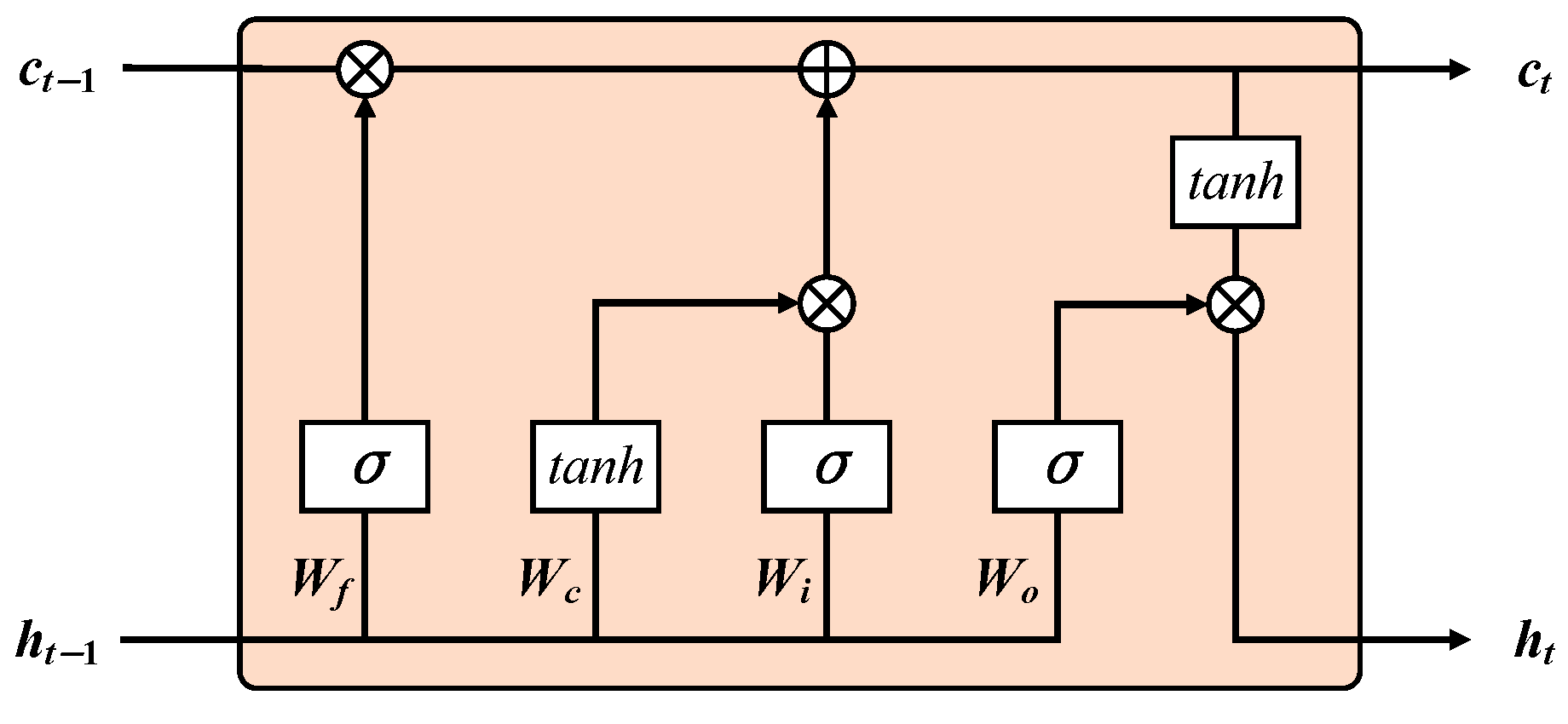
As a fundamental component of the temporal feature enhancement module, an LSTM network is an improved variant of an RNN that can recognize nonlinear patterns in data and retain historical information over longer time steps. In our model, the LSTM is designed with 128 hidden layer nodes, which provides sufficient capacity to model the complex temporal dependencies in the data without introducing unnecessary computational complexity. Additionally, the output layer consists of 16 nodes, which are determined based on the specific requirements of the task. This balance ensures that the model remains efficient when achieving high predictive accuracy.

The unique memory and gating mechanisms of LSTM, combined with the use of nonlinear activation functions in each layer, make it well-suited for learning long-term dependencies. The cell state of the LSTM is responsible for the transmission of information, which is central to its functionality. A key feature of LSTM is the design of three types of gates: the input gate, the forget gate, and the output gate, as illustrated in Figure 1. These gates are specifically designed to effectively protect and manage the cell state.

Let $\left\{x_1,x_2,\dots ,x_T\right\}$ be a typical input sequence for the LSTM, where $x_t\in R^k$ represents a k-dimensional real-valued vector at time step t. The function of the forget gate is to determine which information should be discarded from the cell state. Its operation can be described as follows:

$$f_t=\sigma (W_f\times x_t+U_f\times h_{t-1}+b_f)$$

(1)

where $f_t$ represents the forget threshold, and $\sigma$ denotes the sigmoid activation function, which transforms input values into a range between 0 and 1. The input values are denoted as $x_t$, $W_f$ represents the input weights, $U_f$ refers to the recurrent weights, $h_{t-1}$ is the output value at time step $t-1$, and $b_f$ is the bias term. The function of the input gate is to determine which pieces of information will be stored in the cell state.

$$i_t=\sigma (W_i\times x_t+U_i\times h_{t-1}+b_i)$$

(2)

$$\overline{C_t}=tanh(W_c\times x_t+U_c\times h_{t-1}+b_c)$$

(3)

where $i_t$ represents the input threshold, $W_i$ and $W_c$ are the corresponding input weights, and $U_i$ and $U_c$ are recurrent weights. $b_i$ and $b_c$ denote the bias term. Equation (4) is utilized to update the cell state at time step t, where $C_{t-1}$ represents the memory content at time step $t-1$.

$$C_t=f_t\times C_{t-1}+i_t\times \overline{C_t}$$

(4)

Output Gate: This gate is responsible for generating the output information, which can be described as follows:

$$O_t=\sigma (W_o\times x_t+U_o\times h_{t-1}+b_o)$$

(5)

where $O_t$ represents the output threshold at time step t, $W_o$ denotes the input weights, $U_o$ refers to the recurrent weights, and $b_o$ is the bias term. The output value at time step t can be expressed as follows:

$$h_t=O_t\times tanh{C}_t$$

(6)

The cell state is processed through the tanh function to normalize the values between −1 and 1, and then it is multiplied by $O_t$. $C_t$ represents the cell state at time step t. The values of W, U, and b are all determined through the learning process during training. The gated structure of the LSTM enables it to effectively capture both the short-term and long-term temporal dependencies within the sequence.

2.2. Structure of the Polynomial Neural Network Classifier

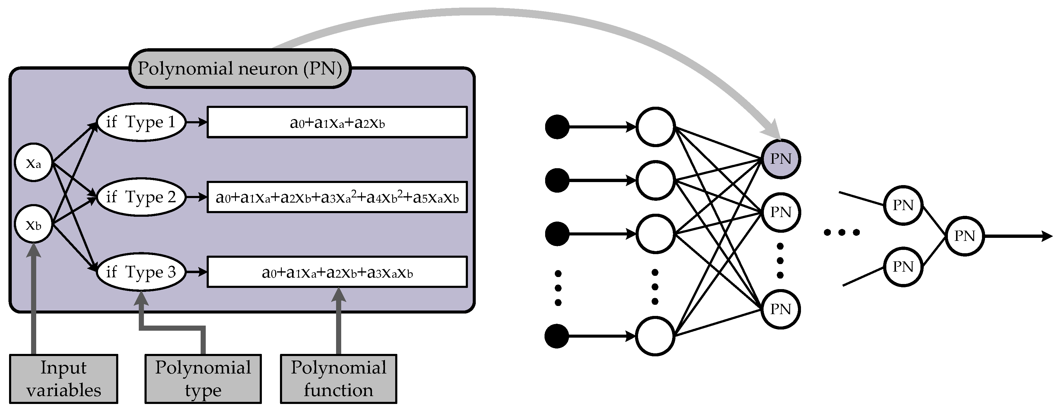
Polynomials are utilized to estimate the multivariate higher-order relationships between inputs and outputs. In this paper, we construct a polynomial neural network classifiers using the following three types of polynomials:

Linear polynomials (Type 1):

$$f_j=a_{j0}+a_{j1}{x}_1+\dots +a_{jk}{x}_k$$

(7)

Quadratic polynomials (Type 2):

$$f_j=a_{j0}+a_{j1}{x}_1+\dots +a_{jk}{x}_k+a_{j(k+1)}{x}_1^2+\dots +a_{j\left(2k\right)}{x}_k^2+a_{j(2k+1)}{x}_1{x}_2+\dots +a_{j\left(\right(k+2\left)\right(k+1)/2)}{x}_{k-1}{x}_k$$

(8)

Modified quadratic polynomials (Type 3):

$$f_j=a_{j0}+a_{j1}{x}_1+\dots +a_{jk}{x}_k+a_{j(k+1)}{x}_1{x}_2+\dots +a_{j\left(\right(k+2\left)\right(k+1)/2)}{x}_{k-1}{x}_k$$

(9)

In these expressions, the coefficients of the polynomials are represented as $a_{jn}$ for each $n=0,1,\dots ,k$. Meanwhile, $x_k$ denotes the input variables, and y signifies the output data.

Figure 2 illustrates the basic structure of polynomial neurons and polynomial neural networks. In this figure, PN denotes the type of neurons, where $x_a$ and $x_b$ represent the input variables, $a_0,a_1,a_2$ and $a_3$ indicate the coefficients of the polynomials.

2.3. Structure of the Sub-Dataset Generator

Inspired by the random forest (RF) algorithm, we constructed a sub-dataset generator using two components, as illustrated in Figure 3. In the first component, random sampling is employed to handle the rows of the data, where M random sub-samples are obtained. The second component processes the columns of the data, using information gain (IG) [30] to evaluate the importance of each feature. The feature with the highest information gain is selected as the decision feature in the decision tree, as shown in the figure.

The IG quantifies how much information a feature contributes to the classification system. The greater the amount of information provided by a feature, the greater its importance. For a variable X with m possible values, each with a probability $p\left(x_i\right)$, the entropy of X is defined as follows:

$$H\left(X\right)=-\sum _{i=0}^{m}p\left(x_i\right)logp\left(x_i\right)$$

(10)

The greater the number of possible values for X, the more information there is, and the higher entropy it carries. In the case of multi-feature classification, the IG for a feature is calculated by subtracting the conditional entropy, given the known features, from the original entropy. Consequently, the IG contributed by feature N with respect to class C is expressed as follows:

$$IG\left(\mathrm{N}\right)=H\left(C\right)-H\left(C\right|N)$$

(11)

Features are then ranked in descending order based on their IG to create a new feature sequence. From this new sequence, n features are selected and input into the training model. Generally, $n\le N$, where N represents the total number of features in the original dataset.

2.4. Structure of OPNN-T

The OPNN-T comprises two distinct types of neural networks: long short-term memory networks, which are based on deep learning methods, and polynomial neural networks. The proposed OPNN-T architecture is illustrated in Figure 4, where the temporal feature enhancement module is designed to capture the temporal features of time series data. The PNNC is employed to flexibly approximate the relationship between inputs and outputs and to capture the inherent uncertainties within the data. A generator produces sub-datasets of varying sizes and feature quantities, self-optimizing the dataset size, features, and polynomial types.

3. Learning Techniques of OPNN-T

In the proposed model, the time backpropagation algorithm is employed for learning the parameters of the LSTM layers in the temporal feature enhancement module. This algorithm serves as the core method for training LSTM layers and effectively captures both the long-term and short-term features present in time series data. The PNNC utilizes least squares estimation to adjust the weights. To enable the model’s key parameters to flexibly adapt to different datasets, the particle swarm algorithm is used for self-optimization.

3.1. Backpropagation Through the Time Algorithm for LSTM

The first layer of the OPNN-T consists of an LSTM network. A time-based backpropagation algorithm based on mean squared error is employed to train the LSTM network. During the forward propagation of the LSTM, each time step of the input data is processed sequentially; the gating mechanisms of the LSTM are utilized to update the hidden state and cell state, generating outputs at each step.

In the backpropagation phase, the model parameters are updated by calculating the gradients $\delta$ of the hidden state $h_t$ and cell state $C_t$. This process involves propagating the error back through time, allowing the model to learn from the temporal dynamics of the data and improving its ability to capture dependencies over time. By effectively adjusting the weights based on these gradients, the LSTM network can better fit the underlying patterns in the input time series data.

$${\widehat{y}}_t=\sigma (V{h}_t+c)$$

(12)

$${\delta }_{h_t}={\displaystyle \frac{\partial L}{\partial h_t}}$$

(13)

$${\delta }_{C_t}={\displaystyle \frac{\partial L}{\partial C_t}}$$

(14)

In this context, ${\widehat{y}}_t$ denotes the predicted output of time step t, L is the loss function, V represents the weights, and c is the bias. The variable $L\left(t\right)$ indicates the following recursive relationship:

$$L\left(t\right)=\left\{\begin{array}{c}l\left(t\right)+L(t+1)ift<\tau \\ l\left(t\right)ift=\tau \end{array}\right.$$

(15)

When $t=\tau$:

$${\delta }_{h_{\tau }}={\left({\displaystyle \frac{\partial O_{\tau }}{\partial C_{\tau }}}\right)}^T{\displaystyle \frac{\partial L_{\tau }}{\partial h_{\tau }}}=V^T({\widehat{y}}_{\tau }-y_{\tau })$$

(16)

$${\delta }_{C_{\tau }}={\left({\displaystyle \frac{\partial h_{\tau }}{\partial C_{\tau }}}\right)}^T{\displaystyle \frac{\partial L_{\tau }}{\partial h_{\tau }}}={\delta }_{h_{\tau }}O\tau (1-{tanh}^2\left(C_{\tau }\right))$$

(17)

From ${\delta }_{C_{t+1}}$ and ${\delta }_{h_{t+1}}$, we can derive ${\delta }_{C_t}$ and ${\delta }_{h_t}$:

$${\delta }_{h_t}={\displaystyle \frac{\partial L}{\partial h_t}}={\displaystyle \frac{\partial l\left(t\right)}{\partial h_t}}+{\left({\displaystyle \frac{\partial h_{t+1}}{\partial h_t}}\right)}^T{\displaystyle \frac{\partial L(t+1)}{\partial h_{t+1}}}=V^T({\widehat{y}}_t-y_t)+{\left({\displaystyle \frac{\partial h_{t+1}}{\partial h_t}}\right)}^T{\delta }_{h_{t+1}}$$

(18)

Based on Equations (4) and (6), we can derive the following:

$$\begin{array}{c}\hfill {\displaystyle \frac{\partial h_{t+1}}{\partial h_t}}=diag\left[O_{t+1}(1-O_{t+1})tanh\left(C_{t+1}\right)\right]W_o+diag\left[\Delta C{f}_{t+1}(1-f_{t+1})C_t\right]W_f+\\ \hfill diag\left[\Delta C{i}_{t+1}(1-{{\overline{C}}_{t+1}}^2)\right]W_C+diag\left[\Delta C{\overline{C}}_{t+1}{i}_{t+1}(1-i_{t+1})\right]W_i\end{array}$$

(19)

$$\Delta C=O_{t+1}\left[1-{tanh}^2\left(C_{t+1}\right)\right]$$

(20)

From ${\delta }_{C_{t+1}}$ and ${\delta }_{h_t}$, we can derive the following:

$$\begin{array}{c}\hfill {\delta }_{C_t}={\left({\displaystyle \frac{\partial C_{t+1}}{\partial C_t}}\right)}^T{\displaystyle \frac{\partial L}{\partial C_{t+1}}}+{\left({\displaystyle \frac{\partial h_t}{\partial C_t}}\right)}^T{\displaystyle \frac{\partial L}{\partial h_t}}={\left({\displaystyle \frac{\partial C_{t+1}}{\partial C_t}}\right)}^T{\delta }_{C_{t+1}}+{\delta }_{h_t}{O}_t(1-{tanh}^2{C}_t)\\ \hfill ={\delta }_{C_{t+1}}{f}_{t+1}+{\delta }_{h_t}{O}_t(1-{tanh}^2{C}_t)\end{array}$$

(21)

From ${\delta }_{C_{t+1}}$ and ${\delta }_{h_t}$, we can derive the following:

$${\displaystyle \frac{\partial L}{\partial W_f}}=\sum _{t=1}^{\tau }\left[{\delta }_{C_t}{C}_{t-1}{f}_t(1-f_t)\right]{h_{t-1}}^T$$

(22)

$$W_f^{new}=W_f-\eta {\displaystyle \frac{\partial L}{\partial W_f}}$$

(23)

where $\eta$ is the learning rate. The calculations for the other weights $W_i$, $W_o$, $W_c$, $U_f$, $U_i$, $U_o$, $U_c$, $b_f$, $b_i$, $b_o$, and $b_c$ are similar to those of $W_f$. Furthermore, the training data are divided into several small batches containing multiple samples. After each batch is processed, the weights are updated. During the training process, the cross-entropy loss function is employed to quantify the difference between predicted and true labels, making it highly suitable for classification tasks. The learning rate is set to 0.01, a value that strikes an effective balance between the convergence speed and training stability. To optimize the training process, we use the Adam optimizer, which combines the benefits of adaptive learning rates and momentum for efficient and stable convergence.

3.2. Least Square Estimation for PNNC

Our model employs the LSE to adjust the weights of the PNNC. The loss function is as follows:

$$\mathrm{Loss}\left(\mathit{A}\right)=\sum _{k=1}^N{\left(y_k-\sum _{j=1}^c{f}_j\left(x_k\right)\right)}^2=∥\mathit{y}-\mathit{XA}∥$$

(24)

where N represents the number of data points. $f_j\left(x_k\right)$ is the weight of the $x_k$ term in the polynomial from Equations (7)–(9). $\mathit{X}$, $\mathit{A}$, and $\mathit{y}$ represent the input feature, coefficients of the polynomials, and target output, respectively. The connection weights of the linear polynomial are used as an example, with $\mathit{X}$, $\mathit{A}$, and $\mathit{y}$ expressed as follows:

$$\mathit{X}=\left[\begin{array}{cccc}{x}_{11}& x_{21}& \cdots & x_{n1}\\ x_{12}& x_{22}& \cdots & x_{n2}\\ ⋮& ⋮& \ddots & ⋮\\ x_{1N}& x_{2N}& \cdots & x_{nN}\end{array}\right]$$

(25)

$$\mathit{A}={\left[\begin{array}{ccc}{a}_{10}& \cdots & a_{c0}\end{array}\begin{array}{cccc}\cdots & a_{c1}& \cdots & a_{cn}\end{array}\right]}^T$$

(26)

$$\mathit{y}={\left[\begin{array}{cccc}{y}_1& y_2& \cdots & y_N\end{array}\right]}^T$$

(27)

To optimize $\mathit{A}$, the loss function $\mathrm{Loss}\left(\mathit{A}\right)$ is minimized in the following manner:

$$\begin{array}{c}\hfill min\mathrm{Loss}\left(\mathit{A}\right)=(\mathit{y}-\mathit{X}{\mathit{A}}^T)(\mathit{y}-\mathit{XA})={\mathit{y}}^T\mathit{y}-{\mathit{y}}^T\mathit{XA}-\mathit{X}{\mathit{A}}^T\mathit{y}+\mathit{X}{\mathit{A}}^T\mathit{XA}\\ \hfill ={\mathit{y}}^T\mathit{y}-2{\mathit{y}}^T\mathit{XA}+{\mathit{A}}^T{\mathit{X}}^T\mathit{XA}\end{array}$$

(28)

The condition for achieving the minimum is as follows:

$${\displaystyle \frac{\partial \mathrm{Loss}\left(\mathit{A}\right)}{\partial \mathit{A}}}=-2{\mathit{X}}^T\mathit{y}+2{\mathit{X}}^T\mathit{XA}=0$$

(29)

That is

$${\mathit{X}}^T\mathit{XA}={\mathit{X}}^T\mathit{y}$$

(30)

Multiplying both sides of the equation by ${\left({\mathit{X}}^T\mathit{X}\right)}^{-1}$ yields the following:

$${\left({\mathit{X}}^T\mathit{X}\right)}^{-1}{\mathit{X}}^T\mathit{XA}={\left({\mathit{X}}^T\mathit{X}\right)}^{-1}{\mathit{X}}^T\mathit{y}$$

(31)

Thus, we can derive the expression for the weights when the loss function is at its minimum:

$$\mathit{A}={\left({\mathit{X}}^T\mathit{X}\right)}^{-1}{\mathit{X}}^T\mathit{y}$$

(32)

3.3. Strategies of Self-Optimization

In the process of constructing the OPNN-T model, certain parameters can be adjusted based on the actual conditions of the dataset to achieve better performance. Consequently, the model employs a self-optimizing approach, with the PSO algorithm constituting its core component. PSO is a heuristic search technique that falls under the category of evolutionary computation in artificial intelligence and is widely used to solve complex and nonlinear optimization problems. Unlike other heuristic algorithms, PSO is a flexible and balanced mechanism that enhances both global and local exploration capabilities.

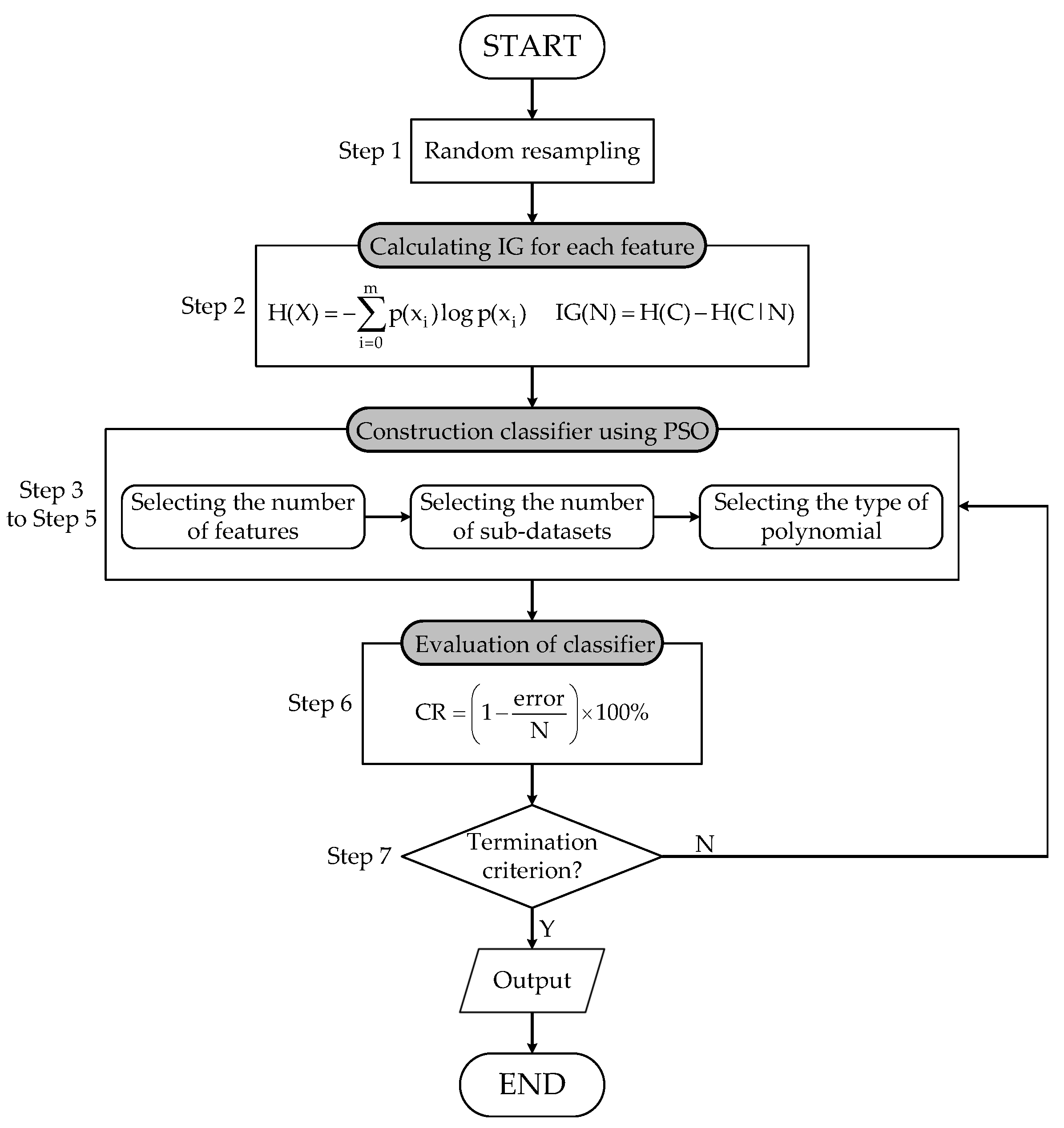
As shown in Figure 5, the OPNN-T is constructed using the parameter values optimized by the PSO algorithm. The optimization of the model includes the selection of the number of features, the number of sub-datasets, and the type of polynomial.

[Step 1] Perform random sampling on the input data, obtaining a subsample of size N through iterations.

[Step 2] Calculate the information gain for each feature according to Equation (11), and rank the features based on their information gain values. A higher information gain value indicates greater importance for the feature.

[Step 3] Determine the selected features. The first particle is responsible for selecting the number of features, processed via the RF algorithm. The randomly selected value is then rounded to the nearest integer. The decoded integer value represents the optimal dimensionality of the input variables within the feature data obtained through random sampling.

[Step 4] Determine the size of the selected sub-dataset. The second particle decides the size of the sub-dataset and adjusts it as necessary to enhance the model’s fitting capability. The randomly assigned value is also rounded to the nearest integer, and the selected sub-datasets are used for polynomial calculations.

[Step 5] Determine the type of polynomial. The third particle is tasked with determining the type of polynomial to be used, with the selected value similarly rounded to the nearest integer, corresponding to three different types of polynomials.

[Step 6] Evaluate the actual performance of each subset. The classification accuracy (CR) is used as the fitness value for the PSO objective function, and serves as the evaluation metric. The $CR$ can be expressed in the following form:

$$CR=\left(1-{\displaystyle \frac{error}{N}}\right)\times 100\%$$

(33)

where $error$ represents the total number of classification errors. N denotes the number of samples in the training set when the training accuracy (TR) is calculated. When computing the testing accuracy (TE), N represents the number of samples in the testing set. The training data are used to construct the model, whereas the test set is employed to validate the actual performance of the model.

[Step 7] Check for the termination condition: (1) the maximum number of iterations is reached, or (2) the global best fitness value shows no significant improvement over a predefined number of consecutive iterations. If the termination condition is not met, return to and repeat Steps 3 through 6. If the termination condition is satisfied, output the final results. These termination criteria ensure the stability and efficiency of the optimization process, making it suitable for the diverse datasets used in the experiments.

3.4. Computational Complexity Analysis

For the temporal feature enhancement module, the LSTM network is local in both time and space, which means that the input sequence length does not affect the complexity [31]. For each time step, the complexity for each weight is $O\left(1\right)$. Therefore, the complexity of the temporal feature enhancement module is $O\left(W\right)$, where W represents the number of weights.

For the PNNC, the complexity of the LSE in each polynomial neuron (PN) is $O\left({n_k}^3\right)$ [32], where $n_k$ denotes the dimension of the input values. Therefore, the complexity of the PNNC can be expressed as $O\left({n_k}^3\right)$.

For the self-optimization algorithm, the complexity of a single PSO iteration is determined by the fitness function. In the proposed model, the fitness function is derived from the PNNC. Therefore, the complexity of a single iteration is $O(m_s·{n_k}^3)$, where $m_s$ represents the swarm size. Considering that the algorithm requires T iterations to converge or reach the predefined maximum number of iterations, the complexity of the self-optimization algorithm is $O(T·m_s·{n_k}^3)$. In summary, the overall complexity of the proposed model can be expressed as

$$O(W+T·m_s·{n_k}^3)$$

(34)

4. Experiments and Results

4.1. Experimental Design

We compared the experimental results with those of the traditional models and other related models proposed by researchers. To evaluate the performance of the proposed model, we selected eight public machine learning datasets from the UCI benchmark for comparison. The models compared with the PNN and the self-optimized PNN (OPNN) are the latest standard machine learning classifiers available in scikit-learn [33]. The UCI datasets can be accessed at https://archive.ics.uci.edu/ml (accessed on 21 January 2025).

Furthermore, we chose 17 publicly available time series datasets to compare the differences between OPNN-T and some other models. Time series datasets can be accessed at https://timeseriesclassification.com/ (accessed on 21 January 2025). The datasets utilized in experiments span a wide range of characteristics, including number of features, number of classes, temporal complexity, and application domains. This diversity allows models to be tested under different conditions, ensuring that the performance of the models is evaluated comprehensively and potential limitations are identified across various scenarios.

In the PSO algorithm, different parameter values may yield varying results. The parameter values for our model were selected based on experiments and references from several existing models, as shown in

Table 1. Values of the parameters of the classifier.

Parameters	Values
Generation size	100
Swarm size	20
Vmin, Vmax	−1, 1
W	0.4
c1, c2	[1, 2]
No. of features	[2, no. of features]
No. of sub-datasets	[10, 30]
Types of polynomial	[1, 3]

. For the swarm size, we experimented with values of 10, 20, and 30. A smaller swarm size reduced computational cost but often resulted in suboptimal solutions, whereas a larger swarm size improved the quality of solutions at the expense of increased computation time. A swarm size of 20 provided a suitable balance between efficiency and solution quality. Similarly, for the inertia weight, values of 0.3, 0.4, and 0.5 were tested. A lower value encouraged exploitation by focusing on local search. However, a higher value promoted exploration at the cost of slower convergence. The inertia weight of 0.4 achieved consistent results in most cases and proved effective in balancing exploration and exploitation.

All the experiments used the classification rate as the evaluation metric, referring to Equation (33) for the calculation of the classification rate.

4.2. Experiments with Machine Learning Datasets

To validate the performance of the OPNN, we conducted experiments on eight different machine learning datasets obtained from the UCI database. The datasets were divided into a 60:40 ratio, with 60% of the data allocated for the training set and 40% for the testing set.

Table 2. Characteristics of the datasets.

Dataset	Number of Samples	Number of Features	Number of Classes
Fertility	100	10	2
Forest fires	244	13	2
Ionosphere	351	34	2
Seeds	210	7	3
Vehicle	846	18	4
WDBC	569	30	2
Wine	178	13	3
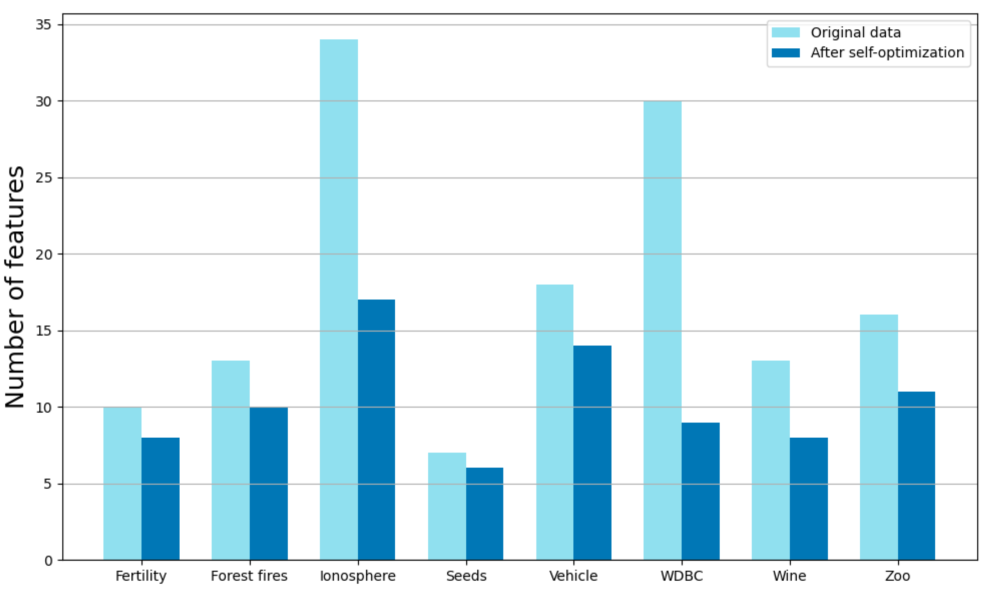
Zoo	101	16	7

summarizes the relevant characteristics of these eight datasets, including the number of samples, the number of features, and the number of classes. The optimization includes selected features, the size of the chosen sub-dataset, and the type of polynomial.

Table 3. Parameter results of the classifier after optimization.

Dataset	No. of Selected Features	No. of Sub-Dataset Selections	Type of the Polynomial
Fertility	8	9	3
Forest fires	10	2	3
Ionosphere	17	8	1
Seeds	6	17	3
Vehicle	14	10	2
WDBC	9	14	2
Wine	8	6	2
Zoo	11	13	3

presents the parameter results of the classifier after optimization. Figure 6 compares the number of original features with the number of features selected after optimization.

Multiple randomly sampled sub-datasets were fed into the polynomial neurons of the classifier, enabling the model to achieve good generalization capabilities.

Table 4. Classification rate of the OPNN.

Data	TR	TE
Fertility	90.00	92.50
Forest fires	98.63	98.98
Ionosphere	98.58	91.43
Seeds	97.62	98.81
Vehicle	87.57	80.53
WDBC	97.38	96.77
Wine	99.12	98.44
Zoo	98.55	100.00

displays the classification accuracy for both training and testing data. As described in Section 3, the fitness of the objective function refers to the classification rate of the training data, with TR and TE representing the classification rate of the training and testing sets, respectively.

Table 5. Comparison of the classification rates of the classifiers.

Data	KNN [33]	SVM [33]	Bayes [33]	Logistic [33]	Decision Tree [33]	RF [33]	AdaBoost [33]	PNN	OPNN
Fertility	87.50	90.00	92.50	90.00	80.00	92.50	85.00	90.00	92.50
Forest fires	90.28	98.98	92.86	97.96	97.96	97.96	97.96	95.92	98.98
Ionosphere	82.86	90.71	87.86	89.29	87.14	92.86	91.43	90.71	91.43
Seeds	85.71	91.67	90.48	92.86	90.48	91.67	86.90	97.62	98.81
Vehicle	61.36	78.76	43.36	80.24	69.62	71.68	55.75	77.58	80.53
WDBC	97.13	97.13	96.77	97.13	92.47	96.77	95.70	95.70	96.77
Wine	64.06	93.75	96.88	96.88	87.50	98.44	84.38	92.19	98.44
Zoo	92.31	97.44	97.44	97.44	97.44	97.44	79.49	97.44	100.00

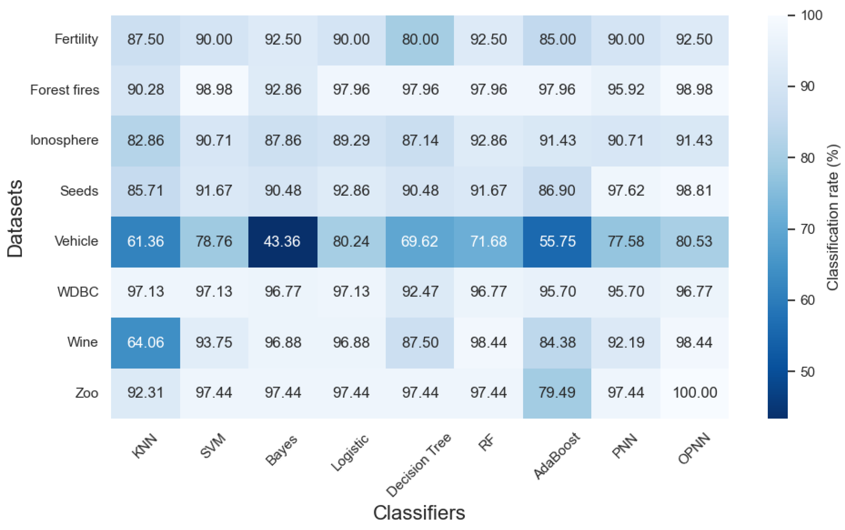
The best results are shown in bold.

and Figure 7 compare the classification rates of the proposed classifiers with those of classifiers from the literature and the traditional classification algorithms.

The experimental results in Table 5 demonstrate that OPNN consistently outperforms or matches other classification algorithms across a range of datasets. Specifically, OPNN achieved the highest classification rate in five out of the eight datasets, including Fertility, Forest Fires, Seeds, Vehicle, and Zoo. On the remaining three datasets, OPNN either matched the best-performing algorithm, as seen in the Forest Fires and Wine datasets or performed slightly below the top methods, as observed in WDBC. Notably, on the Seeds dataset, the OPNN achieves a classification rate of 98.81%, surpassing the strong performance of the PNN of 97.62%, which highlights the effectiveness of the optimization process in enhancing classification accuracy. In datasets with well-separated and clearly distinguishable features, such as Zoo and Seeds, OPNN demonstrates notable advantages, outperforming even ensemble-based algorithms such as random forest and AdaBoost. However, in datasets with overlapping class boundaries or less distinct feature patterns, such as WDBC and Ionosphere, OPNN’s performance remains competitive but does not show a substantial improvement over the best baseline methods.

Additionally, OPNN shows a significant improvement over PNN in datasets such Vehicle and Forest Fires, further emphasizing the impact of the optimization process. These findings highlight OPNN’s robustness and adaptability across diverse datasets, particularly for scenarios involving complex or nonlinear data patterns. However, it is also evident that in datasets where multiple algorithms already achieve near-perfect accuracy, such as WDBC and Zoo, the relative improvement offered by OPNN may appear less pronounced due to the inherently high baseline performance. Overall, the results underline OPNN’s capacity to maintain consistent, and high levels of classification accuracy while demonstrating adaptability across a broad range of data conditions.

4.3. Experiments with Time Series Datasets

To further validate the capabilities of the proposed model, we conducted experiments on 17 different publicly available time series datasets. Figure 8 illustrates the time series features corresponding to different labels (0 and 1) in the earthquake dataset.

Table 6. Characteristics of the time series datasets.

Dataset	Number of Samples	Number of Features	Number of Classes
BeetleFly	40	512	2
DistalPhalanxOAG	539	80	3
DistalPhalanxOC	876	80	2
DistalPhalanxTW	539	80	6
Earthquakes	461	512	2
ECG200	200	96	2
ECG5000	5000	140	5
Ham	214	431	2
Herring	128	512	2
ItalyPowerDemand	1096	24	2
MiddlePhalanxOAG	554	80	3
MiddlePhalanxOC	891	80	2
MiddlePhalanxTW	553	80	6
OliveOil	60	570	4
ProximalPhalanxOAG	605	80	3
ProximalPhalanxOC	891	80	2
ProximalPhalanxTW	605	80	6

summarizes the relevant characteristics of these 17 datasets, including the number of samples, the number of features, and the number of classes.

Table 7. Classification rate of OPNN-T.

Data	TR	TE
BeetleFly	100.00	95.00
DistalPhalanxOAG	88.00	77.70
DistalPhalanxOC	84.33	75.00
DistalPhalanxTW	83.00	73.38
Earthquakes	100.00	76.98
ECG200	100.00	95.00
ECG5000	98.20	94.16
Ham	99.08	80.95
Herring	85.94	75.00
ItalyPowerDemand	100.00	96.40
MiddlePhalanxOAG	80.50	66.88
MiddlePhalanxOC	83.50	76.63
MiddlePhalanxTW	79.70	61.04
OliveOil	100.00	93.33
ProximalPhalanxOAG	90.25	88.78
ProximalPhalanxOC	87.50	86.94
ProximalPhalanxTW	88.75	82.44

presents the classification accuracy for both the training and testing data, with TR and TE indicating the classification accuracy of the time series training and testing sets, respectively.

Table 8. Comparison of the time series classification rate with the proposed models.

Dataset	OPNN	OPNN-T (Linear Polynomial)	OPNN-T (Without Sub-Datasets)	OPNN-T
BeetleFly	85.00	90.00	80.00	95.00
DistalPOAG	71.22	74.82	67.63	77.70
DistalPOC	67.03	71.01	73.19	75.00
DistalPTW	60.43	70.50	58.27	73.38
Earthquakes	67.63	71.22	75.54	76.98
ECG200	93.00	92.00	90.00	95.00
ECG5000	92.42	94.16	93.87	94.16
Ham	66.67	79.04	76.19	80.95
Herring	68.75	71.88	64.06	75.00
ItalyPD	96.99	96.40	96.21	96.40
MiddlePOAG	60.39	64.29	61.04	66.88
MiddlePOC	64.95	61.17	74.91	76.63
MiddlePTW	56.49	61.04	56.49	61.04
OliveOil	80.00	90.00	93.33	93.33
ProximalPOAG	86.34	87.32	84.39	88.78
ProximalPOC	81.10	81.79	86.60	86.94
ProximalPTW	78.05	82.44	77.07	82.44

The best results are shown in bold.

compares the classification rates of different proposed models for time series classification, including OPNN-T, OPNN (without temporal feature enhancement), OPNN-T (with only linear polynomial types), and OPNN-T (without the sub-dataset method).

Table 9. Comparison of the time series classification rate with the classifiers.

Data	RF [33]	AdaBoost [33]	TBOPE [21]	RSFCF [22]	AFFNet [23]	OPNN	OPNN-T
BeetleFly	90.00	85.00	85.00	85.00	85.00	85.00	95.00
DistalPOAG	75.54	40.29	76.25	74.82	74.10	71.22	77.70
DistalPOC	78.26	76.45	73.91	78.26	76.40	67.03	75.00
DistalPTW	70.50	64.75	67.62	69.06	69.80	60.43	73.38
Earthquakes	74.82	75.54	74.82	74.82	74.80	67.63	76.98
ECG200	81.00	85.00	88.00	86.00	92.00	93.00	95.00
ECG5000	93.53	87.76	94.37	94.53	94.10	92.42	94.16
Ham	72.38	66.67	58.09	76.19	82.90	66.67	80.95
Herring	57.81	70.31	64.06	67.19	67.20	68.75	75.00
ItalyPD	95.63	95.24	94.07	96.02	97.50	96.99	96.40
MiddlePOAG	61.04	59.09	58.44	62.99	54.50	60.39	66.88
MiddlePOC	82.13	73.54	77.66	83.16	81.80	64.95	76.63
MiddlePTW	57.14	52.60	56.49	58.44	50.00	56.49	61.04
OliveOil	90.00	73.33	86.66	83.33	76.70	80.00	93.33
ProximalPOAG	86.83	80.49	84.19	82.93	84.40	86.34	88.78
ProximalPOC	86.25	83.16	83.41	87.63	91.80	81.10	86.94
ProximalPTW	80.49	73.66	78.53	80.49	80.00	78.05	82.44

The best results are shown in bold.

compares the classification results of the proposed classifier with those of the classifiers referenced in the literature.

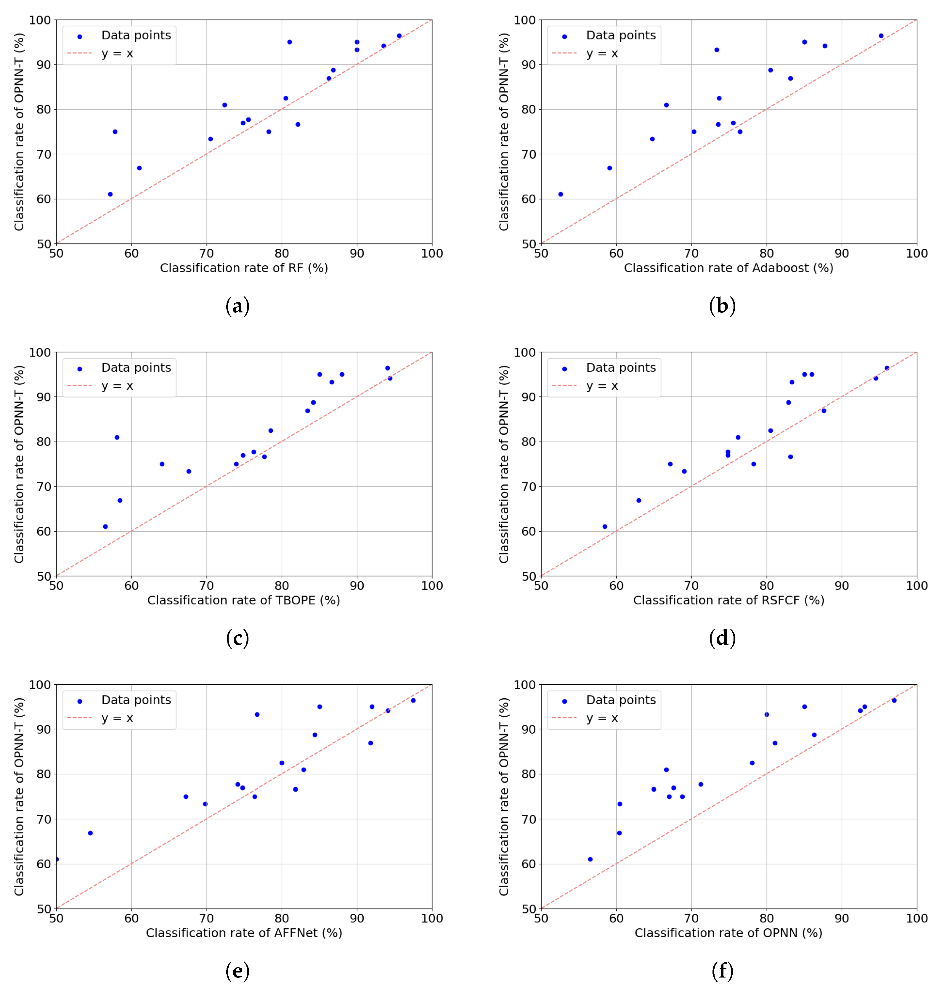
Figure 9 displays a comparison of accuracy results between OPNN-T and other classifiers, including RF, AdaBoost, TBOPE, RSFCF, AFFNet, and OPNN.

Table 10. Results of the Wilcoxon signed-rank test comparing OPNN-T with the other models.

Comparison Model	p Value
RF	0.007904
AdaBoost	0.000076
TBOPE	0.000076
RSFCF	0.012863
AFFNet	0.034790
OPNN	0.000031

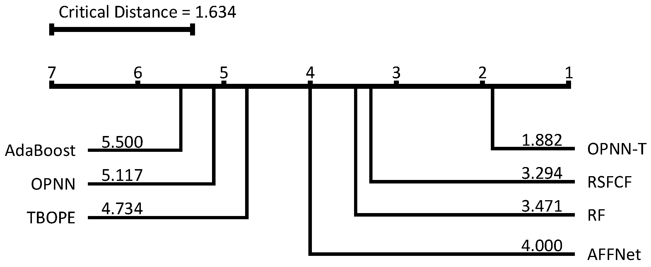
presents the results of the Wilcoxon signed-rank test conducted to compare the OPNN-T with six other models. Figure 10 provides the average ranking and critical difference diagram for the seven classifiers across the 17 datasets.

The experimental results indicate that the proposed model not only significantly outperforms traditional classification algorithms in terms of the classification rate, but also has advantages over recently developed time series classification models. Specifically, OPNN-T achieved the highest classification rate in 12 out of the 17 time series datasets, while maintaining competitive performance in the remaining five datasets. To further validate the statistical significance of OPNN-T’s performance improvements, we conducted a Wilcoxon signed-rank test to compare its classification rates with those of the baseline models across the 17 datasets. The results of the test revealed that the p values for all comparisons with the baseline models were consistently less than 0.05, indicating that the observed performance improvements of OPNN-T are statistically significant. This demonstrates that OPNN-T not only achieves superior performance in terms of average ranking but also provides consistent and reliable advantages over a variety of classification models, including both the traditional classifiers and state-of-the-art time series classification models.

The excellent performance of OPNN-T can be attributed to its architectural design, which combines self-optimizing polynomial neural networks with a temporal feature enhancement module. As shown in the results of Table 8, temporal feature enhancement and the self-optimization approach have varying impacts on the model’s performance. Temporal feature enhancement enables the model to capture more critical time series features. The diverse types of polynomials and the sub-dataset generation method further improve the classification rate of the model in different scenarios. Specifically, the best results for 4 of the 17 datasets were achieved via linear polynomials, which means that the performance on the remaining 13 datasets benefited from higher-order polynomials. Additionally, the sub-dataset generation method often outperforms the performance observed on the full dataset, effectively reducing the model’s overreliance on the training data.

The design of OPNN-T provides a distinctive methodological perspective compared to existing models, addressing certain challenges they face under specific conditions. For instance, TBOPE uses the SAX symbolization method, which predominantly captures the average and trend features of time series data. While effective in certain scenarios, this method may overlook other critical feature information, limiting its ability to fully represent the complexity of the data. RSFCF enhances computational efficiency by randomly selecting shapelets, and restricts their search range, effectively reducing computational overhead. However, this strategy can result in the loss of shapelet location information and insufficient discriminative features, which may ultimately impact the classification rate.

OPNN-T generally demonstrates superior adaptability in time series classification tasks compared to OPNN; its performance on the ItalyPowerDemand dataset is slightly suboptimal. This may be attributed to several factors. First, the dataset is characterized by a limited number of features and lacks the pronounced long-term temporal dependencies observed in other datasets, such as those with periodic or seasonal patterns. As the OPNN-T is specifically designed to capture complex temporal dynamics, its advantage becomes less pronounced when such characteristics are absent. Second, the relatively low variability within the dataset may reduce the model’s ability to leverage its advanced feature extraction mechanisms, leading to a classification performance closer to that of the simpler models.

5. Conclusions

This study presents a novel self-optimizing polynomial neural network with temporal feature enhancement for time series classification, referred to as OPNN-T. The proposed model consists of a temporal feature enhancement module and PNNC, which uses three types of polynomial functions and employs self-optimization. Experimental results on 17 publicly available time series machine learning datasets indicate that the classification rate of the proposed model surpasses that of general models and several time series classification models reported in related literature.

OPNN-T offers significant potential for integration into a variety of practical applications where accurate time series classification is essential. For instance, in the domain of financial analysis, the model can be applied to detect anomalies in trading patterns by leveraging its ability to extract and enhance temporal dependencies from noisy and volatile time series data. In healthcare, it could support diagnostic systems by analyzing biomedical signals, such as ECG or electroencephalograms (EEGs), to identify irregularities indicative of diseases. Furthermore, in industrial settings it might be utilized in predictive maintenance systems to detect early warning signs of equipment failures, thereby reducing downtime and preventing costly repairs. These applications underscore the versatility of the model, as it is capable of adapting to diverse data characteristics while maintaining high predictive performances.

Despite the model’s promising applicability, its performance on certain datasets, especially those characterized by high noise levels or complex temporal dynamics, is not yet optimal, suggesting potential avenues for future refinements. To address these limitations, and ensure the broader applicability of the model, we plan to further optimize its core architecture. For example, replacing the current polynomial neurons with fuzzy polynomial neurons may enhance the model’s capability for nonlinear feature extraction and improve its robustness in handling noisy or irregular time series data. Furthermore, to facilitate deployment in real-world systems, future work will also focus on improving computational efficiency and scalability. By addressing these aspects, the proposed model holds promise as a more versatile and effective tool for diverse time series classification tasks, bridging the gap between theoretical innovation and practical implementation.