A Sequence Prediction Algorithm Integrating Knowledge Graph Embedding and Dynamic Evolution Process

Abstract

Sequence prediction is widely applied and has significant theoretical and practical application value in fields such as meteorology and medicine. Traditional models, such as LSTM(Long Short-Term Memory) and GRU(Gated Recurrent Unit), may perform better than this model when dealing with short-term dependencies, but their performance may decline on long sequences and complex data, especially in cases where sequence fluctuations are significant. However, the Transformer requires a large amount of computing resources (parallel computing) when dealing with long sequences. Aiming to solve the problems existing in sequence prediction models, such as insufficient modeling ability of long sequence dependencies, insufficient interpretability, and low efficiency of multi-element heterogeneous information fusion, this study embeds sequential data into the knowledge graph, enabling the model to associate context information when processing complex data and providing more reasonable decision support for the prediction results. Given the historical sequence and the predicted future sequence, three groups of sequence lengths were set in the experiment. And MAE (Mean Absolute Error)and MSE (Mean Square Error) are used as indicators for sequence prediction. In sequence prediction, dynamic evolution is conducive to enhancing the ability of the prediction model to capture the changing patterns of the current time series data and significantly improving the reliability of the prediction results. Experiments were conducted using five datasets from different application fields to verify the effectiveness of the prediction model. The experimental results show that based on the randomization of the prediction time step, the prediction model proposed in this study significantly improves the expression performance of stationary sequences. It has addressed the shortcomings of these traditional methods, such as maintaining good performance in the case of short sequences with large fluctuations.

1. Introduction

Sequence prediction refers to using data from a certain period in the past to predict information for a certain period in the future. It includes continuous prediction (numerical prediction and range estimation) and discrete prediction (event prediction). It has extremely high commercial value. Its main task is to predict the future value of a certain indicator based on its historical data. Sequence prediction has a wide range of applications, such as meteorological prediction [1], 2.5-µm Particulate Matter prediction [2], traffic congestion prediction [3], and so forth, providing technical support for many information application scenarios in society.

The long short-term memory network (LSTM) and the gated recurrent unit (GRU) models have enhanced the ability of sequence prediction models to handle long sequence data and capture long-term dependencies from a new technical perspective. For example, Hidasi et al. adopted the idea of the GRU model in the recommendation system [4], that is, using the GRU to model the sequence and capture the relationship of behavioral changes in the long sequence.

The application of the attention mechanism [5] has led to significant technological advancements in information processing methods, particularly in terms of long-distance dependent capture. Wen et al. proposed using a double-layer LSTM as the encoder and the decoder [6]. An attention mechanism was introduced between the encoder and the decoder, thereby enabling the model to capture the key information in the input sequence more accurately. The Transformer proposes the self-attention mechanism and parallel processing capability [7] to address the problem of long-distance dependencies and is now widely used in sequence prediction tasks. The SASRec (Self-Attentive Sequential Recommendation) model adopts the Transformer encoder as its backbone for sequence prediction [8]. This method alleviates the overly dependence of the sequence model on the current input variable by obtaining the global information of the sequence.

The sequence prediction task is diverse, which is mainly reflected in the prediction of multiple related variables. Wang et al. proposed that sequence data should account for both target features and auxiliary information, which exhibit extremely complex spatial dependencies. To address these issues, Wang et al. proposed the AI-DTN (Digital Twin Network) model [9]. This model designed a GRU (AI-GRU) acting on auxiliary information. Three different gating units were added to the AI-GRU for coordinating the calculation of target features and auxiliary information. The AI-DTN model conducted autonomous reinforcement learning on the influence of different variables on the results by effectively integrating sequence information, target features, and auxiliary information.

The GNN architecture has been widely applied in the in-depth research of graph data structures, such as graph convolutional network [10] (GCN) and graph attention network [11] (GAT). GCN has the same function as the basic deep learning model CNN and is used for feature extraction. Graph data, when processed by a GCN, can effectively capture the characteristics of nodes and their neighbors, thus enhancing the model’s understanding of the graph structure. In a GCN, the weight of message passing depends only on the degree of nodes. In contrast, GAT adopts an attention mechanism to iteratively update the weights of message passing in the form of attention scores learned with the model parameters. GAT can effectively and dynamically aggregate information from neighboring nodes. We propose another idea for the research on graph sequence data augmentation. By estimating the emission probability, nodes within a sequence can be connected to nodes outside the sequence, thereby generating a new sample sequence and achieving graph sequence data augmentation [12].

Knowledge graphs are also a type of graphs. They establish different semantic connections among sample data in the form of triples (head entity, relationship, and tail entity). They can effectively capture complex data and ultimately extract the features of knowledge interaction. Knowledge graphs are widely applied in various application scenarios, such as question-answering systems [13], recommendation systems [14], and so forth. Significant progress has also been made in the exploration of methods integrating sequence prediction with knowledge graphs. This method uses the triplet information extracted from the knowledge graph and hence enables the model to better capture the user’s interest characteristics and their evolution, thereby achieving more precise personalized recommendations in sequence prediction.

Sequence prediction, as the core task of time series data analysis, has significant application value in scenarios such as meteorology, medical care, and recommendation systems. In recent years, dynamic evolution modeling has become a key direction for improving the performance of sequence prediction, with the core lying in capturing the dynamic change patterns of the system over time. Most existing studies are based on deep learning frameworks. For instance, DIEN tracks user behavior changes through an interest evolution layer, DNE and JODIE, respectively, depict structural evolution from the perspectives of dynamic network embedding and node trajectory modeling, while DySAT captures evolution patterns in dynamic graph structures with the help of graph attention networks and temporal snapshots. Although these methods perform well in specific tasks, existing sequence prediction models still have obvious limitations: First, their modeling ability for complex sequences (high-dimensional, nonlinear, and implicit patterns) is limited, and traditional models and some depth methods find it difficult to accurately capture their intrinsic patterns; Second, there is insufficient long-term dependence modeling. The model is easily dominated by short-term dependence, and the remote associated information gradually decays during the transmission process. Thirdly, the ability to cross-integrate multiple relationships is weak. The complex dependencies among multiple variables introduce noise and affect the stability of the model. In addition, semantic enhancement methods such as graph structures, while introducing rich relational information, also bring significant computational burdens, restricting the scalability of actual systems. To address the above challenges, this paper proposes a dynamic evolution sequence prediction method integrating knowledge graph embeddings. This method employs sequence data into a dynamic knowledge graph to explicitly model the temporal correlations and semantic relationships between entities, thereby enhancing the ability to capture long-term dependencies and the interpretability of the model. Meanwhile, an efficient structural evolution mechanism should be designed to control the computational complexity while introducing external knowledge, thereby enhancing the prediction accuracy and robustness for multivariate complex sequences.

Sequence prediction, as the core task of time series data analysis, is gradually shifting from relying solely on historical value matching to exploring the complex entity relationships and evolution patterns behind the data. Against this backdrop, knowledge graph embeddings are introduced into sequence prediction, providing the model with rich semantic context. By mapping entities in the sequence (such as users, products, and symptoms) to a low-dimensional vector space, knowledge graph embeddings can explicitly encode multi-hop associations (such as class, subordination, and causality) among entities, enabling the model not only to learn temporal patterns but also to perform relational reasoning, thereby enhancing the interpretability of predictions, especially when the data is sparse or there are cold start problems.

However, static knowledge graphs cannot fully reflect the dynamics of relationships in the real world. Therefore, dynamic evolution modeling becomes a key supplement. This type of method aims to capture the structural changes in the system over time, for example, by modeling the relationships of addition, disappearance or intensity change through temporal knowledge graphs or dynamic graph neural networks. This, when combined with sequence modeling, enables the model to synchronously track the evolution of entity states and the changes in their relationship networks, thereby more accurately capturing long-term dependencies. In this process, the attention mechanism plays a core role. It can adaptively weigh the importance of different historical time steps and different associations between entities. For instance, when predicting the next event, the model can focus on recent key events and their related entities, effectively filtering out noise.

At present, hybrid architectures that integrate these ideas have become mainstream and can mainly be classified into the following categories for comparative analysis:

GCN/ GNN-RNN hybrid model: This type of model typically uses GNN to encode the graph structure information at the current moment and then inputs the output to RNN (such as LSTM/GRU) to capture temporal dependencies. Its advantage lies in its clear structure, and RNN itself is a powerful sequence model. However, its limitations lie in the inherent sequential processing method and vanishing gradients of RNN, which make it difficult to effectively capture very long-term dependencies and result in relatively low computational efficiency.

Transformer–GNN hybrid model: This type of model utilizes the self-attention mechanism of Transformer to replace RNN for modeling temporal dependencies. Self-attention can perform parallel computing and directly capture global dependencies between any distant time steps, significantly outperforming RNNS on long sequences. GNN is responsible for extracting structural information at each time step. The combination of the two (such as GraphTransformer) is currently a cutting-edge direction, but its challenge lies in the fact that the computational complexity increases exponentially with the sequence length, and it requires meticulous design to effectively integrate the graph structure information into the attention calculation.

Specialized architectures based on dynamic evolution: In addition to the above-mentioned general hybrid models, architectures specifically designed for dynamic graphs (such as DyRep and TGN) have emerged. They treat sequential events (such as interactions) as continuous flows and update the embeddings of affected nodes each time an event occurs. This type of model seamlessly integrates sequence prediction with graph evolution, making it particularly suitable for scenarios with frequent updates. However, it places higher demands on the model’s continuous-time modeling capability and computational efficiency.

In conclusion, dynamic sequence prediction based on knowledge graph embedding represents an important development direction in this field. Through comparison, it can be known that the Transformer–GNN hybrid model has the greatest potential in capturing long-range and global dependencies. However, how to balance its expressive power and computational cost, and more precisely integrate temporal and structural attention, remains a key gap and challenge in current research.

2. Sequence Prediction, Knowledge Graph Embedding, and Dynamic Evolution Process

2.1. Problem Definition of the Sequence Prediction Model

The sequence prediction method achieves the purpose of predicting future-related trends in the scene by analyzing and modeling historical sequences. Suppose a historical sequence sample ${\mathrm{X}}_{1~\mathrm{L}}=\{{\mathrm{x}}_1,{\mathrm{x}}_2,...,{\mathrm{x}}_{\mathrm{L}-1},{\mathrm{x}}_{\mathrm{L}}\}$, where $(\mathrm{x}\in {\mathrm{X}}_{1~\mathrm{L}})$ is a single sequence sample. The expression of the sequence prediction model is shown in Equation (1), where ${\widehat{\mathrm{y}}}_{1+\mathrm{L}}$ represents the predicted value at the next time point, F represents the sequence prediction model, and L represents the length of the historical sequence.

$${\widehat{y}}_{1+L}=F\left(X_{1~L}\right)$$

(1)

Sequence prediction models are applied in various application scenarios to predict the possible outcomes of a certain event in the future. The practical application examples of Equation (1) are expounded by listing several typical application scenarios.

(1)

Sequence prediction based on classification: Common scenarios include the click-through rate (CTR) prediction task [15]. CTR is one of the important indicators for measuring the benefits of a product. In the sequence prediction task, ${\widehat{\mathrm{y}}}_{1+\mathrm{L}}$ has only two values: 0 and 1.0, respectively, representing that the user dislikes or likes the product.

(2)

Sequence prediction based on regression and multi-step time: Common regression scenarios include temperature, humidity, and other indicators. The values of these indicators exist within a certain range [16]. A typical multi-step application scenario of time-series prediction is weather forecasting. This scenario not only takes the next time prediction point as a parameter but also simultaneously inputs multiple future time prediction points into the model for prediction purposes. If the set parameters are as ${\widehat{\mathrm{Y}}}_{\mathrm{L}~\mathrm{T}}=\{{\widehat{\mathrm{y}}}_{\mathrm{L}},{\widehat{\mathrm{y}}}_{\mathrm{L}+1},...,{\widehat{\mathrm{y}}}_{\mathrm{L}+\mathrm{T}}\}$, then a single future point in time is denoted as $\widehat{\mathrm{y}}(\widehat{\mathrm{y}}\in {\widehat{\mathrm{Y}}}_{\mathrm{L}~\mathrm{T}})$. Here, T represents the length of the future time point. The expression of this type of sequence prediction model is as:

$${\widehat{Y}}_{L~T}=F(X_{1~L}).$$

(2)

2.2. Embedding of Knowledge Graphs

The knowledge graph is one of the key technologies in artificial intelligence, first proposed by Google in 2012. It is a structured semantic knowledge base that represents semantic relationships between entities in the form of triples (head entity, relation, and tail entity) [17]. Compared with other graph computing approaches, the symmetrical edges of a knowledge graph are of different types. In 2013, the TransE model was proposed as the most fundamental translation distance model. Suppose the head entity vector is Head, the relation vector is Relation, and the tail entity vector is Tail. The spatial position of the TransE model is shown in Figure 1.

$$h+r=t$$

(3)

The parameter relationship of the TransE model follows Equation (3), which indicates that the tail entity can be obtained by translating the head entity vector with the relation vector. The loss function of TransE is defined as:

$${\mathrm{l}\mathrm{o}\mathrm{s}\mathrm{s}}_E=\mathrm{m}\mathrm{a}\mathrm{x}(0,{‖h+r-t‖}_2-{‖h^{\prime }+r-t^{\prime }‖}_2+m)$$

(4)

In the aforementioned equation, ${\mathrm{h}}^{\prime }$ and ${\mathrm{t}}^{\prime }$ are, respectively, the head entity vector and the tail entity vector obtained by negative sampling. ${‖\mathrm{h}+\mathrm{r}-\mathrm{t}‖}_2$ is the vector modulus of positive sampling. ${‖{\mathrm{h}}^{\prime }+\mathrm{r}-{\mathrm{t}}^{\prime }‖}_2$ is the vector modulus of negative sampling. The operation of negative sampling is adopted to avoid the problem of deliberately reducing the vector moduli of $\mathrm{h}$, $\mathrm{r},$ and $\mathrm{t}$ during the training process of the model. The max function is used to take the maximum value so as to prevent the loss value from being negative. $\mathrm{m}$ is a hyperparameter used to prevent phenomena such as overfitting in the model.

The training performance of the TransE model is poor in handling one-to-many, many-to-one, many-to-many, and reflexive relationships. To address these issues, TransH proposed a new model in 2014 [18]. The spatial position of the TransE model is shown in Figure 2. The core idea is to define a hyperplane ${\mathrm{w}}_{\mathrm{r}}$ for each relation, with ${\mathrm{h}}_{\perp }$ and ${\mathrm{t}}_{\perp }$ as the projections of $\mathrm{h}$ and $\mathrm{t}$ on ${\mathrm{w}}_{\mathrm{r}}$. The loss function of TransH can be defined as:

$$h_{\perp }=h-w_r^T\times h\times w_r$$

(5)

$$t_{\perp }=t-w_r^T\times t\times w_r$$

(6)

$${\mathrm{l}\mathrm{o}\mathrm{s}\mathrm{s}}_E=\mathrm{m}\mathrm{a}\mathrm{x}(0,{‖h_{\perp }+r-t_{\perp }‖}_2-{‖h_{\perp }^{\prime }+r-t_{\perp }^{\prime }‖}_2+m)$$

(7)

In Equations (5) and (6), the ${\mathrm{w}}_{\mathrm{r}}$ vector is the normal vector of the hyperplane ${\mathrm{w}}_{\mathrm{r}}$. The effects of each parameter in Equation (7) are consistent with those in Equation (4). The difference between the TransH and TransR models is that the TransH model maps entities to the hyperplane of relations whereas the TransR model maps entities to the vector space of relations [19]. The schematic diagrams of the two models are shown in Figure 3.

TransE is suitable for simple relationships, but its ability to model complex ones is limited. After investigation, it is found that RotatE and ConvE do perform well in the knowledge graph embedding task. Considering the complexity and reproduction difficulty of the current knowledge graph embedding models, TransR, which has low computational complexity and high interpretability, was chosen.

Suppose the dimension of the $\mathrm{r}$ vector is $\mathrm{d}$. Multiply the points $\mathrm{h}$ and $\mathrm{t}$ by a $\mathrm{k}\times \mathrm{d}$ matrix. The head entity hr and the tail entity tr mapped to the relation vector space can be obtained. The loss function of TransH is expressed as:

$$h_r=h\times M_r$$

(8)

$$t_r=t\times M_r$$

(9)

$${\mathrm{l}\mathrm{o}\mathrm{s}\mathrm{s}}_R=\mathrm{m}\mathrm{a}\mathrm{x}(0,{‖h_r+r-t_r‖}_2-{‖h_r^{\prime }+r-t_r^{\prime }‖}_2+m)$$

(10)

The entity is the corresponding feature vector, precisely the vector embedded through Embedding, allowing the model to deeply explore the potential features under that date. For instance, in the eyes of the model, July is seen as hot and humid, etc. How is the hidden state of GRU generated as a relation vector? It represents the hidden feature of the KG “relation” (triple r). Just a few specific numerical features seem like statistical methods rather than deep learning methods. Just a few specific numerical features need to be transformed by machine learning into a set of relational r feature vectors that can make the dimension of the embedding layer vector equal. Ensure that the vector addition of u + r = o is feasible, rather than having one vector with a large dimension and the other with a small dimension.

2.3. Dynamic Evolution Method

Dynamic evolution refers to the changes in a system over time and is widely used in sequence prediction tasks. The DIEN (Deep Interest Evolution Network) model of the recommendation system adopts the dynamic evolution method to track the changes in users’ interest behaviors [20]. The interest evolution layer of the DIEN model is shown in Figure 4. The dynamic evolution process of the DIEN model is expressed as:

$$\alpha =\mathrm{S}\mathrm{o}\mathrm{f}\mathrm{t}\mathrm{m}\mathrm{a}\mathrm{x}(x_t\times W_{\mathrm{a}\mathrm{t}\mathrm{t}}\times d)$$

(11)

$$\widetilde{u_t}=\alpha \times u_t$$

(12)

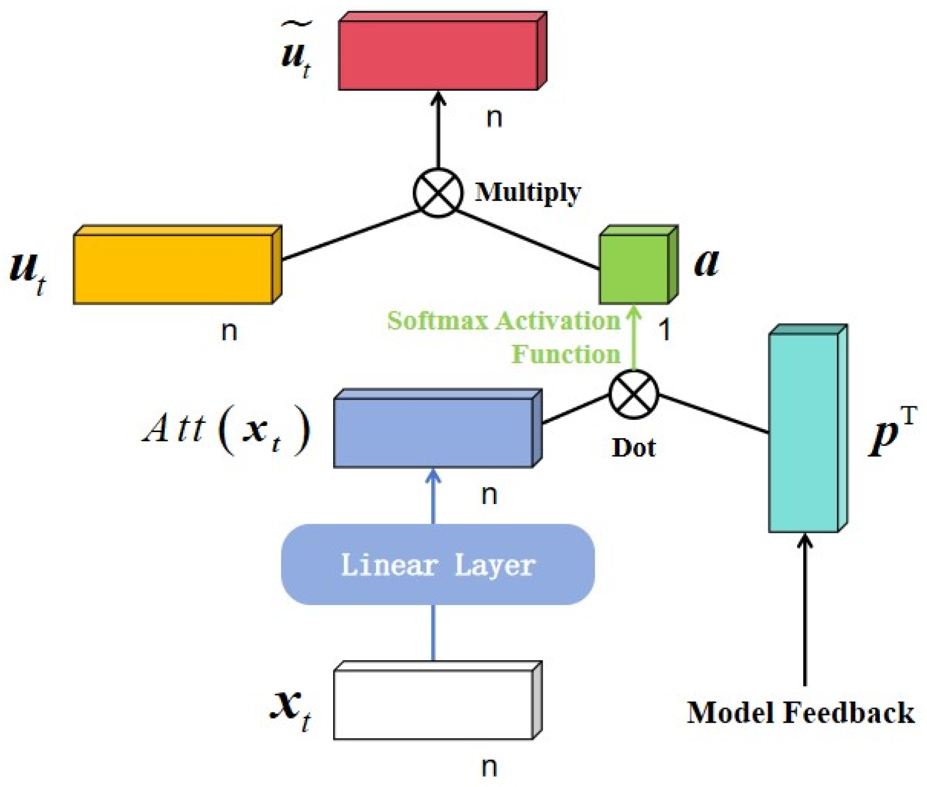
In the aforementioned equations, the attention score $\mathsf{\alpha }$ consists of the input ${\mathrm{x}}_{\mathrm{t}}$ at time $\mathrm{t}$, the target item $\mathrm{d}$ with information enhancement, and the parameter matrix ${\mathrm{W}}_{\mathrm{a}\mathrm{t}\mathrm{t}}$. Equation (11) uses the dot product to calculate the similarity between ${\mathrm{x}}_{\mathrm{t}}$ and $\mathrm{d}$. The higher the similarity between the two items, the greater the attention weight generated. The parameter matrix w is used for the linear transformation of x to improve the fit of the model. The attention score $\mathsf{\alpha }$ is multiplied by the update gate ${\mathrm{u}}_{\mathrm{t}}$ to adjust the importance of information, ensuring that the DIEN model focuses on highly relevant input when updating the state.

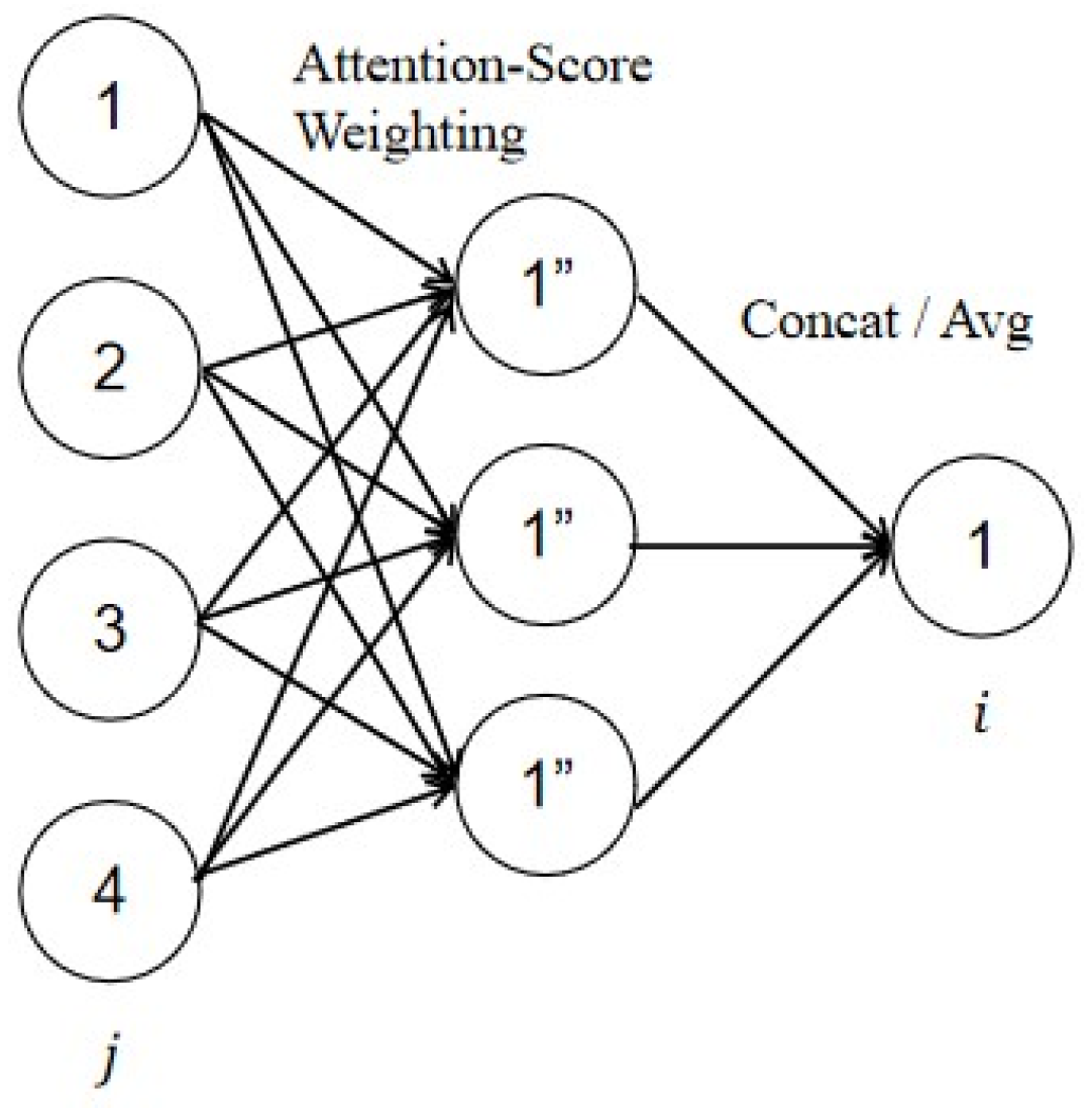
The DySAT (Deep neural representation learning of dynamic self-attention networks) model applies GAT for dynamic representation learning and divides the entire time period into multiple discrete snapshots using a time window to capture the dynamic evolution of the sequence [21]. The dynamic evolution of the DySAT model is mainly guided by GAT. The message-passing mechanism of the graph attention network of the DySAT model is shown in Figure 5.

The dynamic evolution mechanism of the DySAT model is expressed in Equations (13)–(15). Equation (13) is used to calculate the attention score ${\mathrm{e}}_{\mathrm{i}\mathrm{j}}$ from node $\mathrm{j}$ to node $\mathrm{i}$, where ${\mathrm{h}}_{\mathrm{i}}$ and ${\mathrm{h}}_{\mathrm{j}}$ are the input feature vectors of node $\mathrm{i}$ and node $\mathrm{j}$, respectively. It is assumed that their dimension is $\mathrm{F}$. $\mathrm{W}$ is the parameter matrix that the model needs to learn, with the dimension set as $\mathrm{F}\times {\mathrm{F}}^{\prime }$. The symbol “$\left|\right|$” represents the vector concatenation operation. $\mathsf{\beta }$ is also the attention vector that the model needs to learn, with the dimension of $2{\mathrm{F}}^{\prime }$. Finally, the result is obtained by activating the function LeakyReLU. Equation (14) is used to calculate the message-passing attention weight ${\mathrm{a}}_{\mathrm{i}\mathrm{j}}$ from node $\mathrm{j}$ to node $\mathrm{i}$, where ${\mathrm{N}}_{\mathrm{j}}$ represents the first-order neighbor set of node $\mathrm{i}$. Equation (15) is used to calculate the GAT result, that is, the feature vector ${\mathrm{h}}_{\mathrm{i}}^{\prime }$ of the new node $\mathrm{i}$, where $\mathsf{\sigma }$ is an activation function and $\mathrm{K}$ represents the number of information transmissions. The DySAT model can aggregate key information from neighboring nodes, capture the real-time evolution of graph data during training, and enhance the reasoning and predictive ability of the model for data evolution.

$$e_{ij}=L\mathrm{e}\mathrm{a}\mathrm{k}\mathrm{y}\mathrm{R}\mathrm{e}\mathrm{L}\mathrm{U}({\beta }^T[W\times h_i||W\times h_j])$$

(13)

$$a_{ij}={\displaystyle \frac{exp(e_{ij})}{{\sum }_{k\in N_i}exp(e_{ik})}}$$

(14)

$$h_i^{\prime }=\sigma ({\displaystyle \frac{1}{K}}{\sum }_{k=1}^K {\sum }_{j\in N_i}{a}_{ij}^k{x}^k{h}_j)$$

(15)

3. A Sequence Prediction Algorithm Integrating Knowledge Graph Embedding and Dynamic Evolution

To address issues such as insufficient modular ability, lack of interpretability, and low efficiency in fusing multi-heterogeneous information in most of the existing sequence prediction algorithms, this study proposed a sequence prediction algorithm integrating knowledge graph embedding and dynamic evolution, abbreviated as KD4SP.

3.1. Problem Definition of the KD4SP Algorithm

The problem addressed by the KD4SP algorithm is defined as follows: Given a historical sequence sample ${\mathrm{X}}_{1~\mathrm{L}}=\{{\mathrm{x}}_1,{\mathrm{x}}_2,...,{\mathrm{x}}_{\mathrm{L}-1},{\mathrm{X}}_{\mathrm{L}}\}$, where $\mathrm{x}(\mathrm{x}\in {\mathrm{X}}_{1~\mathrm{L}})$ is a single sequence sample and $\mathrm{L}$ is the fixed sequence window size. The characteristics of this historical sequence sample can be represented as ${\mathrm{E}}_{1~\mathrm{L}}=\{{\mathrm{e}}_1,{\mathrm{e}}_2,...,{\mathrm{e}}_{\mathrm{L}-1},{\mathrm{e}}_{\mathrm{L}}\}$. Based on the aforementioned conditions, the goal is to predict the future sequence ${\widehat{\mathrm{Y}}}_{\mathrm{L}+1:\mathrm{H}}=$ ${\widehat{Y}}_{\mathrm{L}+1\text{:}\mathrm{H}}=\left\{{\widehat{y}}_{L+1},{\widehat{y}}_{L+2},\dots ,{\widehat{y}}_H\right\}$, where $\mathrm{H}$ is the number of time steps for predicting the future.

3.2. KD4SP Algorithm Model

The KD4SP model is shown in Figure 6. It mainly includes four modules: the knowledge graph embedding layer, the dynamic evolution layer, the feature extraction layer, and the fully connected layer.

The KD4SP algorithm passes the sample data through the embedding layer and endows the samples with basic feature information. The features of the samples pass through the feature extraction layer, converting low-dimensional features into high-dimensional feature representations, extracting their hidden features. These features are then embedded together with the originally embedded sample data into the knowledge graph. The KD4SP algorithm inputs the hidden feature representation into the dynamic evolution layer to capture the changing trend of the sequence at this stage. Finally, the output result from the last layer of the dynamic evolution layer is then passed through a fully connected layer to obtain the predicted values. The knowledge graph embedding layer computes a scoring coefficient based on the knowledge graph embedding algorithm. The scoring coefficient mainly contributes to the loss function calculation of the model and plays a role in reinforcement learning.

Before embedding in the knowledge graph, the hidden features of the samples should be extracted to extract meaningful information and relationships. This ensures that the embedding better reflects the entities and the correlations among them, improving the performance and reasoning ability of the model. GRU is a typical sequence model. It dynamically adjusts the information flow of data through a gating mechanism, effectively capturing the long-term dependencies and key data [22]. Its structure is shown in Figure 7.

$$u_t=\mathrm{S}\mathrm{i}\mathrm{g}\mathrm{m}\mathrm{o}\mathrm{i}\mathrm{d}(W_u\times x_t+U_u\times h_{t-1}+b_u)$$

(16)

$$r_t=\mathrm{S}\mathrm{i}\mathrm{g}\mathrm{m}\mathrm{o}\mathrm{i}\mathrm{d}(W_r\times x_t+U_r\times h_{t-1}+b_r)$$

(17)

$${\tilde{h}}_t=tanh(W_h\times x_t+r_t\otimes U_u\times h_{t-1}+b_h)$$

(18)

$$h_t=(1-u_t)\otimes h_{t-1}+u_t\otimes {\tilde{h}}_t$$

(19)

The calculation of the GRU model is shown in Equations (16)–(19). ${\mathrm{x}}_{\mathrm{t}}$ represents the model input at time $\mathrm{t}$; $\mathrm{W}$, $\mathrm{U},$ and $\mathrm{b}$ are the parameters to be learned during the training process, and ${\mathrm{u}}_{\mathrm{t}}$ and ${\mathrm{r}}_{\mathrm{t}}$ represent the outputs of the update gate and reset gate at time $\mathrm{t}$, respectively. Both the update gate and the reset gate indicate how much hidden information from the previous moment is retained, and both are activated by the function Sigmoid. The closer the value range of ${\mathrm{u}}_{\mathrm{t}}$ and ${\mathrm{r}}_{\mathrm{t}}$ (0, 1) is to 1, the more information is retained. ${\tilde{\mathrm{h}}}_{\mathrm{t}}$ is the candidate hidden state, which is generated by combining the input ${\mathrm{x}}_{\mathrm{t}}$ at time $\mathrm{t}$ with the hidden state ${\mathrm{h}}_{\mathrm{t}-1}$ from the previous time step. Meanwhile, ${\tilde{\mathrm{h}}}_{\mathrm{t}}$ and the reset gate ${\mathrm{r}}_{\mathrm{t}}$ calculate the Hadamard product to control the transmission of information. The tanh activation function is used to compress the input value within the interval (−1, 1) to capture the important features at the current moment. The output result ${\mathrm{h}}_{\mathrm{t}}$ is jointly determined by ${\mathrm{h}}_{\mathrm{t}-1}$ and ${\tilde{\mathrm{h}}}_{\mathrm{t}}$, and the update gate ${\mathrm{u}}_{\mathrm{t}}$ plays the role of weighted combination. Essentially, it is the multiplication of matrices, ensuring that each vector is in the same semantic environment after a linear transformation, while the activation function is a nonlinear transformation.

Training sequence prediction algorithms only based on sample features is insufficient. Also, the model should learn the features of the samples to improve the validity of the data. The KD4SP algorithm adopts the embedding method for sample $\mathrm{x}$, and the vector is represented as its own features. Suppose the data after embedding is ${\mathrm{x}}^{\prime }$. As the knowledge graph embedding algorithm requires that the dimensions of entities and relations be the same, the entity features are the hidden information ${\mathrm{h}}_{\mathrm{t}}$ of the feature extraction layer. For the vector ${\mathrm{x}}_{\mathrm{A}}^{\prime }$ of entity A, the vector ${\mathrm{x}}_{\mathrm{B}}^{\prime }$ of entity B, and the feature ${\mathrm{h}}_{\mathrm{A}}$ of entity A, the triplet relationship is defined as:

$$x_A^{\prime }+h_A=x_B^{\prime }$$

(20)

Under the influence of its characteristics, Entity A evolves into Entity B. The KD4SP algorithm uses the TransR translation model, defining a different mapping matrix for each relation. This enables separate mapping for different relations, making the model more flexible and better able to capture complex relation features. Suppose the mapping matrix is ${\mathrm{M}}_{\mathrm{r}}$; the confidence score of the triplet relation can then be obtained as:

$$\mathrm{s}\mathrm{c}\mathrm{o}\mathrm{r}\mathrm{e}(x_A^{\prime }, h_A, x_B^{\prime })=‖{\mathrm{M}}_{\mathrm{r}}\times x_A^{\prime }+h_A+{\mathrm{M}}_{\mathrm{r}}\times x_B^{\prime }‖$$

(21)

The confidence score is also a parameter for measuring the loss function of the knowledge graph. The confidence value of the aforementioned triplet should be as small as possible. If the three vectors ${\mathrm{x}}_{\mathrm{A}}^{\prime }$, ${\mathrm{h}}_{\mathrm{A}}$, and ${\mathrm{x}}_{\mathrm{B}}^{\prime }$ decrease with their own moduli, $\mathrm{s}\mathrm{c}\mathrm{o}\mathrm{r}\mathrm{e}({\mathrm{x}}_{\mathrm{A}}^{\prime },{\mathrm{h}}_{\mathrm{A}},{\mathrm{x}}_{\mathrm{B}}^{\prime })$ also gets closer to 0. Therefore, a negative sampling method can be adopted to reduce their own moduli. During this process, a random number seed is generated between 0 and 1. When the value of seed is greater than 0.5, the function score randomly selects an entity from all entities and sets the first element member as the head pointer of the negative triplet. When the value of the seed is less than 0.5, a new sequence is generated. One entity is randomly selected from all entities, and the first element member is set as the head pointer of the positive triplet. This process is repeated in a loop until the number of positive triplets is half.

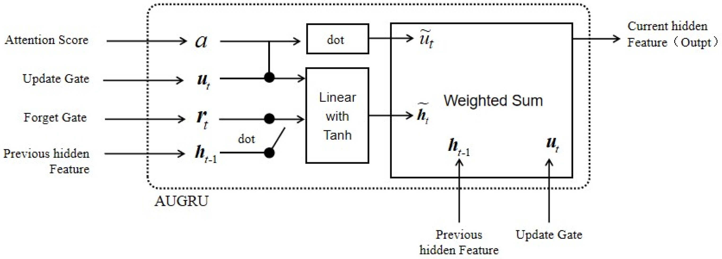
The current design models the dynamic features of samples and time steps by means of a learnable global weight vector p. Its main function is to weight the feature contributions of samples from different sequences at different time steps to capture the dynamic patterns of the data. For instance, at a certain historical moment t, if it makes a significant contribution and influences the subsequent process, then the weight value of this t in the weight vector p will be very high. The dynamic evolution layer of the KD4SP algorithm mainly comprises the AGRU (GRU with Attention) network [23]. AGRU adds an attention mechanism based on GRU. The AGRU network framework is shown in Figure 8.

The KD4SP model, by reusing the GRU state and combining it with the standard attention mechanism, although providing an efficient temporal reasoning framework, may be slightly less flexible and adaptable compared to the latest methods such as DySAT when dealing with highly dynamic and variable time series. DySAT may perform better than the KD4SP model when dealing with long-term dependencies and complex patterns, but the design of the KD4SP model places more emphasis on computational efficiency and real-time performance. The main difference between the two lies in the complexity of the dynamic attention mechanism and its adaptability to application scenarios.

Based on GRU, the calculation of the dynamic evolution process of each AGRU unit is depicted in Equations (22)–(24). ${\mathrm{x}}_{\mathrm{t}}$ represents the corresponding time output ${\mathrm{h}}_{\mathrm{t}}$ of the feature extraction layer. Equation (22) is a linear transformation of ${\mathrm{x}}_{\mathrm{t}}$ to improve the generalization ability of the model. ${\mathrm{W}}_{\mathrm{a}\mathrm{t}\mathrm{t}}$ and ${\mathrm{b}}_{\mathrm{a}\mathrm{t}\mathrm{t}}$ are the parameters that the model needs to learn; their dimensions are $\mathrm{n}\times \mathrm{n}$ and $\mathrm{n},$ respectively. Equation (23) calculates the attention score at the current moment, which is formed by the dot product of $\mathrm{A}\mathrm{t}\mathrm{t}\left({\mathrm{x}}_{\mathrm{t}}\right)$ and vector $\mathrm{p}$ and activated by the function Softmax. Vector $\mathrm{p}$ is the parameter that the model needs to learn, representing the feature weight coefficient; that is, the more important the feature, the higher the weight coefficient. The dimension of vector $\mathrm{p}$ is $\mathrm{n}$. The dot product of vector $\mathrm{A}\mathrm{t}\mathrm{t}\left({\mathrm{x}}_{\mathrm{t}}\right)$ and vector $\mathrm{p}$ is equivalent to the weighted summation effect, thus obtaining the total attention score $\mathrm{a}$ of all features. Then, the attention score is normalized by the activation of the function Softmax. Equation (24) resets the data of the update gate ${\mathrm{u}}_{\mathrm{t}}$, which is obtained by multiplying the attention score $\mathrm{a}$ by the update gate value ${\mathrm{u}}_{\mathrm{t}}$. The updated ${\mathrm{u}}_{\mathrm{t}}$ determines how much of the candidate hidden information at the current moment is retained. The update gate is related to the attention score, so the model can dynamically adjust the update process of the hidden state according to the different feature weight coefficients $\mathrm{p}$. As the weight coefficient $\mathrm{p}$ is obtained through continuous learning from historical data by the machine and through continuous attempts and adjustments, a dynamic evolution process can be achieved.

$$Att\left(x_t\right)=W_{\mathrm{a}\mathrm{t}\mathrm{t}}\times x_t+b_{\mathrm{a}\mathrm{t}\mathrm{t}}$$

(22)

$$\alpha =\mathrm{S}\mathrm{o}\mathrm{f}\mathrm{t}\mathrm{m}\mathrm{a}\mathrm{x}(p^{\mathrm{T}}\times Att(x_t\left)\right).$$

(23)

$${\tilde{u}}_t=\alpha \times u_t$$

(24)

The fully connected layer mainly comprises a combination of linear transformations and activation functions. The activation function is not set in the last layer of the fully connected layer. Considering the complexity of sequence data, the KD4SP algorithm adopts Dice (data-dependent activation function) as the activation function in the fully connected layers of the remaining levels [10] to address the problem of vanishing gradients caused by unsmooth data. The calculation method of Dice is depicted in Equations (25) and (26). Equation (25) represents the normalization processing of batch data. $\mathrm{E}\left(\mathrm{x}\right)$ represents the mean of the sample, $\mathrm{V}\mathrm{a}\mathrm{r}\left(\mathrm{x}\right)$ represents the variance of the sample, and $\mathsf{\xi }$ represents the noise factor. Equation (26) is used to calculate the Dice activation function. For $\mathrm{B}\mathrm{N}\left(\mathrm{x}\right)$, Sigmoid activation is adopted and expressed in the form of probability, assumed to be $\mathrm{p}(\mathrm{x}$). From the perspective of normalization, $\mathrm{p}\left(\mathrm{x}\right)$ represents the probability that the input value $\mathrm{x}$ is greater than the number corresponding to a Sigmoid threshold of 0.5. For example, if an array [−3, −2, …, 7] exists, then the number corresponding to a Sigmoid threshold of 0.5 is 2. The difference compared with ReLU-type activation functions, such as PReLU and LeakyReLU, is that the coefficient of the neuron is weakened only when the input value $\mathrm{x}$ is negative, as shown in Figure 9. The expected output value of the neuron is calculated using Equation (27). From a mathematical perspective, it can be understood as: finding the expected value E. The probability $\mathrm{p}\left(\mathrm{x}\right)$ is multiplied by $\mathrm{x}$ and $\mathsf{\alpha }\mathrm{x},$ respectively, where $\mathsf{\alpha }$ is a hyperparameter representing the coefficient of the neuron with weakened “negative characteristics.”

$$\mathrm{B}\mathrm{N}(x)={\displaystyle \frac{x-E\left(X\right)}{\mathrm{V}\mathrm{a}\mathrm{r}\left(x\right)+\xi }}$$

(25)

$$\mathrm{D}\mathrm{i}\mathrm{c}\mathrm{e}\left(x\right)=x\times \mathrm{S}\mathrm{i}\mathrm{g}\mathrm{m}\mathrm{o}\mathrm{i}\mathrm{d}\left(\mathrm{B}\mathrm{N}\right(x\left)\right)+\alpha \cdot x\cdot (1-\mathrm{S}\mathrm{i}\mathrm{g}\mathrm{m}\mathrm{o}\mathrm{i}\mathrm{d}(\mathrm{B}\mathrm{N}\left(x\right))$$

(26)

$$\mathrm{D}\mathrm{i}\mathrm{c}\mathrm{e}\left(x\right)=x·p\left(x\right)+\alpha \cdot x\cdot (1-p(x\left)\right)$$

(27)

The standardized data can be de-standardized before being input into the model if other requirements exist for the output of the model. Equation (28) is used to determine anti-standardization. This is the result of standardized negation. ${\mathrm{x}}_{\mathrm{r}\mathrm{e}\mathrm{a}\mathrm{l}}$ is the de-normalized value of ${\mathrm{x}}_{\mathrm{s}\mathrm{t}\mathrm{d}}$, $\mathsf{\sigma }$ is the standard value of the original data, and $\mathsf{\mu }$ is the mean value of the original data.

$$x_{\mathrm{r}\mathrm{e}\mathrm{a}\mathrm{l}}=\sigma ·x_{\mathrm{s}\mathrm{t}\mathrm{d}}+\mathsf{\mu }$$

(28)

The loss function of the model mainly has two parts: the auxiliary loss function and the predicted loss function. The auxiliary loss function is determined by the scoring coefficient of the knowledge graph embedding algorithm. The purpose of introducing the auxiliary loss function is to improve the training effect of the mode, thereby enhancing the learning ability of the model. The predicted loss function measures the gap between the predicted and true values. The model continuously learns and adjusts its own parameters based on this measurement value to achieve the best effect.

Suppose $\mathrm{loss}$ is the total loss function of the model. ${\mathrm{l}\mathrm{o}\mathrm{s}\mathrm{s}}_{\mathrm{a}\mathrm{u}\mathrm{x}}$ and ${\mathrm{l}\mathrm{o}\mathrm{s}\mathrm{s}}_{\mathrm{t}\mathrm{a}\mathrm{r}}$ represent the auxiliary and predicted loss functions of the model, respectively. $\mathsf{\gamma }$ is the weight proportion of the auxiliary loss function. The total loss function can be calculated using Equation (29). Deviations are inevitable during the training of the model. Therefore, an auxiliary loss function needs to be introduced to enhance the model’s learning of the knowledge graph embedding algorithm.

$$\mathrm{l}\mathrm{o}\mathrm{s}\mathrm{s}=\gamma ·{\mathrm{l}\mathrm{o}\mathrm{s}\mathrm{s}}_{\mathrm{a}\mathrm{u}\mathrm{x}}+{\mathrm{l}\mathrm{o}\mathrm{s}\mathrm{s}}_{\mathrm{t}\mathrm{a}\mathrm{r}}$$

(29)

The loss function of the knowledge graph embedding algorithm is influenced by the positive and negative sampling confidence scores [24]. ${\mathrm{x}}_{\mathrm{A}}^{\prime }$, ${\mathrm{h}}_{\mathrm{A}}$, and ${\mathrm{x}}_{\mathrm{B}}^{\prime }$ are the head entity, relation, and tail entity of positive sampling. Assuming that the negative sampling is ${\mathrm{x}}_{\mathrm{A}}^{\prime }$, ${\mathrm{h}}_{\mathrm{A}},$ and ${\mathrm{x}}_{\mathrm{B}}^{\prime }$, the auxiliary loss function can be calculated using Equations (30) and (31). The auxiliary loss value is calculated using Equation (30). $\mathrm{m}$ is a hyperparameter used to prevent phenomena such as overfitting of the model. Equation (31). ensures that the auxiliary loss value is non-negative.

$${\mathrm{l}\mathrm{o}\mathrm{s}\mathrm{s}}_{\mathrm{a}\mathrm{u}\mathrm{x}}^{\prime }=\mathrm{s}\mathrm{c}\mathrm{o}\mathrm{r}\mathrm{e}(x_A^{\prime },h_A,x_B^{\prime })-\mathrm{s}\mathrm{c}\mathrm{o}\mathrm{r}\mathrm{e}({\widehat{x}}_A^{\prime },{\widehat{h}}_A,{\widehat{x}}_B^{\prime })+m$$

(30)

$${\mathrm{l}\mathrm{o}\mathrm{s}\mathrm{s}}_{\mathrm{a}\mathrm{u}\mathrm{x}}=\left\{\begin{array}{c}{\mathrm{l}\mathrm{o}\mathrm{s}\mathrm{s}}_{\mathrm{a}\mathrm{u}\mathrm{x}}^{\prime } \mathrm{if} {\mathrm{l}\mathrm{o}\mathrm{s}\mathrm{s}}_{\mathrm{a}\mathrm{u}\mathrm{x}}^{\prime } \ge 0\\ 0 \mathrm{if} {\mathrm{l}\mathrm{o}\mathrm{s}\mathrm{s}}_{\mathrm{a}\mathrm{u}\mathrm{x}}^{\prime }<0\end{array}\right.$$

(31)

$$\mathrm{M}\mathrm{S}\mathrm{E}={\displaystyle \frac{1}{K}}\sum _{k=1}^K{(y_k-{\widehat{y}}_k)}^2$$

(32)

This study adopted the mean square error (MSE) as the prediction loss function. This was mainly because the MSE increased the penalty factor of the error. MSE is extremely sensitive to error, causing the model to place greater emphasis on data with large deviations from the true value during learning. The MSE can be calculated using Equation (28). $\mathrm{k}$ represents the sample size, and ${\mathrm{y}}_{\mathrm{k}}$ and ${\widehat{\mathrm{y}}}_{\mathrm{k}}$ represent the true and predicted values, respectively. The smaller the calculation result of Equation (32), the better the performance of the model fitting.

3.3. Construction of Knowledge Graph

Take the dataset Electricity as an example. The process of extracting entities and relationships from structured tables and storing them in the Neo4j graph database (Neo4j Community Edition 3.5.30 ) in the form of triples. The basic information of the dataset “Electricity” consists of date, electricity consumption, electricity generation, atomic energy, wind energy and other information.

The specific steps for constructing the knowledge graph of the dataset Electricity are as follows: First, clearly define the information form of the triples. In the sequence prediction task of this section, dates and feature values are used as nodes. Construct two types of triples: (current date, feature, current feature value) and (current feature value, influence, next day’s date). Secondly, import the neo4j graph database. Based on the above form, the logic for creating head and tail nodes and relationships is written using the py2neo library(python 3.8). Traverse each row of data in the table, create nodes for samples and their features, establish relationships between each sample node and its feature nodes, and establish an influence relationship between the previous feature node and the current sample node. A detailed description of the pseudo-code algorithm is provided in Appendix A. The KD4SP model maps the features at each time point to entities, with u + r = o as the training objective. That is to say, entity u evolves into o under the influence of relation r. Therefore, it is an end-to-end learning process.

This algorithm implements the following core logic: Construction of temporal relationship: The feature nodes of the time step on the last_feature_node_group are cached to ensure the correct establishment of the connection relationship on the time series. Graph structure pattern: Sample node → feature node: HAS_FEATURE relationship, feature node → next time step sample node: TEMPORAL_FLOW relationship. Data flow control: After processing all the features of a sample each time, clear the cache of the previous time step and prepare to receive new feature nodes. This design is suitable for constructing feature graphs with temporal dependencies and is particularly suitable for graph representation learning scenarios of time series data.

The KD4SP framework mainly consists of four modules: the knowledge graph embedding layer, the feature extraction layer, the dynamic evolution layer, and the fully connected layer. Among them, the knowledge graph embedding layer helps the model capture the context information of sequential data, thereby enhancing the model’s understanding and reasoning ability of the data. In addition, this paper also proposes a negative sampling method to solve the problem that the confidence score is also too low due to the excessively low modulus length. The feature extraction layer converts low-dimensional feature vectors into high-dimensional feature representations, helping the model better understand the correlation between feature data and sequence data. The dynamic evolution layer helps the model capture the changing patterns of the current time series data, thereby improving the accuracy and reliability of the prediction. The fully connected layer, through the combination of linear transformation and activation functions, enables the model to extract more complex features from the data and ultimately output the prediction results.

4. Experiments and Results

4.1. Experimental Dataset

The Electricity [25] dataset recorded the generation and consumption of electricity in the United States from 2019 to 2024 [26]. It included 10 groups of information such as atomic production capacity, wind production capacity, and petrochemical production capacity. A total of 46,012 sets of data were included. In the AvocadoPrice [27] dataset, the average price changes in avocados from 2015 to 2018 were recorded [28], including 13 sets of characteristic information such as total sales volume, total sales volume of 4046-type avocados, box sales volume, bag sales volume, and region. A total of 18,250 sets of data were included. The Traffic [29] dataset showed the traffic volume information of a certain place from 2012 to 2018 [30]. It included nine groups of information, mainly including whether it was a holiday, temperature, hourly rainfall, and hourly snowfall. A total of 48,205 sets of data were included. The Weather [31] dataset recorded the meteorological information of a certain place from January to March 2025 [17]. It comprised 22 sets of information, such as air pressure, temperature, relative humidity, precipitation, and carbon dioxide concentration. A total of 11,910 sets of data were included. The AirPollution [32] dataset recorded the pollution index information of a certain place from 2010 to 2014. It comprised eight sets of information such as dewdrops, temperature, air pressure, wind direction, and wind speed. A total of 43,801 sets of data were included.

For the sequence of the dataset, the length $\mathrm{L}+\mathrm{T}$ was taken as the capacity of the sliding window. The first L were taken as historical sequence samples, and the last T were taken as sequence targets, with a sliding step size of 1. All datasets were divided into three parts: the training set, the validation set, and the test set, with a division ratio of 8:1:1.

Table 1. Dataset parameters.

Dataset	Predictive Indicator	Standard Deviation	Mean Value	Feature Count
Electricity	Consumption volume	1043.6435	6587.6164	9
AvocadoPrice	Average price	0.4026	1.4059	12
Traffic	Traffic volume	1986.8400	3259.8183	7
Weather	Temperature	5.6636	276.8251	21
AirPollution	Pollution index	92.2512	94.0135	8

shows the detailed information of the aforementioned five datasets when $\mathrm{L}+\mathrm{T}=60$.

4.2. Data Stationarity Test (ADF Test)

In this study, to effectively integrate knowledge graph embedding with dynamic evolutionary sequence algorithms, a crucial prerequisite step is to conduct stationarity tests on the adopted time series data. The stationarity of a time series refers to the fact that its statistical characteristics (such as mean, variance and autocorrelation) do not change over time. Many classic time series prediction models, including some sequence algorithms used to capture dynamic evolution, are based on the assumption that the data is stationary. If the data is non-stationary, direct modeling may lead to the “pseudo-regression” problem, that is, the model captures the common trends that change over time rather than the true intrinsic relationships between variables, thereby seriously affecting the model’s predictive performance and generalization ability.

To scientifically evaluate the stationarity of the data, this study adopted the augmented Dickey–Fuller test, which is widely used in time series analysis. The null hypothesis (H0) of the ADF test is that the time series has a unit root, that is, it is non-stationary. The alternative hypothesis (H1) is that a time series is stationary if it does not have a unit root. The specific design and parameters of the test are as follows: Significance level (α): Set the significance level at 0.05. This is a threshold generally accepted in statistics, used to determine whether the result has statistical significance.

This experiment selected five representative public datasets from different fields to verify the universality and robustness of the fusion algorithm we proposed in various application scenarios. These datasets include Electricity: Electricity load data, which usually has obvious periodicity and trend. AvocadoPrice: The price data of avocados may be affected by seasons and market demand. Traffic: Traffic flow data, which usually shows strong periodicity (such as during morning and evening rush hours) and trend. Weather: Meteorological data, such as temperature and humidity, show significant seasonal variations. AirPollution: Air pollution index data, which may contain complex trends and random fluctuations. Through this rigorous inspection process, the aim is to provide a solid data foundation for model design and processing strategies.

Table 2. Results of ADF test for dataset.

Dataset	ADF Statistics	p Value	Conclusion (α = 0.05)
Electricity	−4.823	0.0001	Stable
AvocadoPrice	−3.156	0.023	Stable
Traffic	−1.847	0.358	Non-stationary
Weather	−5.234	≈0.00002	Stable
AirPollution	−1.234	0.658	Non-stationary

presents in detail the statistics, p-values and stationarity conclusions based on α = 0.05 of the five datasets in the ADF test.

For stationary sequences (Electricity, AvocadoPrice, Weather): These time series data can be relatively directly input into dynamic evolutionary algorithms (such as RNN, LSTM, Transformer, etc.). Knowledge graph embedding can provide additional, time-independent structured knowledge as auxiliary input for the model, helping the algorithm better explain the semantic reasons behind sequence fluctuations. For instance, when predicting the weather, the relationships among geographical locations and climate types in the knowledge graph can enhance the model’s understanding of the differences in weather patterns across various regions.

For non-stationary sequences (Traffic, AirPollution): First, perform stationary preprocessing on these data. The most commonly used and effective method is the difference method. That is, calculate the difference between adjacent observations of the original sequence to generate a new sequence. Usually, performing one or two differences can effectively eliminate the trend term and make the sequence smooth. The new sequence obtained after differential processing is then input into the dynamic sequence algorithm together with the knowledge graph embedding.

In this case, the role of knowledge graph embedding becomes even more prominent. It not only provides domain knowledge but also helps understand the source of sequence non-stationarity. For instance, if the knowledge graph contains the fact that “an industrial park has been newly built in Area A” and is associated with the entity “AirPollution”, then this structured knowledge can provide an interpretable semantic annotation for the upward trend of pollution concentration, enabling the KD4SP model to not only predict numerical changes but also relate them to the underlying causes.

The stationarity of five experimental datasets was systematically evaluated through ADF tests. The results show that the Electricity, AvocadoPrice and Weather datasets are stationary sequences, while the Traffic and AirPollution datasets are non-stationary sequences. This discovery laid a solid foundation for the subsequent construction of the model. It clearly points out that differentiated processing strategies should be adopted for different types of data: stationary sequences can be directly modeled, while non-stationary sequences need to undergo differential stationarization processing first. This rigorous pre-analysis based on the statistical characteristics of the data itself ensures that the knowledge graph embedding and dynamic sequence algorithm to be integrated can learn and predict on the most suitable data basis, thereby providing an important guarantee for ultimately obtaining a model with high precision and strong generalization ability.

4.3. Ablation Analysis Experiment

In order to strictly verify the effectiveness and necessity of each core component in the fusion model proposed in this study, a systematic ablation experimental study was conducted. The ablation experiment quantitatively assesses the contribution of each component to the overall performance by controlling the removal of specific parts from the model and observing the changes in model performance. This research mainly focuses on two core modules: the knowledge graph embedding layer and the dynamic evolution layer. This study designed two ablation schemes: (1) Removing the knowledge graph embedding layer: Under this setting, the knowledge graph embedding input in the model and its corresponding fusion mechanism are removed, while only the dynamic evolution layer (such as LSTM, GRU or Transformer) is retained to process the original time series data. This move aims to explore the crucial role of external structured knowledge in enhancing the performance of sequence prediction. (2) Remove the dynamic evolution layer: In this setting, the dynamic evolution layer is removed, and only the knowledge graph embedding is used as input, with predictions made through a simple fully connected layer. This move aims to verify whether the model’s ability to capture dynamic evolution patterns in time series is indispensable. The experimental results are, respectively, presented in

Table 3. The ablation experiment results after removing the knowledge graph embedding layer (when L = 45 and T = 15).

Dataset	MAE	MSE
Electricity	0.357	0.230
AvocadoPrice	0.638	0.756
Traffic	0.443	0.358
Weather	0.178	0.059
AirPollution	0.424	0.428

,

Table 4. The ablation experiment results after removing the knowledge graph embedding layer (when L = 30 and T = 30).

Dataset	MAE	MSE
Electricity	0.412	0.298
AvocadoPrice	0.728	0.968
Traffic	0.581	0.550
Weather	0.308	0.196
AirPollution	0.605	0.708

,

Table 5. The ablation experiment results after removing the knowledge graph embedding layer (when L = 15 and T = 45).

Dataset	MAE	MSE
Electricity	0.467	0.381
AvocadoPrice	0.758	1.028
Traffic	0.651	0.655
Weather	0.458	0.428
AirPollution	0.605	0.708

,

Table 6. The ablation experiment results after removing the dynamic evolution layer (when L = 45 and T = 15).

Dataset	MAE	MSE
Electricity	0.368	0.238
AvocadoPrice	0.655	0.775
Traffic	0.460	0.372
Weather	0.185	0.062
AirPollution	0.441	0.445

,

Table 7. The ablation experiment results after removing the dynamic evolution layer(when L = 30 and T = 30).

Dataset	MAE	MSE
Electricity	0.428	0.310
AvocadoPrice	0.748	0.998
Traffic	0.605	0.570
Weather	0.325	0.205
AirPollution	0.572	0.640

and

Table 8. The ablation experiment results after removing the dynamic evolution layer (when L = 15 and T = 45).

Dataset	MAE	MSE
Electricity	0.485	0.395
AvocadoPrice	0.798	1.085
Traffic	0.678	0.688
Weather	0.478	0.445
AirPollution	0.628	0.735

.

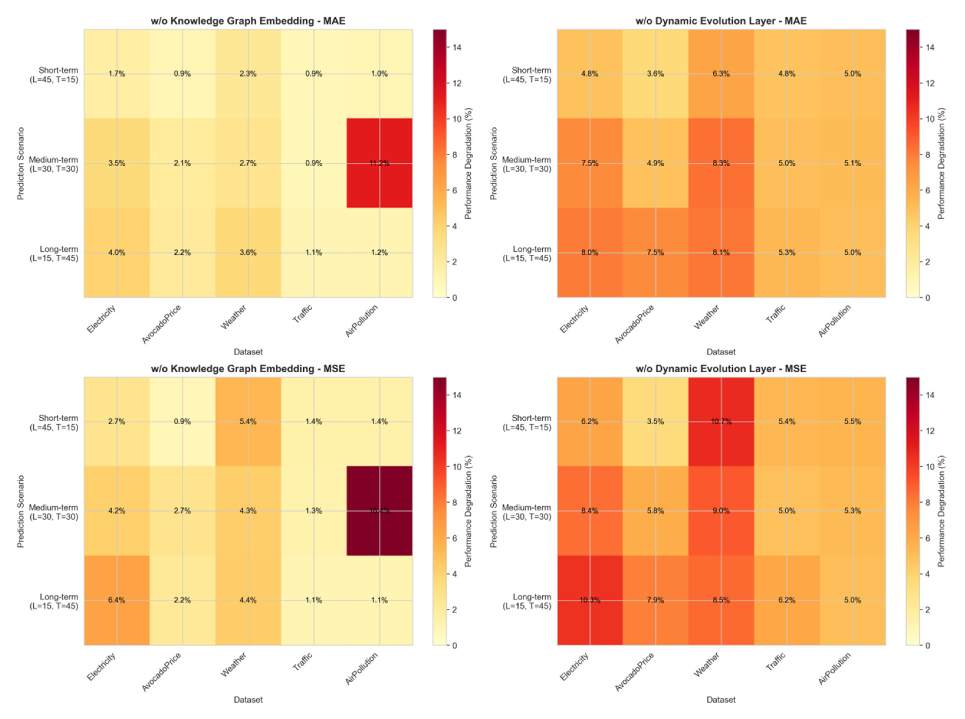
In short-term prediction scenarios, the impact of removing the knowledge graph embedding layer is minimal. For stationary sequences, the performance drops by approximately 1–2%. For non-stationary sequences, the performance drops by approximately 1%. This is in line with the description that “when making short-term predictions for stationary sequences, sequence models such as GRU can independently learn in this aspect, and thus the impact caused by knowledge graph embedding is relatively limited.”

In the medium-term prediction scenario, the role of the knowledge graph embedding layer lies between the short-term and long-term. The performance of stationary sequences drops by approximately 2–4%, while that of non-stationary sequences drops by about 1–2%.

In the long-term prediction scenario, after removing the knowledge graph embedding layer, the performance of stationary sequences (Electricity, AvocadoPrice, Weather) drops significantly (about 3–5%), while the performance of non-stationary sequences (Traffic, AirPollution) drops relatively less (about 1–2%). This is in line with the conclusion in the model description that “the performance of knowledge graph embedding algorithms is more significant when performing relatively stable sequence tasks that require long-term prediction.”

As shown in Table 3, Table 4 and Table 5, on all five datasets, after removing the knowledge graph embedding layer, all performance indicators of the model show a consistent and significant decline. This result strongly demonstrates the significant contribution of knowledge graph embedding to enhancing prediction accuracy. In conclusion, the embedding layer of a knowledge graph is not merely a simple information supplement. Instead, it endows the model with reasoning and semantic understanding capabilities by integrating sequential data with external knowledge, making its prediction results more interpretive and robust.

In short-term prediction scenarios, the impact of removing the dynamic evolution layer is relatively small (about 3–5%), but it is still greater than that of removing the knowledge graph embedding layer. This indicates that the dynamic evolution layer plays a fundamental role in sequence prediction.

In the mid-term prediction scenario, the removal of the dynamic evolution layer leads to a performance drop of approximately 4–7%. The ability of the dynamic evolution layer to capture the trend of sequence changes remains crucial in medium-term prediction.

The dynamic evolution layer is a core component of sequence prediction. After its removal, the performance of all datasets drops significantly (by approximately 5–8%). Long-term prediction tasks have higher requirements for the ability to capture sequence trends, so the performance degradation is more obvious.

As shown in Table 5, Table 6, Table 7 and Table 8, the results verify the rationality of the model design from another dimension. When the dynamic evolution layer was removed and only knowledge graph embeddings were used for prediction, the model’s performance on all datasets experienced a catastrophic decline, and its prediction error was even much higher than that of the ablation model in Scheme One. The core advantage of dynamic evolution layers (such as LSTM) lies in their ability to remember historical information and learn the complex dependencies between time steps. Removing it means that the model has completely lost its ability to learn “evolution”. It can only make predictions based on the inherent attributes of entities and is unable to answer dynamic questions such as “What is most likely to happen next under given historical conditions?”

The heat map likes Figure 10 shows the percentage decline in performance of the KD4SP model in different datasets and prediction scenarios after removing the knowledge graph embedding layer and the dynamic evolution layer. The depth of the color indicates the percentage of performance decline. The darker the color (red), the more significant the decline, and the more important this layer is. [X-axis] Five datasets (Electricity, AvocadoPrice, Traffic, Weather, AirPollution) [Y-axis] Three prediction scenarios (short-term L = 45, T = 15, medium-term L = 30, T = 30, long-term L = 15, T = 45).

Through the above two sets of ablation experiments in opposite directions, Scheme One (removing the knowledge graph embedding layer) proved that if the structured prior knowledge provided by the knowledge graph embedding is lacking, the model will degenerate into a pure sequence predictor, and its performance and generalization ability, especially when dealing with non-stationary data, will be significantly limited. Option Two (removing the dynamic layer) demonstrates that without the time series modeling capability provided by the dynamic evolution layer, the model is completely unable to understand the evolution law of the data over time, and the prediction task fundamentally cannot be carried out effectively.

The reason why the fusion model proposed in this study can achieve the best performance (as shown in the “Complete Model” column of each table) is precisely because it successfully integrates the advantages of both: the dynamic evolution layer is responsible for capturing the evolution patterns of data from the time dimension, while the knowledge graph embedding layer provides background knowledge and constraints for this evolution from the semantic dimension. The two complement each other and jointly form a powerful predictive framework that can both understand “when it occurs” and reason “why it occurs”. The ablation experiment not only quantitatively confirmed the necessity of each component, but also qualitatively revealed their irreplaceable roles in solving complex dynamic knowledge perception and prediction tasks.

The knowledge graph embedding layer plays a significant role in the long-term prediction tasks of stationary sequences, but its contribution is limited in the short-term prediction tasks of non-stationary sequences. This verifies the analysis in the model description regarding the applicable scenarios of the knowledge graph embedding algorithm. The dynamic evolution layer is a core component of sequence prediction and plays a crucial role in all prediction scenarios. Removing this layer will lead to a significant decline in model performance. The synergy of the two components enables the KD4SP model to maintain good prediction performance in different scenarios, especially in long-term prediction tasks of stationary sequences.

4.4. Experimental Results and Analysis

Each model adopted the mean absolute error (MAE) and mean square error (MSE) as evaluation indicators for performance evaluation. Both MAE and MSE are used as indicators to describe the degree of data fit, and are widely applied in sequence prediction tasks. Their calculation methods are depicted in Equations (33) and (34). K represents the sample size, and ${\mathrm{y}}_{\mathrm{k}}$ and ${\widehat{\mathrm{y}}}_{\mathrm{k}}$ represent the true value and predicted value, respectively. The smaller the calculated result, the better the performance of the model fitting.

$$\mathrm{M}\mathrm{A}\mathrm{E}={\displaystyle \frac{1}{K}}{\sum }_{k=1}^K\left|y_k-{\widehat{y}}_k\right|$$

(33)

$$\mathrm{M}\mathrm{S}\mathrm{E}={\displaystyle \frac{1}{K}}\sum _{k=1}^{\mathrm{K}}{(y_k-{\widehat{y}}_k)}^2$$

(34)

The LSTM–ATT–LSTM model adopted double-layer LSTM as the encoder and decoder [6]. An attention mechanism was introduced between the encoder and the decoder to precisely capture the key information in the input sequence. The AI-DTN model made corresponding changes or additions to the corresponding gating mechanism based on the GRU model [9]. The sequence information, target features, and auxiliary information were fully applied. The TCN model used causal convolution and scalable convolutional layers to handle time-series data [16]. The CNformer model proposed an encoder–decoder structure based on convolutional neural networks to capture the long-term dependencies in the time-series data [17]. The GEIFA model combined TCN, TransformerEncoder, and GCN to replace the traditional attention mechanism [18]. TCN was used to analyze time series, and TransformerEncoder served as the graph learner. The output of the encoder was input into the graph convolutional network GCN to extract the long-term features of the time series.

The model adopted in this study and the experimental environment of the above-mentioned model were all run under the Pytorch 2.5.1 deep learning framework in the model training stage. Generally, the model varies depending on the graphics cards. The graphics card adopted GPUT4 with 16 GB of video memory to ensure model efficiency. GPUT4 showed high performance and low latency when dealing with large neural network models, and was particularly suitable for deep learning tasks. The training rounds for each model were 50, and the training batches were 200. The Adam optimizer was adopted to optimize the loss function, with an initial learning rate of 1 × 10⁻⁴. The experimental hyperparameter settings of the KD4SP model are shown in

Table 9. KD4SP model parameters.

Parameter Interpretation	Parameter Value
Embedding dimension	64
Feature extraction layer and hidden layer	64
Dynamic evolution layer and hidden layer	64
Regularization coefficient of auxiliary loss function	1
Auxiliary loss function weights	0.1

. The size of the sliding window capacity of each dataset was set to 60, and the length of the historical sequence L and the length of the target sequence T were set for three rounds in the experimental preprocessing stage. Round One: Set L = 45 and T = 15. The experimental results of each model are shown in

Table 10. Experimental results of each model at L = 45 and T = 15.

	Electricity		Avocado Price		Traffic		Weather		Air Pollution
	MAE	MSE	MAE	MSE	MAE	MSE	MAE	MSE	MAE	MSE
LSTM–Att–LSTM	0.366	0.231	0.640	0.754	0.422	0.334	0.204	0.102	0.398	0.395
AI-DTN	0.411	0.327	0.688	0.789	0.451	0.368	0.203	0.924	0.430	0.425
TCN	0.480	0.417	0.773	0.891	0.566	0.534	0.251	0.157	0.485	0.497
CNformer	0.435	0.308	0.695	0.804	0.462	0.377	0.189	0.062	0.426	0.430
GEIFA	0.454	0.338	0.670	0.814	0.521	0.471	0.237	0.101	0.439	0.438
KD4SP	0.351	0.224	0.632	0.749	0.439	0.353	0.174	0.056	0.420	0.422

. Round Two: Set L = 30 and T = 30. The experimental results of each model are shown in

Table 11. Experimental results of each model at L = 30 and T = 30.

	Electricity		Avocado Price		Traffic		Weather		Air Pollution
	MAE	MSE	MAE	MSE	MAE	MSE	MAE	MSE	MAE	MSE
LSTM–Att–LSTM	0.405	0.288	0.748	1.038	0.568	0.531	0.315	0.198	0.534	0.588
AI-DTN	0.481	0.372	0.762	1.032	0.592	0.562	0.351	0.262	0.573	0.620
TCN	0.493	0.407	0.810	1.100	0.682	0.650	0.413	0.303	0.586	0.639
CNformer	0.466	0.361	0.758	0.982	0.588	0.563	0.296	0.194	0.539	0.601
GEIFA	0.469	0.366	0.744	0.951	0.640	0.643	0.386	0.285	0.548	0.615
KD4SP	0.398	0.286	0.713	0.943	0.576	0.543	0.300	0.188	0.544	0.608

. Round 3: Set L = 15 and T = 45. The experimental results of each model are shown in

Table 12. Experimental results of each model at L = 15 and T = 45.

	Electricity		Avocado Price		Traffic		Weather		Air Pollution
	MAE	MSE	MAE	MSE	MAE	MSE	MAE	MSE	MAE	MSE
LSTM–Att–LSTM	0.455	0.371	0.772	1.103	0.647	0.642	0.457	0.432	0.593	0.696
AI-DTN	0.524	0.434	0.804	1.102	0.690	0.714	0.486	0.514	0.630	0.743
TCN	0.569	0.487	0.862	1.221	0.761	0.814	0.527	0.533	0.625	0.735
CNformer	0.510	0.421	0.768	1.081	0.658	0.671	0.443	0.422	0.605	0.703
GEIFA	0.495	0.410	0.795	1.150	0.685	0.713	0.514	0.536	0.613	0.733
KD4SP	0.449	0.358	0.742	1.006	0.647	0.648	0.442	0.410	0.598	0.700

.

Both MAE and MSE are important indicators for sequence prediction. The fundamental difference lies in that MSE is more sensitive to errors than MAE. From the perspectives of variance, standard deviation, and ADF test, the results of the three experiments show that it is undeniable that the model has deficiencies in predicting non-stationary sequences. However, the performance advantage of KD4SP over other models in the scenario of stationary sequences is not completely invalid.

The analysis of the aforementioned experimental data showed that the KD4SP model performed better than the other models in the datasets Electricity, AvocadoPrice, and AirPollution. The performance of the KD4SP model in the datasets Traffic and AirPollution was inferior to that of the LSTM–Att–LSTM model. The length $\mathrm{T}\le 30$ of the target sequence indicated that the differences between the KD4SP and LSTM–Att–LSTM models gradually became obvious. Taking the dataset AirPollution as an example, the differences in MAE and MSE between the two increased from 0.6% and 0.3% in T = 45 to 2.2% and 2.7% in T = 15, respectively, indicating that the KD4SP model was inferior to the decoding model in handling short-term predictions. The performance of the hybrid models of the convolution module, such as the TCN, CNformer, and GEIFA models, was slightly inferior to that of the sequence prediction models. Given the overly complex nature of the models, the relatively small amount of training data was insufficient to support the improvement in their performance.

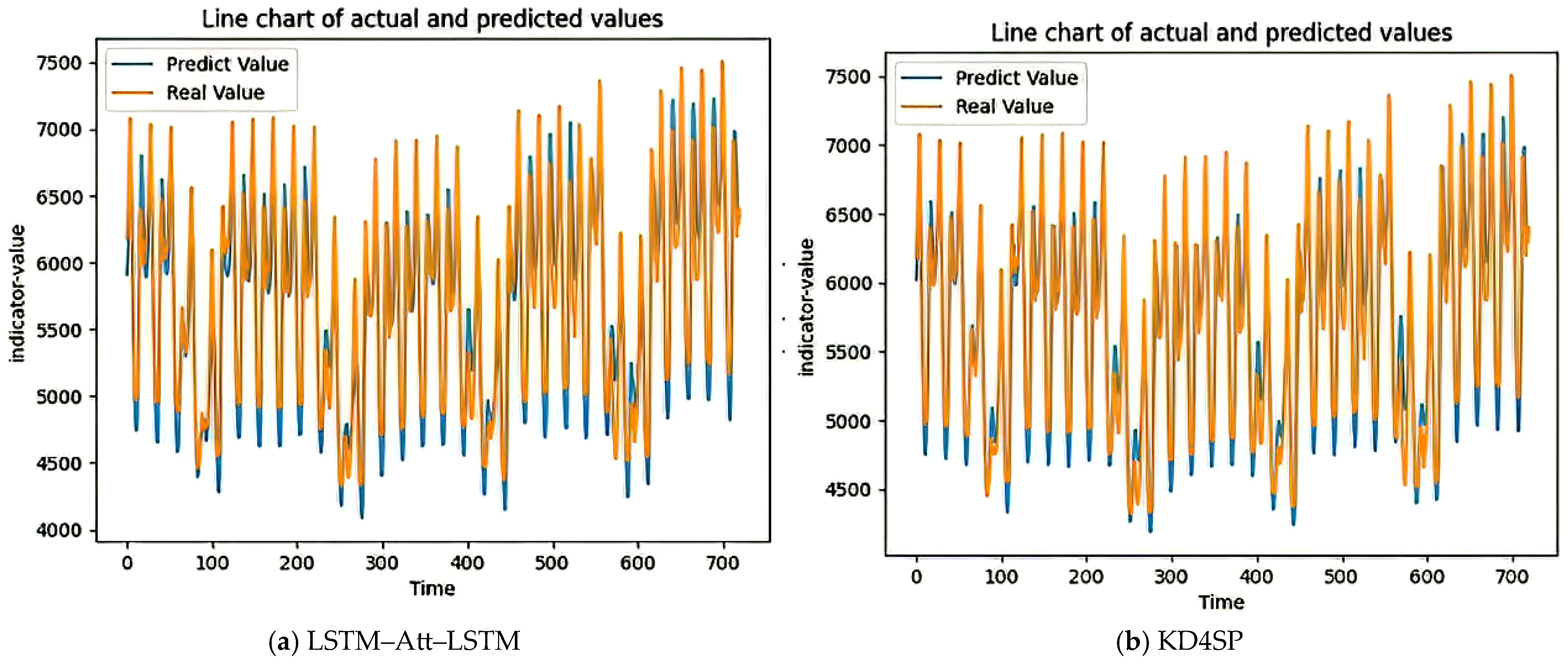
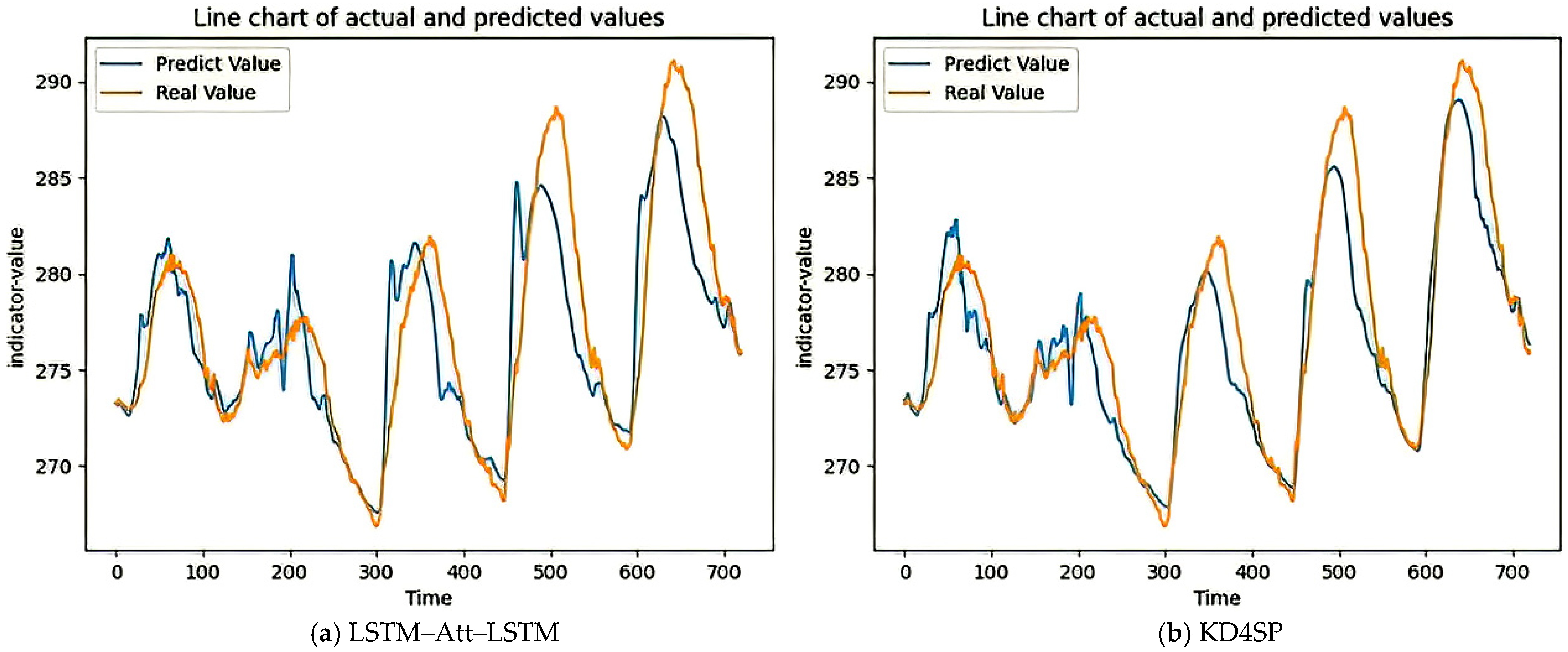
This study started from two aspects to track the differences between the LSTM–Att–LSTM and KD4SP algorithms: the influence of the predicted time step T on the model and the influence of the dataset on the model. In terms of the dataset, the length T = 45 of the target sequence was fixed first. The LSTM–Att–LSTM algorithm and the KD4SP algorithm were applied on the test sets of the datasets Electricity and Weather. Regarding the fitting between the predicted and true values, the first 720 steps of data were intercepted, as shown in Figure 11 and Figure 12. When the sequence data were relatively stable, that is, the dataset where the standard deviation of the predicted values is much smaller than the average value. The KD4SP model performed better than LSTM–Att–LSTM in terms of fitting. This was more obvious in the prediction of the Weather dataset. This was because data with smaller fluctuations had no high requirements for the complexity of the model. The attention mechanism of LSTM–Att–LSTM might have made it difficult for the model to learn effective weights due to the lack of significant feature differences.

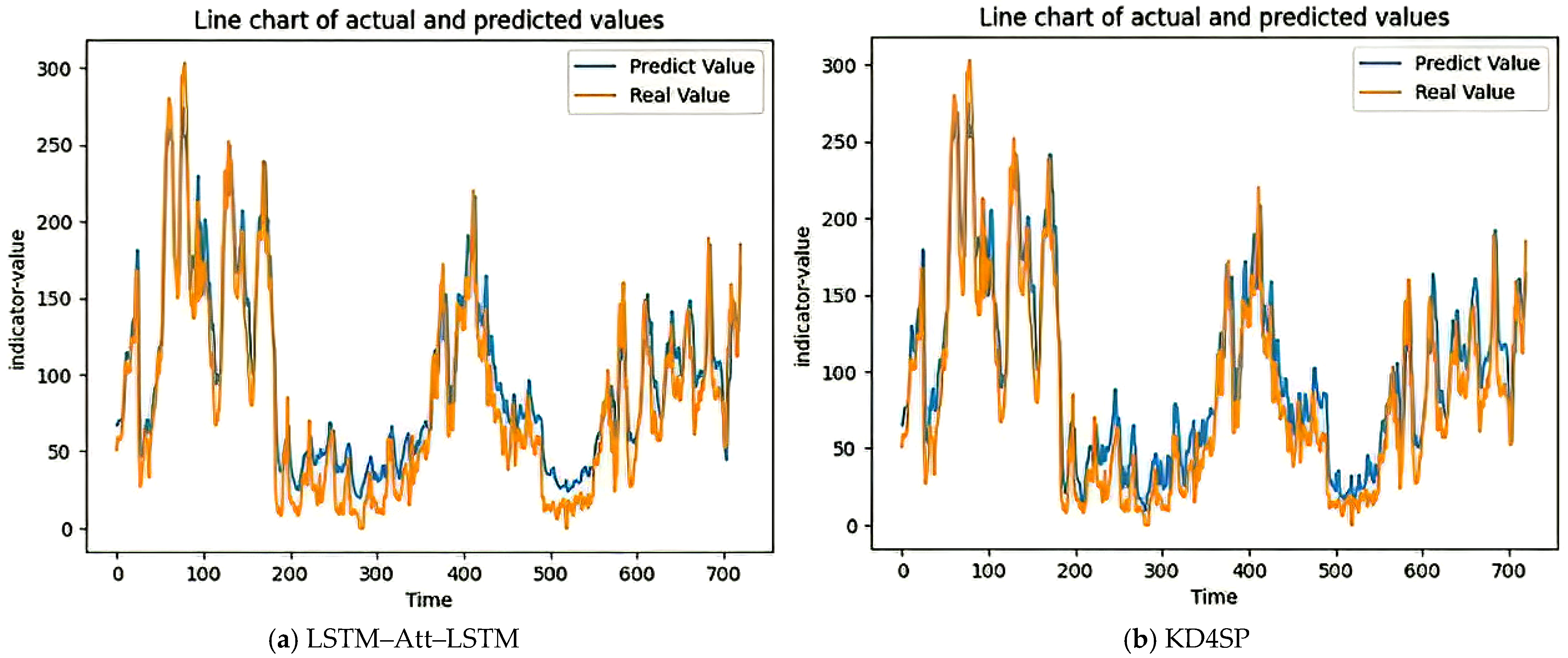
In terms of predicting the time step T, the dataset AirPollution was selected where the LSTM–Att–LSTM model performed better than the KD4SP model. The fitting situations of the predicted and true values of the validation sets of the two models were analyzed at T = 15 and T = 45, respectively. The fitting situations are shown in Figure 13 and Figure 14. The performance gap between the KD4SP model and the LSTM–Att–LSTM model gradually decreased with the increase in the prediction time step T. The fitting effect of the LSTM–Att–LSTM model was better than that of the KD4SP model in the time-step range of 500 to 550. When T increased to 45, no difference in the fitting effect was observed between the LSTM–Att–LSTM and KD4SP models. This was because the requirement for the prerequisite information of decoding accuracy gradually increased with the increase in the predicted time-step size, resulting in insufficient data support for decoding during model prediction.

The selection of hyperparameters has a crucial impact on the performance of the model in the research and application of machine learning and deep learning. This study involved an in-depth analysis of the influence of different hyperparameters on the experimental results, thereby seeking the key factors for optimizing the model performance.

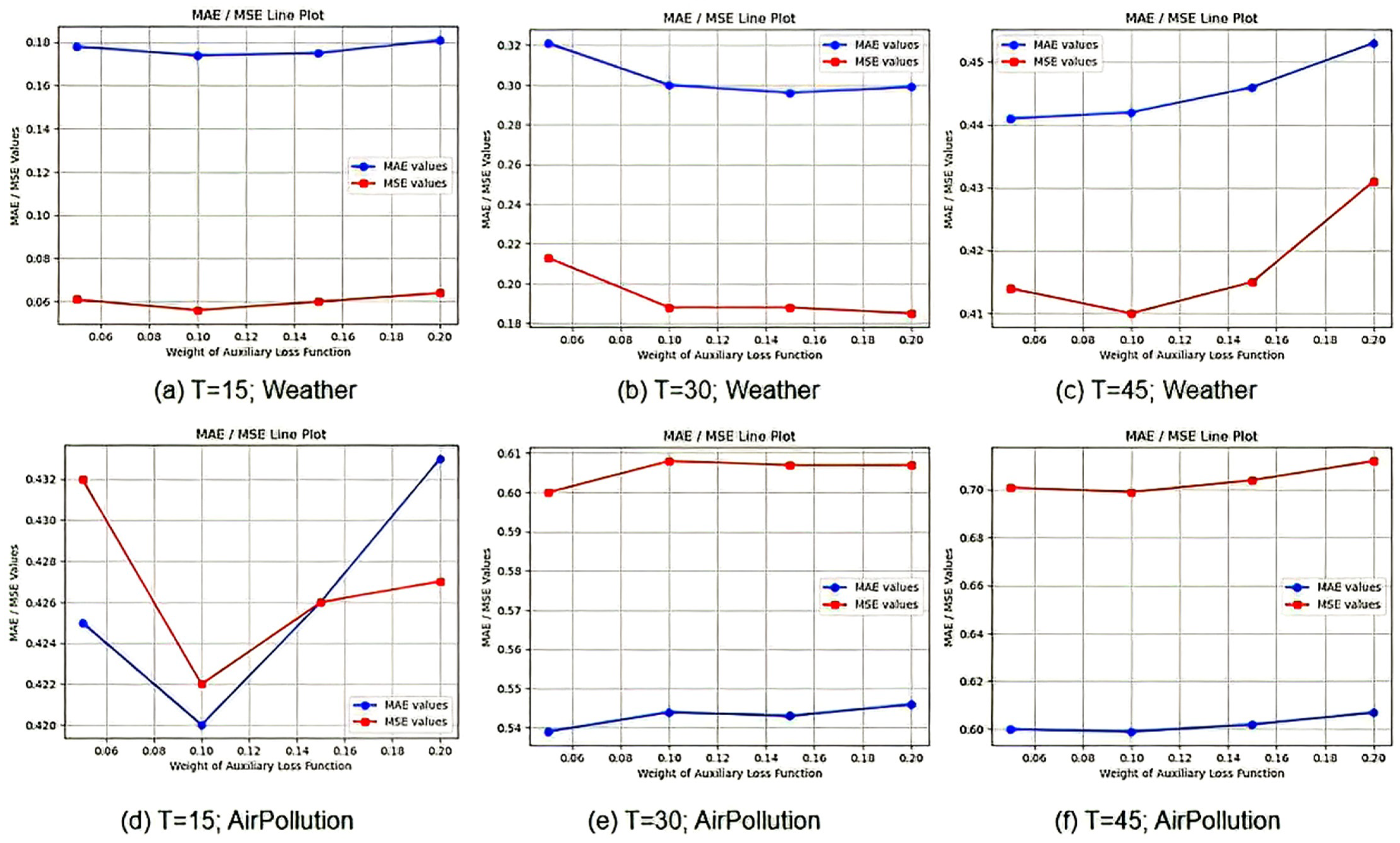
The index trends of MAE/MSE under different weights of the auxiliary loss function are shown in Figure 14. In most cases, the KD4SP model performed well when the weight of the auxiliary loss function was 0.1 for the datasets AirPollution and Weather. The auxiliary loss function mainly serves to assist in optimizing the model and is applicable to models with multiple subframes. The training dataset Weather showed that when the predicted time step T = 15, no significant changes occurred in each index. When T = 30, it showed that when the weight of the auxiliary loss function was $\mathsf{\gamma }\ge 0.1$, each index gradually stabilized, whereas when T = 45, it presented a concave curve centered on $\mathsf{\gamma }=0.1$. The dataset AirPollution showed that when the predicted time step was T = 15, the model achieved the best result at $\mathsf{\gamma }=0.1$. However, when $\mathrm{T}\ge 30$, the larger the value of $\mathsf{\gamma }$, the lower the performance of the model.

For datasets with relatively stable sequences, when the prediction time step was large, the model was more sensitive to changes in auxiliary losses. For datasets with unstable sequences, when the prediction time step was small, the auxiliary loss was likely to be advantageous. This was because when making short-term predictions for non-stationary sequences, the auxiliary loss suppressed the interference of burst noise and prevented the model from overfitting. However, when making long-term predictions, significant fluctuations in the data dominated the errors and weakened the correction effect of auxiliary information. When making short-term predictions for stationary sequences, sequence models such as GRU could learn independently in this aspect. Therefore, the impact caused by knowledge graph embedding was relatively limited.

As shown in Figure 15, Long-term prediction requires models to provide structured knowledge to ensure the accuracy of the prediction. Under normal circumstances, the auxiliary loss occupying a high position, especially in the knowledge graph embedding algorithm, is not desirable. A high auxiliary loss leads to the overuse of the knowledge graph embedding algorithm by the model, deviating from the purpose of sequence prediction and resulting in a decline in the model’s prediction performance. These findings indicated that the performance of the knowledge graph embedding algorithm was more significant when performing sequential tasks that were relatively stable and required long-term prediction. The size of the auxiliary loss weight also needed to be adjusted properly so as not to deviate from the purpose of sequence prediction.

The performance of the sequence prediction model proposed in this paper, which integrates knowledge graph embedding and dynamic evolution, is not constant but is profoundly influenced by the knowledge graph itself, the characteristics of sequence data, and the stability of the dataset. An in-depth exploration of these factors is crucial for understanding the advantages and limitations of the model and guiding its application scenarios.

First of all, the scale and quality of the knowledge graph are the basis for determining the performance of the model. A large-scale, high-quality knowledge graph rich in entities and relationships can provide rich semantic context for sequential data, greatly enhancing the model’s relational reasoning ability and interpretability. For instance, in traffic prediction, a graph that contains diverse information such as road grades, real-time events, and weather impacts can help the model more accurately analyze the causes of congestion. However, “big” does not always equate to “good”. When the scale of the graph is too large but contains a large number of redundant relationships irrelevant to the current prediction task, the model will not only bear a huge computational burden, but also may introduce noise, causing the attention mechanism to be dispersed, thereby reducing the prediction accuracy. Therefore, the information density and task relevance of the graph are more crucial indicators than simple scale.

Secondly, the sequence length and the stability of the dataset jointly determine the effectiveness of the dynamic evolution module. For long-term and stable sequences (such as power load data with obvious seasonality), the model can clearly capture reliable periodic and trend patterns from long historical sequences through dynamic evolution layers. At this point, the knowledge graph embedding is responsible for providing macroscopic and structured background knowledge (such as the impact of holiday types on power consumption patterns). The two work together, and the model performance is usually excellent. On the contrary, when confronted with short sequences or highly non-stationary data (such as stock price data that is severely affected by breaking news), the dynamic evolution layer finds it difficult to learn stable evolution patterns from the limited history. At this point, the model will rely more on the static inherent relationships among entities in the knowledge graph (such as the industry to which the company belongs and supply chain associations) for reasoning, and the contribution of dynamic evolution will be relatively weakened. If the knowledge graph fails to incorporate key event-based knowledge (such as policy changes), the model will perform poorly in the face of sharp fluctuations.

In conclusion, the performance advantage of this fusion model lies in its ability to collaboratively utilize structured knowledge (graphs) and dynamic patterns (evolution). The scenarios where it performs better are usually: the knowledge graph is well-constructed, highly relevant to the task, and the sequence is long enough for the model to recognize the evolution pattern. However, when the noise in the graph is too large, the sequence is too short, or the data distribution undergoes drastic changes, the performance of the model will be affected. This analysis indicates that future research should focus on developing adaptive graph pruning mechanisms and dynamic evolutionary algorithms that are more robust to non-stationarity, in order to further enhance the universality and robustness of the model in the complex real world.

For datasets with relatively stable sequences, when the prediction time step is large, the model is more sensitive to changes in auxiliary losses. For datasets with unstable sequences, the auxiliary loss can only play an advantage when the prediction time step is relatively small. The possible reasons for this are as follows: When making short-term predictions for non-stationary sequences, the auxiliary loss can suppress the interference of sudden noise and prevent overfitting of the model. However, when making long-term predictions, the significant fluctuations in data will dominate the error and weaken the correction effect of the auxiliary information. When making short-term predictions for stationary sequences, sequence models such as GRU can independently learn in this aspect, so the impact caused by knowledge graph embedding is relatively limited. However, long-term predictions require models to provide structured knowledge to ensure the accuracy of the predictions. However, it is worth noting that in general, it is not desirable for the auxiliary loss to occupy a high position, especially in knowledge graph embedding algorithms. A high auxiliary loss will lead the model to overuse the knowledge graph embedding algorithm and deviate from the purpose of sequence prediction, resulting in a decline in the model’s prediction performance.

By comparing the KD4SP models without knowledge graph embedding, without dynamic evolution, and both, it is found that knowledge graph embedding and dynamic evolution each play different roles in enhancing the model’s performance. The former enhances the model’s context understanding ability, while the latter provides a flexible temporal reasoning mechanism. The combination of the two enables the KD4SP model to play their respective unique roles when dealing with complex time series prediction tasks.

5. Conclusions and Discussion

Aiming at the problems such as insufficient modeling ability of long sequence dependencies, lack of interpretability, and low efficiency of multi-element heterogeneous information fusion in sequence prediction models, this study proposed a sequence prediction framework integrating knowledge graph embedding and dynamic evolution. The context information of the sequence was captured to improve the accuracy of sequence prediction. Experiments were conducted using five datasets from different application fields to verify the validity of the model. The experimental results showed that the KD4SP model improved the expression performance of stationary sequences compared with algorithms of the same type, under the condition that the size of the prediction time step was the same. Given its certain limitations in the sequence prediction task, the knowledge graph embedding model still relies on the weight distribution of knowledge graph embedding and dynamic evolution when facing different datasets. Therefore, a future research direction is to enhance the efficiency of integrating knowledge graphs into sequence prediction.

Based on the sequence prediction framework integrating knowledge graph embedding and dynamic evolution proposed in this paper, future research can be further deepened in the following three key dimensions to enhance the adaptability, scalability and practicality of the model:

Firstly, introducing an adaptive attention weight distribution strategy into the dynamic evolution mechanism is an important direction for improving the accuracy of the model. The current model needs to manually adjust the weights of knowledge graph embedding and dynamic evolution when dealing with data from different domains. In the future, an adaptive weight module based on data features (such as sequence volatility, relationship density) or task objectives (such as long-term prediction and short-term prediction) can be designed, enabling the model to independently determine when to rely on semantic relationships in the graph and when to focus on temporal dynamic changes. So as to achieve more refined evolutionary modeling in complex scenarios.

Secondly, efforts should be made to promote the automation of knowledge graph construction and update to enhance the transferability of models in cross-domain tasks. At present, the construction of graphs mostly relies on manual priors, which limits the rapid deployment of models in new scenarios. In the future, methods for automatically extracting entities and relationships from sequential data and dynamically expanding the graph structure can be explored. Combined with meta-learning or transfer learning mechanisms, the model can quickly adapt to new fields based on a small number of samples (such as migrating from traffic prediction to medical monitoring), reducing the reliance on complete knowledge graphs.

Finally, to enhance the practical value of the framework, it is necessary to focus on strengthening its cross-domain generalization ability. Although the current model has demonstrated good performance on data from multiple fields such as power, transportation, and weather, its robustness to heterogeneous data distribution and different semantic relationship types should be further explored in the future. For instance, a cross-domain unified dynamic evolution representation framework can be constructed to enable the knowledge reasoning and temporal evolution modules to have domain-independent feature interaction capabilities, thereby supporting the effective transfer from stationary sequences (such as electricity prices) to non-stationary sequences (such as emergency visit volumes) without retraining.

Through continuous exploration in the above-mentioned directions, the sequence prediction framework that integrates knowledge graphs and dynamic evolution is expected to achieve a better balance among interpretability, adaptability and computational efficiency, and ultimately realize reliable deployment in complex real-world scenarios.

References

1. Bie, Y. Research on Space-Time Feature Learning Method for Short-Term and Near-Term Precipitation Radar Echo Sequence Prediction. Master’s Thesis, Xi’an University of Technology (China), Xi’an, China, 2023. [Google Scholar]
2. Zhu, Z.; Tang, C. Multi-site PM2.5 mass concentration prediction method based on GCN-GRU-Attention. J. Hubei Minzu Univ. 2025, 43, 67–72+85. [Google Scholar] [CrossRef]
3. Li, T.; Wang, T.; Zhang, Y. Consider the multi-feature expressway traffic flow prediction model. Transp. Syst. Eng. Inf. 2021, 21, 101–111. [Google Scholar] [CrossRef]
4. Spiliotis, E. Decision trees for time-series forecasting. Foresight 2022, 1, 30–44. [Google Scholar]
5. Pattanayak, R.M.; Panigrahi, S.; Behera, H.S. High-order fuzzy time series forecasting by using membership values along with data and support vector machine. Arab. J. Sci. Eng. 2020, 45, 10311–10325. [Google Scholar] [CrossRef]
6. Wen, X.; Li, W. Time Series Prediction Based on LSTM-Attention-LSTM Model. IEEE Access 2023, 11, 48322–48331. [Google Scholar] [CrossRef]
7. Chen, G.; Tian, H.; Xiao, T.; Xu, T.; Lei, H. Time series forecasting of oil production in Enhanced Oil Recovery system based on a novel CNN-GRU neural network. Geoenergy Sci. Eng. 2024, 233, 212528. [Google Scholar] [CrossRef]
8. Rostamian, A.; O’hara, J.G. Event prediction within directional change framework using a CNN-LSTM model. Neural Comput. Appl. 2022, 34, 17193–17205. [Google Scholar] [CrossRef]
9. Wang, Y.; Feng, S.; Wang, B.O.J. Deep transition network with gating mechanism for multivariate time series forecasting. Appl. Intell. Int. J. Artif. Intell. Neural Netw. Complex Probl.-Solving Technol. 2023, 53, 24346–24359. [Google Scholar] [CrossRef]
10. Chen, Y.; Ding, F.; Zhai, L. Multi-scale temporal features extraction based graph convolutional network with attention for multivariate time series prediction. Expert Syst. Appl. 2022, 200, 117011. [Google Scholar] [CrossRef]
11. Yu, X.; Shi, S.; Xu, L. A spatial—Temporal graph attention network approach for air temperature forecasting. Appl. Soft Comput. 2021, 113, 107888. [Google Scholar] [CrossRef]
12. Zhu, C. Deep User Interest Evolution Model Based on Graph Data Enhancement. Master’s Thesis, Shanxi University, Taiyuan, China, 2023. [Google Scholar]
13. Saxena, A.; Kochsiek, A.; Gemulla, R. Sequence-to-Sequence Knowledge Graph Completion and Question Answering. arXiv 2022. [Google Scholar] [CrossRef]
14. Hu, Z. Behavior Prediction and Sequence Recommendation Based on User Interaction Intentions. Master’s Thesis, Qinghai Normal University, Xining, China, 2024. [Google Scholar] [CrossRef]
15. Ge, X.; Wang, Y.C.; Wang, B.; Kuo, C.C.J. Knowledge Graph Embedding: An Overview. arXiv 2023, arXiv:2309.12501. [Google Scholar] [CrossRef]
16. Liu, J.; Ma, T.; Su, Y. Polynomial projection and information exchange architecture for long-term Time series prediction. Comput. Eng. Appl. 2025, 61, 120. Available online: http://kns.cnki.net/kcms/detail/11.2127.tp.20240621.0915.002.html (accessed on 12 May 2025).
17. Wang, X.; Liu, H.; Yang, Z.; Du, J.; Dong, X. CNformer: A convolutional Transformer with decomposition for long-term multivariate time series forecasting. Appl. Intell. 2023, 53, 20191–20205. [Google Scholar] [CrossRef]
18. Wu, Q. Multivariate time series prediction based on deep learning. J. Nanjing Univ. Financ. Econ. 2024. [Google Scholar] [CrossRef]
19. Xie, G.; Shangguan, A.; Fei, R.; Ji, W.; Ma, W.; Hei, X. Motion trajectory prediction based on a CNN-LSTM sequential model. Sci. China Inf. Sci. 2020, 63, 212207. [Google Scholar] [CrossRef]
20. Wan, R.; Mei, S.; Wang, J.; Liu, M.; Yang, F. Multivariate temporal convolutional network: A deep neural networks approach for multivariate time series forecasting. Electronics 2019, 8, 876. [Google Scholar] [CrossRef]
21. Hao, J. Research on Time Series Prediction Algorithm Based on Deep Learning. Master’s Thesis, Shandong Normal University, Jinan, China, 2024. [Google Scholar] [CrossRef]
22. Wu, Z.; Pan, S.; Chen, F.; Long, G.; Zhang, C.; Yu, P.S. A comprehensive survey on graph neural networks. IEEE Trans. Neural Netw. Learn. Syst. 2020, 32, 4–24. [Google Scholar] [CrossRef] [PubMed]
23. Jiang, W.; Luo, J.; He, M.; Gu, W. Graph neural network for traffic forecasting: The research progress. ISPRS Int. J. Geo-Inf. 2023, 12, 100. [Google Scholar] [CrossRef]
24. Li, Z.; Huang, B.; Wang, C. Meta-path recommendation algorithm for knowledge graph embedding based on heterogeneous attention networks. J. Univ. Electron. Sci. Technol. China 2025, 54, 776–788. Available online: http://kns.cnki.net/kcms/detail/51.1207.TN.20241225.2003.004.html (accessed on 25 March 2025).
25. Electricity. Available online: https://archive.ics.uci.edu/ml/datasets/individual+household+electric+power+consumption (accessed on 7 December 2025).
26. Cheng, S. Research and Implementation of Movie Recommendation System Based on Deep Learning and Behavior Sequence. Master’s Thesis, Southwest Jiaotong University, Chengdu, China, 2022. [Google Scholar]
27. Avocado Price. Available online: https://www.kaggle.com/datasets/neuromusic/avocado-prices (accessed on 7 December 2025).
28. Zhou, G.; Zhu, X.; Song, C.; Fan, Y.; Zhu, H.; Ma, X.; Yan, Y.; Jin, J.; Li, H.; Gai, K. Deep Interest Network for Click-Through Rate Prediction. In Proceedings of the 24th ACM SIGKDD International Conference on Knowledge Discovery and Data Mining, London, UK, 19–23 August 2018; pp. 1059–1068. [Google Scholar] [CrossRef]
29. Traffic. Collected, organized and released by an authoritative data storage platform named “UCI Machine Learning Repository” (University of California, Irvine Machine Learning Repository). Available online: https://archive.ics.uci.edu/ml/datasets/PEMS-SF (accessed on 7 December 2025).
30. Bai, S.; Kolter, J.Z.; Koltun, V. An empirical evaluation of generic convolutional and recurrent networks for sequence modeling. In Proceedings of the International Conference on Learning Representations, Vancouver, BC, Canada, 30 April–3 May 2018. [Google Scholar]
31. Weather. Weather.js is designed as a comprehensive JavaScript Weather library built around the OpenWeatherMap API (non-affiliate relationship), originally created by Noah Smith and currently maintained by PallasStreams. Available online: https://github.com/noazark/weather (accessed on 7 December 2025).
32. AirPollution. A Well-Known Multivariate Time Series Benchmark Dataset Collated and Published by the UCI Machine Learning Repository. Available online: https://archive.ics.uci.edu/ml/datasets/Air+Quality (accessed on 7 December 2025).
Figure 1. Spatial position of the TransE model.
Electronics 14 04922 g001
Figure 2. Spatial position of the TransH model.
Electronics 14 04922 g002
Figure 3. Spatial mapping diagrams of the TransH and TransR models.
Electronics 14 04922 g003
Figure 4. Schematic diagram of the interest evolution layer of the DIEN model.
Electronics 14 04922 g004
Figure 5. GAT information transmission process of the DySAT model.
Electronics 14 04922 g005
Figure 6. KD4SP algorithm model framework.
Electronics 14 04922 g006
Figure 7. Schematic diagram of GRU model architecture.
Electronics 14 04922 g007
Figure 8. Schematic diagram of the dynamic evolution framework of the KD4SP algorithm.
Electronics 14 04922 g008
Figure 9. Schematic diagrams of ReLU, LeakyReLU, and Dice.
Electronics 14 04922 g009
Figure 10. Heat map.
Electronics 14 04922 g010
Figure 11. Fitting comparison on the Electricity dataset.
Electronics 14 04922 g011
Figure 12. Fitting comparison on the Weather dataset.
Electronics 14 04922 g012
Figure 13. Fitting comparison on the AirPollution dataset (T = 15).
Electronics 14 04922 g013
Figure 14. Fitting comparison on the AirPollution dataset (T = 45).
Electronics 14 04922 g014
Figure 15. Index trend of MAE/MSE under different weights of the auxiliary loss function.
Electronics 14 04922 g015