Figure 1.
Global distribution of haiku as a literary form. International contests and workshops are held across Europe, North America, and Southeast Asia, reflecting its cultural diffusion.
Figure 1.
Global distribution of haiku as a literary form. International contests and workshops are held across Europe, North America, and Southeast Asia, reflecting its cultural diffusion.
Figure 2.
Example image generated by DALL·E for the haiku (English translation), “An old pond, a frog jumps in, the sound of water.” The visual output successfully captures the poem’s tranquil and introspective atmosphere.
Figure 2.
Example image generated by DALL·E for the haiku (English translation), “An old pond, a frog jumps in, the sound of water.” The visual output successfully captures the poem’s tranquil and introspective atmosphere.
Figure 3.
Distribution of normalized Valence, Energy, and Dynamism features. The balanced bell-shaped distributions indicate numerical stability and unbiased extraction.
Figure 3.
Distribution of normalized Valence, Energy, and Dynamism features. The balanced bell-shaped distributions indicate numerical stability and unbiased extraction.
Figure 4.
Spearman correlation heatmap among normalized Valence, Energy, and Dynamism features. Valence is strongly negatively correlated with Energy and Dynamism, while Energy and Dynamism are moderately positively correlated, indicating a structured and interpretable affective space rather than independent dimensions.
Figure 5.
Seasonal variation of normalized Valence, Energy, and Dynamism features. Each boxplot represents one of six kigo categories: Spring, Summer, Autumn, Winter, New Year, and All Year. Higher Valence and Energy appear in Spring and Summer, while New Year haiku show intermediate levels between Winter and Spring.
Figure 6.
Silhouette scores for different cluster numbers ( to 8) using k-means clustering.
Figure 6.
Silhouette scores for different cluster numbers ( to 8) using k-means clustering.
Figure 7.
Silhouette scores for different cluster numbers ( to 8) using Ward hierarchical clustering.
Figure 7.
Silhouette scores for different cluster numbers ( to 8) using Ward hierarchical clustering.
Figure 8.
3-D visualization of haiku distribution in the VED feature space. Colors denote k-means cluster assignments (). Cluster 0 corresponds to calm/positive haiku, and Cluster 1 to dramatic/active haiku with high expressive intensity.
Figure 8.
3-D visualization of haiku distribution in the VED feature space. Colors denote k-means cluster assignments (). Cluster 0 corresponds to calm/positive haiku, and Cluster 1 to dramatic/active haiku with high expressive intensity.
Figure 9.
2-D projections of the haiku VED feature space. The separation between clusters reflects affective differences in polarity (Valence) and intensity (Energy/Dynamism).
Figure 9.
2-D projections of the haiku VED feature space. The separation between clusters reflects affective differences in polarity (Valence) and intensity (Energy/Dynamism).
Figure 10.
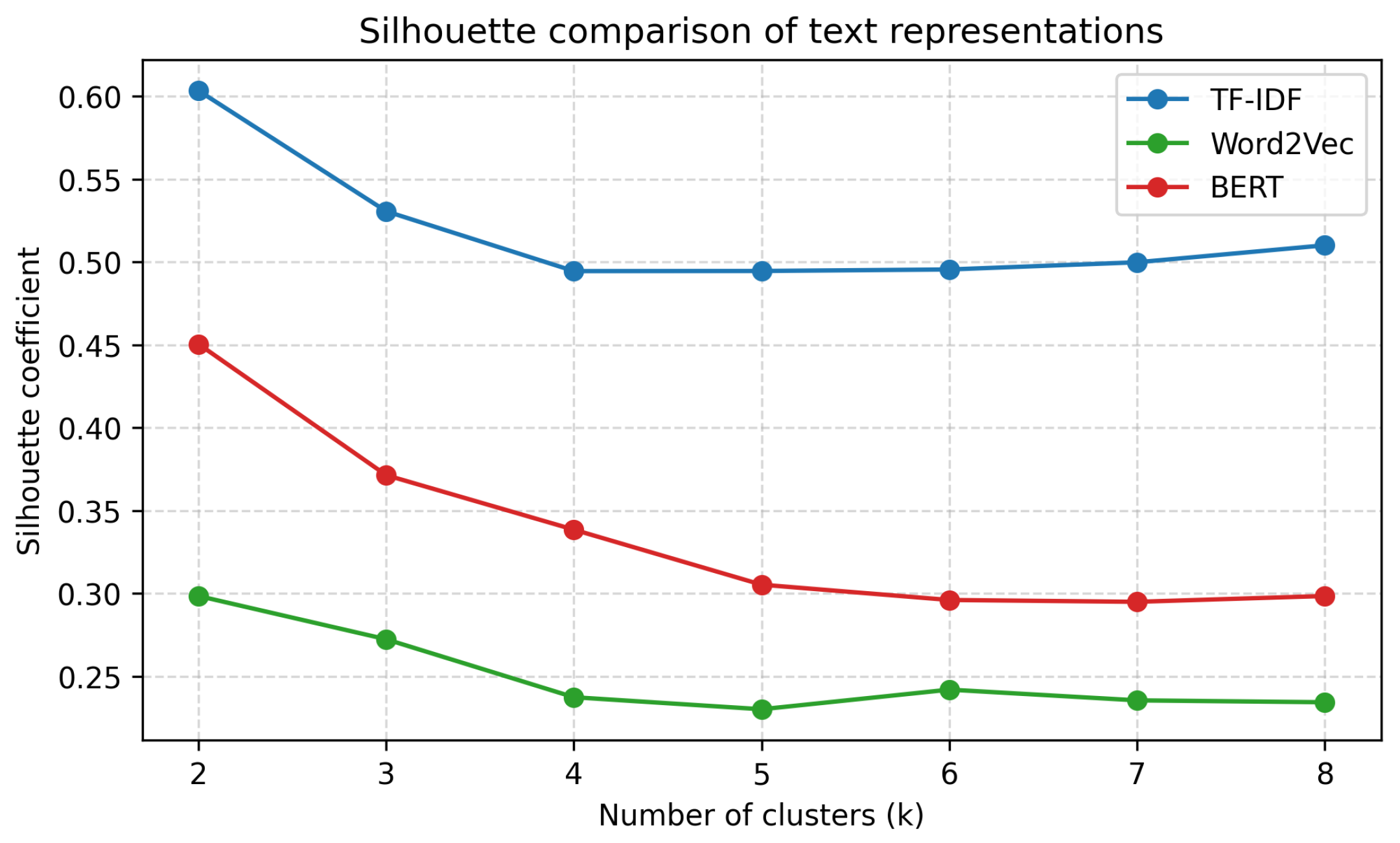
Comparison of silhouette coefficients across TF-IDF, Word2Vec, and BERT embeddings ( to 8).
Figure 10.
Comparison of silhouette coefficients across TF-IDF, Word2Vec, and BERT embeddings ( to 8).
Figure 11.
Two-dimensional PCA visualization of haiku embeddings based on TF-IDF (left), Word2Vec (middle), and BERT (right). Each point represents one haiku.
Figure 11.
Two-dimensional PCA visualization of haiku embeddings based on TF-IDF (left), Word2Vec (middle), and BERT (right). Each point represents one haiku.
Figure 12.
Distribution of normalized Valence, Energy, and Dynamism across two clusters () for each model.
Figure 12.
Distribution of normalized Valence, Energy, and Dynamism across two clusters () for each model.
Figure 13.
Seasonal means of Valence, Energy, and Dynamism for TF-IDF and BERT encoders.
Figure 13.
Seasonal means of Valence, Energy, and Dynamism for TF-IDF and BERT encoders.
Figure 14.
Overall distributions of four representative musical descriptors after robust normalization: (1) Tempo (BPM), (2) RMS Energy, (3) Spectral Centroid (Hz), and (4) Spectral Contrast (dB). Each feature was clipped to the 1st–99th percentile and rescaled to the range. The distributions are smooth and balanced, indicating numerically stable feature extraction.
Figure 15.
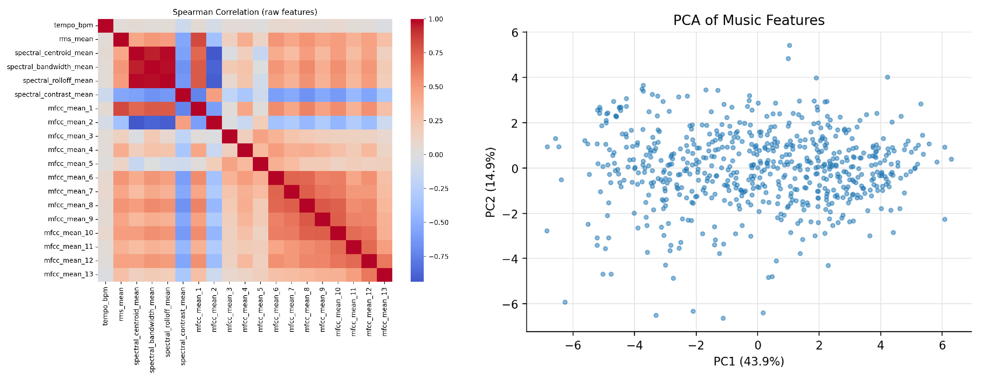
(Left) Spearman correlation heatmap among acoustic features, showing high internal consistency. (Right) PCA scatter plot, where PC1 corresponds to the Energy–Brightness axis and PC2 to the Tempo–Contrast axis, explaining about 67% of total variance.
Figure 15.
(Left) Spearman correlation heatmap among acoustic features, showing high internal consistency. (Right) PCA scatter plot, where PC1 corresponds to the Energy–Brightness axis and PC2 to the Tempo–Contrast axis, explaining about 67% of total variance.
Figure 16.
Silhouette scores for different cluster numbers ( to 8) using k-means clustering. The highest silhouette value (0.31) is obtained at , indicating that a three-cluster configuration best represents the underlying emotional structure.
Figure 16.
Silhouette scores for different cluster numbers ( to 8) using k-means clustering. The highest silhouette value (0.31) is obtained at , indicating that a three-cluster configuration best represents the underlying emotional structure.
Figure 17.
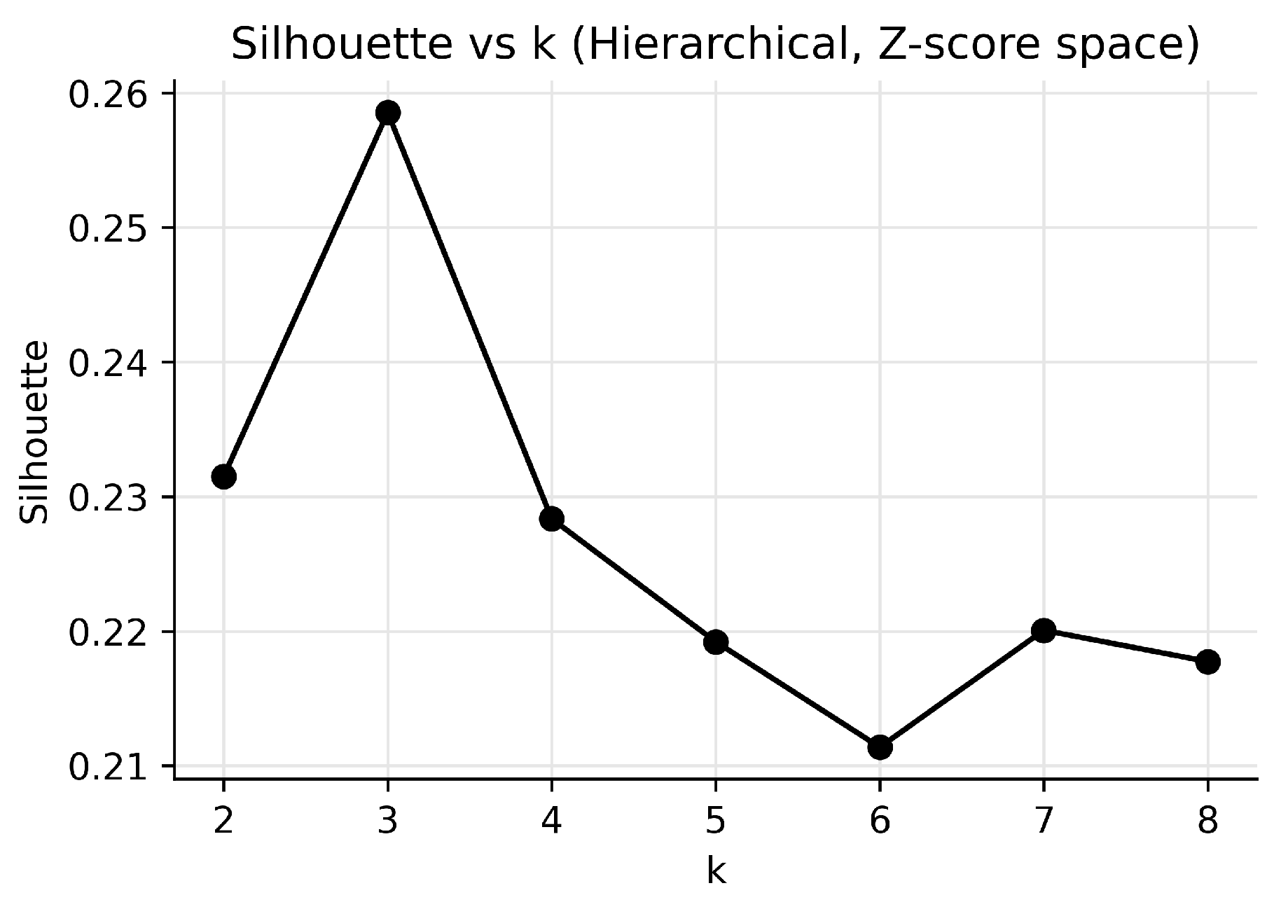
Silhouette scores for different cluster numbers ( to 8) using Ward hierarchical clustering. The highest silhouette value is obtained at , indicating that a three-cluster configuration provides the best structure under this method.
Figure 17.
Silhouette scores for different cluster numbers ( to 8) using Ward hierarchical clustering. The highest silhouette value is obtained at , indicating that a three-cluster configuration provides the best structure under this method.
Figure 18.
Clustering results projected onto Valence–Energy, Valence–Tempo, and Energy–Tempo planes. Each point represents one music piece; color indicates cluster membership (, silhouette = 0.31).
Figure 18.
Clustering results projected onto Valence–Energy, Valence–Tempo, and Energy–Tempo planes. Each point represents one music piece; color indicates cluster membership (, silhouette = 0.31).
Figure 19.
Axis-wise haiku–music alignment (Experiment D-1). Scatter plots for Valence, Energy, and Dynamism/Tempo show diagonal tendencies, indicating high cross-modal consistency. The displayed r values correspond to the empirical correlations of the matched pairs.
Figure 19.
Axis-wise haiku–music alignment (Experiment D-1). Scatter plots for Valence, Energy, and Dynamism/Tempo show diagonal tendencies, indicating high cross-modal consistency. The displayed r values correspond to the empirical correlations of the matched pairs.
Figure 20.
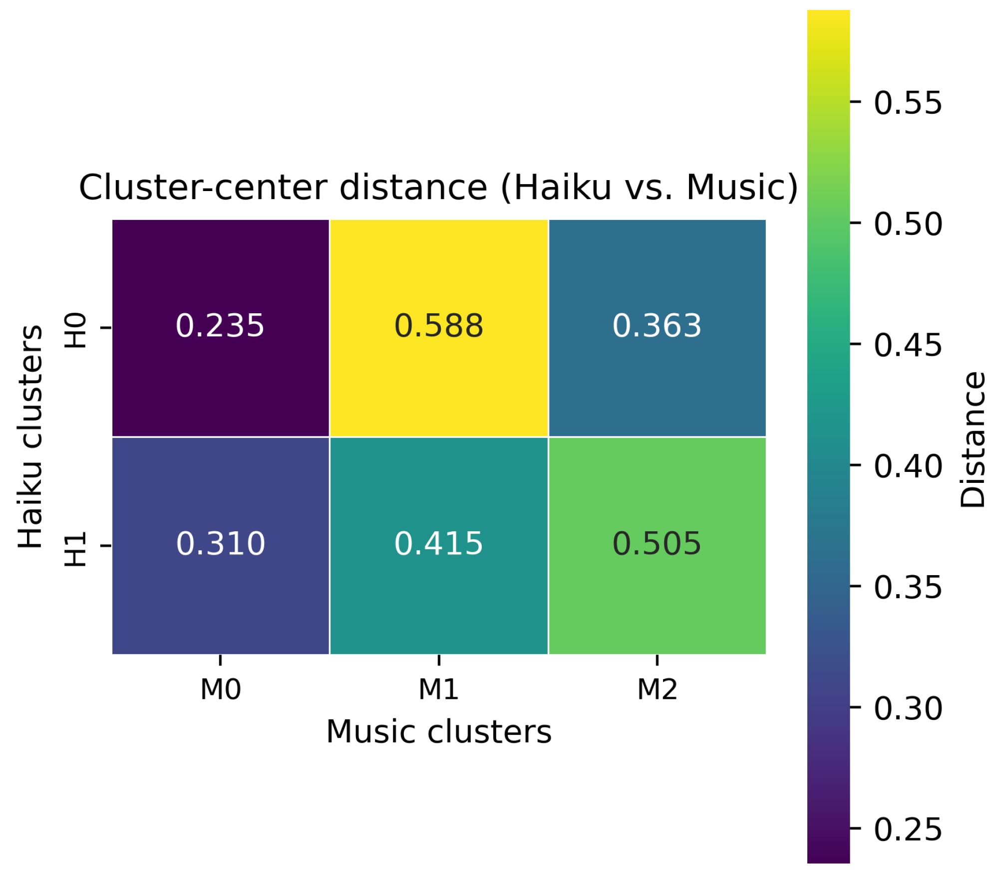
Cluster-center distances between haiku and music clusters (Experiment D-2). Each cell shows the Euclidean distance between a haiku cluster centroid and a music cluster centroid in the normalized affective space . Lower values indicate closer affective positions.
Figure 20.
Cluster-center distances between haiku and music clusters (Experiment D-2). Each cell shows the Euclidean distance between a haiku cluster centroid and a music cluster centroid in the normalized affective space . Lower values indicate closer affective positions.
Figure 21.
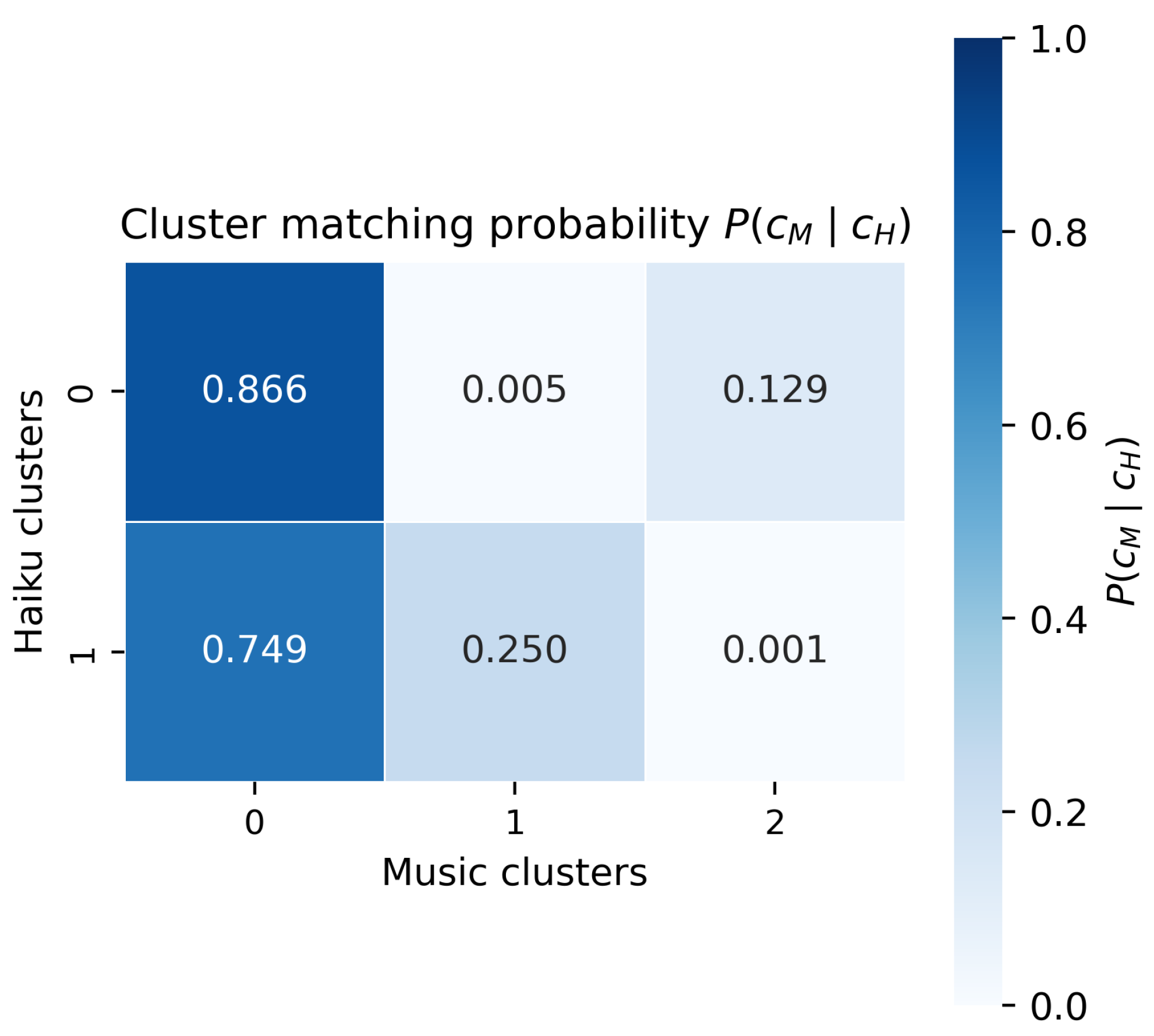
Cluster matching probabilities (Experiment D-2). Each cell shows the conditional probability that a haiku from cluster is matched to music from cluster , based on the 1067 haiku–music pairs. Darker cells indicate higher matching probability.
Figure 21.
Cluster matching probabilities (Experiment D-2). Each cell shows the conditional probability that a haiku from cluster is matched to music from cluster , based on the 1067 haiku–music pairs. Darker cells indicate higher matching probability.
Figure 22.
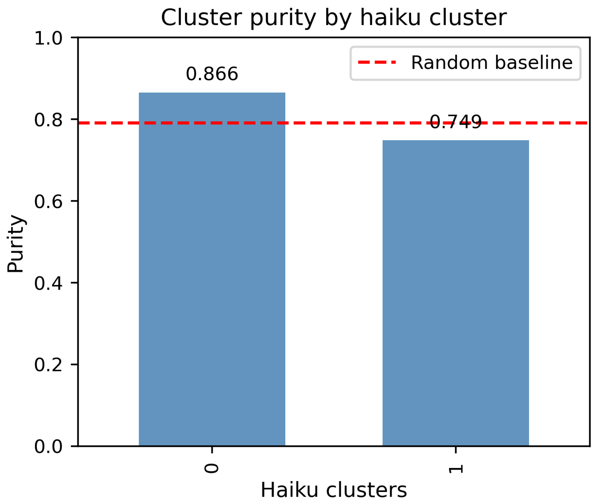
Cluster purity of haiku–music matches (Experiment D-2). Bars indicate the purity of each haiku cluster, defined as , and the dashed horizontal line shows the average purity under random shuffling of music-cluster labels. The observed average purity () is higher than the random baseline ().
Figure 23.
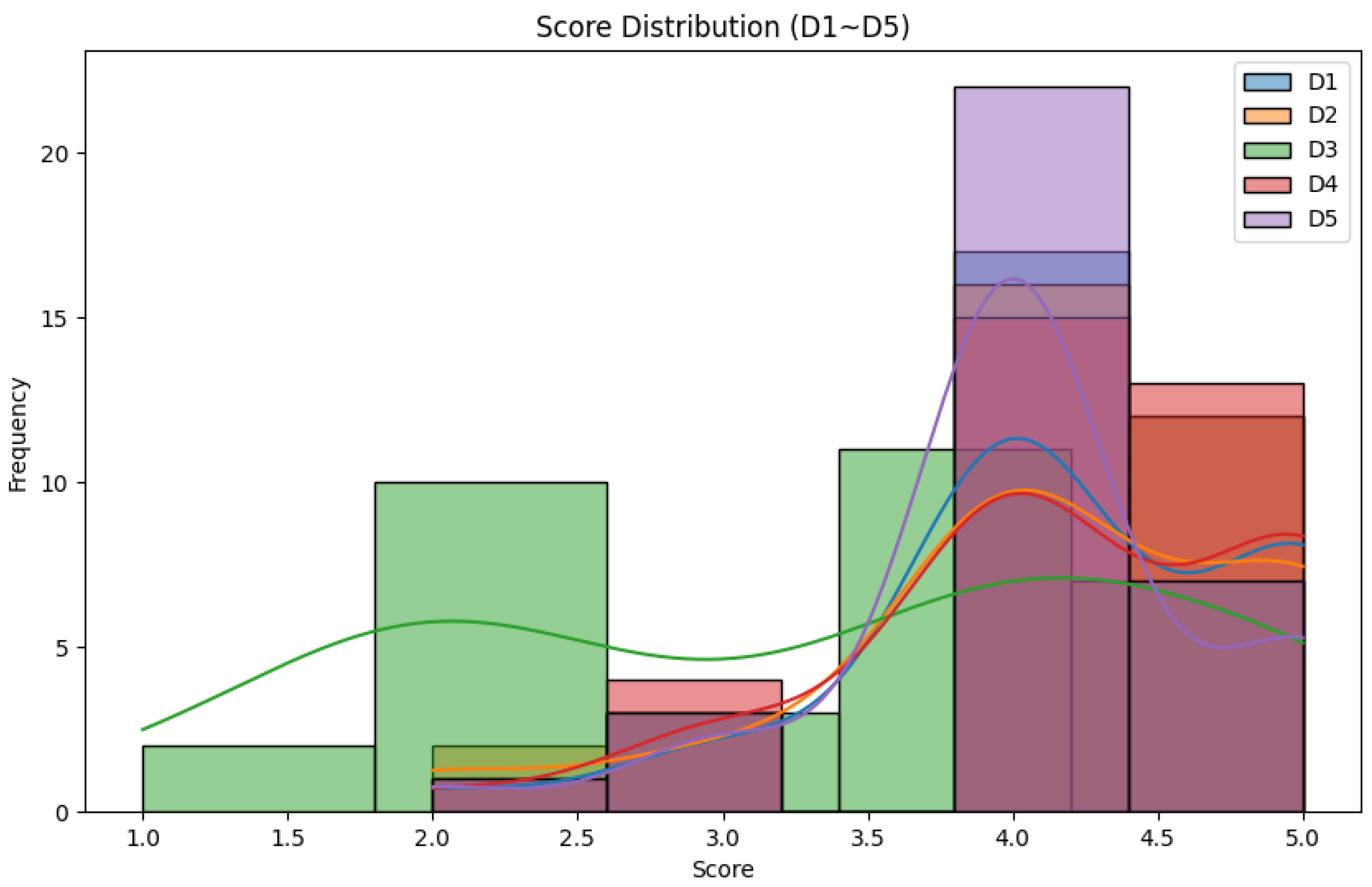
Score distribution for demonstrations (D1 to D5) is shown in the histograms and kernel density estimates. These show the distribution of participant ratings for each demonstration. Scores range from 1 (strongly disagree) to 5 (strongly agree).
Figure 23.
Score distribution for demonstrations (D1 to D5) is shown in the histograms and kernel density estimates. These show the distribution of participant ratings for each demonstration. Scores range from 1 (strongly disagree) to 5 (strongly agree).
Figure 24.
Mean and standard deviation of user ratings for the five demonstrations. Error bars indicate standard deviations.
Figure 24.
Mean and standard deviation of user ratings for the five demonstrations. Error bars indicate standard deviations.
Table 1.
Overview of the experiments conducted in this study, including their target modalities and evaluation objectives.
Table 1.
Overview of the experiments conducted in this study, including their target modalities and evaluation objectives.
| Exp. | Modality | Main Focus | What Is Evaluated |
|---|
| A | Text (haiku) | VED feature validity | Statistical stability, correlation structure, and seasonal consistency of BERT-based VED features, and whether they form an interpretable affective space for haiku. |
| B | Text (haiku) | Model comparison | TF-IDF, Word2Vec, and BERT as alternative text encoders; differences in cluster structure and seasonal trends; justification for adopting BERT as the baseline. |
| C | Music | Musical affective space (VET) | Construction and verification of Valence–Energy–Tempo features for Japanese-style instrumental tracks, and whether they yield coherent and discriminative emotional groups. |
| D | Cross-modal (text–music) | Affective alignment | Axis-wise correlations and cluster-level consistency between haiku VED and music VET, and whether a shared low-dimensional affective space supports haiku–music matching. |
| E | Multimodal + users | User perception | Participants’ ratings of haiku–image–music presentations, perceived coherence, unity, and usefulness of the multimodal appreciation interface. |
Table 2.
Basic statistics of normalized Valence, Energy, and Dynamism features.
Table 2.
Basic statistics of normalized Valence, Energy, and Dynamism features.
| Feature | Mean | Standard Deviation |
|---|
| Valence () | 0.49 | 0.18 |
| Energy () | 0.58 | 0.15 |
| Dynamism () | 0.50 | 0.19 |
Table 3.
Spearman correlation coefficients among normalized Valence, Energy, and Dynamism features.
Table 3.
Spearman correlation coefficients among normalized Valence, Energy, and Dynamism features.
| Feature | Valence () | Energy () | Dynamism () |
|---|
| Valence () | 1.00 | −0.86 | −0.71 |
| Energy () | −0.86 | 1.00 | 0.51 |
| Dynamism () | −0.71 | 0.51 | 1.00 |
Table 4.
Spearman correlations between normalized VED features and BERT principal components.
Table 4.
Spearman correlations between normalized VED features and BERT principal components.
| Feature | PC1 | PC2 | PC3 | PC4 | PC5 |
|---|
| Valence () | | | | | |
| Energy () | | | | | |
| Dynamism () | | | | | |
Table 5.
Kruskal–Wallis test results for seasonal differences in normalized Valence, Energy, and Dynamism features. p-values are rounded to two decimals; for Valence and Dynamism, , and for Energy, . Statistical significance is reported qualitatively using the descriptors “significant” () and “highly significant” ().
| Feature | Statistic (H) | p-Value | Significance |
|---|
| Valence () | 20.80 | 0.00 | Highly significant |
| Energy () | 11.36 | 0.04 | Significant |
| Dynamism () | 18.62 | 0.00 | Highly significant |
Table 6.
Cluster centers for Valence, Energy, and Dynamism features (standardized z-scores and normalized values).
Table 6.
Cluster centers for Valence, Energy, and Dynamism features (standardized z-scores and normalized values).
| Cluster | z-Score | Normalized [0,1] |
|---|
| | | | | |
| 0 (Calm/Positive) | 1.01 | | | 0.67 | 0.44 | 0.32 |
| 1 (Dramatic/Active) | | 0.53 | 0.55 | 0.39 | 0.66 | 0.61 |
Table 7.
Average silhouette coefficients for each encoder ( to 8).
Table 7.
Average silhouette coefficients for each encoder ( to 8).
| Model | k = 2 | k = 3 | k = 4 | k = 5 | k = 6 | k = 7 | k = 8 |
|---|
| TF-IDF | 0.60 | 0.53 | 0.49 | 0.49 | 0.50 | 0.50 | 0.51 |
| Word2Vec | 0.30 | 0.27 | 0.24 | 0.23 | 0.24 | 0.24 | 0.23 |
| BERT | 0.45 | 0.37 | 0.34 | 0.31 | 0.30 | 0.30 | 0.30 |
Table 8.
Axis-wise correlation between haiku (VED) and music (VET) features in Experiment D-1. Empirical correlations are contrasted with the randomly shuffled baseline.
Table 8.
Axis-wise correlation between haiku (VED) and music (VET) features in Experiment D-1. Empirical correlations are contrasted with the randomly shuffled baseline.
| Axis | Correlation r | 95% CI | Baseline Mean | Baseline SD |
|---|
| Valence | 0.971 | [0.968, 0.974] | 0.000 | 0.035 |
| Energy | 0.952 | [0.946, 0.957] | 0.003 | 0.030 |
| Dynamism/Tempo | 0.969 | [0.965, 0.973] | 0.001 | 0.034 |
Table 9.
Contingency matrix between haiku clusters () and music clusters () for the 1067 haiku–music pairs generated in Experiment D-1.
Table 9.
Contingency matrix between haiku clusters () and music clusters () for the 1067 haiku–music pairs generated in Experiment D-1.
| cluster_H | cluster_M = 0 | cluster_M = 1 | cluster_M = 2 |
|---|
| 0 | 335 | 2 | 50 |
| 1 | 509 | 170 | 1 |
Table 10.
Within-set CLIP similarity among ten generated images per haiku. Higher similarity values indicate greater reproducibility, while lower standard deviations reflect more stable generation behavior.
Table 10.
Within-set CLIP similarity among ten generated images per haiku. Higher similarity values indicate greater reproducibility, while lower standard deviations reflect more stable generation behavior.
| Haiku ID | Mean Similarity | Std. Deviation |
|---|
| 231 | 0.93 | 0.03 |
| 234 | 0.91 | 0.03 |
| 648 | 0.94 | 0.01 |
| 78 | 0.93 | 0.02 |
| 839 | 0.94 | 0.01 |
| 932 | 0.96 | 0.01 |


