Abstract
This study presents a comparative evaluation of state-of-the-art Machine Learning (ML) and Explainable Artificial Intelligence (XAI) methods, specifically SHAP and LIME, for predicting electromagnetic field (EMF) strength in urban environments. Using more than 19,000 in situ EMF measurements across Catalonia, Spain, combined with high-resolution geospatial features such as building height, built-up volume, and population density, six ML algorithms were trained and assessed over 50 randomized train–test splits. The k-Nearest Neighbors (kNN) model achieved the highest predictive accuracy (RMSE = 0.623), followed by XGBoost (RMSE = 0.711) and LightGBM (RMSE = 0.717). Explainability analysis showed that SHAP consistently identified built-up volume, building height, degree of urbanization, and population density as the dominant global predictors of EMF strength, whereas LIME revealed that degree of urbanization, population density, and building height were the most influential at the local (micro-scale) level. The results demonstrate that integrating interpretable ML frameworks with enriched geospatial datasets improves both predictive performance and transparency in EMF exposure modeling, supporting data-driven urban planning and public health assessment.
1. Introduction
The rapid proliferation of advanced technologies and their integration into nearly all aspects of personal, professional and industrial activity have transformed modern societies. Central to this transformation is the communication infrastructure, which has evolved to meet the increasing demands for high-speed, low-latency, and reliable connectivity [1,2]. Fifth-generation (5G) networks are now widely deployed, and the transition to sixth-generation (6G) technologies is already underway [3,4], enabling an unprecedented degree of interconnection among devices, systems, and users.
However, this technological expansion has led to the continuous and widespread exposure of human populations to electromagnetic fields (EMFs) [5,6] emitted by wireless communication systems. The dominant contribution arises from dense deployments of transmitting antennas, designed to meet growing coverage and capacity requirements [7]. Although international regulatory frameworks provide safety guidelines for exposure [8,9,10], the long-term health effects of chronic exposure to EMF remain an active area of scientific inquiry [11,12,13], fueling both societal concern and the need for rigorous monitoring [14,15,16,17].
In this context, two critical challenges emerge: first, ensuring that EMF levels remain within established safety thresholds to safeguard public health [18], and second, optimizing the distribution of transmitting antennas to simultaneously satisfy service quality and minimize population exposure [19,20]. Addressing these challenges requires an accurate prediction of EMF levels in heterogeneous urban environments [21,22,23], where variations in building density, topography, and user demand complicate the propagation patterns [24,25].
Traditional physics-based propagation models provide a partial solution, but are often limited by their simplifying assumptions and high computational cost when scaled to complex real-world environments [26]. Machine Learning (ML) methods [27,28,29], supported by Explainable Artificial Intelligence (XAI) frameworks [30,31], offer a promising alternative by enabling data-driven EMF prediction and also providing interpretability regarding the factors influencing model output. Such approaches not only enhance predictive accuracy, but also contribute to transparency in decision-making, a critical requirement for regulatory acceptance and public trust [32].
Although recent studies have improved EMF prediction using geospatial [33] and machine learning techniques [7,34], model interpretability remains insufficiently explored [35]. Prior work commonly applies SHAP [36], but rarely compares it directly with LIME for EMF strength prediction, and most analyses focus on a single urban area, limiting generalizability. This study addresses these gaps by systematically evaluating SHAP and LIME across multiple ML models and diverse urban environments. Overall, the aim is to compare state-of-the-art ML and XAI methods for EMF prediction while identifying the key spatial and environmental factors influencing EMF variability. By jointly analyzing SHAP (global explanations) and LIME (local explanations), this work provides a comprehensive and novel interpretability framework for EMF modeling, enhancing both predictive accuracy and understanding of EMF propagation in urban settings.
2. Related Work
In the era of rapidly advancing machine learning, numerous studies have been conducted within IoT frameworks to enhance prediction [37], automation, and intelligent environmental monitoring [27,38,39,40,41,42,43]. Research into electromagnetic field (EMF) strength is advancing rapidly, thanks to the integration of multidimensional datasets and cutting-edge methods like mathematical geospatial modeling, machine learning (ML), and explainable artificial intelligence (XAI). XAI, in particular, addresses the growing need to make scientific findings more interpretable [44]. These innovations greatly improve the depth and scope of research results.
2.1. Geospatial Methods for EMF and Environmental Monitoring
In a widely referenced practical study, Phillips et al. [45] explore the use of geostatistical methods for radio environment mapping (REM). They evaluated kriging and geostatistical techniques for mapping radio environments from sparse measurements, demonstrating that geostatistics offers accurate interpolation and explicit uncertainty estimates. The study also suggests hybrid GP/physics approaches for handling complex urban environments, making it a valuable resource for REM construction and sensor placement. Tesfay and Clavier [46] propose a Gaussian Process regression approach for EMF spatial reconstruction from sparse sensor data. The GP gives both mean field estimates and spatial uncertainty; with an informative mean and properly chosen kernel it outperforms zero-mean GP and naive interpolation in their experiments. The study stresses the usefulness of GP uncertainty maps to guide sensor placement.
In a more complex approach as part of consecutive novel studies, Kiouvrekis et al. [47] evaluated five geospatial modeling methods to create national-level EMF exposure maps, using 3621 measurements over a 9251 km2 area. Gaussian Process Regression models, also known as Kriging models, outperformed others in accuracy; however, when outliers were removed, the classical nearest neighbor method showed comparable performance. In general, the study highlights the importance of model selection and data quality in accurately assessing EMF exposure for public health considerations. In a relevant study, Panagiotakopoulos et al. [48] investigated geospatial interpolation modeling techniques of electromagnetic field (EMF) exposure by also using Gaussian Process Regression (Kriging) and nearest-neighbor interpolation for large-scale EMF mapping. Using an enriched feature dataset of 3632 measurements collected in Paris, their study demonstrated that Kriging, particularly with the exponential covariance model, achieved superior predictive accuracy by effectively capturing spatial autocorrelation in the EMF data, while outlier removal further improved model performance by reducing both mean square error (MSE) and variability.
Jorge Guillen-Pina et al. [24] in their study presented an innovative multi-method ensemble algorithm for optimization (PCRO-SL) to create EMF exposure maps using multi-method evolutionary ensembles, specifically genetic algorithms, to optimize measurement point selection. This approach allows for efficient exploration of the solution space to identify optimal configurations of measurement points and so significantly reduces the number of required measurements while maintaining the accuracy of the map, offering a resource-efficient solution for urban EMF monitoring.
2.2. ML Models Used in EMF Prediction and Environmental Monitoring
Artificial Intelligence, through innovative Machine Learning techniques, seeks to enhance the accuracy, adaptability, and efficiency of well-established mathematical geospatial methods in EMF predictions. In this spirit, Yarui Zhang et al. [28] proposed ExposNet, a deep learning framework that predicts the levels of the electric field in urban environments using real-world measurements and data from the base station. By encoding environmental features as multidimensional tensors for input to CNNs, the model captures complex spatial patterns and achieves improved prediction accuracy, demonstrating the potential of deep learning in environmental monitoring. In another study, Xinwei Song et al. [49] compared six predictive models for forecasting RF-EMF exposure in urban settings using two years of monitoring data from Novi Sad, Serbia. Among the models evaluated, PLS, CNN and Transformer models outperforming the others but with the Partial Least Squares Regression (PLS) demonstrated superior accuracy and efficiency above all, suggesting its suitability for real-time EMF exposure monitoring and public health protection initiatives.
Wang and Wiart [50] developed a hybrid artificial neural network model designed to efficiently process various input data, including spatial and temporal variations in exposure to EMF to map urban exposure to EMF by integrating sensor data, drive tests and public BSA information. Applied to Paris’s 14th district, the model outperformed traditional methods, effectively capturing complex spatial variations in EMF exposure. The study offers a cost-effective and accurate approach to urban EMF monitoring. Mallik et al. [51] proposed a generative method, GLIP (Generative Local Image Prior), to reconstruct electromagnetic field (EMF) exposure maps from sparse sensor data. Instead of training a full GAN, GLIP employs a pretrained generator as an image prior, optimizing its latent space to match sparse measurements while preserving realistic spatial structures. Evaluated on simulated and real EMF datasets, GLIP outperformed traditional interpolation techniques (e.g., Kriging, nearest-neighbor) in accuracy and spatial coherence, demonstrating its effectiveness in data-sparse EMF mapping scenarios.
Bilson et al. [52] proposed a physics-informed machine learning (PIML) framework to model RF-EMF exposure from 5G massive multiple-input-multiple-output (mMIMO) base stations. By integrating wave propagation physics and antenna radiation patterns into neural network training through physics-based loss terms, the approach enforces physically consistent predictions and improves extrapolation in sparse data regions. Evaluations in simulated and real scenarios show that the PIML model achieves lower RMSE and greater robustness than purely data-driven or physics-only methods, offering an efficient and physically grounded solution for large-scale EMF mapping. Shahid et al. [53] proposed ReVeal, a physics-informed neural network (PINN) for radio environment mapping (REM) that embeds a path-loss PDE into the learning objective to enforce physical consistency while fitting sparse RF measurements. By combining data-driven learning with propagation constraints, ReVeal achieves high-fidelity RSS maps with improved RMSE, robustness, and data efficiency compared to standard ML and classical models. Evaluations of real-world ARA testbed data demonstrate substantial accuracy gains and reduced sample requirements, highlighting ReVeal’s suitability for large-scale and resource-constrained EMF mapping.
2.3. Use of XAI in Spatial and Environmental Predictions
Although the wide application of machine learning techniques in the prediction of EMF and the implementation of environmental research has achieved remarkable results, the need for interpretability and comprehensive, human-understandable documentation of the results has become more evident than ever. In this spirit, the study of Abekoon et al. [54] developed a deep neural network (DNN) to predict soil nitrogen (N), phosphorus (P) and potassium (K) levels in cabbage cultivation based on plant growth metrics such as height, leaf count and leaf area. The study was applied over an 85-day period in Sri Lanka’s central highlands, with the model aimed to support soil fertility assessment without extensive chemical tests. To improve transparency and interpretability, the study used explainable AI (XAI) techniques, namely SHAP and LIME, offering clear insights into the contribution of the features and enhancing the relevance of the model for precision agriculture and sustainable soil management. Junhao Zhang’s study [55] applies the LightGBM model to predict water potability using various water quality indicators. To interpret the model’s predictions, the research compares SHAP and LIME techniques. SHAP offers a global view, identifying sulfate and pH as key features, while LIME provides local explanations for individual predictions through a local linear approximation. The study concludes that SHAP is suitable for understanding the overall behavior of the model, whereas LIME is more effective for interpreting specific instances.
Kiouvrekis et al. [36] developed an explainable machine learning framework to map the strength of the electric field in Paris using an enriched dataset incorporating geographical features such as building volume and population density. Among 410 models evaluated, the k-nearest neighbors (kNN) algorithm demonstrated the most consistent performance, generating the lowest RMSE and standard deviation. To improve interpretability, SHapley Additive exPlanations (SHAP) were applied, revealing that the building volume around each antenna was the most influential predictor of EMF levels, followed by population density. The resulting dynamic maps offer valuable insights for urban planning and public health. Xianlin Ma et al. [56] developed interpretable machine learning models to predict tight gas well productivity using data from the Eastern Sulige field in China. They developed machine learning models, including Support Vector Machines (SVMs), Gradient Boosting Decision Trees (GBDTs), and Random Forest (RF), to forecast well productivity. Among these, the GBDT model demonstrated the most superior predictive performance. By applying SHAP and LIME, the study provided global and local explanations of model predictions, enhancing the understanding of key factors that affect productivity and helping in strategic decision-making. Nasir and Li [57] applied advanced machine learning models such as ANN, GBM, RF, XGBoost, and a hybrid RF-GBM, to predict key wastewater treatment plant (WWTP) variables such as BOD, TSS, , and P using multi-year operational data. To enhance interpretability, SHAP and LIME were employed, revealing the most influential features driving the model predictions. The results demonstrated high predictive accuracy and strong generalization, while the integration of XAI improved transparency and informed data-driven optimization of WWTP operations.
In another novel study, Kiouvrekis et al. [31] evaluated 566 machine learning models to predict electric field strength in eight French cities by integrating sensor-based EMF data with urban features such as population density, urbanization, and building characteristics. Among the six machine learning approaches tested, the ensemble methods, in particular Random Forest and XGBoost, achieved the highest predictive accuracy, especially when including geographic features as predictive variables. To enhance interpretability, SHAP was employed to interpret model outputs, revealing notable differences in feature importance rankings between tree-based and other machine learning models. A study by Kalatzis et al. [30], which conducted in Cyprus applied Explainable Artificial Intelligence (XAI) techniques to analyze electromagnetic field (EMF) exposure across multiple frequency bands (30 MHz–6 GHz) from mobile, radio, and television sources. Six machine learning models were compared, with ensemble methods, particularly Random Forests and LightGBM, achieving the highest predictive accuracy. Using SHAP, the study identified key spatial and demographic factors influencing EMF intensity, supporting transparent, data-driven exposure mapping for urban planning and public health assessment.
However, despite the significant progress demonstrated in the reviewed studies, several limitations remain evident in the current body of research. Most existing work has focused on improving predictive accuracy through advanced machine learning or on enhancing spatial interpolation via geospatial models, yet few have systematically addressed the interpretability of EMF prediction models. Although SHAP has been increasingly adopted for global explainability, there is a notable absence of studies that directly compare SHAP and LIME in the context of EMF strength prediction, particularly when combined with heterogeneous geospatial and environmental datasets. Furthermore, existing explainable approaches often concentrate on a single urban area or frequency band, limiting the generalizability and scalability of their findings across diverse urban morphologies. To bridge these gaps, the present study aims to provide a comprehensive comparative analysis of SHAP and LIME applied to multiple machine learning models for the prediction of the strength of EMF in several urban and semi-urban areas, collected using a hybrid system of fixed and portable measuring instruments. So, by coupling rigorous geospatial feature engineering with extensive evaluation of ML models and interpretable AI techniques, this work seeks to advance both the transparency and the scientific reliability of EMF exposure modeling in complex urban environments.
3. Materials and Methods
3.1. The Dataset
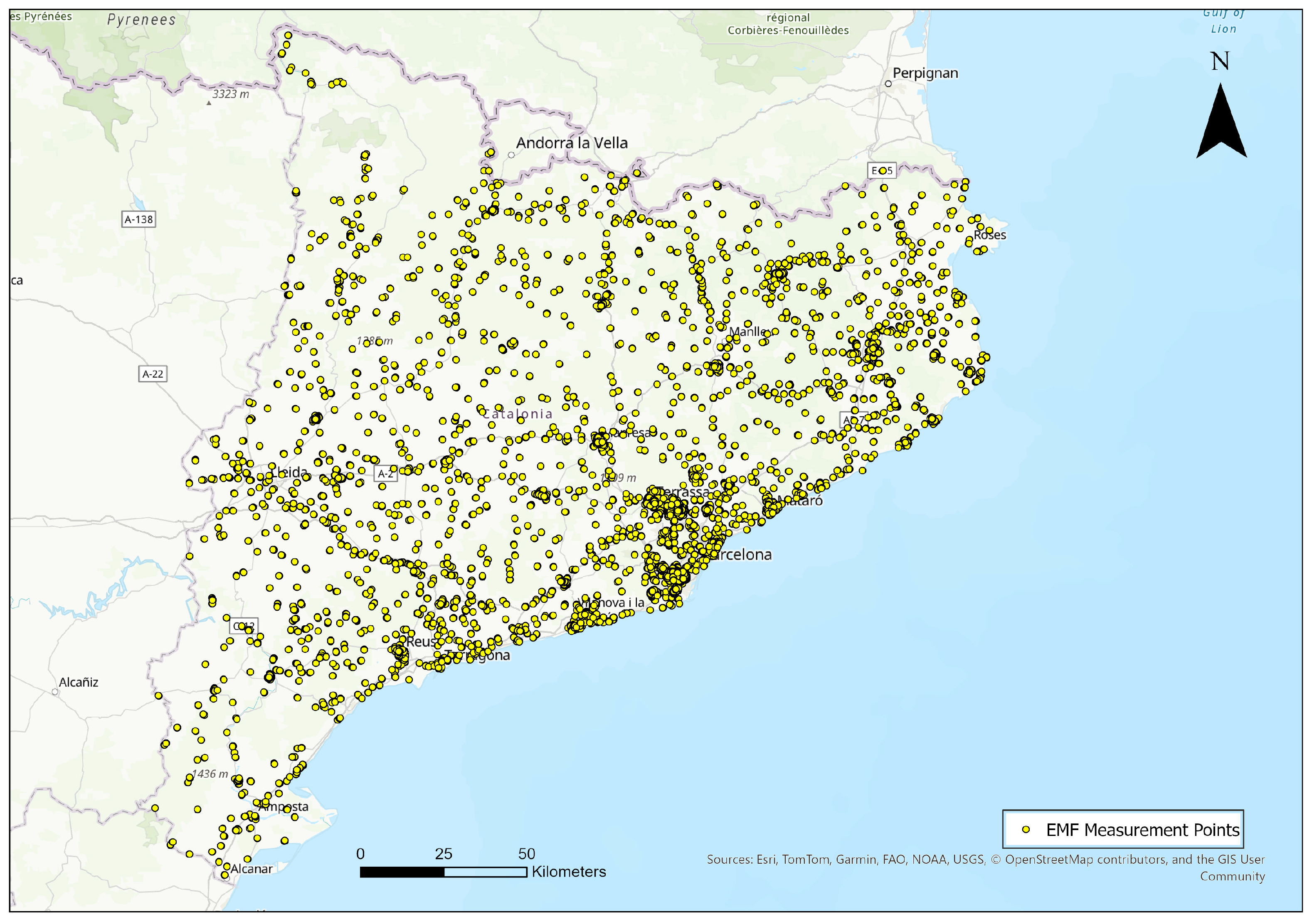
The data set [58] used in this study originates from the official open data platform of the Spanish Government, which provides measurements of radio-frequency electromagnetic field (EMF) exposure collected through certified monitoring campaigns. During the period 2013–2015, within the framework of the Governança Radioelèctrica project [59], a comprehensive electromagnetic field (EMF) measurement program was carried out in Catalonia. For this purpose, a combined system of fixed and portable measuring instruments was used, allowing continuous monitoring and recording on-site in sensitive areas such as schools and hospitals (Figure 1). A total of 100 fixed monitoring stations were installed on roofs of buildings with a direct line-of-sight to the antennas. Ninety of them operated on photovoltaic power, while ten operated as electrically powered units. These stations measured either specific mobile telephony frequency bands (900, 1800, 2100 MHz) or the full spectrum from 100 kHz to 8 GHz. In parallel, 50 portable devices were distributed to municipalities and public bodies, enabling more than 19,322 measurements at 4598 locations.
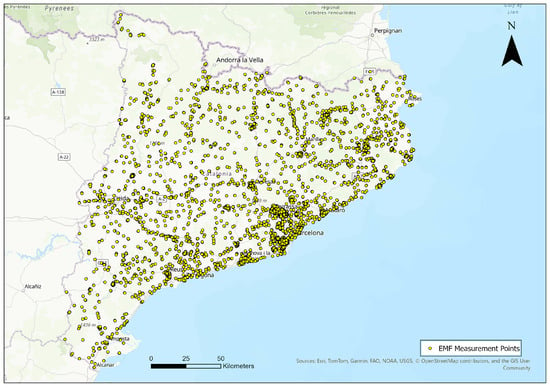
Figure 1.
Spatial distribution of EMF (Electromagnetic Field) measurement points across Catalonia, Spain.
Each record in the dataset corresponds to a specific measurement report, containing details such as location, date of assessment, measurement type and the recorded average field strength. The data set covers a wide geographic coverage in various municipalities and administrative regions, reflecting real-world environmental EMF conditions. Measurements are typically conducted using portable spectrum analyzers or fixed monitoring equipment, following standardized protocols to ensure reliability and comparability.
The variables used in this study were derived from the Global Human Settlement Layer (GHSL) Data Package 2023 (GHS P2023) developed by the European Commission’s Joint Research Centre (JRC, 2024). These datasets provide globally consistent, open-access spatial information describing the built environment, population distribution, and settlement structure from 1975 to 2030. All datasets were resampled and aligned to a common grid of 100 m spatial resolution with geographic coordinates corresponding to longitude and latitude of the grid cell centroid (see Table 1).

Table 1.
Summary of GHSL datasets used in the study, including variable type, spatial resolution, temporal coverage, and coordinate reference.
The GHS-BUILT-S R2023A variable represents the fraction of built-up area within each grid cell, derived from Sentinel-2 and Landsat imagery for epochs between 1975 and 2030 (5-year intervals). It provides sub-pixel built-up estimates at 10 m and aggregated 100 m resolution, distinguishing between residential (RES) and non-residential (NRES) domains. This layer serves as a measure of horizontal urban expansion and built-up density. The GHS-BUILT-H R2023A variable provides average building height (in metres) for each 100 m grid cell, estimated from the integration of AW3D30, SRTM30, and Sentinel-2 data (epoch 2018). It captures the vertical dimension of the built environment, enabling analyses of urban morphology and 3D structural variation. The GHS-BUILT-V R2023A variable combines the built-up surface and height layers to estimate built-up volume (m3/cell) for 1975–2030 at 100 m resolution. It expresses the volumetric density of constructed space, reflecting the total built infrastructure per unit area. This is a critical indicator of the intensity of urban development and infrastructure stock. The GHS-BUILT-C R2023A variable integrates built-up surface, height, and population layers to describe settlement characteristics and urban form. It includes metrics of built-up density, morphology, and functional classification at 10–100 m resolution for 2018. This variable enables the identification of heterogeneous settlement typologies and spatial organization patterns. The GHS_BUILT_C_MSZ layer classifies morphological settlement zones (MSZ) based on built-up density and spatial configuration, distinguishing continuous urban fabric, suburban, and rural morphologies. It provides categorical information useful for urban form classification and sprawl analysis. The GHS-POP R2023A variable provides multi-temporal population density grids (inhabitants per cell) for 1975–2030 in 5-year intervals at 100 m and 1 km resolutions. Population counts are derived by downscaling national and subnational census data using residential built-up volume (RES) as a weighting layer, aligned to the UN World Population Prospects (2022) and World Urbanization Prospects (2018). The GHS-SMOD R2023Avariable classifies the Earth’s surface into urban centres, dense urban clusters, and rural grid cells following the Degree of Urbanisation (DEGURBA) Stage I methodology. It integrates GHS-BUILT-S and GHS-POP data to describe the spatial hierarchy of settlement systems between 1975 and 2030.
3.2. Framework for Machine Learning and Explainable AI
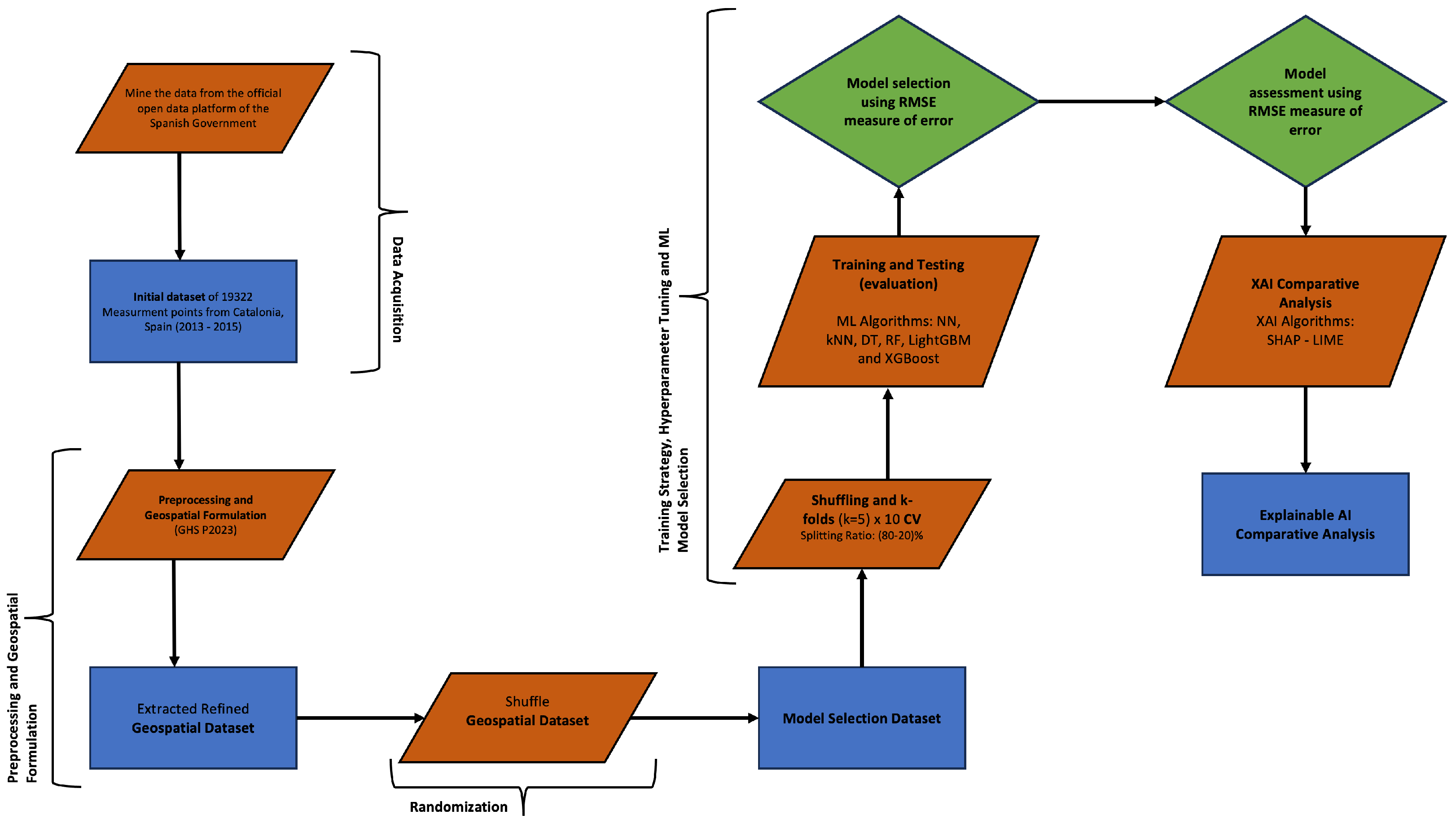
This study follows a structured, reproducible workflow designed to ensure robust electromagnetic field (EMF) prediction and model interpretability, integrating geospatial preprocessing, systematic ML benchmarking, and dual XAI evaluation (Figure 2). The workflow begins with raw EMF measurements from the official Spanish governmental open-data platform, followed by comprehensive quality control including missing-value handling, physical-plausibility checks, distributional inspection, and robust outlier filtering techniques. All geospatial variables are formalized and enriched with refined urban-morphology attributes from the GHSL Data Package 2023, producing a unified spatial dataset suitable for ML experimentation.

Figure 2.
Machine Learning—XAI pipeline.
A randomized shuffling stage ensures independence in sampling order prior to model training. To mitigate spatial autocorrelation biases, we employ 50 stratified train–test splits (80/20) with unique seeds, verifying no leakage and maintained target-variable representativeness across splits. This repeated partitioning strategy provides a low-variance generalization estimate and robust cross-validation. Six ML models were then benchmarked, Neural Networks, k-Nearest Neighbors, Decision Trees, Random Forests, LightGBM, and XGBoost, each trained over a structured hyperparameter grid and evaluated via mean RMSE, standard deviation, and 95% confidence intervals across all folds. Best configurations were subsequently retrained and independently assessed to confirm generalization.
Model interpretability was conducted on the top-performing models using SHAP and LIME. SHAP provided global feature attribution and instance-level decomposition, while LIME offered localized surrogate explanations aggregated across samples. This dual-lens analysis enabled assessment of both global explanatory stability and local contextual behavior. Together, the pipeline workflow delivers a transparent, rigorously validated, and scientifically accountable framework for EMF estimation in urban environments, ensuring methodological robustness, reproducibility, and interpretability.
3.3. Description of Machine Learning Methods
Machine learning (ML), a core branch of artificial intelligence, facilitates data-driven modeling by identifying patterns and generating predictions with minimal human intervention. In this study, ML techniques are employed to accurately predict and map electromagnetic field (EMF) strength in urban environments, integrating spatial and structural features to enhance environmental monitoring. Before detailing the specific algorithms, architectures, and hyperparameters, it is important to highlight two fundamental hyperparameters common across most ML models: the learning rate and the optimizer. The learning rate governs the magnitude of parameter updates during optimization, directly influencing model convergence and stability, while the optimizer determines the update strategy for minimizing the loss function. Proper selection or tuning of these parameters is essential to balance convergence speed, accuracy, and generalization across different ML methods.
Neural Networks (NN) Neural Networks (NNs) are computational models inspired by biological neural systems, composed of interconnected neurons organized into input, hidden, and output layers. Each neuron processes weighted inputs and biases through nonlinear activation functions (e.g., ReLU, sigmoid, tanh), enabling the network to approximate complex nonlinear mappings. The network’s depth, determined by the hyperparameter that controls the number of hidden layers , which define the total depth of the NN and directly influences its representational capacity but also affects overfitting risk. Training is performed via backpropagation using gradient descent-based optimization to minimize a loss function, such as Mean Squared Error for regression or Cross-Entropy for classification. In this study, a set of neural network models were employed, with hyperparameter tuning over the number of hidden layers , activation functions , and learning rates , while the Adam optimizer was used and all the other hyperparameters kept at default settings.
k-Nearest Neighbors (k-NN)
The k-Nearest Neighbors (k-NN) algorithm is a non-parametric supervised learning method used for classification and regression, based on the principle that similar data points in the feature space exhibit similar outcomes. For a query point x, the algorithm identifies the k nearest samples and predicts the output as either the majority class (classification) or the mean/weighted mean of neighboring target values (regression). Model performance depends primarily on the choice of k, the distance metric, and the weighting scheme. Distance can be computed using various norms—Euclidean , Manhattan , or Minkowski—while weights may be uniform or distance-dependent, e.g., inverse distance or Gaussian . In this study, three hyperparameters were optimized: the number of neighbors , distance metric parameter , and weighting scheme (uniform vs. distance-based).
Decision Trees (DTs)
Decision Trees (DTs) are nonparametric supervised learning models applicable to both classification and regression tasks. They recursively partition the feature space through hierarchical, feature-based splits to form a tree structure of decision and terminal nodes. Splits are chosen to maximize node purity using criteria such as Gini Impurity or Entropy , with information gain guiding the optimal partitioning. For regression, variance reduction serves as the splitting criterion. In this study, a minimal configuration was adopted to establish a baseline for comparison with ensemble tree models, varying only the hyperparameter controlling the minimum samples required to split a node within .
Random Forest (RF)
Random Forest (RF) is an ensemble learning algorithm that enhances predictive accuracy and generalization for both classification and regression by aggregating multiple Decision Trees trained on bootstrap samples (bagging) and random feature subsets. This dual randomness reduces inter-tree correlation and mitigates overfitting. The final prediction is obtained via majority voting (classification) or averaging (regression). Feature importance is derived from the mean impurity reduction across all trees, quantifying each variable’s contribution to model performance. In this study, the Random Forest was tuned by varying the number of trees , the splitting criterion , and fixing the maximum tree depth to 10.
LightGBM
Light Gradient Boosting Machine (LightGBM) is an efficient ensemble algorithm based on Gradient Boosting Decision Trees (GBDTs), optimized for speed and scalability. Unlike traditional level-wise boosting, LightGBM adopts a leaf-wise growth strategy, expanding the leaf with the greatest loss reduction to enhance accuracy while preserving efficiency through histogram-based feature binning. Each tree minimizes a differentiable loss function by fitting the residuals of prior predictions, updating the model as
where is the tree added at iteration t and is the learning rate. In this study, four key hyperparameters were tuned: the number of leaves , number of trees , maximum depth , and learning rate , balancing model complexity, convergence speed, and generalization performance.
XGBoost (Extreme Gradient Boosting)
Extreme Gradient Boosting (XGBoost) is an optimized implementation of the gradient boosting framework that constructs decision trees sequentially, with each tree correcting the residuals of its predecessors. It minimizes a regularized objective function,
where denotes the loss and penalizes model complexity, thereby enhancing generalization. Optimization is guided by first- and second-order gradients, enabling precise and efficient updates. XGBoost incorporates regularization, sparsity-aware learning, and parallelized computation, achieving both scalability and robustness.
For this study, the tuned hyperparameters were the L2 regularization term , the number of trees , the maximum tree depth (fixed at 20), and the learning rate , ensuring an optimal balance between bias, variance, and computational efficiency.
The Table 2 above summarizes the hyperparameter configurations explored for each machine learning model. The selected ranges were designed to systematically probe the trade-off between model complexity, generalization capacity, and computational efficiency, ensuring a balanced and reproducible experimental framework. For Neural Networks (NN), variations in the number of hidden layers, activation functions, and learning rates capture the effect of network depth and nonlinear activation on convergence and overfitting control. In k-Nearest Neighbors (k-NN), tuning the number of neighbors, distance metric, and weighting scheme examines the locality dependencies of the feature space and the influence of metric geometry on model’s performance. For Decision Trees (DTs), the minimum samples per split parameter isolates the relationship between node purity and model variance, while keeping DTs as a simple, interpretable baseline for ensemble comparison. Random Forest (RF) tuning included ensemble size and splitting criterion, maintaining fixed depth to evaluate ensemble effects independently of tree complexity. In LightGBM, the number of leaves, boosting iterations, maximum depth, and learning rate were adjusted to control tree growth, regularization strength, and learning dynamics. Similarly, for XGBoost, tuning the L2 regularization term , number of trees, maximum depth, and learning rate allowed examination of the algorithm’s balance between model expressiveness, regularization, and convergence speed. The chosen hyperparameter combinations were designed to cover a range of low-to-high capacity levels across algorithms, enabling a thorough comparison of bias-variance behavior, stability, and computational cost, all within a consistent cross-validation framework.

Table 2.
Machine Learning Models Hyperparameters Configurations.
A Grid Search Approach
In this study, hyperparameter tuning was performed by using Grid Search, a systematic and exhaustive optimization technique that evaluates all possible combinations within a predefined discrete hyperparameter space in order to identify the configuration yielding the optimal model performance. Formally, Grid Search seeks the combination , where is the cartesian product of the hyperparameter space and represents the objective function, here defined as the mean RMSE obtained through cross-validation. Although computationally intensive due to its combinatorial nature, this approach ensures a thorough exploration of the hyperparameter space, providing a deterministic and reproducible framework for model selection and establishing a robust baseline for performance optimization. Additionally, it’s worth noting that, for the purposes of this study, we predefined the hyperparameter values based on other relevant and valid studies in the field [11,27,30,31,36,47]. This decision was made to address the exponential nature of grid search concerning the number of hyperparameters and to prevent potential computational infeasibility of the machine learning models.
3.4. Metrics-Accuracy Evaluation
To ensure the effective deployment of electromagnetic field (EMF) prediction models and exposure maps, it is crucial to establish robust measures of predictive reliability. Among the various error metrics used to evaluate model performance, the Root Mean Squared Error (RMSE) is one of the most widely employed in regression analysis and machine learning tasks. RMSE quantifies the square root of the average squared differences between predicted and observed values, providing an interpretable and sensitive indicator of overall model accuracy. Formally, it is defined as:
where denotes the true value, the predicted value, and n the total number of observations. The squaring of the errors emphasizes larger deviations more than smaller ones, making RMSE particularly sensitive to outliers. As such, it serves as a comprehensive measure of model performance by combining both the variance and bias of the estimator into a single value expressed in the same units as the dependent variable. A lower RMSE indicates better model performance, with predictions closely aligned to actual values. However, the sensitivity of RMSE to large errors implies that it may not always be the best choice when robustness to outliers is required, a feature which must be taken under consideration during the design of the model.
3.5. Explainable AI Methods
Results without explanations, without reasoning, is just mechanistical stripped computations. As machine learning models become increasingly complex, often involving sophisticated mathematical formulations, their interpretability correspondingly diminishes. Moreover, with the growing integration of artificial intelligence (AI) and machine learning (ML) across a wide range of critical domains, the demand for transparent and interpretable models has become paramount. In response to this challenge, various explainable AI (XAI) techniques have been developed, among which SHAP (SHapley Additive exPlanations) and LIME (Local Interpretable Model-agnostic Explanations) are prominent, offering systematic approaches to elucidate model behavior and foster trust in model predictions.
Broadly speaking, in mathematics and formal sciences, a model refers to a mathematical structure used to interpret the symbols and formulas of a formal language or to represent a class of phenomena. Specifically, in the context of machine learning (ML), a model is a parameterized mathematical function (or family of functions) trained to approximate a relationship between inputs and outputs. Formally, given:
- an input space ,
- an output space and
- training data .
Then a model is a function parameterized by (where is a parameter space). The goal is to find parameters such that “best fits” the data according to some loss function , usually by solving an optimization problem like:
Thus, the model is a hypothesis in a hypothesis space .
Consider, for example, a linearly separable Support Vector Machine (SVM) problem with input and parameters , . The general model for the class of linear SVMs can be expressed as:
For each distinct set of parameters , a different model is obtained, along with a corresponding partition of the data. This partition is determined by the hyperplane that separates the classes with the maximum margin. The objective is to identify the optimal hyperplane that maximizes the margin between the classes, typically by minimizing an error metric or a loss function designed to achieve this goal. So, by realizing the inherent enormous complexity that machine learning models can have, the need to develop models with sufficient explainability of the results (valuations of the models) is imperative.
3.5.1. SHAP
SHapley Additive exPlanations (SHAP) is a unified framework for interpreting machine learning model predictions based on cooperative game theory. It leverages the concept of Shapley Values to attribute the output of a model to its input features fairly and consistently. In this framework, each feature is treated as a “player” in a coalition, and the model’s output is considered the “payout” that the players collectively generate. The Shapley value for a given feature represents its average marginal contribution to the prediction across all possible subsets of features.
The practical implementation of SHAP enables both global and local interpretability. Locally, SHAP values explain individual predictions by quantifying the positive or negative contribution of each feature relative to a baseline expectation (typically the mean model output). Globally, aggregating SHAP values across a dataset highlights the overall importance and influence of features on model behavior. Our approach employs a specific type of explanation model that aggregates the contributions of additive feature attribution methods, where the explanation model is represented as a linear function mathematically expressed such as:
where denotes binary variables, n denotes the number of simplified input features, and denotes the attribute effect. The SHAP value for a feature i is defined as:
where N denotes the set of all features, S is a subset of features not containing i, is the model output when only features in S are present, and is the output when feature i is added to S. The above expression captures the average marginal contribution of feature i over all possible subsets S, ensuring fairness in attribution, by satisfying properties such as:
- Local Accuracy: When the transformation is identified with x, then the explanation model matches the original model, i.e., .
- Missingness: Simply, if , then . This means that this feature has no attributable impact when . Missingness implies that a missing feature receives an attribution of zero.
- Consistency: The attribution values remain unchanged unless there is a variation in a feature’s contribution to the prediction. More critically, the consistency property ensures that if a feature’s influence on the model’s output increases, its corresponding Shapley value must either increase or remain constant.
SHAP offers an additive explanation model in which the prediction is decomposed into a sum of contributions from each feature, thereby enhancing transparency and trust in complex predictive systems.
However, the exact computation of SHAP values is computationally expensive, as it requires evaluating the model on all subsets of features, which becomes infeasible for large M. To mitigate this challenge, SHAP leverages approximation methods such as Kernel SHAP, Tree SHAP, and Deep SHAP, each offering either a model-agnostic or model-specific approach, depending on the computational context. These methods reduce the computational complexity from exponential to polynomial time, making SHAP a practical and scalable tool for interpreting complex models in real-world applications.
3.5.2. LIME
Local Interpretable Model-agnostic Explanations (LIME) is another widely adopted method within the domain of explainable artificial intelligence (XAI) that aims to provide interpretable explanations for individual predictions of complex machine learning models. It operates under the principle that complex models can be locally approximated by simpler, interpretable models. So, as a model-agnostic technique, LIME is designed to be applicable across a broad range of classifiers and regressors without requiring access to the internal structure of the model. Its primary objective is to generate locally faithful approximations of a model’s behavior in the vicinity of a specific instance by constructing an interpretable surrogate model, typically a sparse linear regression model.
Specifically, given a black-box model and an instance , LIME seeks to approximate f in the vicinity of x using an interpretable model , where G is a class of simple models (e.g., linear models, decision trees). The objective is to minimize the following loss function:
where:
- measures the fidelity of g in approximating f in the locality defined by .
- is a proximity measure between the instance z and the instance x, often defined as an exponential kernel:
- is a distance metric (e.g., Euclidean distance), and controls the width of the neighborhood.
- is a complexity penalty to ensure interpretability, such as the number of non-zero coefficients in a linear model.
- The loss function is typically the weighted squared loss:where Z is a set of perturbed samples around x.
The overall methodology involves perturbing the input instance to create a set of synthetic samples and evaluating these samples using the original black-box model to obtain predicted outcomes. In particular, it incorporates the following algorithmic steps:
- Data Perturbation: Generate a dataset Z of perturbed samples around the instance x.
- Prediction: Obtain the black-box model’s predictions for each perturbed sample .
- Weighting: Compute the proximity for each z to weigh the importance of each sample in the local approximation.
- Interpretable Model Training: Fit the interpretable model g on the dataset Z with weights , minimizing the loss while considering the complexity penalty .
- Explanation: Present the interpretable model g as the explanation for the prediction . For linear models, the coefficients indicate the contribution of each feature.
LIME’s focus on local fidelity ensures that the explanations accurately reflect the model’s behavior in the immediate region surrounding the prediction, thereby enhancing transparency and user trust. Moreover, its model-agnostic nature and intuitive output make LIME a versatile and effective tool for interpreting the decisions of complex machine learning systems in a wide array of application domains.
4. Results
4.1. Machine Learning Model Selection Results
This section presents a comprehensive analysis of the results obtained from the systematic application of the machine learning methods described previously. For each method, hyperparameter optimization yielded a distinct set of models, enabling a thorough evaluation of their performance. We provide a detailed discussion of the optimal results for each algorithm individually, followed by a comparative analysis to assess their relative performance and effectiveness.
To provide additional practical value, we report the computational burden associated with the hyperparameter grid and model training process. Across all experiments, the relative runtime order was as follows: kNN was the fastest method, followed by Decision Trees, which also completed training quickly. XGBoost and LightGBM required moderate computation time, while Neural Networks exhibited moderate to high runtime depending on the number of layers and complexity of the architecture. Random Forest showed the highest overall computational cost due to the large number of trees and repeated cross-validation. These observations help practitioners understand the trade-off between predictive accuracy and computational resources when selecting models for large-scale EMF prediction tasks.
Neural Networks (NN)
We implemented a large-scale evaluation of neural network architectures, systematically varying hyperparameters related to topology (number of layers L), activation functions (), and optimization settings (learning rate , optimizer choice). The best-performing configurations achieved mean RMSE values between 0.909277 and 0.911257, with differences lying within the error margin, indicating comparable accuracy and robustness across cross-validation folds. The numerical optimal model consisted of two hidden layers with ReLU activation, Adam optimizer, and , yielding a mean RMSE of 0.909277 (). Although ReLU combined with high learning rates produced competitive results, these models exhibited lower reproducibility.
In contrast, networks with logistic or tanh activation functions, compact architectures (2–20 hidden units), and moderate learning rates (, Adam) consistently achieved near-optimal accuracy while maintaining greater stability. These models dominated the top-ranked results, underscoring their reliability and efficiency in capturing nonlinear patterns in electric field strength prediction, as we can see in the summarized ranking Table 3. Conversely, identity activations and excessively large networks often diverged, producing inflated errors and instability, highlighting their unsuitability. Overall, compact architectures with logistic or tanh activations and moderate learning rates represent the most robust and practical solutions for deployment, while further statistical paired tests on fold-level predictions are required to claim that any of the best configurations is better than another.

Table 3.
Top 10 Neural Network Hyperparameter Combinations Ranked by Mean RMSE.
k-Nearest Neighbors (kNN)
The evaluation of the k-Nearest Neighbors (kNN) models revealed a consistent trend of better results by the use of distance-based weighting schemes (inverse-distance) over uniform weighting (equal weights), regardless of the number of neighbors or Minkowski distance parameter p. Specifically, the five best-performing configurations, as measured by mean RMSE, were very tightly grouped in the interval [0.623153, 0.627706], with the best of them achieving RMSE 0.623153 (SD 0.042993), closely followed by the second best with RMSE 0.623335 (SD 0.043059), and the rest of the top 5 as clearly depicted in summarized Table 4, accompanied with their corresponding CIs.

Table 4.
Top 5 kNN hyperparameter configurations ranked by mean RMSE.
The above results indicate that medium neighborhood sizes (–25) combined with inverse distance weighting achieved an optimal balance between local sensitivity and generalization and thus yielded the lowest prediction errors. In contrast, uniform weighting schemes systematically underperformed, with RMSE values increasing substantially as k grew larger, underscoring the importance of accounting for proximity when aggregating neighbor contributions, especially for spatial applications like EMF predictions, because measurements are spatially autocorrelated and nearer sensors are more informative. Summing up, distance-weighted kNN models with moderate neighborhood sizes (–25) yielded the most robust performance, with only minor RMSE variation across top settings. Moreover, the slightly best results at may indicate that the feature space geometry could be best captured by a non-integer continuous Minkowski p norm.
Decision Trees (DT)
The evaluation of Decision Tree models demonstrated that adjustments to the hyperparameter, which controls the minimum number (or fraction) of samples required to split an internal node, produced a systematic bias–variance trade-off consistent with theoretical expectations. Specifically, very small thresholds (e.g., ) yielded the weakest performance (mean RMSE = 0.869772, SD = 0.075755), indicating overfitting and unstable predictions across folds. Increasing the threshold clearly improved generalization, with the best performance observed at (mean RMSE = 0.812665, SD = 0.060873). However, further increasing the threshold (e.g., ) slightly degraded the performance (mean RMSE = 0.817838, SD = 0.061485), suggesting underfitting as the model became overly constrained.
The above results indicate that moderate complexity constraints, specifically a splitting threshold around 20, yielded the best performing configuration and provide the most favorable balance between flexibility and stability, clearly indicated in the summarized Table 5, by the lower mean RMSE score. Overall, this configuration achieved to reduce the variance without sacrificing his predictive accuracy, yielding the most robust results between DTs models for EMF strength prediction in urban environments.

Table 5.
Ranking of Decision Tree hyperparameter configurations based on RMSE performance.
Random Forest (RF)
The evaluation of Random Forest models indicates that the squared-error and Friedman MSE criteria consistently yielded superior performance across all ensemble sizes. The best configuration with 200 estimators, squared-error splitting and maximum depth of 10, achieved the lowest mean RMSE of 0.757916 (SD = 0.066344). In contrast, the absolute-error criterion showed considerably weaker results (mean RMSE ≈ 0.817), underscoring its unsuitability for accurate EMF estimation. Moreover, by increasing the number of estimators from 50 to 200 we obtained marginal improvements, with refinements of less than 0.002 in mean RMSE, improvements that, although consistent, were small relative to cross-validation variability, as we can see in the summarized top 5 ranking Table 6.

Table 6.
Top 5 ranked Random Forests hyperparameter configurations based on RMSE performance.
Overall, performance differences among the top Random Forest settings (squared-error and Friedman MSE with 100–200 trees) were minor and largely within overlapping confidence intervals, suggesting further statistical testing (e.g., paired t-tests) to confirm notable statistical significance. From a computational perspective, ensembles of ∼100 trees appear to provide an optimal trade-off between predictive accuracy and efficiency, while 200 trees offer slightly greater stability at higher computational cost.
LightGBM
The evaluation of LightGBM models across a broad hyperparameter space revealed a consistent pattern in predictive accuracy, with the lowest errors obtained from larger tree structures combined with sufficient gradient boosting iterations. The best performing configuration with Num_Leaves = 100, N_Estimators = 500, Learning_Rate = 0.1, and Max_Depth = 20 achieved a mean RMSE of 0.716689 (SD = 0.053689), indicating both high accuracy and stable generalization across all folds. Comparable performance was observed for slightly less complex settings, such as N_Estimators = 300 or Learning_Rate = 0.05, which yielded mean RMSE values in the range 0.720822–0.722759, as summarized in the Table 7.

Table 7.
Top 10 ranked LightGBM hyperparameter configurations based on Mean RMSE.
The above results confirm that LightGBM benefits from deeper and broader trees when combined with sufficient gradient boosting rounds, particularly under moderate learning rates that balance convergence speed and generalization. However, deeper architectures and larger ensembles increase computational demands and may increase overfitting risks if the available data are limited or noisy. Overall, while the results show that more complex configurations yield superior accuracy in the estimation of EMF, the marginal gains diminish beyond a certain complexity, e.g., differences between 300 and 500 estimators are modest, a fact that must taken under consideration in applications where the computational resources are limited. So, from a practical standpoint, configurations with 100 leaves, 300 estimators, and depth 20 may offer a near-optimal trade-off between accuracy and efficiency.
XGBoost
The evaluation of XGBoost models across varied hyperparameter configurations revealed that the strongest predictive performance was consistently obtained with deep trees (Max_Depth = 20) combined with stronger L2 regularization parameters (i.e., Lambda_option = 10). Specifically, the best configuration, with = 10, N_Estimators = 100 and Learning_Rate = 0.05, achieved the lowest mean RMSE = 0.711201 (SD = 0.059282). Comparable results were observed with lower learning rates ( = 0.01) but considerably larger ensembles (300–500 estimators), as summarized in Table 8.

Table 8.
Top 10 XGBoost hyperparameter configurations ranked by Mean RMSE (lower is better).
The above results highlight two effective strategic approaches that can be followed: (i) moderate learning rates ( = 0.05) with fewer boosting rounds (N_Estimators ≈ 100), which reduce computational cost while maintaining accuracy, and (ii) smaller learning rates ( = 0.01) with considerably larger ensembles (300–500 estimators), which yield similar accuracy but at higher computational expense. The consistent presence of strong L2 regularization ( = 5–10) among the top-performing models, suggests that high-capacity XGBoost trees tend to overfit in that specific settings unless they are adequately penalized and thus underscoring its critical role of regularization in mitigating overfitting in high-capacity deep trees.
Overall, the best-performing configurations balance well the ability to capture complex spatial–environmental dependencies in the EMF data combined with stable generalization across folds. However, the narrow differences among the top results, coupled with overlapping confidence intervals, suggest that observed improvements are incremental and may depend on the specific dataset partitioning. From a practical standpoint, the configuration with = 10, N_Estimators = 100 and = 0.05 offers an effective trade-off between accuracy and efficiency, while low–learning rate settings may be advantageous in occasions when computational resources are plentiful and marginal gains in stability are important.
Comparative Analysis Machine Learning Models
The comparative analysis of the six machine learning models Neural Networks (NN), k-Nearest Neighbors (kNN), Decision Trees (DTs), Random Forest (RF), LightGBM and XGBoost demonstrates notable differences in their predictive accuracy, variability, and robustness. Specifically, models’ evaluation (The models were ranked according to their mean RMSE values, reported with six-decimal precision.) was conducted using the root mean squared error (RMSE) as the primary performance metric, complemented by variability measures including the standard deviation of RMSE (SD RMSE) and 95% confidence intervals (CI).
The best-performing model was kNN, achieving a mean RMSE of 0.623153 (SD = 0.042993; 95% CI: [0.611236, 0.635070]). This result indicates a strong predictive accuracy and comparatively low uncertainty, highlighting kNN’s capacity to capture local structures within the dataset. The second-best performer was XGBoost, with a mean RMSE of 0.711201 (SD = 0.059282; 95% CI: [0.694769, 0.727633]), followed closely by LightGBM at 0.716689 (SD = 0.053689; 95% CI: [0.701807, 0.731571]). Both gradient boosting methods demonstrated competitive performance with consistent generalization, benefiting from their ensemble-based optimization against weak learners (single learners, e.g., Decision Trees), aligns with theoretical expectations that ensemble and boosting methods reduce variance and bias through aggregation.
Random Forest obtained a mean RMSE of 0.757916 (SD = 0.066344; 95% CI: [0.739527, 0.776306]), ranking fourth. It is worth mentioning that while Random Forest outperformed simpler models in terms of variance reduction, its predictive accuracy was inferior compared to boosting methods and kNN. Furthermore, the Decision Tree ML approach, a baseline of tree methods, yielded a mean RMSE of 0.812665 (SD = 0.060873; 95% CI: [0.795792, 0.829538]), underlining the limitations of single-tree learners, which are prone to high variance and overfitting. Finally, the Neural Networks configuration tested achieved the weakest performance, with a mean RMSE of 0.909277 (SD = 0.070638; 95% CI: [0.889697, 0.928857]). This result suggests that the chosen hyperparameter settings and network depth were not well-suited to the dataset, leading to suboptimal convergence, as clearly depicted in Figure 3.
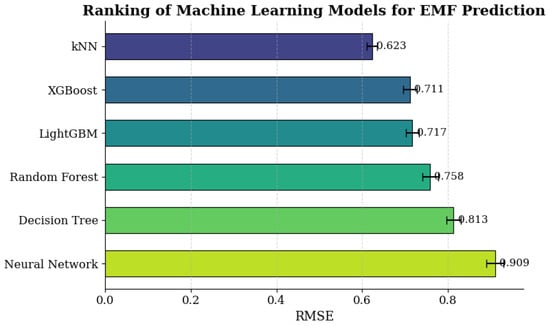
Figure 3.
Comparative Analysis ML Models Ranking Table based on Mean RMSE.
In summary, the results establish a clear ranking order of predictive EMF performance as follows:
- k-Nearest Neighbors: mean RMSE = 0.623153, SD = 0.042993, CI = [0.611236, 0.635070]
- (||)
- XGBoost: mean RMSE = 0.711201, SD = 0.059282, CI = [0.694769, 0.727633]
- (|||)
- LightGBM: mean RMSE = 0.716689, SD = 0.053689, CI = [0.701807, 0.731571]
- (|||)
- Random Forest: mean RMSE = 0.757916, SD = 0.066344, CI = [0.739527, 0.776306]
- (||)
- Decision Tree: mean RMSE = 0.812665, SD = 0.060873, CI = [0.795792, 0.829538]
- ()
- Neural Networks: mean RMSE = 0.909277, SD = 0.070638, CI = [0.889697, 0.928857]
- ()
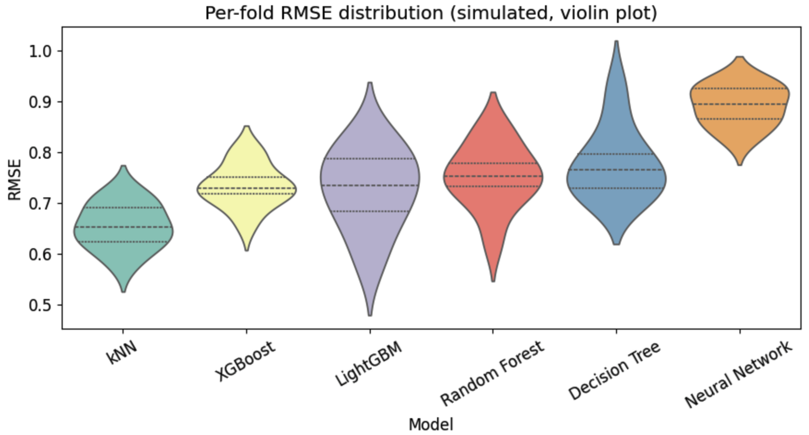
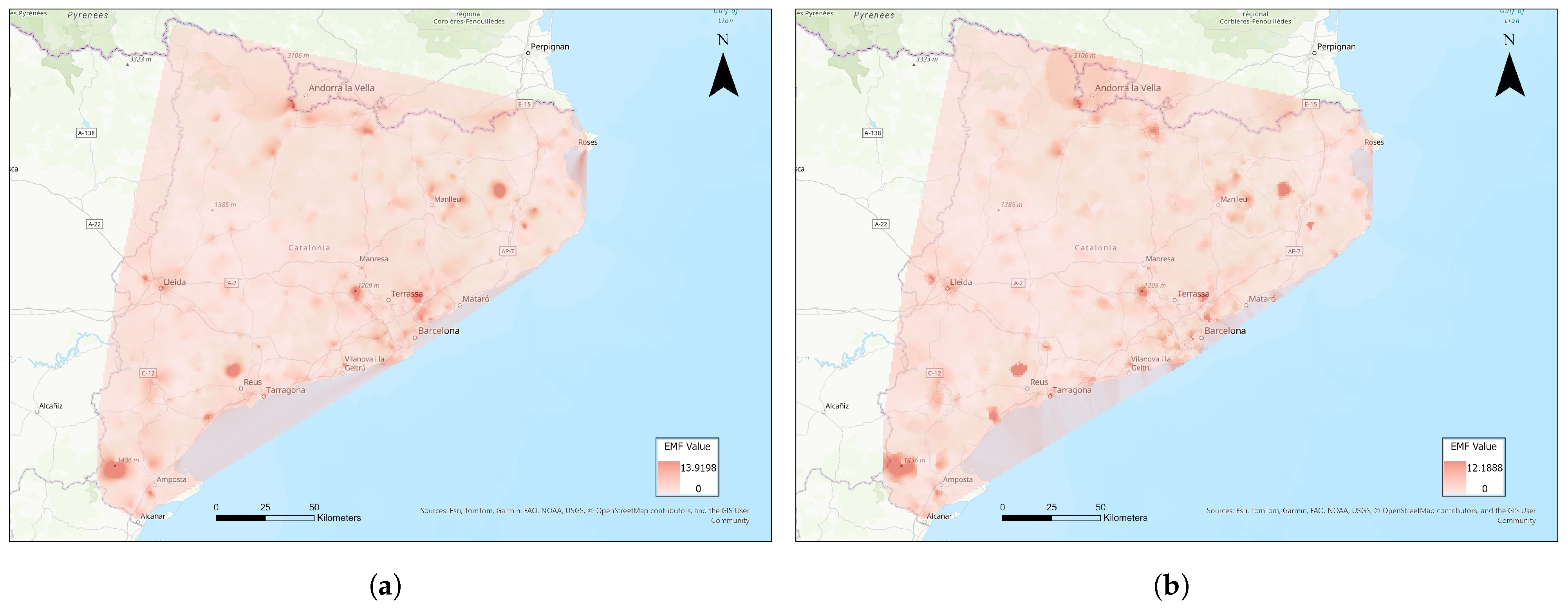
The superior accuracy of kNN highlights the effectiveness of instance-based learning for this specific EMF prediction task, though its computational efficiency may pose limitations for very large datasets. On the other hand, more novel gradient boosting approaches, such as XGBoost and LightGBM, provide a strong trade-off between predictive performance and scalability, while Random Forest remains a robust yet slightly less accurate alternative. Conversely, single-tree and neural architectures require careful hyperparameter refinement-calibration in order to approach the performance of ensemble-based methods. Summing up, these findings suggest that future work should prioritize boosting models or optimized kNN schemes, while indicating the potential of exploring hybrid approaches that integrate the effectiveness of instance-based learning with the interpretability of decision trees and the accuracy of ensemble learning methods. Figure 4 showcase a comparative analysis of RMSEs distributions across all ML modes. Also, the Figure 5 shows how the predicted values are mapped over the area of interest.

Figure 4.
ML Models Per-fold Violin Plots of RMSE Distributions.

Figure 5.
(a) Spatial interpolation of electromagnetic field (EMF) intensity across Catalonia, Spain, using k-NN method (b) Spatial interpolation of electromagnetic field (EMF) intensity across Catalonia, Spain, using XGBoost method.
4.2. XAI Results and Explanations
4.2.1. SHAP
The SHAP (SHapley Additive exPlanations) framework offers a unified, model-agnostic approach for interpreting complex machine learning predictions by quantifying the marginal contribution of each feature to the model’s output. In particular, SHAP decomposes a model’s prediction into additive feature attributions, ensuring both local accuracy and global consistency across instances. The global perspective aggregates feature contributions across all samples to identify the dominant predictors driving EMF variability at the population level. Conversely, the local perspective focuses on individual predictions, explaining how specific feature interactions influence the model’s output for a given observation.
Specifically, in the context of electromagnetic field (EMF) strength prediction, the SHAP dual approach of the above two perspectives facilitate a comprehensive understanding of both the overall model behavior and case-specific explanatory patterns and so, enables a detailed examination of how spatial, demographic, and environmental variables-features influence model outputs, thereby providing transparent and theoretically grounded insights into the underlying decision mechanisms of the employed ML algorithms.
In the subsequent subsections, SHAP results are presented for the top-performing ML models, including k-Nearest Neighbors (kNN) and XGBoost. The global SHAP summary plots (beeswarm plots) illustrate the average magnitude and direction of each feature’s contribution to EMF prediction, while local explanations (waterfall plots) reveal instance-specific deviations and contextual dependencies. This dual analysis enables the identification of consistent explanatory trends across models and environments, forming a robust interpretive basis for assessing predictive performance and environmental significance.
kNN SHAP Analysis
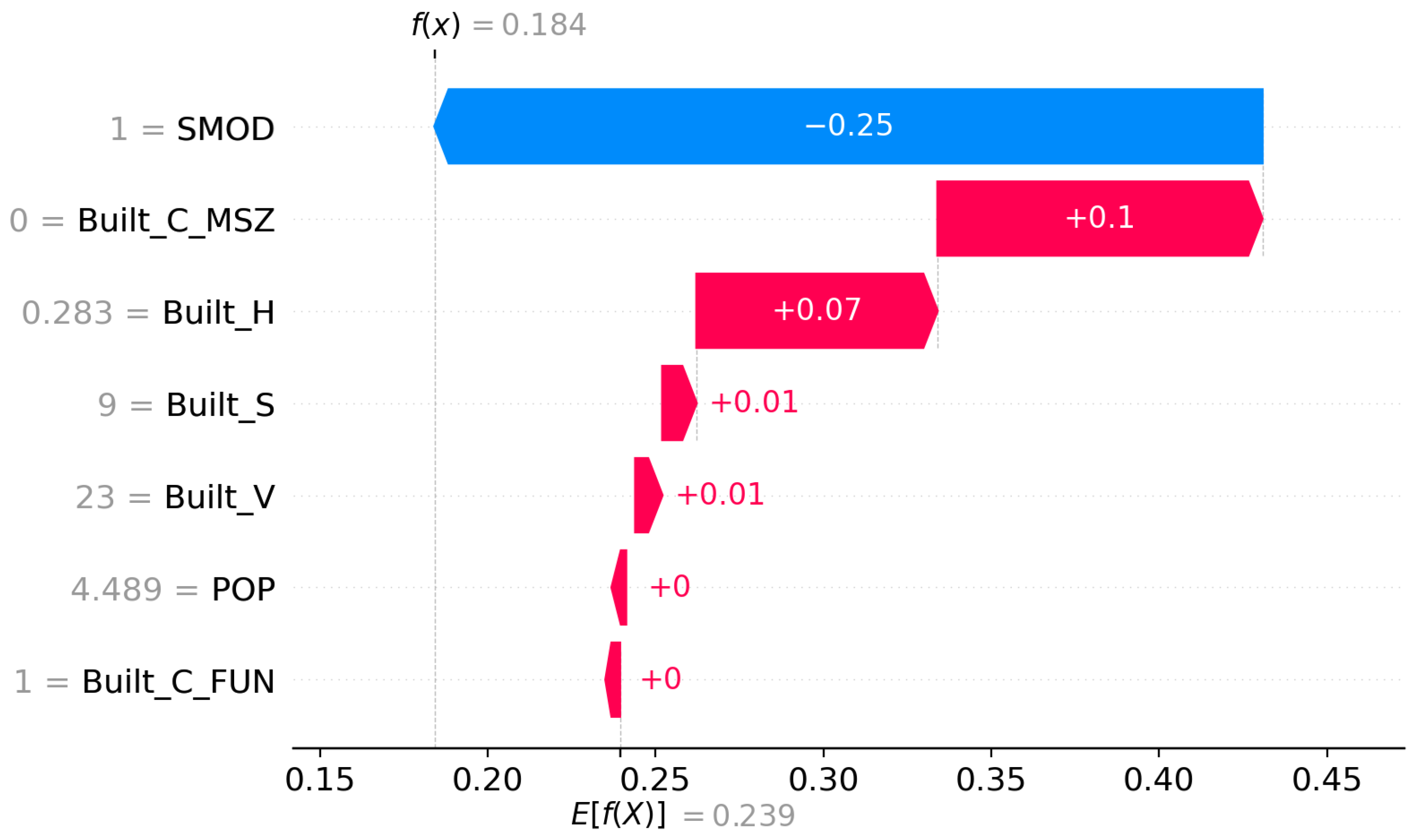
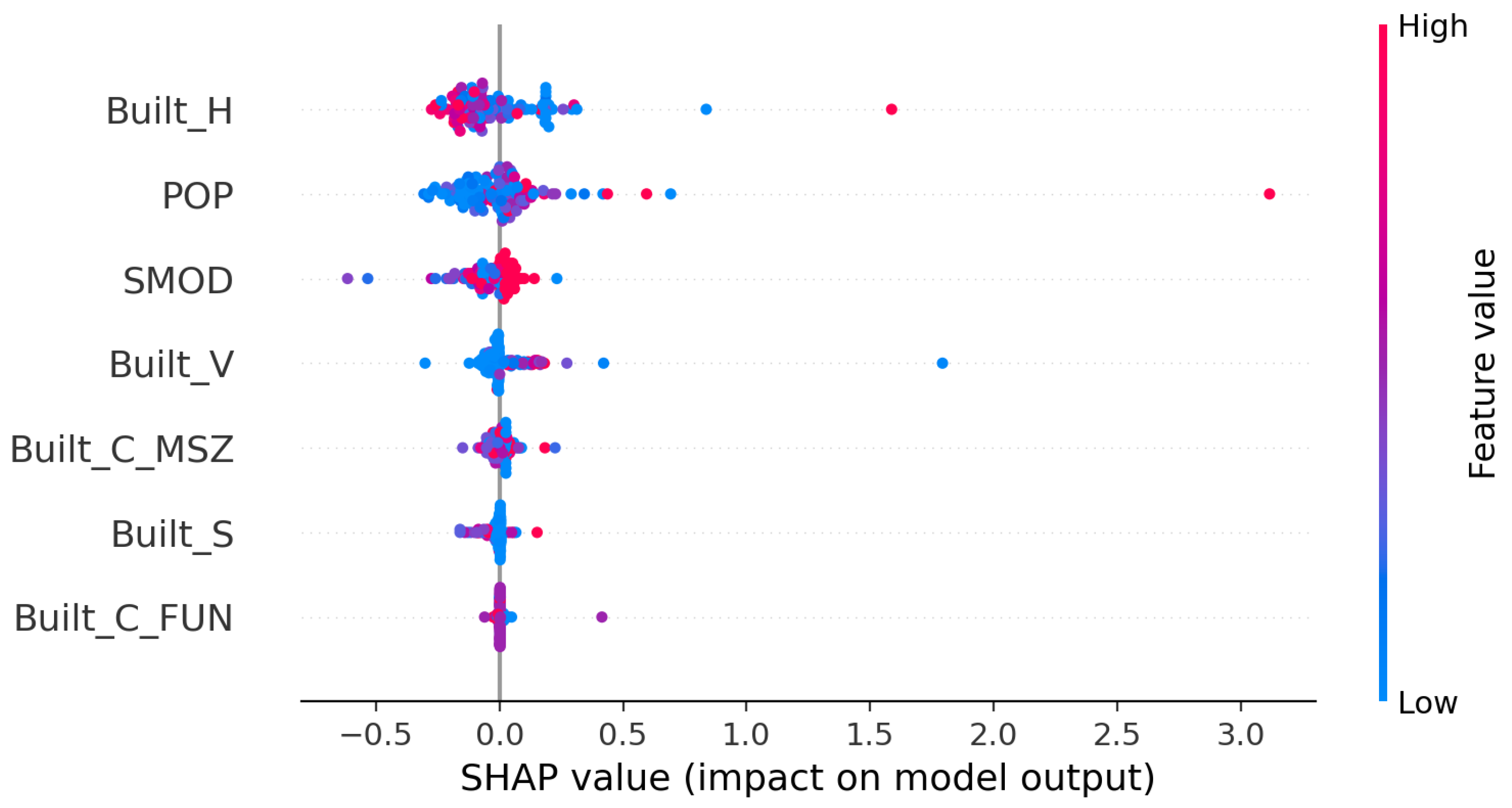
Figure 6 (beeswarm plot) visualizes both the magnitude and directionality of each feature’s impact, whereas Figure 7 (waterfall plot) illustrates the additive effect of the most influential variables for a representative prediction instance. The signed mean SHAP values reflect whether a feature predominantly increases or decreases the predicted electromagnetic field (EMF) strength, while the absolute mean SHAP values capture the overall influence magnitude, independent of direction.
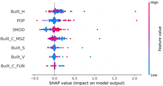
Figure 6.
kNN SHAP Beeswarm Plot.

Figure 7.
kNN SHAP Waterfall Plot.
Among all predictors, SMOD (Degree of Urbanisation) emerges as the most influential variable (Figure 7), displaying the strongest negative SHAP contribution on average. This suggests that areas classified with higher urbanisation degrees correspond to a relative decrease in predicted EMF strength within the kNN model’s local decision structure, possibly due to attenuation effects or signal diffusion associated with denser morphological configurations. Conversely, Built_C_MSZ, representing the Morphological Settlement Zone classification, exerts a positive influence, indicating that denser or morphologically structured settlements tend to elevate EMF predictions, which likely reflects a potential increased infrastructure and emitter density in such zones.
The features Built_H (average building height), Built_S (built-up surface), and Built_V (built-up volume) also show moderate positive contributions, emphasizing the importance of vertical and horizontal development intensity in shaping EMF propagation, whereas the feature variable POP (population density) appears to have a relatively minor but still meaningful impact, consistent with the idea that population distribution serves as an indirect indication for built infrastructure. Finally, Built_C_FUN (residential vs. non-residential functional classification) demonstrates minimal impact, suggesting that functional land-use type alone does not strongly determine EMF variations once structural characteristics are accounted for.
Overall, the SHAP-based interpretability analysis reveals that urban morphology and spatial structural variables, particularly the degree of urbanisation, settlement delineation, and built environment metrics, constitute the most decisive factors in the kNN model’s EMF strength predictions. This evidence underscores the model’s sensitivity to fine-grained geospatial geometric attributes rather than purely demographic factors. From a methodological standpoint, SHAP confirms that the kNN model captures locally heterogeneous spatial geometrical dependencies, reinforcing the value of spatially explicit variables in EMF modeling frameworks.
XGBoost SHAP Analysis
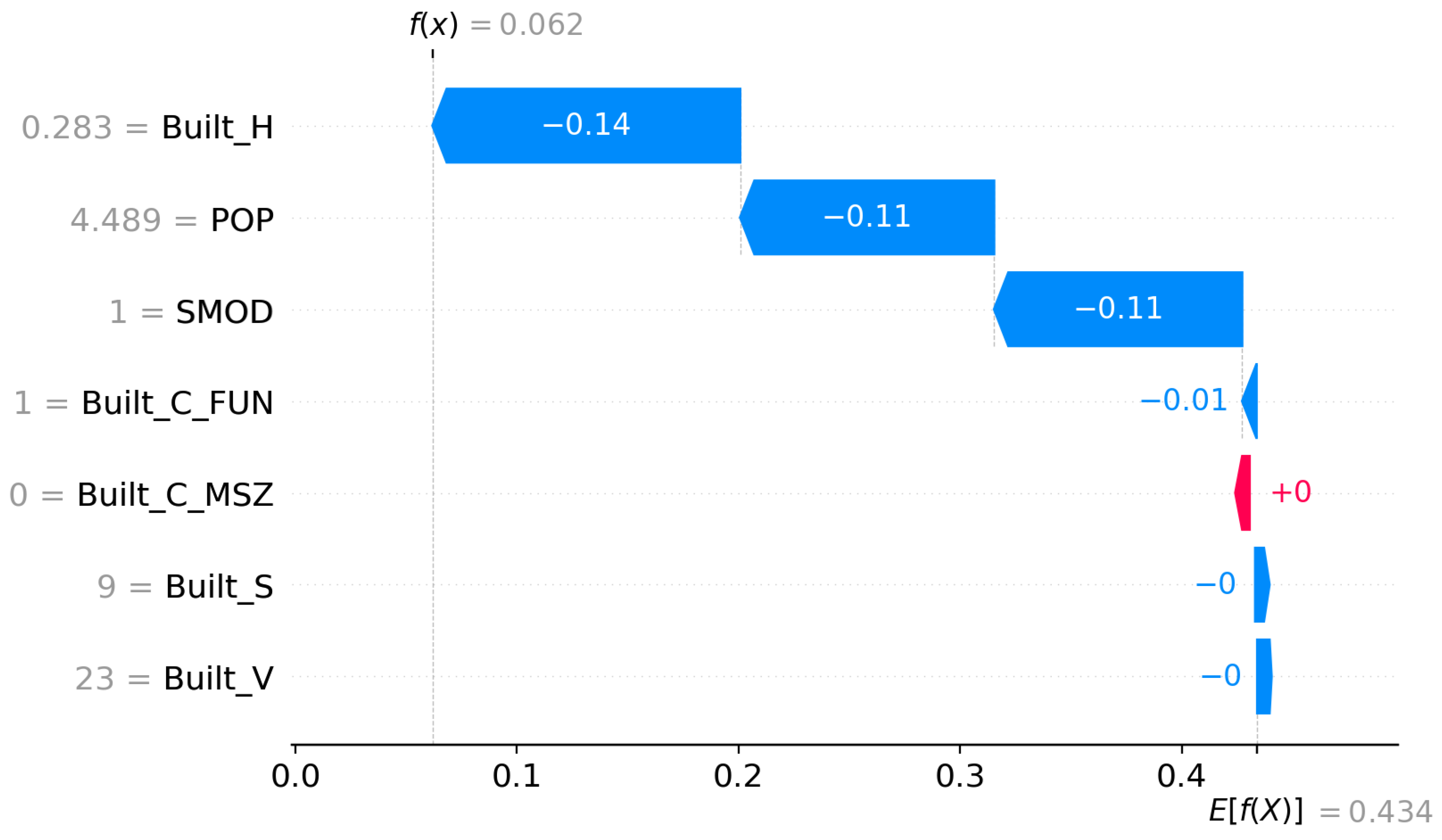
The summary of the XGBoost SHAP analysis as depicted in (beeswarm) plot in Figure 8 visualizes the distribution of SHAP values across all test samples, thereby quantifying both the magnitude and direction of each feature’s effect on the predicted EMF intensity. Meanwhile, the waterfall plot in Figure 9 illustrates a single prediction instance, showing how the cumulative contributions of features shift the prediction from the baseline expectation to the final model output . The signed mean SHAP values reveal whether a feature tends to increase or decrease the predicted EMF, while the absolute mean SHAP values highlight its overall importance in shaping the model output.
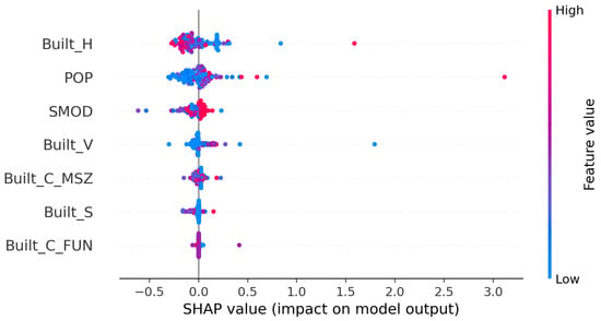
Figure 8.
XGBoost SHAP Beeswarm Plot.
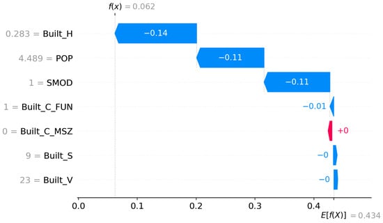
Figure 9.
XGBoost SHAP Waterfall Plot.
Among the examined predictors, Built_H (building height), POP (population density), and SMOD (degree of urbanisation) emerge as the most influential variables, as clearly illustrated in Figure 9, in determining the model’s predictions. The SHAP values indicate that higher building heights and higher population densities generally lead to a decrease in predicted EMF levels, as shown by the negative SHAP contributions for these variables. This pattern can be attributed to the signal attenuation and scattering effects introduced by taller structures and densely populated urban cores, which can obstruct direct line-of-sight propagation. Similarly, SMOD, representing the urbanisation level, exerts a negative influence, suggesting that highly urbanized zones, often characterized by dense building clusters and infrastructure, tend to experience lower EMF intensities at ground level due to increased multipath fading and signal absorption.
On the other hand, features related to morphological classification, such as the variables Built_C_MSZ (Morphological Settlement Zone) and Built_C_FUN (functional classification of the built environment), exhibit comparatively smaller yet non-negligible impacts. The weak positive or near-zero contributions of these variables suggest that while the categorical partitioning of urban morphology provides structural context, it alone does not substantially modify EMF predictions beyond the physical characteristics that already captured by building height and surface data. Similarly, Built_S (built-up surface) and Built_V (built-up volume) show marginal contributions, reinforcing the idea that geometric and structural aspects of the urban fabric, although interacting with EMF propagation mechanisms, still remain secondary to the building height and population-related attenuation factors.
Overall, the SHAP analysis confirms that structural and demographic urban characteristics jointly govern EMF distribution, with XGBoost effectively capturing the nonlinear dependencies between physical urban morphology and exposure levels. The model assigns higher importance to attenuative factors (e.g., height, density) rather than purely spatial classifications, aligning well with established radio propagation theory. From an interpretability standpoint, these results validate the physical plausibility of the XGBoost model’s learning behavior, where the identified feature effects are consistent with empirical observations in urban electromagnetic environments, thereby enhancing confidence in its predictive transparency and reliability.
SHAP Discussion
Comparative dual SHAP interpretations reveal that the k-Nearest Neighbors (kNN) and XGBoost models achieve similar predictive accuracy but through fundamentally different explanatory mechanisms. The kNN model exhibits heightened sensitivity to spatial and morphological-topological structure, relying on neighborhood similarity in the feature space to infer electromagnetic field (EMF) strength. Its predictions are primarily influenced by local contextual features, particularly morphological indicators such as urban form and settlement classification, reflecting the model’s instance-based reasoning and dependence on spatial geometric distance-based proximity.
In contrast, the XGBoost model emphasize on physical attenuation dynamics and quantitative urban metrics, capturing complex nonlinear interactions and cumulative effects among structural and demographic variables. This behavior aligns more closely with theoretical signal propagation principles, as the model generalizes more effectively across heterogeneous urban settings by learning hierarchical relationships rather than specific localized associations.
Together, these complementary interpretability profiles demonstrate that kNN encodes better upon spatial similarity while XGBoost learns more effective parametric attenuation functions, two distinct but yet potential synergistic approaches to modeling EMF variability. Integrating both local (kNN-driven) and global (XGBoost-driven) interpretability perspectives yields a more comprehensive and physically consistent understanding of EMF behavior in urban environments, thereby advancing transparent, data-driven methodologies for environmental monitoring and urban planning.
4.2.2. LIME
The LIME (Local Interpretable Model-Agnostic Explanations) framework provides a complementary perspective to SHAP by focusing explicitly on local interpretability—that is, understanding the reasoning behind individual model predictions. Unlike SHAP, which derives globally consistent feature attributions based on cooperative game theory, LIME approximates the complex behavior of a trained model in the vicinity of a specific instance by fitting a locally linear alternative substitute model. This approximation allows for the identification of the most influential features contributing to a given prediction, thereby offering interpretable, human-readable insights into the local decision boundaries of non-linear models.
Specifically, in the context of electromagnetic field (EMF) strength prediction, LIME facilitates the examination of localized environmental, demographic, and infrastructural conditions that drive model predictions for specific spatial locations. This approach is particularly valuable for identifying context-sensitive deviations that may not be visible in more global XAI approaches like SHAP. By combining LIME’s fine-grained local analysis with SHAP’s globally consistent attributions, a comprehensive interpretability framework is achieved that can support both the validation of model behavior and the transparent communication of EMF prediction results for scientific and regulatory purposes. In correspondence to SHAP analysis, the following subsections present the LIME results for the top-performing ML models, k-Nearest Neighbors (kNN) and XGBoost.
kNN LIME Analysis
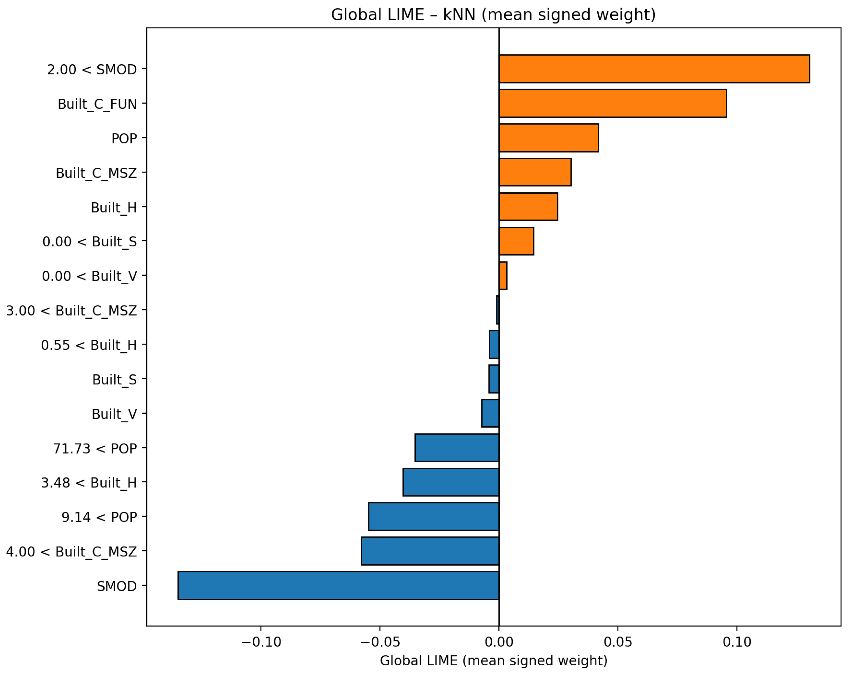
Consecutive to the SHAP-based interpretability analysis, Local Interpretable Model-Agnostic Explanations (LIME) was employed in order to complement and examine feature contributions for the k-Nearest Neighbors (kNN) model. LIME was applied in a global aggregation framework, wherein instance-level explanations were averaged across the test set to obtain both absolute mean weights Figure 10 (indicating importance magnitude irrespective of direction) and signed mean weights Figure 11 (denoting whether features systematically increase or decrease EMF predictions). This dual representation provides a richer interpretability perspective, capturing the stability, strength, and polarity of each predictor’s influence on the urban electromagnetic field (EMF) estimations.
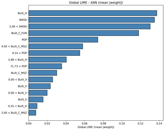
Figure 10.
LIME - kNN Global Absolute Values Feature Importance.

Figure 11.
LIME - kNN Global Signed Values Feature Importance.
The LIME absolute mean weights analysis profile highlights Built_H (building height), SMOD (degree of urbanization), and Built_C_FUN (urban functional classification) as dominant drivers of kNN predictions, followed closely by POP (population density) and Built_C_MSZ (morphological settlement zoning), which collectively suggest that both vertical density and urban planning topology are central determinants in EMF variability. Built form intensity feature variables such as, Built_V (volume) and Built_S (surface area), exhibit smaller but nontrivial contributions, reflecting their secondary role in shaping propagation environments. Overall, the absolute LIME map reinforces the hypothesis that the kNN model relies primarily on local morphological and socio-spatial gradients, consistent with its distance-based learning nature.
The signed LIME contributions (Figure 11) reveal coherent directional patterns. Higher values of Built_H, POP, and SMOD tend to increase EMF levels, consistent with urban densification leading to heightened wireless infrastructure density and reflective interference effects. In contrast, certain categories of Built_C_MSZ and low-rise built environments exhibit negative directional effects, suggesting attenuation or less intensive radiative environments in suburban or semi-urban contexts. The consistent polarity of Built_H and SMOD across most instances underscores their robust explanatory power in shaping EMF exposure gradients, while the mixed-sign behavior of built-form intensity variables (Built_S and Built_V) reflects context-dependent effects, likely driven by variations in infrastructure placement, open-space fragmentation, and various micro-propagation phenomena. Collectively, the LIME interpretations confirm the spatially-adaptive and locally sensitive nature of kNN, which leverages micro-scale morphological attributes to interpolate EMF levels.
XGBoost LIME Analysis
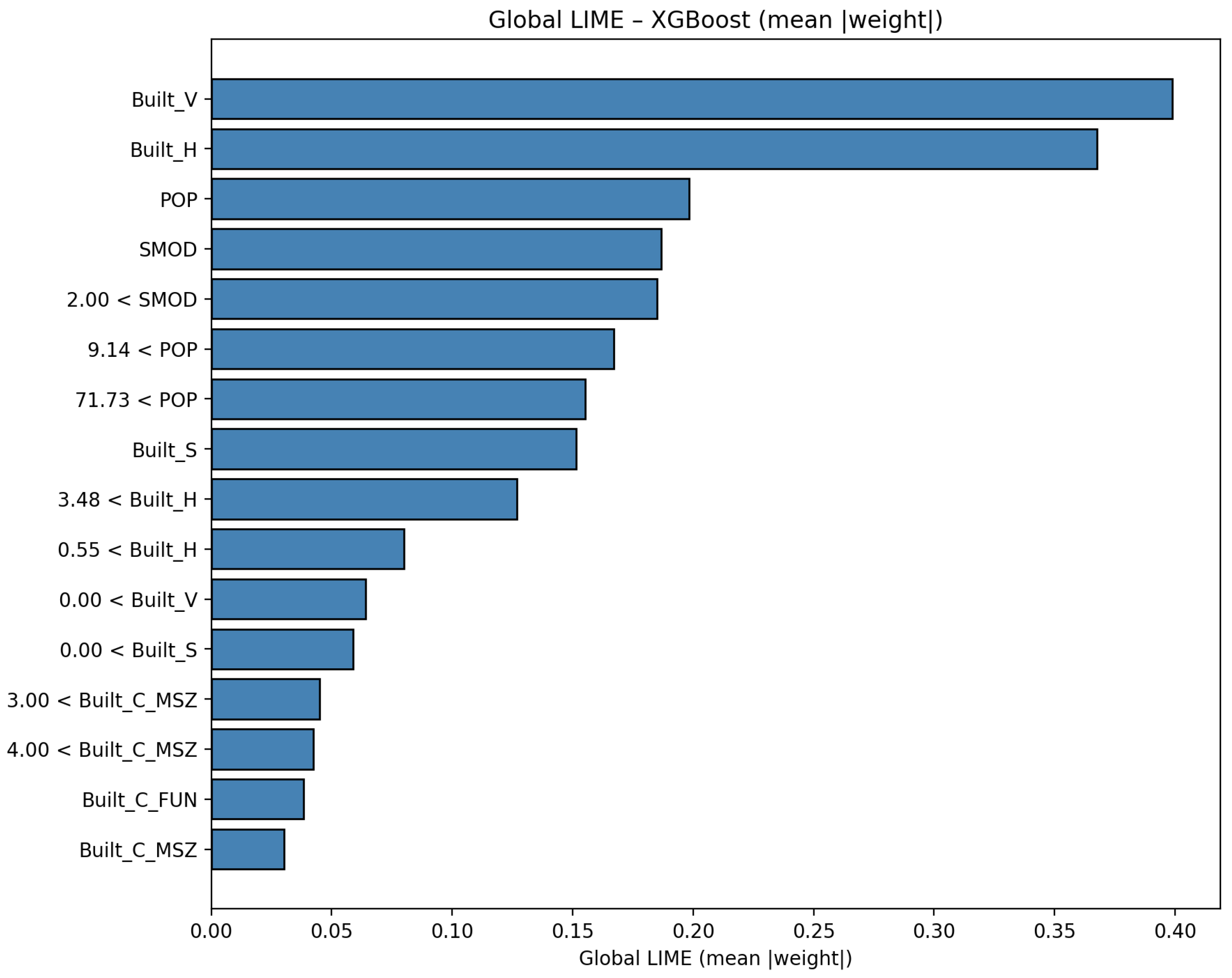
LIME-based interpretability analysis was performed in order to elucidate how the XGBoost model leverages geospatial and morphological urban indicators to predict electromagnetic field (EMF) levels. The global mean absolute LIME weights (Figure 12) reveal that Built_V (built-up volume) and Built_H (building height) emerge as the most influential spatial predictors, followed closely by POP (population density) and SMOD (degree of urbanisation). This dominance indicates that three-dimensional urban morphology and population intensity act as primary determinants shaping EMF variability. The importance of Built_V and Built_H implies a strong association between vertical structural complexity and electromagnetic propagation dynamics, aligning well with radiofrequency propagation theory wherein higher and denser built forms induce multipath effects, signal obstruction, and power variations. Similarly, the prominence of POP and SMOD underscores that densely populated urban cores, which tend to exhibit intensive telecommunication activity and infrastructure concentration, drive higher EMF exposure levels.
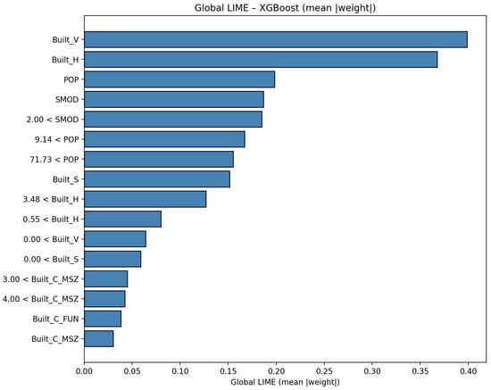
Figure 12.
LIME - XGBoost Global Absolute Values Feature Importance.
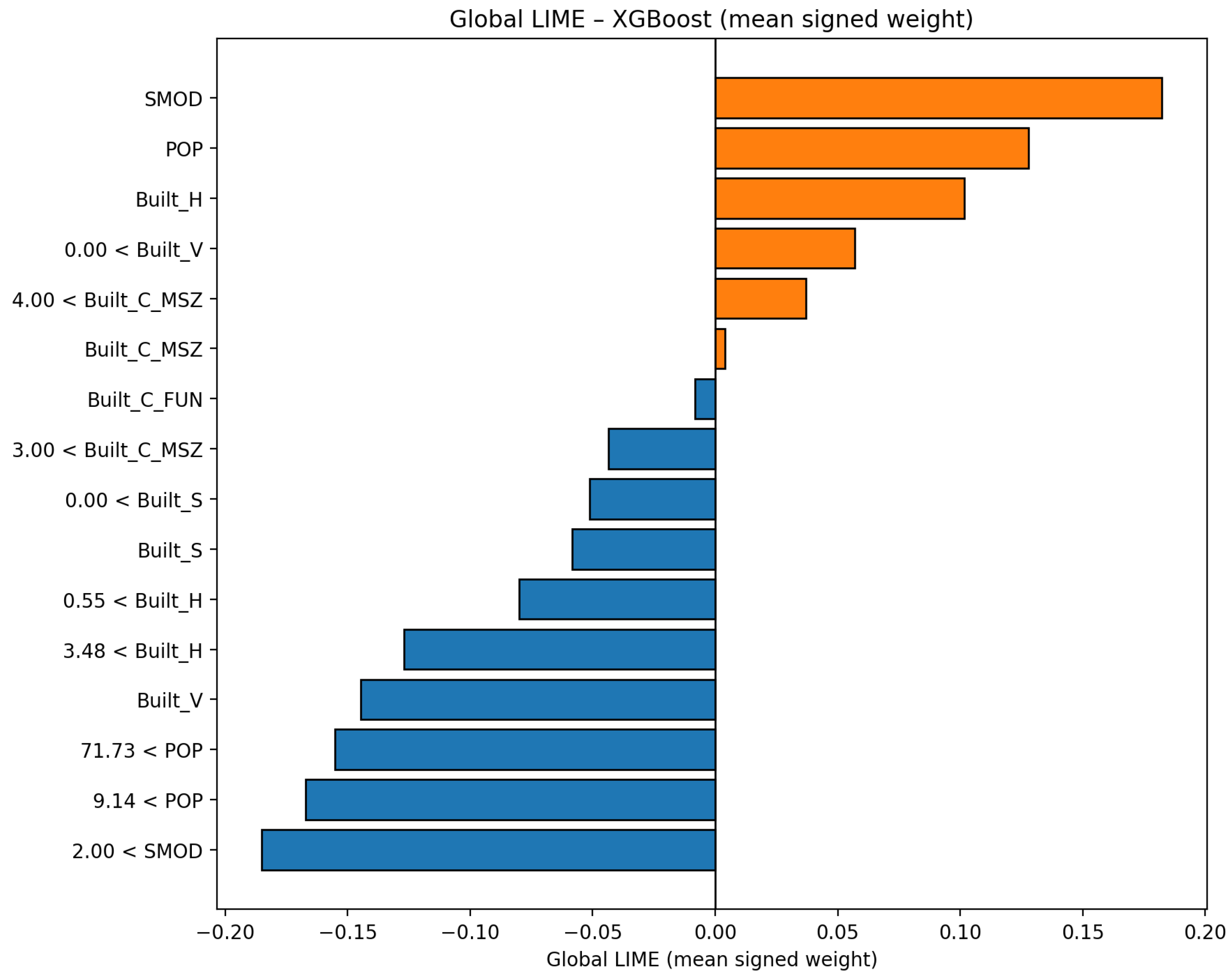
The signed LIME weights (Figure 13) provide insight into directionality. SMOD, POP, and Built_H predominantly exhibit positive signed effects, suggesting that higher values of these features consistently increase model predictions—i.e., contribute to elevated EMF intensity. In contrast, Built_V demonstrates a mixed effect profile: while highly ranked in absolute magnitude, its signed values oscillate around zero across spatial samples, indicating heterogeneous influence that varies by urban context. This pattern reflects physical reality, where vertical density may either attenuate or amplify field strength depending on line-of-sight availability, antenna configuration, and propagation pathways. Built_C_MSZ (settlement morphology classification) and Built_C_FUN (functional class of built space) appear less influential overall but still contribute meaningfully to local decision boundaries, particularly in delineating residential vs. non-residential urban fabric, which indirectly governs telecom antenna distribution and usage patterns.
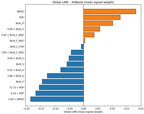
Figure 13.
LIME—XGBoost Global Signed Values Feature Importance.
Collectively, the LIME results demonstrate that the XGBoost model learns coherent, physically interpretable associations grounded in urban morphology structure allocation and population density. The convergence of high absolute importance for Built_V, Built_H, POP, and SMOD across diverse local samples reinforces the robustness of these predictors as primary drivers of EMF exposure spatial heterogeneity. The subtle positive/negative balance for some variables highlights the context-dependent nature of RF propagation, where interactions between terrain, built form, and antenna topology produce nonlinear effects. These findings validate the model’s capacity to reflect real-world physical propagation mechanisms while also providing transparent local explanations that support regulatory, environmental, and urban planning applications.
LIME Discussion
The LIME analysis provides complementary insights into the interpretive behavior of the kNN and XGBoost models by examining feature contributions at the individual-prediction level. Similar to the SHAP findings, both models consistently identify key built-environment and demographic variables, particularly Built_H (building height), Built_V (built volume), Built_S (built surface area) and POP (population density), as the most dominant predictors of EMF intensity. This convergence reinforces the central role of vertical urban form structures and population concentration in shaping radio-frequency propagation electrodynamics.
For the kNN model, the largest LIME attribution magnitudes are associated with Built_H, SMOD, and Built_C_FUN, followed by POP and Built_C_MSZ. Signed contributions reveal context-dependent influences, where certain urban morphologies increase EMF strength while others attenuate it depending on local neighborhood topological similarity. This behavior is consistent with kNN’s instance-based learning paradigm, wherein predictions are strongly shaped by the characteristics of proximate observations. As a result, kNN exhibits more spatially heterogeneous and locally sensitive interpretability, making it particularly informative for micro-scale EMF variation in highly diverse urban settings.
In contrast, XGBoost demonstrates a more structured and globally stable feature attribution pattern. Built_V and Built_H dominate the local explanations, with POP and SMOD also contributing consistently across instances. Directional effects for these variables align closely with already establised theoretical expectations: taller and denser urban environments, which often associated with increased antenna density and multipath propagation, exert strong influence on EMF levels. Compared to kNN, XGBoost yields smoother, more coherent interpretive profiles, reflecting its increased capacity to capture more complex nonlinear, system-level interactions rather than purely local distance-based analogies. Overall, LIME confirms that while kNN provides granular, location-specific interpretability, XGBoost delivers more consistent and physically aligned explanations, resulting in two complementary interpretive paradigms for urban EMF analysis. Together, these LIME results demonstrate that combining instance-level, context-sensitive explanations with broader model-based insights yields a more complete and operationally meaningful understanding of EMF prediction behavior, reinforcing the value of localized interpretability for urban exposure assessment and decision-support applications.
4.2.3. Comparative Analysis Explainable AI Models
A comparative analysis evaluation of SHAP and LIME was conducted in order to elucidate the interpretability characteristics of the employed machine learning models and to assess the consistency, stability, and physical plausibility of feature attributions in the context of EMF field prediction. Both frameworks identified urban morphology and demographic intensity as primary drivers of EMF variability, with highly consistent emphasis across models on variables capturing three-dimensional built form and urbanisation. Specifically, Built_H (building height), Built_V (built volume), POP (population density), and SMOD (degree of urbanisation) emerged as dominant predictors under both methods, reinforcing that vertical density, infrastructure concentration, and population-driven network intensity jointly shape radiofrequency propagation in dense urban environments. Secondary variables such as Built_S, Built_C_MSZ, and Built_C_FUN provided additional structural context, though with comparatively weaker influence. This convergence across SHAP and LIME substantiates the physical plausibility of the learned EMF patterns, aligning model interpretability outcomes with underlying electromagnetic propagation theory.
Despite this overarching consistency, SHAP and LIME exhibited complementary interpretive behaviors reflecting their methodological underpinnings. SHAP provided globally stable, additive attributions with clear decomposition of prediction contributions, enabling systematic quantification of global importance patterns while preserving local fidelity. This was particularly evident for XGBoost, where SHAP exposed coherent attenuation patterns associated with increasing building height and population density, alongside structured nonlinear interactions across the urban morphology. LIME, by contrast, emphasized high-resolution local interpretability, capturing spatially varying effects driven by neighborhood-specific morphology—particularly pronounced in kNN, where instance-based reasoning produced heterogeneous but physically meaningful feature impacts tied to local similarity relationships. Thus, while SHAP offered robust and globally consistent explanations suitable for model benchmarking and scientific inference, LIME revealed contextual micro-dynamics valuable for localized environmental assessment and scenario-specific interpretation.
Overall, the comparative analysis demonstrates that SHAP and LIME act as complementary interpretability mechanisms. SHAP excels in establishing global causal consistency and theoretical conformity, whereas LIME enhances granularity in local diagnostic interpretation. The combined deployment of both methods results in a comprehensive transparency framework, enabling robust validation of model behavior, improved credibility of EMF predictions, and enhanced interpretive utility for urban-scale electromagnetic exposure monitoring and decision-support applications.
Table 9 and Figure 14 summarize the explainability results obtained across SHAP and LIME, where feature importance analysis of kNN and XGBoost ML methods consistently highlight Built_H, Built_V, and population density POP as the primary drivers of EMF field variability, with SMOD providing additional contextual differentiation of urban form topology. These findings confirm that vertical urban morphology and demographic intensity exert the strongest influence on RF propagation patterns, reinforcing the physical plausibility and robustness of the learned predictive relationships. As shown in the newly added Figure 14, we summarize the feature-importance patterns across kNN and XGBoost models using a heatmap that integrates both SHAP and LIME evaluations. In order to visualize the qualitative feature-importance categories in a unified manner, we encoded each textual level into an ordinal numerical scale as follows:

Table 9.
Feature importance alignment across kNN and XGBoost models using SHAP and LIME.

Figure 14.
Combined SHAP and LIME feature importance and consistency across kNN and XGBoost models.
This mapping enables consistent graphical representation of importance intensity across models and interpretability methods.
5. Conclusions
This study conducted a rigorous, head-to-head evaluation of six machine-learning model paradigms for urban electric field (EMF) strength prediction, Neural Networks (NN), k-Nearest Neighbors (kNN), Decision Trees (DTs), Random Forest (RF), LightGBM, and XGBoost, augmented with model-agnostic interpretability via SHAP and LIME. Using cross-validated root mean squared error (RMSE) as the principal performance evaluation metric, we found a clear accuracy hierarchy: kNN achieved the lowest error (mean RMSE = 0.623153), followed by XGBoost (0.711201), LightGBM (0.716689), Random Forest (0.757916), Decision Trees (0.812665), and Neural Networks (0.909277). While the two gradient-boosting ensembles approached kNN’s accuracy with stronger scalability properties, the instance-based learner retained a decisive advantage on the present dataset, indicating a pronounced role of local similarity structure in EMF spatial variability.
The interpretability analysis converged on a consistent physical interpretation. Across the top performing model methods, Built_H (building height), Built_V (built volume), POP (population density), and SMOD (degree of urbanisation) emerged as primary determinants of EMF levels, with Built_S, Built_C_MSZ, and Built_C_FUN providing secondary structural context attributions. SHAP exposed globally stable attribution patterns, particularly for XGBoost, highlighting attenuation and propagation effects tied to vertical density and demographic intensity, whereas LIME illuminated locally contingent behaviors, especially for kNN, where neighborhood-specific morphology modulates predictions. The alignment of SHAP and LIME with radio-propagation intuition strengthens confidence in the learned relations and supports the scientific validity of the models’ decision processes.
kNN provides the highest accuracy and strong local adaptability, although it can be memory-intensive at large scales. XGBoost and LightGBM offer an effective balance of accuracy, robustness, and inference speed, provided that regularization is carefully tuned. Random Forest remains a reliable baseline but is less accurate than boosting methods, while single Decision Trees and the tested Neural Networks underperformed in complex urban environments.
These findings have practical implications for EMF exposure assessment. When maximum accuracy is required and computational resources allow, distance-weighted kNN with moderate neighborhood sizes (–25) is recommended. For applications prioritizing scalability and generalization, XGBoost and LightGBM provide near-optimal accuracy with faster performance. The consistent influence of building height, built volume, population density, and urbanization degree further highlights their importance in shaping EMF patterns.
In summary, this study establishes a strong benchmark for interpretable EMF modeling. kNN achieved the best accuracy, XGBoost and LightGBM offered scalable high performance, and the SHAP–LIME analysis yielded coherent, physically meaningful explanations. Together, these results support more transparent EMF monitoring and guide future improvements in data enrichment, model design, and urban planning applications.
Author Contributions
Conceptualization, Y.K. and D.K.; methodology, Y.K.; software, C.C.; validation, I.G., D.K. and Y.K.; formal analysis, Y.K.; data curation, C.C.; writing—original draft preparation, I.G.; writing—review and editing, Y.K.; visualization, C.C.; supervision, Y.K.; project administration, D.K. All authors have read and agreed to the published version of the manuscript.
Funding
This research received no external funding.
Data Availability Statement
The original contributions presented in this study are included in the article. Further inquiries can be directed to the corresponding author.
Conflicts of Interest
The authors declare no conflicts of interest.
Abbreviations
The following abbreviations are used in this manuscript:
| AI | Artificial Intelligence |
| ANN | Artificial Neural Network |
| CNN | Convolutional Neural Network |
| DNN | Deep Neural Network |
| DT | Decision Tree |
| EMF | Electromagnetic Field |
| GBDT | Gradient Boosting Decision Tree |
| GHSL | Global Human Settlement Layer |
| kNN | k-Nearest Neighbors |
| LIME | Local Interpretable Model-agnostic Explanations |
| LightGBM | Light Gradient Boosting Machine |
| ML | Machine Learning |
| RF | Random Forest |
| REM | Radio Environment Mapping |
| RMSE | Root Mean Squared Error |
| SHAP | SHapley Additive exPlanations |
| SVM | Support Vector Machine |
| XAI | Explainable Artificial Intelligence |
| XGBoost | Extreme Gradient Boosting |
References
- Chen, W.; Lin, X.; Lee, J.; Toskala, A.; Sun, S.; Chiasserini, C.F.; Liu, L. 5G-Advanced Toward 6G: Past, Present, and Future. IEEE J. Sel. Areas Commun. 2023, 41, 1592–1619. [Google Scholar] [CrossRef]
- Polymeni, S.; Plastras, S.; Skoutas, D.N.; Kormentzas, G.; Skianis, C. The Impact of 6G-IoT Technologies on the Development of Agriculture 5.0: A Review. Electronics 2023, 12, 2651. [Google Scholar] [CrossRef]
- Chataut, R.; Nankya, M.; Akl, R. 6G Networks and the AI Revolution—Exploring Technologies, Applications, and Emerging Challenges. Sensors 2024, 24, 1888. [Google Scholar] [CrossRef] [PubMed]
- Korkmaz, E.; Aerts, S.; Coesoij, R.; Bhatt, C.R.; Velghe, M.; Colussi, L.; Land, D.; Petroulakis, N.; Spirito, M.; Bolte, J. A comprehensive review of 5G NR RF-EMF exposure assessment technologies: Fundamentals, advancements, challenges, niches, and implications. Environ. Res. 2024, 260, 119524. [Google Scholar] [CrossRef] [PubMed]
- Iakovidis, S.; Manassas, A.; Apostolidis, C.; Samaras, T. 5G EMF Exposure at 3.6 GHz in Greece Using Data from Frequency-Selective Monitoring Sensors. Bioelectromagnetics 2025, 46, e70008. [Google Scholar] [CrossRef]
- Veludo, A.F.; Stroobandt, B.; Bladel, H.V.; Sandoval-Diez, N.; Deprez, K.; Aerts, S.; Chikha, W.B.; Wiart, J.; Vecsei, Z.; Necz, P.P.; et al. Assessing radiofrequency electromagnetic field exposure in multiple microenvironments across ten European countries with a focus on 5G. Environ. Int. 2025, 200, 109540. [Google Scholar] [CrossRef]
- Bladel, H.V.; Stroobandt, B.; Veludo, A.F.; Deprez, K.; Röösli, M.; Tognola, G.; Parazzini, M.; Thuróczy, G.; Polańska, K.; Politański, P.; et al. RF-EMF exposure assessment with add-on uplink exposure sensor in different microenvironments in seven European countries. Environ. Int. 2025, 197, 109368. [Google Scholar] [CrossRef]
- World Health Organization. Electromagnetic Fields (EMF). WHO Web Page (Overview and Ongoing Risk Assessment). Available online: https://www.who.int/health-topics/electromagnetic-fields?utm_source=chatgpt.com#tab=tab_1 (accessed on 22 November 2025).
- International Commission on Non-Ionizing Radiation Protection (ICNIRP). Guidelines for limiting exposure to electromagnetic fields (100 kHz–300 GHz). Health Phys. 2020, 118, 483–524. Available online: https://www.icnirp.org (accessed on 22 November 2025).
- Ramirez-Vazquez, R.; Escobar, I.; Vandenbosch, G.A.E.; Arribas, E. Personal exposure to radiofrequency electromagnetic fields: A comparative analysis of international, national, and regional guidelines. Environ. Res. 2024, 246, 118124. [Google Scholar] [CrossRef]
- Kiouvrekis, Y.; Alexias, A.; Softa, V.; Alkhorayef, M.; Sulieman, A.; Tyrakis, C.; Kappas, C. Extremely Low Frequency Electromagnetic Exposure Assessment in Schools: A Statistical Analysis of Urban and Semi-Urban Areas. Radiat. Prot. Dosim. 2021, 194, 76–81. [Google Scholar] [CrossRef]
- Birks, L.E.; Struchen, B.; Eeftens, M.; van Wel, L.; Huss, A.; Gajšek, P.; Kheifets, L.; Gallastegi, M.; Dalmau-Bueno, A.; Estarlich, M.; et al. Spatial and temporal variability of personal environmental exposure to radio frequency electromagnetic fields in children in Europe. Environ. Int. 2018, 117, 204–214. [Google Scholar] [CrossRef]
- Ramirez-Vazquez, R.; Gonzalez-Rubio, J.; Arribas, E.; Najera, A. Characterisation of personal exposure to environmental radiofrequency electromagnetic fields in Albacete (Spain) and assessment of risk perception. Environ. Res. 2019, 172, 109–116. [Google Scholar] [CrossRef] [PubMed]
- Panagiotakopoulos, T.; Kiouvrekis, Y.; Misthos, L.-M.; Kappas, A.C. RF-EMF Exposure Assessments in Greek Schools to Support Ubiquitous IoT-Based Monitoring in Smart Cities. IEEE Access 2021, 11, 7145–7156. [Google Scholar] [CrossRef]
- Veludo, A.F.; Stroobandt, B.; Bladel, H.V.; Sandoval-Diez, N.; Guxens, M.; Joseph, W.; Röösli, M. Exploring RF-EMF levels in Swiss microenvironments: An evaluation of environmental and auto-induced downlink and uplink exposure in the era of 5G. Environ. Res. 2025, 266, 120550. [Google Scholar] [CrossRef] [PubMed]
- Stroobandt, B.; Bladel, H.V.; Veludo, A.F.; Deprez, K.; Aerts, S.; Verloock, L.; Thuróczy, G.; Politanski, P.; Polanska, K.; Tognola, G.; et al. Auto-induced uplink 4G and 5G RF-EMF exposure assessment using a network monitoring application in different microenvironments across seven European countries. Environ. Res. 2025, 270, 121029. [Google Scholar] [CrossRef]
- Benke, G.; Abramson, M.J.; Brzozek, C.; McDonald, S.; Kelsall, H.; Sanagou, M.; Zeleke, B.M.; Kaufman, J.; Brennan, S.; Verbeek, J.; et al. The effects of radiofrequency exposure on cognition: A systematic review and meta-analysis of human observational studies. Environ. Int. 2024, 188, 108779. [Google Scholar] [CrossRef]
- Verbeek, J.; Zeeb, H.; van Deventer, E.; Ijaz, S.; Doré, J.F.; Driessen, S.; Roth, N.; Whaley, P. Systematic reviews and meta-analyses for the WHO assessment of health effects of exposure to radiofrequency electromagnetic fields, an introduction. Environ. Int. 2025, 203, 109751. [Google Scholar] [CrossRef]
- Maloku, H.; Fazliu, Z.L.; Dobruna, J.; Ibrani, M. A Measurement-Based Trade-Off Analysis of EMF Exposure Levels and QoS in Mobile Networks. IEEE Access 2025, 13, 94354–94369. [Google Scholar] [CrossRef]
- Calderon, C.; Addison, D.; Peyman, A. In-Situ Measurements of Radiofrequency Electromagnetic Fields Measurements Around 5G Macro Base Stations in the UK. Bioelectromagnetics 2025, 46, e70012. [Google Scholar] [CrossRef]
- Paniagua-Sánchez, J.M.; García-Cobos, F.J.; Rufo-Pérez, M.; Jiménez-Barco, A. Large-area mobile measurement of outdoor exposure to radio frequencies. Sci. Total Environ. 2023, 877, 162852. [Google Scholar] [CrossRef]
- Onishi, T.; Esaki, K.; Tobita, K.; Ikuyo, M.; Taki, M.; Watanabe, S. Large-Area Monitoring of Radiofrequency Electromagnetic Field Exposure Levels from Mobile Phone Base Stations and Broadcast Transmission Towers by Car-Mounted Measurements around Tokyo. Electronics 2023, 12, 1835. [Google Scholar] [CrossRef]
- Arribas, E.; Escobar, I.; Martinez-Plaza, A.; Rufo-Pérez, M.; Jimenez-Barco, A.; Paniagua-Sánchez, J.M.; Marín, P.; Ramirez-Vazquez, R. RF-EMF Exposure Assessment: Comparison of Measurements in Airports and Flights with and Without Wi-Fi Service. Sensors 2025, 25, 6710. [Google Scholar] [CrossRef] [PubMed]
- Guillén-Pina, J.; Pérez-Aracil, J.; Chocano-del-Cerro, R.; Sánchez-Montero, R.; López-Espí, P.-L.; Salcedo-Sanz, S. Efficient design of electromagnetic field exposure maps with multi-method evolutionary ensembles. Environ. Res. 2025, 278, 121636. [Google Scholar] [CrossRef]
- Song, X.; Han, M.; Chen, Y.; Yue, Y. Public exposure to broadband electromagnetic fields and its association with population density and building density: The case study of Beijing. Heliyon 2023, 9, e17153. [Google Scholar] [CrossRef] [PubMed]
- Sarkar, T.K.; Ji, Z.; Kim, K.; Medouri, A.; Salazar-Palma, M. A survey of various propagation models for mobile communication. IEEE Antennas Propag. Mag. 2003, 45, 51–82. [Google Scholar] [CrossRef]
- Kiouvrekis, Y.; Panagiotakopoulos, T. Electromagnetic Field Distribution Mapping: A Taxonomy and Comprehensive Review of Computational and Machine Learning Methods. Computers 2025, 14, 373. [Google Scholar] [CrossRef]
- Zhang, Y.; Wang, S.; Wiart, J. ExposNet: A Deep Learning Framework for EMF Exposure Prediction in Complex Urban Environments. arXiv 2025, arXiv:2503.02966. [Google Scholar] [CrossRef]
- Manassas, A.; Delidimitriou, S.; Wiart, J.; Samaras, T. Predicting Electromagnetic Field Exposure Using Artificial Intelligence Methods. IEEE Access 2025, 13, 79832–79844. [Google Scholar] [CrossRef]
- Kalatzis, D.; Ploussi, A.; Spyratou, E.; Panagiotakopoulos, T.; Efstathopoulos, E.P.; Kiouvrekis, Y. Explainable AI for Spectral Analysis of Electromagnetic Fields. IEEE Access 2025, 13, 113407–113427. [Google Scholar] [CrossRef]
- Kiouvrekis, Y.; Givisis, I.; Panagiotakopoulos, T.; Tsilikas, I.; Ploussi, A.; Spyratou, E.; Efstathopoulos, E.P. A Comparative Analysis of Explainable Artificial Intelligence Models for Electric Field Strength Prediction over Eight European Cities. Sensors 2025, 25, 53. [Google Scholar] [CrossRef]
- Raj, V.H.; Sreevani, N.; Thethi, H.P.; Chahuan, N.; Ziara, S.; Shilpa, G. ML-Based Modeling and Prediction of RF-EMF Exposure in mmWave 5G Networks for Enhanced Urban Deployment. In Proceedings of the 2025 International Conference on Next Generation Communication & Information Processing (INCIP), Bangalore, India, 23–24 January 2025; pp. 375–380. [Google Scholar] [CrossRef]
- Arribas, E.; Ramirez-Vazquez, R.; Escobar, I. Visualizing radiofrequency electromagnetic field exposure through Voronoi-based maps. In Environmental Science and Pollution Research; Springer: Berlin/Heidelberg, Germany, 2025. [Google Scholar] [CrossRef]
- Zhou, D.; Fang, M.; Feng, J.; Zhao, J.; Xu, K.; Li, Y.; Huang, Z.; Elsherbeni, A.Z. Spatial-Temporal Electromagnetic Field Simulation Based on Fourier Neural Operator. IEEE Trans. Antennas Propag. 2025, 73, 7009–7014. [Google Scholar] [CrossRef]
- Yazici, I.; Özkan, E.; Gures, E. Enhancing Path Loss Prediction Through Explainable Machine Learning Approach. In Proceedings of the 2024 11th International Conference on Wireless Networks and Mobile Communications (WINCOM), Leeds, UK, 23–25 July 2024; pp. 1–5. [Google Scholar] [CrossRef]
- Kiouvrekis, Y.; Psomadakis, I.; Vavouranakis, K.; Zikas, S.; Katis, I.; Tsilikas, I.; Panagiotakopoulos, T.; Filippopoulos, I. Explainable Machine Learning-Based Electric Field Strength Mapping for Urban Environmental Monitoring: A Case Study in Paris Integrating Geographical Features and Explainable AI. Electronics 2025, 14, 254. [Google Scholar] [CrossRef]
- Cavus, M.; Ayan, H.; Bell, M.; Dissanayake, D. Understanding User Behaviour and Predicting Charging Costs: A Machine Learning Approach to Support Electric Vehicle Adoption Decisions. IET Intell. Transp. Syst. 2025, 19, e70088. [Google Scholar] [CrossRef]
- Hino, M.; Benami, E.; Brooks, N. Machine learning for environmental monitoring. Nat. Sustain. 2018, 1, 583–588. [Google Scholar] [CrossRef]
- Alotaibi, E.; Nassif, N. Artificial intelligence in environmental monitoring: In-depth analysis. Discov. Artif. Intell. 2024, 4, 84. [Google Scholar] [CrossRef]
- Chen, J.; Chen, S.; Fu, R.; Li, D.; Jiang, H.; Wang, C.; Peng, Y.; Jia, K.; Hicks, B.J. Remote sensing big data for water environment monitoring: Current status, challenges, and future prospects. Earth’s Future 2022, 10, e2021EF002289. [Google Scholar] [CrossRef]
- Sikarwar, S.S.; Kumar, S.; Meghwal, L.; Varshney, M.; Roy, S.; Kumar, R. Environmental Monitoring with Machine Learning. In Proceedings of the 2024 1st International Conference on Advances in Computing, Communication and Networking (ICAC2N), Greater Noida, India, 16–17 December 2024; pp. 1527–1531. [Google Scholar] [CrossRef]
- Liu, X.; Lu, D.; Zhang, A.; Liu, Q.; Jiang, G. Data-Driven Machine Learning in Environmental Pollution: Gains and Problems. Environ. Sci. Technol. 2022, 56, 2124–2133. [Google Scholar] [CrossRef]
- Zhu, J.-J.; Yang, M.; Ren, Z.J. Machine Learning in Environmental Research: Common Pitfalls and Best Practices. Environ. Sci. Technol. 2023, 57, 17671–17689. [Google Scholar] [CrossRef]
- Famoriji, O.J.; Shongwe, T. Machine Learning Approach for Ground-Level Estimation of Electromagnetic Radiation in the Near Field of 5G Base Stations. Appl. Sci. 2025, 15, 7302. [Google Scholar] [CrossRef]
- Phillips, C.; Ton, M.; Sicker, D.; Grunwald, D. Practical radio environment mapping with geostatistics. In Proceedings of the 2012 IEEE International Symposium on Dynamic Spectrum Access Networks, Bellevue, WA, USA, 16–19 October 2012; pp. 422–433. [Google Scholar] [CrossRef]
- Tesfay, A.A.; Clavier, L. Gaussian Process-based Spatial Reconstruction of Electromagnetic fields. arXiv 2022, arXiv:2203.01869. [Google Scholar] [CrossRef]
- Kiouvrekis, Y.; Zikas, S.; Katis, I.; Tsilikas, I.; Filippopoulos, I. Development of electromagnetic pollution maps utilizing Gaussian process spatial models. Sci. Total Environ. 2024, 955, 176907. [Google Scholar] [CrossRef] [PubMed]
- Panagiotakopoulos, T.; Kiouvrekis, Y.; Ploussi, A.; Spyratou, E.; Efstathopoulos, E.P. Comparative Analysis of Interpolation Models for IoT-Enabled RF-EMF Exposure Mapping in Urban Areas. IEEE Access 2025, 13, 67006–67016. [Google Scholar] [CrossRef]
- Song, X.; Feng, W.; Yang, C.; Djuric, N.; Kljajic, D.; Djuric, S. Study on field strength prediction using different models on time series from urban continuous RF-EMF monitoring. Expert Syst. Appl. 2025, 274, 126963. [Google Scholar] [CrossRef]
- Wang, S.; Wiart, J. Sensor-Aided EMF Exposure Assessments in an Urban Environment Using Artificial Neural Networks. Int. J. Environ. Res. Public Health 2020, 17, 3052. [Google Scholar] [CrossRef]
- Mallik, M.; Gaillot, D.P.; Clavier, L. GLIP: Electromagnetic Field Exposure Map Completion by Deep Generative Networks. In Proceedings of the 2024 IEEE 35th International Symposium on Personal, Indoor and Mobile Radio Communications (PIMRC), Valencia, Spain, 2–5 September 2024; pp. 1–5. [Google Scholar] [CrossRef]
- Bilson, S.; Loh, T.H.; Héliot, F.; Thompson, A. Physics-Informed Machine Learning Modelling of RF-EMF Exposure in Massive MIMO Systems. IEEE Access 2024, 12, 69410–69422. [Google Scholar] [CrossRef]
- Shahid, M.; Das, K.; Ushaq, H.; Zhang, H.; Song, J.; Qiao, D.; Babu, S.; Guan, Y.; Zhu, Z.; Ahmad, A. ReVeal: A Physics-Informed Neural Network for High-Fidelity Radio Environment Mapping. In Proceedings of the 2025 IEEE International Symposium on Dynamic Spectrum Access Networks (DySPAN), London, UK, 12–16 May 2025; pp. 1–10. [Google Scholar] [CrossRef]
- Abekoon, T.; Sajindra, H.; Rathnayake, N.; Ekanayake, I.U.; Jayakody, A.; Rathnayake, U. A novel application with explainable machine learning (SHAP and LIME) to predict soil N, P, and K nutrient content in cabbage cultivation. Smart Agric. Technol. 2025, 11, 100879. [Google Scholar] [CrossRef]
- Zhang, J. Comparative Analysis of Water Applicability Predictions Explained by The LightGBM Model Using SHAP and LIME. Appl. Comput. Eng. 2024, 104, 150–158. [Google Scholar] [CrossRef]
- Ma, X.; Hou, M.; Zhan, J.; Liu, Z. Interpretable Predictive Modeling of Tight Gas Well Productivity with SHAP and LIME Techniques. Energies 2023, 16, 3653. [Google Scholar] [CrossRef]
- Bin Nasir, F.; Li, J. Comparative Analysis of Machine Learning Models and Explainable Artificial Intelligence for Predicting Wastewater Treatment Plant Variables. Adv. Environ. Eng. Res. 2024, 5, 1–23. [Google Scholar] [CrossRef]
- Gobierno de España. Medidas del Nivel de Campo Electromagnético (CEM), Medidas Realizadas con los Equipos de Monitorización. Datos.gob.es. Available online: https://datos.gob.es/en/catalogo/a09002970-medidas-del-nivel-de-campo-electromagnetico-cem-medidas-realizadas-con-los-equipos-de-monitorizacion (accessed on 22 January 2025).
- Generalitat de Catalunya—Centre de Telecomunicacions i Tecnologies de la Informació. LIFE09-ENV/ES/000505: Radio-Electric Governance—Final Report (Public Version). Project Reporting Period: 1 September 2010–30 September 2015. 2016. Available online: https://presidencia.gencat.cat/web/.content/ambits_actuacio/transformaciodigital/ambits-actuacio/territori-digital/infraestructures/governanca-radioelectrica/documents/LIFE09-ENV_ES_000505-Final-Report-public-version.pdf (accessed on 22 November 2025).
Disclaimer/Publisher’s Note: The statements, opinions and data contained in all publications are solely those of the individual author(s) and contributor(s) and not of MDPI and/or the editor(s). MDPI and/or the editor(s) disclaim responsibility for any injury to people or property resulting from any ideas, methods, instructions or products referred to in the content. |
© 2025 by the authors. Licensee MDPI, Basel, Switzerland. This article is an open access article distributed under the terms and conditions of the Creative Commons Attribution (CC BY) license (https://creativecommons.org/licenses/by/4.0/).

