Centralized Multi-Sensor GLMB Smoother for Multi-Target Tracking

Abstract

Aiming to improve the accuracy of multi-target tracking in multi-sensor scenarios, this paper proposes a centralized multi-sensor (MS) generalized labeled multi-Bernoulli (GLMB) smoother, abbreviated as MS-GLMB-S. The developed smoother is built on the multi-target forward–backward Bayesian smoothing framework, which uses an MS-GLMB filter for forward recursion and is subsequently followed by backward propagation via the multi-sensor backward corrector to obtain the GLMB smoothing density. In the backward smoothing process, expressions for the multi-sensor backward corrector and the multi-target smoothing density are detailed. By deriving the time-decoupled form of the smoothing weight, a suboptimal Gibbs sampling method is introduced to achieve efficient implementation of the proposed smoother, enabling independent sampling across each sensor at different time steps within the lag interval during the backward smoothing process. Additionally, a Gaussian mixture implementation of MS-GLMB-S is formulated. Simulations conducted in both linear and nonlinear scenarios demonstrate the effectiveness and real-time performance of MS-GLMB-S.

1. Introduction

Multi-target tracking (MTT) relies on prior information and sensor measurement data to estimate the number and states of targets [1] in a monitored region, which has found widespread application in domains including radar monitoring [2], indoor localization [3], biomedical analysis [4], automated fault detection and diagnosis (AFDD) [5], and autonomous driving [6]. Traditional methods include two types: Multiple Hypothesis Tracking (MHT) [7] achieves high-precision multi-target tracking by systematically exploring all matching paths between targets and observations; Joint Probabilistic Data Association (JPDA) [8] works by calculating the association probabilities between measurements and targets, and fusing the information from different measurements into the target state estimation process in a weighted manner. However, in complex tracking environments, traditional multi-target tracking methods often face challenges such as reduced tracking accuracy and increased computational burden, largely due to factors like fluctuating target numbers and clutter interference. To meet the demands for precise tracking, random finite set (RFS) theory [9] has seen remarkable growth within the realm of multi-target tracking. RFS-inspired methods treat target states and measurements as random finite sets, possessing good target state estimation performance, and avoiding complex data association processes. The Probability Hypothesis Density (PHD) filter, as noted in Reference [10], stands as the most straightforward multi-target RFS filter; the Cardinalized Probability Hypothesis Density (CPHD) filter [11] extends the PHD by simultaneously tracking both the PHD and the cardinality distribution. The Multi-target Multi-Bernoulli (MeMBer) filter [9] is another RFS-based approach designed to handle multiple targets simultaneously by modeling the multi-target density as a multi-Bernoulli process. However, the MeMBer filter is prone to overestimating the number of targets during target tracking tasks, while the Cardinality Balanced MeMBer (CBMeMBer) filter proposed in [12] effectively mitigates this problem. Furthermore, by incorporating the idea of labeled RFS, the generalized labeled multi-Bernoulli (GLMB) filter [13] can simultaneously estimate target states and trajectories, with its simplified version being the labeled multi-Bernoulli (LMB) filter [14].

Unlike filtering algorithms, which only use present measurements to update the predicted state, smoothing algorithms update past state estimates by utilizing historical measurements. This approach improves the accuracy of target tracking in scenarios where real-time processing is not essential. Multi-target Bayesian smoothers are often computationally intractable, leading researchers to propose approximate implementations, such as the PHD smoother [15], the CPHD smoother [16], and the MeMBer smoother [17]. Nevertheless, these methods do not explicitly label trajectories, thereby hindering the association of target states with individual identities. The first derivation of a closed-form expression for the labeled RFS smoother is proposed in [18], but the proposed GLMB smoother faces significant computational challenges due to its highly complex data association architecture. A multi-scan GLMB filter aiming to provide better state estimation is introduced in [19]. However, its implementation involves solving an NP-hard assignment problem, resulting in high computational costs even with Gibbs sampling. An LMB smoother with computational efficiency is proposed in [20], whose computational complexity is linear with the number of targets. A partially smoothed GLMB tracker is proposed in [21], applying Rauch–Tung–Striebel (RTS) smoothing to trajectories estimated at each GLMB filtering step. A one-time step lagged GLMB smoother is further proposed in [22], which shows better cardinality estimation performance compared to LMB filters under the same lag interval.

As sensor monitoring scenarios grow complex, multi-sensor (MS) data fusion becomes essential to mitigate single-sensor (SS) limitations (e.g., restricted field-of-view, sparse measurements, and instability [23]), improving robustness and precision in multi-target estimation. Multi-sensor fusion systems are categorized as centralized and distributed. Compared to distributed fusion, centralized fusion minimizes information loss and is capable of achieving higher accuracy. Theoretically, it can attain optimal performance by fully leveraging the available data. In multi-sensor scenarios, the primary challenge lies in establishing reliable associations between data from various sensors. Existing centralized MS RFS filters include the MS-PHD filter, the MS-CPHD filter, and the MS-MeMBer filter. For both the MS-PHD and the MS-CPHD filter, it is computationally infeasible to evaluate the likelihood of all measurement partition subsets with the predicted density during the update process. Therefore, a greedy partitioning strategy [24] is employed to focus on the measurement partition subsets that are most relevant to each predicted density. The MS-MeMBer filter proposed in [25] updates the predicted Bernoulli component solely according to its associated multi-sensor subsets to reduce the computational complexity, while its complexity primarily originates from the implementation of multi-sensor measurements partitioning. The GLMB filter (SS-GLMB) can also be applied to multi-sensor scenarios, referred to as the MS-GLMB filter. Notably, the MS-GLMB filter implementation method proposed in [26] achieves quadratic complexity in target cardinality and linear complexity in measurement count.

Nearly all of the existing RFS smoothers are designed for single-sensor scenarios. This is because, in centralized multi-sensor systems, processing historical measurements of all sensors simultaneously results in exponential growth as the number of sensors and the size of the smoothing windows increase. An MS-multi-scan GLMB filter is proposed in [27], aiming to smooth target states from initialization to the current time using current measurements. However, this approach requires solving large-scale NP-hard multidimensional assignment problems. While the MS-multi-scan GLMB filter improves estimation accuracy, it impairs smoothing while filtering performance in practical multi-target tracking scenarios.

Here, we firstly extend the multi-target forward–backward smoothing method to multi-sensor scenarios and propose a centralized multi-sensor generalized labeled multi-Bernoulli smoother (MS-GLMB-S), aiming to enhance the accuracy of multi-target state estimation in multi-target tracking. The implementation method of MS-GLMB-S achieves quadratic complexity in target cardinality and linear complexity in measurement count and the length of lag interval. Compared with SS-GLMB-S, MS-GLMB-S not only accommodates multi-sensor scenarios but also extends the one-time-step lag to a multi-time-step lag during the smoothing process. Relative to MS-GLMB, MS-GLMB-S performs a lagged update on the GLMB filtering density generated by MS-GLMB, and further converts this filtering density into a GLMB smoothing density. Compared with smoothing frameworks of the “multi-scan” type, the Bayesian forward–backward smoothing framework in MS-GLMB-S is essentially different: the MS-multi-scan GLMB filter predicts and updates the multi-scan GLMB density, which can be understood as using the measurement at the current time to update the multi-target trajectories from the initial time to the current time. In contrast, MS-GLMB-S utilizes “multi-scan” measurements within a lag interval to update the standard GLMB density. The primary contributions presented in this paper include the following dimensions:

(1)

We propose a multi-sensor GLMB smoother based on the standard Bayesian forward–backward smoothing framework. In the forward filtering part, the centralized MS-GLMB filter is applied to compute the filtering posterior density. In the backward smoothing part, the smoothing weights of the GLMB components are adjusted based on the filtering posterior density and measurements from multi-sensor within a lag interval. We derive expressions for the simplified multi-sensor backward corrector and the multi-target smoothing density.

(2)

We present a computationally practical implementation of MS-GLMB-S by using the Gibbs sampling method. By deriving the time-decoupled form of the smoothing weight, a suboptimal Gibbs sampling for smoothing is proposed, allowing different sensors to sample independently at different lag intervals. This approach efficiently associates multi-sensor measurements and generates high-weight GLMB components during the smoothing process.

(3)

We provide a detailed calculation of smoothing parameters in the linear Gaussian mixture model, and the proposed MS-GLMB-S is also applicable in nonlinear scenarios through the Extended Kalman Filter (EKF). We conduct simulation experiments both in linear and nonlinear scenarios to demonstrate the effectiveness and real-time performance of MS-GLMB-S. The results are compared with SS-GLMB, MS-GLMB, and SS-GLMB-S.

The remainder of this paper is structured as follows: Section 2 presents an overview of RFS-based multi-sensor multi-target tracking. Section 3 introduces the closed-form expression of the multi-sensor backward corrector and the recursion of the proposed MS-GLMB-S. Section 4 details the efficient implementation method for the MS-GLMB-S. Simulation results and discussions are presented in Section 5, while a summary of this paper is provided in Section 6.

2. Background

2.1. Notation

In the labeled RFS framework, individual target states are denoted by lowercase letters (e.g., $x$), while multi-target states appear in uppercase (e.g., $X$). To highlight the labeled states, we bold the symbols (e.g., $\mathit{x}$ for labeled, $x$ for unlabeled). Spaces for measurements, labels, and the state space are represented by blackboard bold symbols (such as $\mathbb{Z}$, $\mathbb{L}$, $\mathbb{X}$). The set of all finite subsets of $\mathbb{X}$ is written as $\mathcal{F}(\mathbb{X})$, with $\left|\mathit{X}\right|$ representing the cardinality of a given subset $\mathbb{X}$. The form of labeled single-target states is $\mathit{x}=(x,l)$, where $\mathit{x}\in \mathbb{X}$ and $l\in \mathbb{L}$. Consider a mapping function $\mathcal{L}:\mathbb{X}\times \mathbb{L}\to \mathbb{L}$ that adheres to the projection $\mathcal{L}(\mathit{x})=l$, allowing label sets to be derived from a labeled RFS via $\mathcal{L}(\mathit{X})=\left\{\mathcal{L}(\mathit{x}),\mathit{x}\in \mathit{X}\right\}$. Additionally, we define three key functions [28]: ${\delta }_Y(\mathit{X})\triangleq \left\{\begin{array}{ll}1,\hfill & \mathit{X}=\mathit{Y}\hfill \\ 0,\hfill & \mathrm{otherwise}\hfill \end{array}\right.$, $1_Y(\mathit{X})\triangleq \left\{\begin{array}{ll}1,\hfill & \mathit{X}\subset \mathit{Y}\hfill \\ 0,\hfill & \mathrm{otherwise}\hfill \end{array}\right.$ and $\Delta (\mathit{X})={\delta }_{\left|X\right|}\left(\left|\mathcal{L}(X)\right|\right)$.

2.2. Multi-Sensor Multi-Target Transition and Measurement Model

Each labeled single-target state $(x_k,l_k)\in \mathit{X}$ at time $k$ either survives to the subsequent time step $k+1$, transitioning to a new state according to the single-target transition density $f\left(x_{k+1}|x_k,l\right){\delta }_{l_k}\left[l_{k+1}\right]$ with probability $p_S(x_k,l_k)$, or disappears with the probability $q_S\left(x_k,l_k\right)=1-p_S(x_k,l_k)$.

The surviving target set ${\mathit{X}}_{{\mathit{S}}_{k+1}}$ is distributed according to

$${\mathit{f}}_S\left({\mathit{X}}_{{\mathit{S}}_{k+1}}|{\mathit{X}}_k\right)={\Delta }_{{\mathit{S}}_{k+1}}{\Delta }_{{\mathit{X}}_k}{1}_{\mathcal{L}({\mathit{X}}_k)}(\mathcal{L}({\mathit{X}}_{{\mathit{S}}_{k+1}})){\left[{\mathrm{\Phi }}_{{\mathit{S}}_{k+1}}\right]}^{{\mathit{X}}_k}$$

(1)

where

$${\mathrm{\Phi }}_{{\mathit{S}}_{k+1}}\left(x_k,l\right)={\displaystyle \sum _{\left(x_k,l_{k+1}\right)\in {\mathit{S}}_{k+1}}\left(1-1_{{\mathcal{L}}_{S_k}}(l_k)\right)}{q}_S\left(x_k,l_k\right)+{\delta }_{l_k}(l_{k+1})p_S(x_k,l_k)f\left(x_{k+1}|x_k,l_k\right)$$

(2)

The newborn target set ${\mathit{X}}_{{\mathit{B}}_{k+1}}$ follows a labeled multi-Bernoulli (LMB) distribution.

$${\mathit{f}}_B({\mathit{X}}_{{\mathit{B}}_{k+1}})=\Delta ({\mathit{X}}_{{\mathit{B}}_{k+1}}){\left[1_{{\mathbb{B}}_{k+1}}\left(l_{k+1}\right)r_B^{\left(l_{k+1}\right)}\right]}^{\mathcal{L}\left({\mathit{X}}_{{\mathit{B}}_{k+1}}\right)}\times {\left[1-r_B^{\left(l_{k+1}\right)}\right]}^{{\mathbb{B}}_{k+1}-\mathcal{L}\left({\mathit{X}}_{{\mathit{B}}_{k+1}}\right)}{\left[p_B^{\left(l_{k+1}\right)}\right]}^{{\mathit{X}}_{{\mathit{B}}_{k+1}}}$$

(3)

where $r_B^{\left(l_{k+1}\right)}$ denotes the born probability of the new target with label $l_{k+1}$, $p_B$ is the density of its state, and ${\mathbb{B}}_{k+1}$ is the space of newborn targets at time $k+1$. Assuming conditional independence between survival and birth, the multi-target transition density is given by

$$\mathit{f}\left({\mathit{X}}_{k+1}|{\mathit{X}}_k\right)={\mathit{f}}_S\left({\mathit{X}}_{{\mathit{S}}_{k+1}}|{\mathit{X}}_k\right){\mathit{f}}_B({\mathit{X}}_{{\mathit{B}}_{k+1}})$$

(4)

Assume there are $N_s$ sensors numbered $1,2,\dots ,N_s$, the probability that a labeled single-target state is detected by a sensor $s\in \{1,N_s\}$ and produces a measurement $z_k^{(s)}$ with likelihood function $g^{(s)}(z_k^{(s)}|x_k,l_k)$ is $p_D^{(s)}(x_k,l_k)$, while the probability of misdetection is $q_D^{(s)}(x_k,l_k)=1-p_D^{(s)}(x_k,l_k)$. The set of multi-target measurements $Z_k^{(s)}=\left\{z_{k,1}^{(s)},\dots ,z_{k,M^{(s)}}^{(s)}\right\}$ for sensor $s$ consists of detections of targets and clutter with Poisson intensity $\kappa$, where $M^{(s)}$ represents the measurement count from the sensor $s$. The multi-target likelihood function for the sensor $s$ is formulated as

$$g^{(s)}\left(Z_k^{(s)}|{\mathit{X}}_k\right)\propto {\displaystyle \sum _{{\theta }_k^{(s)}\in {\mathrm{\Theta }}_k^{(s)}}{1}_{{\mathrm{\Theta }}_k^{(s)}(\mathcal{L}({\mathit{X}}_k))}}\left({\theta }_k^{(s)}\right){\left[{\psi }_{Z_k^{(s)}}^{\left(s,{\theta }_k^{(s)}(\mathcal{L}({\mathit{x}}_k))\right)}({\mathit{x}}_k)\right]}^{{\mathit{X}}_k}$$

(5)

where ${\mathrm{\Theta }}_k^{(s)}$ denotes the set of all ${\theta }_k^{(s)}:\mathbb{L}\to \left\{0:\left|Z_k^{(s)}\right|\right\}$ at time $k$, and

$${\psi }_{\left\{z_{k,j}^{(s)}\right\}}^{(s,j)}({\mathit{x}}_k)=\left\{\begin{array}{ll}{\displaystyle \frac{P_D^{(s)}({\mathit{x}}_k)g^{(s)}(z_{k,j}^{(s)}|x_k,l_k)}{\kappa \left(z_{k,j}^{(s)}\right)}},\hfill & j=1:M^{(s)}\hfill \\ 1-P_D^{(s)}({\mathit{x}}_k),\hfill & j=0\hfill \end{array}\right.$$

(6)

Assuming conditional independence between sensors, the multi-sensor multi-target likelihood is expressed as

$$\begin{array}{ll}g(Z_k|{\mathit{X}}_k)& ={\displaystyle \prod _{s=1}^{N_s}{g}^{(s)}\left(Z_k^{(s)}|{\mathit{X}}_k\right)}\\ & \propto {\displaystyle \sum _{{\theta }_k\in {\mathrm{\Theta }}_k}{1}_{{\mathrm{\Theta }}_k(\mathcal{L}({\mathit{X}}_k))}({\theta }_k){\left[{\psi }_{Z_k}^{({\theta }_k(\mathcal{L}({\mathit{x}}_k))}({\mathit{x}}_k)\right]}^{{\mathit{X}}_k}}\end{array}$$

(7)

2.3. Multi-Sensor GLMB Filter

The multi-target filtering density follows the GLMB distribution given by

$$\pi (\mathit{X})=\Delta (\mathit{X}){\displaystyle \sum _{I,\xi }{\omega }^{(I,\xi )}}{\delta }_I[\mathcal{L}(\mathit{X})]{\left[p^{(\xi )}\right]}^{\mathit{X}}$$

(8)

where $I\in \mathcal{F}(\mathbb{L})$; $p^{(\xi )}(\cdot ,l)$ is the density of track $l$; each $\xi \in \mathrm{\Xi }$ represents a history of association maps; $(I,\xi )$ denotes the GLMB hypothesis and ${\omega }^{(I,\xi )}$ denote the hypothesis weight, which satisfy ${\displaystyle {\sum }_{I,\xi }{\omega }^{(I,\xi )}}=1$.

The multi-target filtering density in multi-sensor scenarios is

$${\mathit{\pi }}_{k+1}({\mathit{X}}_{k+1})\propto \Delta ({\mathit{X}}_{k+1}){\displaystyle \sum _{I_k,{\xi }_k,I_{k+1},{\theta }_{k+1}}{\omega }^{(I_k,{\xi }_k)}}{\omega }_{Z_{+}}^{\left(I_k,{\xi }_k,I_{k+1},{\theta }_{k+1}\right)}{\delta }_{I_{k+1}}[\mathcal{L}({\mathit{X}}_{k+1})]{\left[p_{Z_{k+1}}^{\left({\xi }_k,{\theta }_{k+1}\right)}\right]}^{{\mathit{X}}_{k+1}}$$

(9)

where $I_k\in \mathcal{F}({\mathbb{L}}_k)$, ${\xi }_k\in \mathrm{\Xi }$, $I_{k+1}\in \mathcal{F}\left({\mathbb{L}}_{k+1}\right)$, ${\theta }_{k+1}\in {\mathrm{\Theta }}_{k+1}\left(I_{k+1}\right)$. The computation of ${\omega }_{Z_{k+1}}^{\left(I_k,{\xi }_k,I_{k+1},{\theta }_{k+1}\right)}$ and $p_{Z_{k+1}}^{\left({\xi }_k,{\theta }_{k+1}\right)}$ is presented in [26].

2.4. Labeled Multi-Target Forward–Backward Smoother

Fixed-lag smoothing can be considered as optimal filtering for target tracking, where a constant delay is tolerated in the estimations. The Bayesian forward–backward smoother based on RFS [1] is a fixed-lag smoother. Given the smoothing density for the interval $k+1~\tau \left(k+1\le \tau \right)$ is ${\pi }_{k+1|\tau }({\mathit{X}}_{k+1})$, the smoothing density from time $\tau$ to $k$ is expressed as

$${\pi }_{k|\tau }({\mathit{X}}_k)={\pi }_{k|k}({\mathit{X}}_k){\displaystyle \mathbf{\int }{\mathit{f}}_{k+1|k}}({\mathit{X}}_{k+1}|{\mathit{X}}_k){\displaystyle \frac{{\pi }_{k+1|\tau }({\mathit{X}}_{k+1})}{{\pi }_{k+1|k}({\mathit{X}}_{k+1})}}\delta {\mathit{X}}_{k+1}$$

(10)

where ${\mathit{f}}_{k+1|k}({\mathit{X}}_{k+1}|{\mathit{X}}_k)$ is denoted as the multi-target transition density from $k$ to $k+1$; ${\pi }_{k+1|k}({\mathit{X}}_{k+1})$ is the predicted multi-target density at time $k+1$. The integral formula in (10) has a denominator, making a direct Gaussian mixture implementation impractical. However, as shown in [29], by defining the “backward corrector” and re-expressing (10), an accurate closed-form Gaussian mixture implementation can be achieved. We can represent the backward smoothing recursion using a backward corrector expressed as ${\mathit{B}}_{k|\tau }({\mathit{X}}_k)$,

$${\pi }_{k|\tau }({\mathit{X}}_k)={\pi }_{k|k}({\mathit{X}}_k){\mathit{B}}_{k|\tau }({\mathit{X}}_k)$$

(11)

where

$${\mathit{B}}_{k|\tau }({\mathit{X}}_k)=〈{\displaystyle \frac{{\pi }_{k+1|\tau }(\cdot )}{{\pi }_{k+1|k}(\cdot )}},{\mathit{f}}_{k+1|k}(\cdot |{\mathit{X}}_k)〉$$

(12)

3. Proposed Centralized MS-GLMB-S

The proposed centralized MS-GLMB smoother is based on the Bayesian forward–backward framework. The filtering posterior density is obtained via centralized fusion of all sensor measurements at time $\tau$. Subsequently, the posterior density at time $k$ is updated using each sensor’s stored measurements from time $k+1$ to $\tau$, resulting in the smoothing density at time $k$. For notational convenience, we use $\mathcal{K}$ to denote the lag interval $k+1~\tau$, i.e., $\mathcal{K}=k+1:\tau$, where $\left|\mathcal{K}\right|$ is the lag interval length.

This section outlines the backward recursion process of the proposed smoother. In Section 3.1, we derive the multi-sensor backward corrector, and in Section 3.2, we present the calculation method for multi-target smoothing density.

3.1. Multi-Sensor Backward Corrector

The precise expression of the backward corrector is detailed in [18], yet its calculation is challenging. To simplify computation, we neglect target birth and death during the backward process [30], the multi-sensor backward corrector is formulated as

$${\mathit{B}}_{k|\tau }^{(s)}({\mathit{X}}_k)=\Delta ({\mathit{X}}_k){\displaystyle \prod _{t=k+1}^{\tau }{\lambda }_t^{(s)}}{\displaystyle \sum _{{\theta }_{\mathcal{K}}^{(s)}\in {\mathrm{\Theta }}_{\mathcal{K}}^{(s)}}{1}_{{\mathrm{\Theta }}_{\mathcal{K}}^{(s)}(\mathcal{L}({\mathit{X}}_k))}({\theta }_{\mathcal{K}}^{(s)}){\left[B_{Z_{\mathcal{K}}^{(s)}}^{\left(s,{\theta }_{\mathcal{K}}^{(s)}(\mathcal{L}({\mathit{x}}_k))\right)}({\mathit{x}}_k)\right]}^{{\mathit{X}}_k}}$$

(13)

where ${\theta }_{\mathcal{K}}^{(s)}=\left({\theta }_{k+1}^{(s)},\dots ,{\theta }_{\tau }^{(s)}\right)$ is the joint association map of sensor $s$ from time $k+1$ to time $\tau$, ${\mathrm{\Theta }}_{\mathcal{K}}^{(s)}$ denotes the set of all ${\theta }_{\mathcal{K}}^{(s)}$, and

$${\lambda }_t^{(s)}=e^{-\langle \kappa ,1\rangle }{\kappa }^{Z_t^{(s)}}$$

(14)

$$B_{Z_{\mathcal{K}}^{(s)}}^{\left(s,{\theta }_{\mathcal{K}}^{(s)}(\mathcal{L}({\mathit{x}}_k))\right)}({\mathit{x}}_k)={\displaystyle \int {\displaystyle \prod _{t=k+1}^{\tau }{\psi }_{Z_t^{(s)}}^{\left(s,{\theta }_t^{(s)}(\mathcal{L}(x_t))\right)}\left({\mathit{x}}_t\right)}\times {\displaystyle \prod _{t=k+1}^{n}f\left({\mathit{x}}_t|\cdot \right)}d\left(x_{k+1},\dots ,x_n\right)}$$

(15)

where $f\left({\mathit{x}}_t|{\mathit{x}}_{t-1}\right)$ is the single target transition density, and the expression for ${\psi }_{Z_t^{(s)}}^{\left(s,{\theta }_t^{(s)}(\mathcal{L}({\mathit{x}}_t))\right)}\left({\mathit{x}}_t\right)$ is presented in (6). Suppose that $p_D^{(s)}(x_k,l)=p_D^{(s)}(l)$, then (16) becomes

$$B_{Z_{\mathcal{K}}^{(s)}}^{\left(s,{\theta }_{\mathcal{K}}^{(s)}(\mathcal{L}({\mathit{x}}_k))\right)}({\mathit{x}}_k)={\beta }_{{\theta }_{\mathcal{K}}^{(s)}(\mathcal{L}({\mathit{x}}_k))}^{(s)}{g}^{(s)}(z_{{\theta }_{\mathcal{K}}^{(s)}(\mathcal{L}({\mathit{x}}_k))}^{(s)}|x_k,l)$$

(16)

where $z_{{\theta }_{\mathcal{K}}^{(s)}(\mathcal{L}({\mathit{x}}_k))}^{(s)}={\left[z_{k+1,{\theta }_{k+1}^{(s)}(\mathcal{L}({\mathit{x}}_{k+1}))}^{(s)},\dots ,z_{\tau ,{\theta }_{\tau }^{(s)}(\mathcal{L}({\mathit{x}}_{\tau }))}^{(s)}\right]}^T$, and

$${\beta }_{{\theta }_{\mathcal{K}}^{(s)}(\mathcal{L}({\mathit{x}}_k))}^{(s)}={\displaystyle \prod _{t=k+1}^{\tau }\frac{{\left(1-P_D(l)\right)}^{{\delta }_0({\theta }_t^{(s)}(\mathcal{L}({\mathit{x}}_t)))}{P}_D{(l)}^{1-{\delta }_0({\theta }_t^{(s)}(\mathcal{L}({\mathit{x}}_t)))}}{\kappa {\left(z_{t,{\theta }_t^{(s)}(\mathcal{L}({\mathit{x}}_t))}^{(s)}\right)}^{1-{\delta }_0({\theta }_t^{(s)}(\mathcal{L}({\mathit{x}}_t)))}}}$$

(17)

$$\begin{array}{ll}{g}^{(s)}(z_{{\theta }_{\mathcal{K}}^{(s)}(\mathcal{L}({\mathit{x}}_k))}^{(s)}|x_k,l)=& {\displaystyle \int {\displaystyle \prod _{t=k+1}^{\tau }{\left(g^{(s)}(z_{t,{\theta }_t^{(s)}(\mathcal{L}({\mathit{x}}_t))}^{(s)}|x_t,l)\right)}^{1-{\delta }_0({\theta }_t^{(s)}(\mathcal{L}({\mathit{x}}_k)))}}}\\ & \times {\displaystyle \prod _{t=k+1}^{\tau }f\left({\mathit{x}}_t|\cdot \right)}d\left(x_{k+1},\dots ,x_n\right)\end{array}$$

(18)

Because target birth and death are ignored in the backward smoothing process, the label space remains constant (i.e., $\mathcal{L}({\mathit{x}}_{k+1})=\mathcal{L}({\mathit{x}}_{k+2})=\dots =\mathcal{L}({\mathit{x}}_{\tau })$), thereby simplifying the computation of the backward corrector. We then define the key abbreviated notations as follows,

$$Z_{\mathcal{K}}=\left\{z_{{\theta }_{\mathcal{K}}^{(1)}(\mathcal{L}({\mathit{x}}_k))}^{(1)},\dots ,z_{{\theta }_{\mathcal{K}}^{(s)}(\mathcal{L}({\mathit{x}}_k))}^{(s)}\right\}$$

$${\mathrm{\Theta }}_{\mathcal{K}}\triangleq {\mathrm{\Theta }}_{\mathcal{K}}^{(1)}\times \dots \times {\mathrm{\Theta }}_{\mathcal{K}}^{(N_s)}$$

$${\theta }_{\mathcal{K}}\triangleq \left({\theta }_{\mathcal{K}}^{(1)},\dots ,{\theta }_{\mathcal{K}}^{(N_s)}\right)$$

$$1_{{\mathrm{\Theta }}_{\mathcal{K}}(I)}({\theta }_{\mathcal{K}})\triangleq {\displaystyle \prod _{s=1}^{N_s}{1}_{{\mathrm{\Theta }}_{\mathcal{K}}^{(s)}(I)}}\left({\theta }_{\mathcal{K}}^{(s)}\right)$$

$$B_{Z_{\mathcal{K}}}^{\left({\theta }_{\mathcal{K}}(\mathcal{L}({\mathit{x}}_k))\right)}({\mathit{x}}_k)\triangleq {\displaystyle \prod _{s=1}^{N_s}{B}_{Z_{\mathcal{K}}^{(s)}}^{\left(s,{\theta }_{\mathcal{K}}^{(s)}(\mathcal{L}({\mathit{x}}_k))\right)}}({\mathit{x}}_k)$$

Assuming conditional independence between sensors, the multi-sensor backward corrector is formulated as

$$\begin{array}{ll}{\mathit{B}}_{k|\tau }({\mathit{X}}_k)=& {\displaystyle \prod _{s=1}^{N_s}{\mathit{B}}_{k|\tau }^{(s)}({\mathit{X}}_k)}\\ & \propto {\displaystyle \sum _{{\theta }_{\mathcal{K}}\in {\mathrm{\Theta }}_{\mathcal{K}}}{1}_{{\mathrm{\Theta }}_{\mathcal{K}}(\mathcal{L}({\mathit{X}}_k))}({\theta }_{\mathcal{K}}){\left[B_{Z_{\mathcal{K}}}^{\left({\theta }_{\mathcal{K}}(\mathcal{L}({\mathit{x}}_k))\right)}({\mathit{x}}_k)\right]}^{{\mathit{X}}_k}}\end{array}$$

(19)

More specifically, within the smoothing lag interval, the processes of measurement data generation and target detection for each sensor do not interfere with one another; thus, their backward smoothing processes are also independent, i.e., Equation (19) holds.

3.2. MS-GLMB-S Recursion

In this subsection, we formulate the multi-target smoothing density using the multi-sensor backward corrector and the multi-target posterior density. According to Proposition 2 in [30], if the multi-target posterior density follows the GLMB form in the single-sensor case, the smoothing density will also adhere to the GLMB form. The structural equivalence of the multi-sensor backward corrector to single-sensor cases allows that if the filtering posterior density in a multi-sensor scenario is a GLMB distribution,

$${\pi }_{k|k}({\mathit{X}}_k)=\Delta ({\mathit{X}}_k){\displaystyle \sum _{I_k,{\xi }_k}{\omega }_{k|k}^{(I_k,{\xi }_k)}}{\delta }_{I_k}[\mathcal{L}({\mathit{X}}_k)]{\left[p_{k|k}^{({\xi }_k)}\right]}^{{\mathit{X}}_k}$$

(20)

then the multi-target smoothing density is also a GLMB distribution

$${\pi }_{k|\tau }({\mathit{X}}_k)=\Delta ({\mathit{X}}_k){\displaystyle \sum _{I_k,{\xi }_k}{\displaystyle \sum _{{\theta }_{\mathcal{K}}\in {\mathrm{\Theta }}_{\mathcal{K}}(I_k)}{\omega }_{k|\tau }^{(I_k,{\xi }_k,{\theta }_{\mathcal{K}})}{\delta }_{I_k}[\mathcal{L}({\mathit{X}}_k)]{\left[p_{k|\tau }^{({\xi }_k,{\theta }_{\mathcal{K}})}\right]}^{{\mathit{X}}_k}}}$$

(21)

where

$${\omega }_{k|\tau }^{(I_k,{\xi }_k,{\theta }_{\mathcal{K}})}\propto {\omega }_{k|k}^{(I_k,{\xi }_k)}{\left[{\eta }_{Z_{\mathcal{K}}}^{({\xi }_k,{\theta }_{\mathcal{K}})}\right]}^{I_k}$$

(22)

$$p_{k|\tau }^{({\xi }_k,{\theta }_{\mathcal{K}})}(x_k,l)={\displaystyle \frac{p_{k|k}^{({\xi }_k)}(x_k,l)B_{Z_{\mathcal{K}}}^{\left({\theta }_{\mathcal{K}}\right)}(x_k,l)}{{\eta }_{Z_{\mathcal{K}}}^{({\xi }_k,{\theta }_{\mathcal{K}})}(l)}}$$

(23)

$${\eta }_{Z_{\mathcal{K}}}^{({\xi }_k,{\theta }_{\mathcal{K}})}(l)=〈B_{Z_{\mathcal{K}}}^{\left({\theta }_{\mathcal{K}}\right)}(\cdot ,l),p_{k|k}^{({\xi }_k)}(\cdot ,l)〉$$

(24)

Given the smoothing weight ${\omega }_{k|t}^{(I_k,{\xi }_k,{\theta }_{k+1:t})}$ from time $t$ to time $k$, the smoothing weight from time $t+1$ to time $k$ is

$${\omega }_{k|t+1}^{(I_k,{\xi }_k,{\theta }_{k+1:t+1})}={\omega }_{k|t}^{(I_k,{\xi }_k,{\theta }_{\mathcal{K}})}{\left[{\omega }_{t+1|t}^{({\xi }_k,{\theta }_{t+1})}\right]}^{I_k}$$

(25)

where

$${\omega }_{t+1|t}^{({\xi }_k,{\theta }_{t+1})}(l)\triangleq 〈B_{Z_{t+1}}^{\left({\theta }_{t+1}\right)}(\cdot ,l),p_{k|t}^{({\xi }_k)}(\cdot ,l)〉$$

(26)

$$p_{k|t}^{({\xi }_k,{\theta }_{k+1})}(x_k,l)={\displaystyle \frac{B_{Z_{\mathcal{K}}}^{\left({\theta }_{\mathcal{K}}\right)}(\cdot ,l)\times p_{k|k}^{({\xi }_k)}(\cdot ,l)}{〈B_{Z_{\mathcal{K}}}^{\left({\theta }_{\mathcal{K}}\right)}(\cdot ,l),p_{k|k}^{({\xi }_k)}(\cdot ,l)〉}}$$

(27)

As can be observed from (25), we have decoupled the expression for the smoothing weights across time, where the influence of each time step within the lag interval on the smoothing weight can be expressed via the scaling factor ${\omega }_{t+1|t}^{({\xi }_k,{\theta }_{t+1})}$. Next, we prove (25): starting with (16), we rearrange it as

$$\begin{array}{ll}{B}_{Z_{\mathcal{K}}^{(s)}}^{\left(s,{\theta }_{\mathcal{K}}^{(s)}(\mathcal{L}({\mathit{x}}_k))\right)}({\mathit{x}}_k)& ={\displaystyle \prod _{t=k+1}^{\tau }{\displaystyle \int {\psi }_{Z_t^{(s)}}^{\left(s,{\theta }_t^{(s)}(\mathcal{L}({\mathit{x}}_t))\right)}\left({\mathit{x}}_t\right)\times f\left({\mathit{x}}_t|\cdot \right)d\left(x_{k+1},\dots ,x_n\right)}}\\ & ={\displaystyle \prod _{t=k+1}^{\tau }{B}_{Z_t^{(s)}}^{\left(s,{\theta }_t^{(s)}(\mathcal{L}({\mathit{x}}_k))\right)}({\mathit{x}}_k)}\end{array}$$

(28)

Similarly, for multi-sensor scenarios, we have

$$B_{Z_{\mathcal{K}}}^{\left({\theta }_{\mathcal{K}}\right)}({\mathit{x}}_k)={\displaystyle \prod _{t=k+1}^{\tau }{B}_{Z_t}^{\left({\theta }_t\right)}({\mathit{x}}_k)}$$

(29)

Given the smoothing weight ${\omega }_{k|t}^{(I_k,{\xi }_k,{\theta }_{k+1:t})}$ from time $t$ to $k$, the weight at time t is derived via (22) as

$${\omega }_{k|t+1}^{(I_k,{\xi }_k,{\theta }_{k+1:t+1})}\propto {\omega }_{k|k}^{(I_k,{\xi }_k)}{\left[{\eta }_{Z_{k+1:t+1}}^{({\xi }_k,{\theta }_{k+1:t+1})}\right]}^{I_k}$$

(30)

Substituting (24) into (30), we have

$${\omega }_{k|t+1}^{(I_k,{\xi }_k,{\theta }_{k+1:t+1})}\propto {\omega }_{k|k}^{(I_k,{\xi }_k)}{\left[{\displaystyle \int B_{Z_{k+1:t+1}}^{\left({\theta }_{k+1:t+1}\right)}(\cdot ,l)\times p_{k|k}^{({\xi }_k)}(\cdot ,l)d{x}_k}\right]}^{I_k}$$

(31)

In (29), we perform temporal decoupling on $B_{Z_{\mathcal{K}}}^{\left({\theta }_{\mathcal{K}}\right)}({\mathit{x}}_k)$, and substituting it into (31) yields

$$\begin{array}{l}{\omega }_{k|t+1}^{(I_k,{\xi }_k,{\theta }_{k+1:t+1})}\propto {\omega }_{k|k}^{(I_k,{\xi }_k)}{\left[{\displaystyle \int B_{Z_{\mathcal{K}}}^{\left({\theta }_{\mathcal{K}}\right)}(\cdot ,l)\times p_{k|k}^{({\xi }_k)}(\cdot ,l)\times B_{Z_{t+1}}^{\left({\theta }_{t+1}\right)}(\cdot ,l)d{x}_k}\right]}^{I_k}\\ ={\omega }_{k|k}^{(I_k,{\xi }_k)}{\left[{\displaystyle \int \frac{B_{Z_{\mathcal{K}}}^{\left({\theta }_{\mathcal{K}}\right)}(\cdot ,l)\times p_{k|k}^{({\xi }_k)}(\cdot ,l)}{{\displaystyle \int B_{Z_{\mathcal{K}}}^{\left({\theta }_{\mathcal{K}}\right)}(\cdot ,l)\times p_{k|k}^{({\xi }_k)}(\cdot ,l)d{x}_k}}\times B_{Z_{t+1}}^{\left({\theta }_{t+1}\right)}(\cdot ,l)d{x}_k}\right]}^{I_k}{\left[{\displaystyle \int B_{Z_{\mathcal{K}}}^{\left({\theta }_{\mathcal{K}}\right)}(\cdot ,l)\times p_{k|k}^{({\xi }_k)}(\cdot ,l)d{x}_k}\right]}^{I_k}\\ ={\omega }_{k|k}^{(I_k,{\xi }_k)}{\left[{\displaystyle \int p_{k|t}^{({\xi }_k,{\theta }_{k+1})}(x_k,l)\times B_{Z_{t+1}}^{\left({\theta }_{t+1}\right)}(\cdot ,l)d{x}_k}\right]}^{I_k}{\left[{\displaystyle \int B_{Z_{\mathcal{K}}}^{\left({\theta }_{\mathcal{K}}\right)}(\cdot ,l)\times p_{k|k}^{({\xi }_k)}(\cdot ,l)d{x}_k}\right]}^{I_k}\\ ={\omega }_{k|t}^{(I_k,{\xi }_k)}{\left[{\displaystyle \int p_{k|t}^{({\xi }_k,{\theta }_{k+1})}(x_k,l)\times B_{Z_{t+1}}^{\left({\theta }_{t+1}\right)}(\cdot ,l)d{x}_k}\right]}^{I_k}\end{array}$$

(32)

where ${\displaystyle \int p_{k|t}^{({\xi }_k,{\theta }_{k+1})}(x_k,l)\times B_{Z_{t+1}}^{\left({\theta }_{t+1}\right)}(\cdot ,l)d{x}_k}$ coincides with ${\omega }_{t+1|t}^{({\xi }_k,{\theta }_{t+1})}$ in (25), thereby validating its correctness.

We intuitively present the time-decoupled calculation process of smoothing weights in

Table 1. Calculation example of the smoothing weight.

Lag Interval Length	Smoothing Weight
0	${\omega }_{k|k}^{(I_k,{\xi }_k,{\theta }_k)}$
1	${\omega }_{k|k+1}^{(I_k,{\xi }_k,{\theta }_{k:k+1})}={\omega }_{k|k}^{(I_k,{\xi }_k,{\theta }_k)}{\left[{\omega }_{k+1|k}^{({\xi }_k,{\theta }_{k+1})}\right]}^{I_k}$
2	${\omega }_{k|k+2}^{(I_k,{\xi }_k,{\theta }_{k:k+2})}={\omega }_{k|k+1}^{(I_k,{\xi }_k,{\theta }_{k:k+1})}{\left[{\omega }_{k+2|k+1}^{({\xi }_k,{\theta }_{k+2})}\right]}^{I_k}$
3	${\omega }_{k|k+3}^{(I_k,{\xi }_k,{\theta }_{k:k+3})}={\omega }_{k|k+2}^{(I_k,{\xi }_k,{\theta }_{k:k+2})}{\left[{\omega }_{k+3|k+2}^{({\xi }_k,{\theta }_{k+3})}\right]}^{I_k}$

: when the smoothing window length is 0, the smoothing weight is equal to the filtering weight ${\omega }_{k|k}^{(I_k,{\xi }_k,{\theta }_k)}$; when the lag interval length is 1, the smoothing weight is the filtering weight multiplied by the scaling factor ${\left[{\omega }_{k+1|k}^{({\xi }_k,{\theta }_{k+1})}\right]}^{I_k}$; when the lag interval length is 2, the smoothing weight is ${\omega }_{k|k+1}^{(I_k,{\xi }_k,{\theta }_{k:k+1})}$ multiplied by the scaling factor ${\left[{\omega }_{k+2|k+1}^{({\xi }_k,{\theta }_{k+2})}\right]}^{I_k}$ (the calculation of the scaling factor is given by (26) and (27)), and so on.

It should be emphasized that each $(I_k,{\xi }_k)$ denotes the GLMB component in the forward filtering process, whereas $(I_k,{\xi }_k,{\theta }_{\mathcal{K}})$ stands for the GLMB smoothing component in the backward smoothing process. The MS-GLMB-S recursion does not change any GLMB components $(I_k,{\xi }_k)$; instead, it only adjusts their respective weights. Specifically, the smoothing weight ${\omega }_{k|\tau }^{(I_k,{\xi }_k,{\theta }_{\mathcal{K}})}$ is proportional to the posterior weight ${\omega }_{k|k}^{(I_k,{\xi }_k)}$ scaled by ${\left[{\eta }_{Z_{\mathcal{K}}}^{({\xi }_k,{\theta }_{\mathcal{K}})}\right]}^{I_k}$, and ${\omega }_{k|\tau }^{(I_k,{\xi }_k,{\theta }_{\mathcal{K}})}$ is recursively computed via (25).

4. MS-GLMB-S Implementation

As illustrated in Equation (21), each GLMB element generates $\left|{\mathrm{\Theta }}_{\mathcal{K}}(I_k)\right|$ smoothing components. As the lag interval length increases, computational complexity escalates exponentially. Herein, we present a practical approach to realize the MS-GLMB-S by truncating the smoothing density. Specifically, in Section 4.1, we re-express the joint association map ${\theta }_{\mathcal{K}}$ in multidimensional array form. In Section 4.2, we introduce a suboptimal Gibbs sampling approach with a stationary distribution to address the NP-hard multidimensional assignment problem. We then detail the linear Gaussian mixture implementation of MS-GLMB-S in Section 4.3.

4.1. MS Extended Association Map

The extended association map defined as $\gamma :\mathbb{L}\to \left\{-1:\left|Z\right|\right\}$ can be generalized to MS cases as $\gamma :\mathbb{L}\to \left\{-1:\left|Z^{(1)}\right|\right\}\times \dots \times \left\{-1:\left|Z^{(s)}\right|\right\}$, where $\left|Z^{(s)}\right|$ denotes the number of measurements provided by the sensor $s$. Following this framework, we reformulate the smoothing component $(I_k,{\xi }_k,{\theta }_{\mathcal{K}})$ using an extended association map.

During backward smoothing, the extended association map for the sensor $s$ at time $t$ is denoted as ${\gamma }_t^{(s)}:{\mathbb{L}}_t\to \left\{0:\left|Z_t^{(s)}\right|\right\}$, where ${\gamma }_t^{(s)}(l)>0$ means track $l$ is associated with the ${\gamma }_t^{(s)}(l)$-th measurement of the sensor $s$; ${\gamma }_t^{(s)}(l)=0$ means misdetection of $l$. Since target birth and death are excluded from backward smoothing, the non-existent case ${\gamma }_t^{(s)}(l)=-1$ is omitted. The MS extended association map at time $t$ is formulated as

$${\gamma }_t=\left({\gamma }_t^{(1)},\dots ,{\gamma }_t^{(N_s)}\right):{\mathbb{L}}_t\to {\mathrm{\Lambda }}_t^{(1:N_s)}$$

where

$${\mathrm{\Lambda }}_t^{(1:N_s)}\triangleq {\mathrm{\Lambda }}_t^{(1)}\times \dots \times {\mathrm{\Lambda }}_t^{(N_s)}$$

$${\mathrm{\Lambda }}_t^{(s)}\triangleq \left\{0,\dots ,\left|Z_t^{(s)}\right|\right\},s\in \left\{1:N_s\right\}$$

In the previous section, we define the time window $\mathcal{K}=k+1:\tau$ as the smoothing interval, and the MS extended association map over this interval is formulated as

$${\gamma }_{\mathcal{K}}=\left({\gamma }_{\mathcal{K}}^{(1)},\dots ,{\gamma }_{\mathcal{K}}^{(N_s)}\right):{\mathbb{L}}_{\mathcal{K}}\to {\mathrm{\Lambda }}_{\mathcal{K}}^{(1:N_s)}$$

where

$${\mathrm{\Lambda }}_{\mathcal{K}}^{(1:N_s)}\triangleq {\mathrm{\Lambda }}_{\mathcal{K}}^{(1)}\times \dots \times {\mathrm{\Lambda }}_{\mathcal{K}}^{(N_s)}$$

$${\mathrm{\Lambda }}_{\mathcal{K}}^{(s)}={\mathrm{\Lambda }}_{k+1}^{(s)}\times {\mathrm{\Lambda }}_{k+2}^{(s)}\times \dots \times {\mathrm{\Lambda }}_{\tau }^{(s)},s\in \left\{1:N_s\right\}$$

Since target birth and death are not considered during the smoothing process, the label set is $I_k=I_{k+1}=\dots =I_{\tau }$. We enumerate $I_k=\left\{l_{1:P}\right\}$, and the MS extended association map $\gamma$ can be written as a $P\times N_s\times \left|\mathcal{K}\right|$ matrix

$$\gamma =\left[\begin{array}{c}{\gamma }_{\mathcal{K}}(l_1)\\ {\gamma }_{\mathcal{K}}(l_2)\\ ⋮\\ {\gamma }_{\mathcal{K}}(l_P)\end{array}\right]=\left[\begin{array}{cccc}{\gamma }_{\mathcal{K}}^{(1)}(l_1)& {\gamma }_{\mathcal{K}}^{(2)}(l_1)& \dots & {\gamma }_{\mathcal{K}}^{(N_s)}(l_1)\\ {\gamma }_{\mathcal{K}}^{(1)}(l_2)& {\gamma }_{\mathcal{K}}^{(2)}(l_2)& \dots & {\gamma }_{\mathcal{K}}^{(N_s)}(l_2)\\ ⋮& ⋮& \ddots & ⋮\\ {\gamma }_{\mathcal{K}}^{(1)}(l_P)& {\gamma }_{\mathcal{K}}^{(2)}(l_P)& \dots & {\gamma }_{\mathcal{K}}^{(N_s)}(l_P)\end{array}\right]$$

(33)

where ${\gamma }_{\mathcal{K}}^{(1)}(l_1)$ denotes a sequence of length $\tau -k$. Let $\mathrm{\Gamma }$ denote all one-to-one MS extended association maps, and $I_k=\left\{l\in I_k:\gamma (l)\in {\mathrm{\Lambda }}_{\mathcal{K}}^{(1:N_s)}\right\}$, ${\theta }_{\mathcal{K}}(l)=\gamma (l)$ will yield $I_k$ and ${\theta }_{\mathcal{K}}$ from any $\gamma \in \mathrm{\Gamma }$. Exploiting the 1–1 correspondence between ${\theta }_{\mathcal{K}}$ and $\gamma (l)$, the multi-target smoothing density from (21) is rewritten as follows,

$${\pi }_{k|\tau }({\mathit{X}}_k)=\Delta ({\mathit{X}}_k){\displaystyle \sum _{I_k,{\xi }_k}{\displaystyle \sum _{{\gamma }_{k+1:\tau }}{\omega }_{k|\tau }^{(I_k,{\xi }_k,{\gamma }_{\mathcal{K}})}{\delta }_{I_k}[\mathcal{L}({\mathit{X}}_k)]{\left[p_{k|\tau }^{({\xi }_k,{\gamma }_{\mathcal{K}})}\right]}^{{\mathit{X}}_k}}}$$

(34)

According to (25), ${\omega }_{k|\tau }^{(I_k,{\xi }_k,{\gamma }_{\mathcal{K}})}$ can be written as

$${\omega }_{k|\tau }^{(I_k,{\xi }_k,{\gamma }_{\mathcal{K}})}={\omega }_{k|k}^{(I_k,{\xi }_k)}{\displaystyle \prod _{t=k+1}^{\tau }{\left[{\omega }_{t|t-1}^{({\xi }_k,{\gamma }_t)}\right]}^{I_k}}$$

(35)

Based on this, we can achieve temporal decoupling of the multi-target smoothing density expression, which offers convenient support for the subsequent sampling process.

4.2. GLMB Smoothing Component Truncation

In the previous subsection, each smoothing component $(I_k,{\xi }_k,{\theta }_{\mathcal{K}})$ is equivalently represented via a multi-sensor extended association map $\gamma$, with the smoothing density weights defined by (35). To generate significant smoothing components, we sample $(I_k,{\xi }_k,{\theta }_{\mathcal{K}})$ from a distribution $\pi$ approximately proportional to the smoothing weight ${\omega }_{k|\tau }^{(I_k,{\xi }_k,{\gamma }_{\mathcal{K}})}$. Given that the smoothing weight has a temporally decoupled structure, this distribution is formulated as

$$\pi \left({\gamma }_{\mathcal{K}}\right)={\displaystyle \prod _{t=k+1}^{\tau }{\pi }^{(t)}\left({\gamma }_t|{\gamma }_{t-1}\right)}$$

(36)

where

$${\pi }^{(t)}\left({\gamma }_t|{\gamma }_{t-1}\right)\propto 1_{{\mathrm{\Gamma }}_t}({\gamma }_t){\left[{\vartheta }_t^{{\gamma }_t}\right]}^{I_k}$$

(37)

and ${\vartheta }_t^{{\gamma }_t}$ is selected to be roughly proportional to ${\omega }_{t|t-1}^{({\xi }_k,{\gamma }_t)}$. We sample from (37), i.e., ${\gamma }_t~{\pi }^{(t)}\left(\cdot |{\gamma }_{t-1}\right),t=k+1:\tau$ using a Gibbs sampler. Given the current state ${\gamma }_t$, the components ${{\gamma }^{\prime }}_t\left(l_1\right),\dots ,{{\gamma }^{\prime }}_t\left(l_{\left|{\mathbb{L}}_t\right|}\right)$ of the next state ${{\gamma }^{\prime }}_t$ follow the conditional sequence distribution ${\pi }_n^{(t)}\left(\cdot |{\gamma }_{t-1},{{\gamma }^{\prime }}_t\left(l_{1:n-1}\right),{\gamma }_t\left(l_{n+1:\left|{\mathbb{L}}_t\right|}\right)\right)$, where $n=1,\dots ,\left|{\mathbb{L}}_t\right|$. As iterations increase indefinitely, the sample distribution converges to the stationary distribution [31].

For $j=j^{(1:N_s)}\in {\mathrm{\Lambda }}_t^{(1:N_s)}$, the distribution is denoted as

$${\pi }_n^{(t)}\left(j|{{\gamma }^{\prime }}_t\left(l_{1:n-1}\right),{\gamma }_t\left(l_{n+1:\left|{\mathbb{L}}_t\right|}\right),{\gamma }_{t-1}\right)\propto {\pi }_n^{(t)}\left({{\gamma }^{\prime }}_t\left(l_{1:n-1}\right),j,{\gamma }_t\left(l_{n+1:\left|{\mathbb{L}}_t\right|}\right)|{\gamma }_{t-1}\right)$$

(38)

and then substituting (37) into (38) yields

$${\pi }_n^{(t)}\left(j|{{\gamma }^{\prime }}_t\left(l_{1:n-1}\right),{\gamma }_t\left(l_{n+1:\left|{\mathbb{L}}_t\right|}\right),{\gamma }_{t-1}\right)\propto 1_{{\mathrm{\Gamma }}_t}\left({{\gamma }^{\prime }}_t\left(l_{1:n-1}\right),{\gamma }_t\left(l_{n+1:\left|{\mathbb{L}}_t\right|}\right),{\gamma }_{t-1}\right)\times {\vartheta }_t^j\left(l_n\right)$$

(39)

Let $\overline{n}\triangleq \left\{1:\left|{\mathbb{L}}_t\right|\right\}-\left\{n\right\}$, and ${\gamma }_t\left(l_{\overline{n}}\right)=\left({\gamma }_t\left(l_{1:n-1}\right),{\gamma }_t\left(l_{n+1:\left|{\mathbb{L}}_t\right|}\right)\right)\in {\left({\mathrm{\Lambda }}_t^{(1:N_s)}\right)}^{\left|{\mathbb{L}}_t\right|-1}$, where ${\gamma }_t\left(l_{a:b}\right)=\left[{\gamma }_t\left(l_a\right),\dots ,{\gamma }_t\left(l_b\right)\right]$. Following Lemma 1 in [27], (39) can be reformulated as

$${\pi }_n^{(t)}\left(j|{\gamma }_t\left(l_{\overline{n}}\right),{\gamma }_{t-1}\right)\propto 1_{{\mathrm{\Gamma }}_{t\left(\overline{n}\right)}}\left({\gamma }_t\left(l_{\overline{n}}\right),j\right){\displaystyle \prod _{s=1}^{N_s}{\beta }_n^{(t,s)}}\left(j^{(s)}\left(l_n\right)|{\gamma }_t^{(s)}\left(l_{\overline{n}}\right)\right)\times {\vartheta }_t^j\left(l_n\right)$$

(40)

where

$${\beta }_n^{(t,s)}\left(j^{(s)}|{\gamma }_t^{(s)}\left(l_{\overline{n}}\right)\right)=\left[1-1_{\left\{1:\left|Z_t^{(s)}\right|\right\}\cap \left\{{\gamma }_t^{(s)}\left(l_{1:n-1}\right),{\gamma }_t^{(s)}\left(l_{n+1:\left|\mathbb{L}\right|}\mid \right)\right\}}\left(j^{(s)}\left(l_n\right)\right)\right]$$

(41)

Since each ${\vartheta }_t^{{\gamma }_t}$ in (37) is chosen to approximate ${\omega }_{t|t-1}^{({\xi }_k,{\gamma }_t)}$, we set ${\vartheta }_t^j\left(l_n\right)={\omega }_{t|t-1}^{({\xi }_k,j)}\left(l_n\right)$ to obtain the optimal stationary distribution, where ${\omega }_{t|t-1}^{({\xi }_k,j)}\left(l_n\right)$ corresponds to the probability of label $l_n$ being associated with measurements $z_{j^{(1)}}^{(1)},\dots ,z_{j^{(N_s)}}^{(N_s)}$ at time $t$.

In this case, the conditional ${\pi }_n^{(t)}\left(j|{\gamma }_t\left(l_{\overline{n}}\right),{\gamma }_{t-1}\right)$ is a categorical distribution with ${\displaystyle \prod _{s=1}^{N_s}\left(1+\left|Z_t^{(s)}\right|\right)}$ categories, leading to exponential growth of computational complexity even with a small number of sensors. To address this, we present a computationally efficient suboptimal stationary distribution through an approximation of ${\vartheta }_t^{{\gamma }_t}$, allowing independent sampling of $j^{(1)},\dots ,j^{(N_s)}$ from their respective distributions on $\left\{0:\left|Z_t^{(1)}\right|\right\},\dots ,\left\{0:\left|Z_t^{(N_s)}\right|\right\}$. Following Definition 2 in [27], we formalize ${\vartheta }_t^j\left(l_n\right)$ as

$${\vartheta }_t^j\left(l_n\right)={\displaystyle \prod _{s=1}^{N_s}{\vartheta }_{t,s}\left(j^{(s)}|{\gamma }_{t-1}\left(l_n\right),l_n\right)}$$

(42)

Since each ${\vartheta }_t^{{\gamma }_t}$ must approximate ${\omega }_{t|t-1}^{({\xi }_k,{\gamma }_t)}$, we set ${\vartheta }_{t,s}\left(j^{(s)}|{\gamma }_{t-1}\left(l_n\right),l_n\right)={\omega }_{t|t-1}^{\left({\xi }_k,j^{(s)},s\right)}\left(l_n\right)$, where ${\omega }_{t|t-1}^{\left({\xi }_k,j^{(s)},s\right)}\left(l_n\right)\triangleq 〈B_{Z_t^{(s)}}^{\left(s,j^{(s)}\right)}(\cdot ,l_n),p_{k|t-1}^{({\xi }_k)}(\cdot ,l_n)〉$, ${\omega }_{t|t-1}^{({\xi }_k,j,s)}\left(l_n\right)$ represents the likelihood that label $l_n$ corresponds to the measurement $z_{j^{(s)}}^{(s)}$ of the sensor $s$. This approximation is reasonable because the sensor measurements are conditionally independent. Substituting (42) into (36) yields the suboptimal stationary distribution.

$$\pi \left({\gamma }_{k+1:\tau }\right)={\displaystyle \prod _{t=k+1}^{\tau }{1}_{{\mathrm{\Gamma }}_t}({\gamma }_t){\displaystyle \prod _{n=1}^{\left|{\mathbb{L}}_t\right|}{\displaystyle \prod _{s=1}^{N_s}{\vartheta }_{t,s}\left(j^{(s)}|{\gamma }_{t-1}\left(l_n\right),l_n\right)}}}$$

(43)

Let ${\gamma }_t\left(l_{\overline{n}}\right)=\left({\gamma }_t\left(l_{1:n-1}\right),{\gamma }_t\left(l_{n+1:\left|{\mathbb{L}}_t\right|}\right)\right)$, then (42) is rewritten as

$${\pi }_n^{(t)}\left({\gamma }_t\left(l_n\right)|{\gamma }_t\left(l_{\overline{n}}\right),{\gamma }_{t-1}\right)={\displaystyle \prod _{s=1}^{N_s}{\pi }_n^{(t,s)}\left({\gamma }_t^{(s)}\left(l_n\right)|{\gamma }_t^{(s)}\left(l_{\overline{n}}\right),{\gamma }_{t-1}\right)}$$

(44)

where $l_n\in {\mathbb{L}}_t$, and

$${\pi }_n^{(t,s)}\left(j^{(s)}|{\gamma }_t^{(s)}\left(l_{\overline{n}}\right),{\gamma }_{t-1}\right)={\beta }_n^{(t,s)}\left(j^{(s)}|{\gamma }_t^{(s)}\left(l_{\overline{n}}\right)\right)\times {\vartheta }_{t,s}\left(j^{(s)}|{\gamma }_{t-1}\left(l_n\right),l_n\right)$$

(45)

Note that target birth and death are not considered during smoothing, so the case $j^{(s)}<0$ is excluded. The proposed sampling method supports independent sampling of measurements from each sensor at each frame within the lag interval, and exhibits a computational complexity of $\mathcal{O}(Q·\left|\mathcal{K}\right|·N_s·\left|Z_{max}\right|)$, where $\left|Z_{max}\right|=\max \left\{\left|Z_{k+1}^{(1)}\right|,\dots ,\left|Z_{\tau }^{(N_s)}\right|\right\}$. The associated sampling steps are presented as pseudocode in Algorithm 1.

Algorithm 1: Suboptimal Gibbs

$\mathbf{Inputs}:Q\left(\mathrm{maximum}\mathrm{samples}\right),{\gamma }_{\mathcal{K}}^{\left(\left(1:N_s\right),1\right)}$

$\mathbf{Outputs}:{\left[{\gamma }_{\mathcal{K}}^{\left(\left(1:N_s\right),q\right)}\right]}_{q=1}^Q$

for $$\begin{gathered} t=k+1:\tau \\ {P}_t=\left|{\mathbb{L}}_t\right|;{\gamma }_t^{(1:N_s)}=\mathbf{zeros}\left(P_t,N_s\right); \\ \mathbf{for}q=2:Q \\ {{\gamma }^{\prime }}_t^{\left(\left(1:N_s\right),q\right)}:={\gamma }_t^{(1:N_s)}; \\ \mathbf{for}n=1:P_t \\ \mathbf{for}s=1:N_s \\ \mathrm{Compute}{\vartheta }_{t,s}\left(j^{(s)}|{\gamma }_{t-1}\left(l_n\right),l_n\right);c^{(s)}:=\left[0:\left|Z_t^{(s)}\right|\right]; \\ \mathbf{for}{j}^{(s)}=0:\left|Z_j^{(s)}\right| \\ {p}_t^{(n,s)}\left(j^{(s)}\right):={\beta }_n^{(t,s)}\left(j^{(s)}|{\gamma }_t^{(s)}\left(l_{\overline{n}}\right)\right)\times {\vartheta }_{t,s}\left(j^{(s)}|{\gamma }_{t-1}\left(l_n\right),l_n\right)\mathrm{via}(45); \\ \mathbf{end} \\ {{\gamma }^{\prime }}_t^{\left(s,q\right)}\sim \mathbf{Categorical}\left(c^{(s)},p_t^{(n,s)}\left(j^{(s)}\right)\right); \\ \mathbf{end} \\ {{\gamma }^{\prime }}_t^{\left(\left(1:N_s\right),q\right)}\left(l_n\right)={\left[{{\gamma }^{\prime }}_t^{\left(s,q\right)}\right]}_{s=1}^{N_s}; \\ \mathbf{end} \\ {\left[{{\gamma }^{\prime }}_t^{\left(\left(1:N_s\right),q\right)}\right]}_{q=1}^Q:={\left[{{\gamma }^{\prime }}_t^{\left(\left(1:N_s\right),q\right)};{{\gamma }^{\prime }}_t^{\left(\left(1:N_s\right),q\right)}\left(l_n\right)\right]}_{q=1}^Q; \\ \mathbf{end} \\ {\left[{{\gamma }^{\prime }}_t^{\left(\left(1:N_s\right),q\right)}\right]}_{q=1}^Q \end{gathered}$$

end

4.3. Linear Gaussian Mixture (LGM) Implementation

In this subsection, (23) and (24) are calculated under the LGM framework, where the single-target transition density and likelihood take the form:

$$f\left(x_k|x_{k-1},l\right)=\mathcal{N}\left(x_k;F_k{x}_{k-1},Q_k\right)$$

(46)

$$g(z_k|x_k,l)=\mathcal{N}(z_k;H_k{x}_k,R_k)$$

(47)

where $\mathcal{N}\left(\cdot ;m,P\right)$ denotes the Gaussian probability density with mean $m$ and covariance $P$.

The single-target filtering density follows the Gaussian mixture distribution.

$$p_{k|k}^{({\xi }_k)}(x_k,l)={\displaystyle \sum _{i=1}^N{\omega }_i^{\left({\xi }_k\right)}}(l)\mathcal{N}\left(x_k;m_i(l),P_i(l)\right)$$

(48)

Note that (23) and (24) also follow the Gaussian mixture distribution.

$${\eta }_{Z_{\mathcal{K}}}^{({\xi }_k,{\theta }_{\mathcal{K}})}(l)={\displaystyle \sum _{i=1}^N{\omega }_i^{\left({\xi }_k,{\theta }_{\mathcal{K}}\right)}}(l)$$

(49)

$$p_{k|\tau }^{({\xi }_k,{\theta }_{\mathcal{K}})}(x_k,l)={\displaystyle \sum _{i=1}^N\frac{{\omega }_i^{\left({\xi }_k,{\theta }_{\mathcal{K}}\right)}(l)}{{\eta }_{Z_{\mathcal{K}}}^{\left({\xi }_k,{\theta }_{\mathcal{K}}\right)}(l)}}\times \mathcal{N}\left(x_k;m_i^{\left({\theta }_{\mathcal{K}}\right)}(l),P_i^{\left({\theta }_{\mathcal{K}}\right)}(l)\right)$$

(50)

where

$${\omega }_i^{\left({\xi }_k,{\theta }_{\mathcal{K})}\right.}(l)={\omega }_i^{\left({\xi }_k\right)}(l)\times q_i^{({\theta }_{\mathcal{K}})}(l){\displaystyle \prod _{s=1}^{N_s}{\beta }_{{\theta }_{\mathcal{K}}^{(s)}(\mathcal{L}(x_k))}^{(s)}}$$

(51)

Under the LGM model, $g^{(s)}(z_{{\theta }_{\mathcal{K}}^{(s)}(\mathcal{L}({\mathit{x}}_k))}^{(s)}|x_k,l)$ in (21) is Gaussian with mean $H_{\mathcal{K}|k}{x}_k$ and covariance $R_{\mathcal{K}|k}$. Then the calculation for $q_i^{({\theta }_{\mathcal{K}})}\left(l\right)$ in (51) is derived as

$$q_i^{({\theta }_{\mathcal{K}})}\left(l\right)=\mathcal{N}\left(Z_{\mathcal{K}};H_{\mathcal{K}|k}{m}_i\left(l\right),S_i^{\mathcal{K}|k}\left(l\right)\right)$$

(52)

where

$$S_i^{\mathcal{K}|k}\left(l\right)=R_{\mathcal{K}|k}+H_{\mathcal{K}|k}{P}_i(l){\left[H_{\mathcal{K}|k}\right]}^T$$

(53)

We briefly explain the structures of $H_{\mathcal{K}|k}$, $R_{\mathcal{K}|k}$, and $Z_{\mathcal{K}}$ here: $H_{\mathcal{K}|k}$ and $Z_{\mathcal{K}}$ are column stacked vectors; $R_{\mathcal{K}|k}$ is a diagonal stacked vector:

$$\begin{array}{ll}{H}_{\mathcal{K}|k}=& {\left[H_{k+1|k},H_{k+2|k},\dots ,H_{\tau |k}\right]}^T\\ & ={\left[F_k·H_k,F_{k+1}·H_{k+1|k},\dots ,F_{\tau -1}·H_{\tau -1|k}\right]}^T\end{array}$$

(54)

$$Z_{\mathcal{K}}={\left[Z_{k+1},Z_{k+2},\dots ,Z_{\tau }\right]}^T$$

(55)

$$\begin{array}{ll}{R}_{\mathcal{K}|k}=& diag\left[R_{k+1|k},R_{k+2|k},\dots ,R_{\tau |k}\right]\\ & =diag\left[\left(F_k{R}_k{F}_k^T+Q_k\right),\left(F_{k+1}{R}_{k+1|k}{F}_{k+1}^T+Q_{k+1}\right),\dots ,\left(F_{\tau -1}{R}_{\tau -1|k}{F}_{\tau -1}^T+Q_{\tau -1}\right)\right]\end{array}$$

(56)

The computations for $H_{\mathcal{K}|k}$, $R_{\mathcal{K}|k}$ are detailed in Section 4 of [29]. Then $m_i^{\left({\theta }_{\mathcal{K}}\right)}(l)$ and $P_i^{\left({\theta }_{\mathcal{K}}\right)}(l)$ in (52) can be expressed as

$$m_i^{\left({\theta }_{\mathcal{K}}\right)}(l)=m_i(l)+K_i^{\mathcal{K}|k}\left(l\right)\left(Z_{\mathcal{K}}-H_{\mathcal{K}|k}{m}_i(l)\right)$$

(57)

$$K_i^{\mathcal{K}|k}\left(l\right)=P_i(l){\left[H_{\mathcal{K}|k}\right]}^T{\left[S_i^{\mathcal{K}|k}\left(l\right)\right]}^{-1}$$

(58)

$$P_i^{\left({\theta }_{\mathcal{K}}\right)}(l)=\left[I-K_i^{\mathcal{K}|k}\left(l\right)H_{\mathcal{K}|k}\right]P_i(l)$$

(59)

For systems with nonlinear measurement and motion models, it should be noted that the computation of (54) and (56) incorporates $F$ and $Q$ at each time step. Consequently, the Extended Kalman Filter (EKF) is applicable for computing ${\eta }_{Z_{\mathcal{K}}}^{({\xi }_k,{\theta }_{\mathcal{K}})}(l)$ and $p_{k|\tau }^{({\xi }_k,{\theta }_{\mathcal{K}})}(x_k,l)$, as it utilizes the first-order Taylor series to obtain a linear approximation.

Algorithm 2 presents the pseudocode for the proposed MS-GLMB-S. The GLMB components $(I_k,{\xi }_k)$ are enumerated as ${\left\{\left(I_k^{(j)},{\xi }_k^{(j)}\right)\right\}}_{j=1}^J$, and the filtering posterior density in (20) is expressed as ${\left\{{\omega }_{k|k}^{(j)},p_{k|k}^{(j)}\right\}}_{j=1}^J$, where ${\omega }_{k|k}^{(j)}\triangleq {\omega }_{k|k}^{(I_k^{(j)},{\xi }_k^{(j)})}$, $p_{k|k}^{(j)}\triangleq p_{k|k}^{({\xi }_k^{(j)})}$. Similarly, multi-target smoothing density is expressed as ${\left\{{\omega }_{k|\tau }^{(j,q)},p_{k|\tau }^{(j,q)}\right\}}_{(j,q)=(1,1)}^{(J,Q^{(j)})}$, where $Q^{(j)}=Q{\omega }_{k|k}^{(j)}$ and $Q$ is the predetermined maximum number of smoothing components.

Algorithm 2: Pseudo-code for proposed MS-GLMB-S

$$\begin{gathered} \mathbf{Inputs}:{\left\{\left({\omega }_{k|k}^{(j)},p_{k|k}^{(j)}\right),Q^{(j)}\right\}}_{j=1}^J,Z_{k+1:\tau } \\ \mathbf{Outputs}:{\left\{\left({\omega }_{k|\tau }^{(j,q)},p_{k|\tau }^{(j,q)}\right)\right\}}_{(j,q)=(1,1)}^{(J,Q^{(j)})} \end{gathered}$$

$$\begin{gathered} \mathbf{for}j=1:J \\ \hspace{1em}\mathrm{Initialize}{\gamma }_{\mathcal{K}}^{\left(\left(1:N_s\right),j,1\right)}; \\ \hspace{1em}{\left[{\gamma }_{\mathcal{K}}^{\left(\left(1:N_s\right),j,q\right)}\right]}_{q=1}^{Q^{(j)}}=\mathbf{Suboptimal}-\mathbf{Gibbs}\left(Q^{(j)},{\gamma }_{\mathcal{K}}^{\left(\left(1:N_s\right),j,1\right)}\right); \\ \hspace{1em}\mathbf{for}q=1:Q^{(j)} \\ \hspace{1em}\mathrm{Compute}{\eta }_{Z_{\mathcal{K}}}^{(j,q)}{\left(l_n\right)}_{l_n\in I_k^{(j)}}\mathrm{via}(49); \\ \hspace{1em}\mathrm{Compute}{p}_{k|\tau }^{(j,q)}\left(\cdot ,l_n\right)\mathrm{via}(50); \\ \hspace{1em}\mathrm{Compute}{\omega }_{k|\tau }^{(j,q)}\mathrm{via}(25); \\ \hspace{1em}\mathbf{end} \\ \mathbf{end} \\ \mathrm{Normalize}{\left\{{\omega }_{k|\tau }^{(j,q)}\right\}}_{(j,q)=(1,1)}^{(J,Q^{(j)})}; \end{gathered}$$

5. Simulation Results

In Section 5, two numerical experiments demonstrate the effectiveness of MS-GLMB-S. The first experiment showcases its performance in a linear Gaussian scenario, where position sensors track constant-velocity targets. The second experiment demonstrates its adaptability in a nonlinear scenario, where sensors provide both range and bearing measurements, and targets follow nonlinear trajectories. All subsequent experiments are implemented in MATLAB R2022a with a processor: AMD Ryzen 9 9950X (4.30 GHz).

5.1. Linear Gaussian

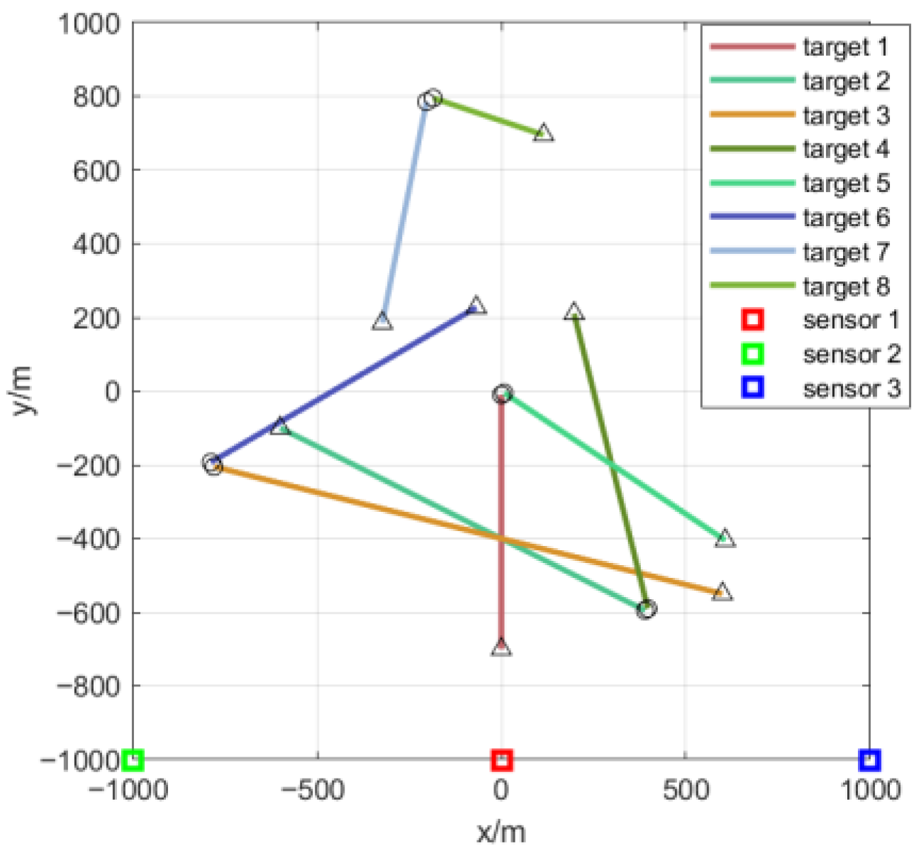
As shown in Figure 1, all targets move at the same speed along a straight path. The starting and finishing positions are shown by the circles and triangles, while the locations of all three sensors are shown by the squares. In the first scenario, each sensor has a detection range covering the entire area and a sampling rate of 1 Hz, and only monitors the position of targets.

The target state is denoted as $x_k={\left[p_{x,k},p_{y,k},{\dot{p}}_{x,k},{\dot{p}}_{y,k}\right]}^T$, where $p_{x/y,k}$ denotes the position and ${\dot{p}}_{x,k}$ denotes the velocity. The measurement from the sensor $s$ is denoted as $z_k^{(s)}={\left[z_{x,k}^{(s)},z_{y,k}^{(s)}\right]}^T$. $F_k$, $H_k$, $Q_k$, and $R_k$ are defined as

$$F_k=\left[\begin{array}{cc}{I}_2& \Delta I_2\\ 0_2& I_2\end{array}\right],Q_k={\sigma }_w^2\left[\begin{array}{cc}{\displaystyle \frac{{\Delta }^4}{4}}{I}_2& {\displaystyle \frac{{\Delta }^3}{2}}{I}_2\\ {\displaystyle \frac{{\Delta }^3}{2}}{I}_2& {\Delta }^2{I}_2\end{array}\right]$$

$$H_k=\left[\begin{array}{cc}{I}_2& 0_2\end{array}\right],R_k={\sigma }_{\epsilon }^2{I}_2$$

respectively, where $I_2=\left[\begin{array}{cc}1& 0\\ 0& 1\end{array}\right]$, $0_2=\left[\begin{array}{cc}0& 0\\ 0& 0\end{array}\right]$, $\Delta =1\mathrm{s}$, ${\sigma }_v=5{\mathrm{m}/\mathrm{s}}^2$, ${\sigma }_w=10\mathrm{m}$. The target survival probability and detection probability are $p_s=0.99$ and $p_D=0.98$, while the newborn targets follow an LMB distribution with four components. The clutter follows a Poisson distribution with ${\lambda }_c=30$.

Table 2. Target initial states and duration.

Target	Initial State	Duration (s)
1	${\left[0,0,0,-10\right]}^T$	$1~70$
2	${\left[400,-600,-10,5\right]}^T$	$1~100$
3	${\left[-800,-200,20,-5\right]}^T$	$1~70$
4	${\left[400,-600,-2.5,10\right]}^T$	$20~100$
5	${\left[0,0,7.5,-5\right]}^T$	$20~100$
6	${\left[-800,-200,12,7\right]}^T$	$40~100$
7	${\left[-200,800,-3,-15\right]}^T$	$60~100$
8	${\left[-200,800,15,-5\right]}^T$	$80~100$

shows the initial state and duration of each target, while the tracking performance is evaluated by the Optimal Sub-pattern Assignment (OSPA) distance [32] and the OSPA⁽²⁾ (OSPA-on-OSPA) distance [33]. The OSPA distance measures dissimilarity between two point sets, consisting of position and cardinality errors. A smaller value means better multi-target tracking performance, but it fails to reflect track label switching errors. Thus, the OSPA⁽²⁾ distance is included for comparison: it captures the overall error between true and estimated trajectory sets across multiple time steps, reflecting the effects of trajectory fragmentation and label switching, thereby more comprehensively evaluating multi-target tracking performance. All subsequent experimental results are the average values obtained from 100 Monte Carlo trials.

We conduct a comparison between the proposed MS-GLMB-S and three existing methods: the GLMB filter (SS-GLMB) [34], the centralized MS-GLMB filter (MS-GLMB), and the GLMB smoother (SS-GLMB-S). Since SS-GLMB and SS-GLMB-S are designed for single-sensor scenarios, we utilize measurements from sensor 1. It is worth noting that since the type and detection range of the three sensors are identical, selecting any one of them will not affect the experimental results. For MS-GLMB and MS-GLMB-S, we utilize measurements from all three sensors. Notably, the lag interval length of MS-GLMB-S is also set to 1 in the simulation.

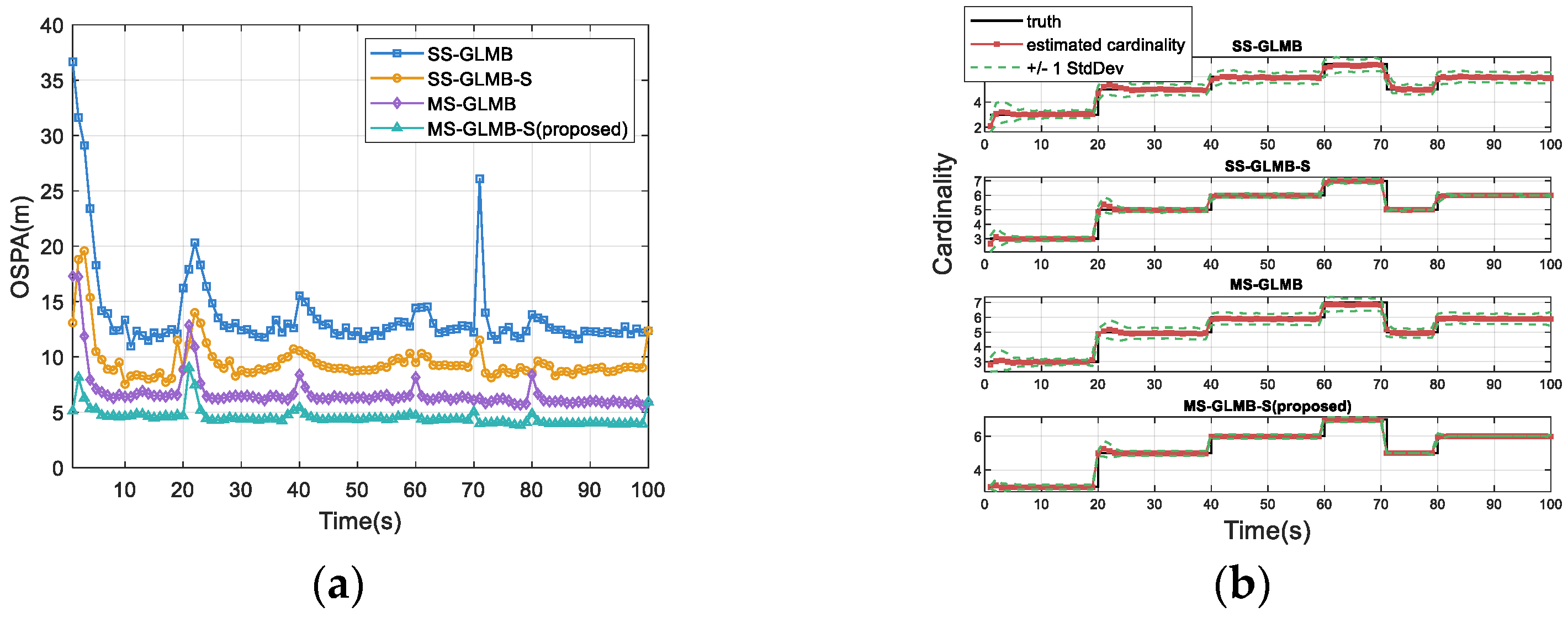
The OSPA distances and cardinality estimations corresponding to four methods are displayed in Figure 2a,b. It is evident that the proposed MS-GLMB-S significantly outperforms SS-GLMB, SS-GLMB-S, and MS-GLMB. This performance gain is attributed to the fact that MS-GLMB-S not only considers the measurements from multiple sensors, but also uses all the measurements within the lag interval to update the previous target state.

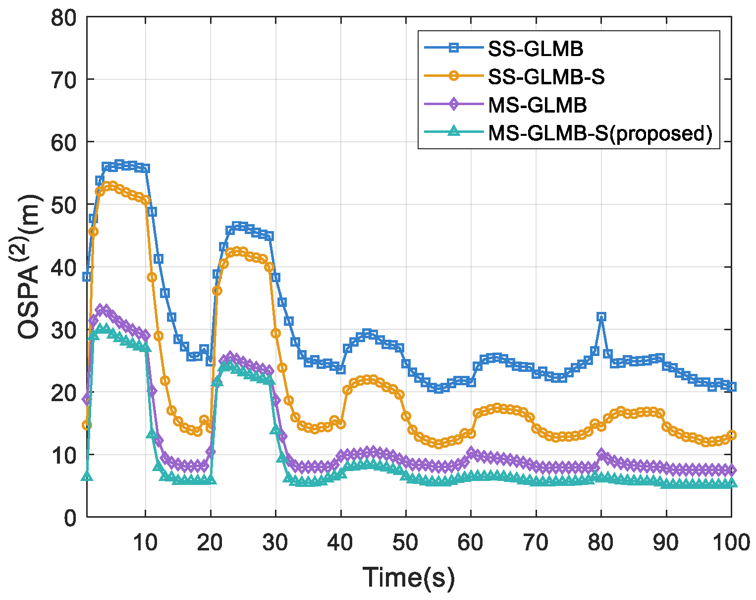
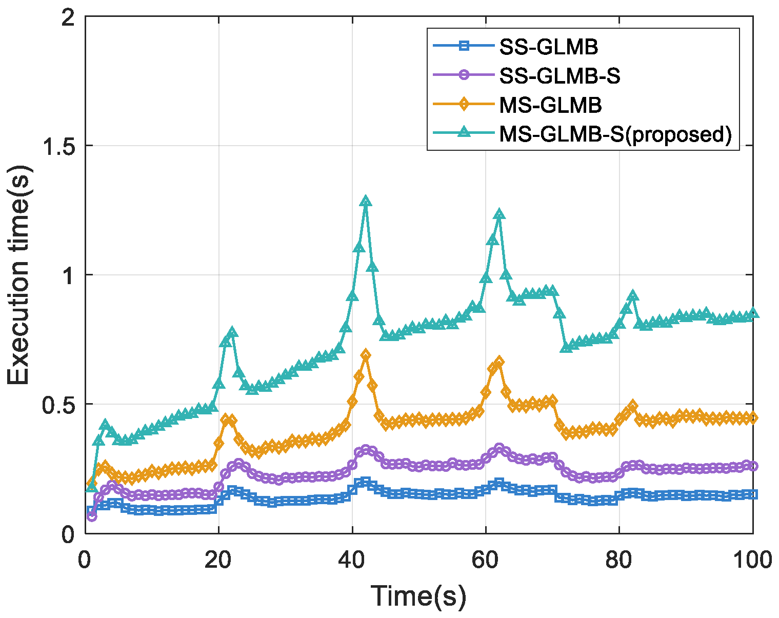
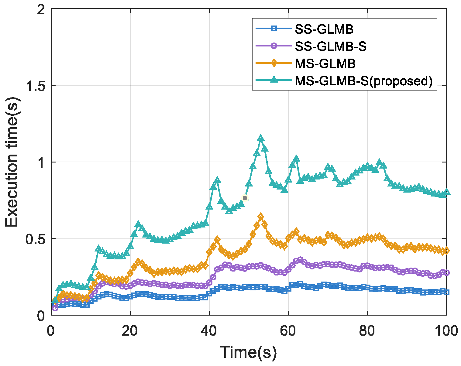
Figure 3 shows that the proposed MS-GLMB-S consistently achieves the smallest OSPA⁽²⁾ distance, which indicates that it has the highest tracking accuracy and effectively reduces the impact caused by track label switching. Figure 4 presents the per-frame runtime of the four methods. Of these methods, MS-GLMB-S exhibits the relatively longest average runtime, as it requires processing measurement data from each sensor within the lag interval.

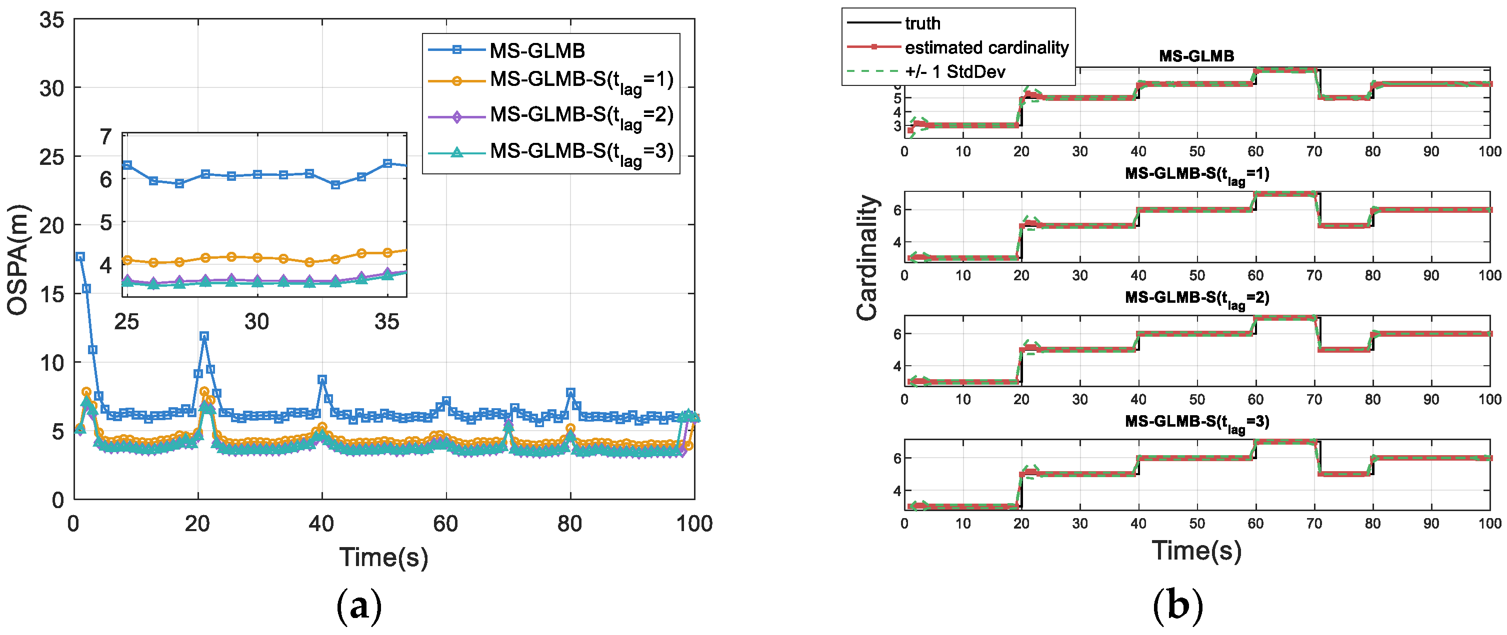
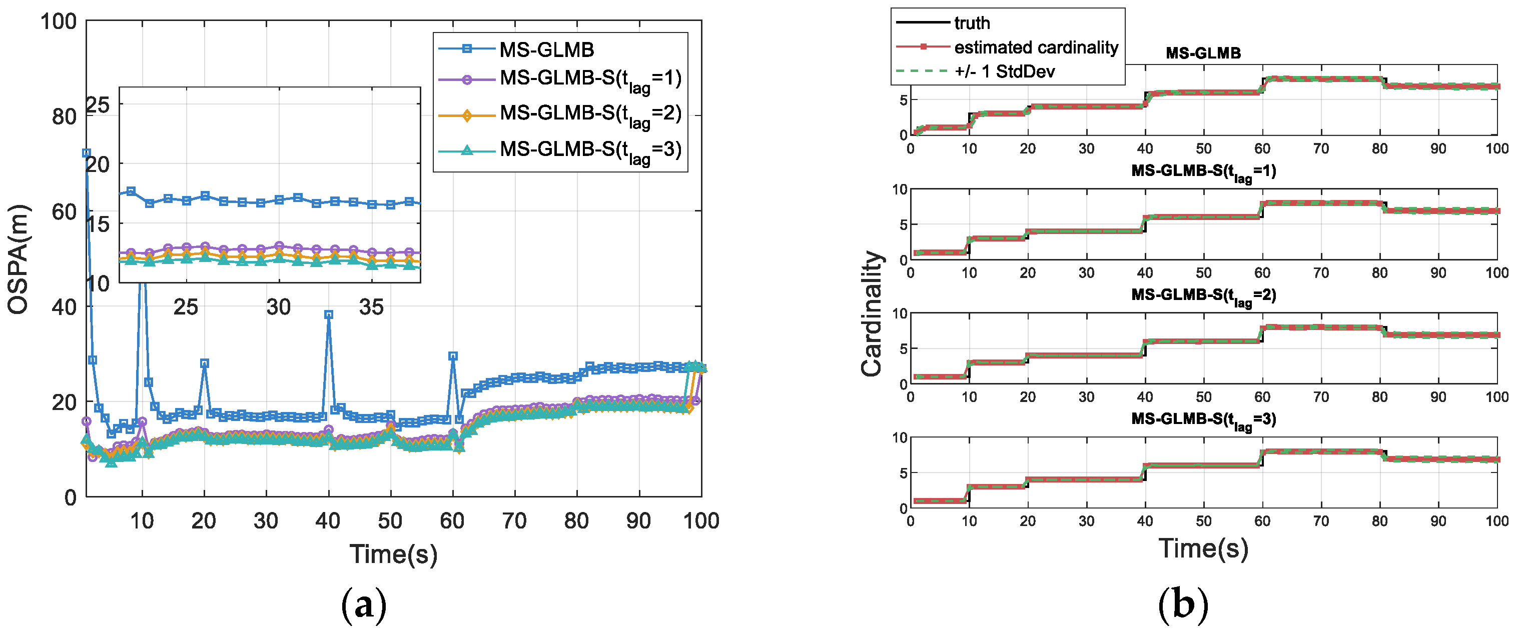
We further analyze the impact of varying lag intervals ($t_{lag}=\tau -k=0,1,2,3$) on the performance of MS-GLMB-S. When the lag interval length is set to 0, MS-GLMB-S reduces to the standard MS-GLMB filter. Figure 5a shows that the OSPA distance decreases with increasing lag interval length, indicating that the proposed MS-GLMB-S achieves superior tracking performance with a larger lag interval length. From Figure 5b, it is noticeable that the performance improvement of MS-GLMB-S with increasing lag steps is mainly reflected in the gradual reduction in the OSPA localization components, while the cardinality estimations are nearly identical and closely match the true value. This indicates that increasing the lag interval yields limited improvement in the estimation accuracy of the target number, but can further enhance the estimation accuracy of target positions.

Then we test the impacts of different numbers of sensors and lag intervals on the tracking accuracy and real-time performance of MS-GLMB-S, with the results presented in

Table 3. Average OSPA distance and average runtime of MS-GLMB-S under different lag intervals.

Number of Sensors	Lag (s)	OSPA Distance (m)	Runtime (s)
2	1	6.32	0.51
	2	5.63	0.73
	3	5.55	0.98
3	1	4.38	0.68
	2	3.91	0.95
	3	3.88	1.21

. Given the sensor sampling rate of 1 Hz, the tracking system is considered to have satisfactory real-time performance if the average runtime per frame is less than 1 s. As shown in Table 3, when the number of sensors is set to 2, the average runtime per frame is less than 1 s for lag interval lengths of 1, 2, and 3. However, as the lag interval length increases from 2 to 3, the average OSPA distance decreases by only 0.03 m, while the average runtime increases by 0.25 s. When the number of sensors is set to 3, the tracking accuracy is continuously improved. Nevertheless, when the lag interval length is 3, the average runtime per frame exceeds 1 s, leading to a significant degradation in real-time tracking performance.

In summary, increasing the lag interval length enhances the performance of MS-GLMB-S, but an excessively large lag is not advisable. This is because such a lag not only causes a significant growth in computational complexity and undermines real-time capability but also does not bring about any notable performance enhancement.

To evaluate the robustness of the proposed MS-GLMB-S, we compute OSPA and OSPA⁽²⁾ distance under varying $p_D$ and ${\lambda }_c$. The number of sensors is set to 3, and the lag interval length is set to 1. The results are derived from 100 Monte Carlo simulations. As shown in

Table 4. OSPA components and OSPA⁽²⁾ components of different $p_D$ and ${\lambda }_c$.

		$$\mathbf{Change}{\mathit{p}}_{\mathit{D}}({\mathit{\lambda }}_{\mathit{c}}=30)$$				$$\mathbf{Change}{\mathit{\lambda }}_{\mathit{c}}({\mathit{p}}_{\mathit{D}}=0.90)$$
		0.70	0.80	0.90	0.99	10	30	50	70
OSPA Dist (m)		11.99	7.39	6.38	4.30	5.95	6.29	6.59	7.92
OSPA Loc (m)		4.72	4.58	4.27	4.06	4.27	4.27	4.29	4.27
OSPA Card (m)		7.27	2.81	2.11	0.24	1.68	2.02	2.30	3.65
OSPA(2) Dist (m)		16.32	11.96	10.85	10.52	10.14	10.83	11.10	12.43
OSPA(2) Loc (m)		8.57	7.30	6.41	5.95	6.42	6.64	6.74	6.30
OSPA(2) Card (m)		7.75	4.66	4.44	4.57	3.72	4.19	4.36	6.13

, the impact of decreasing the $p_D$ on MS-GLMB-S performance is more notable than that of increasing ${\lambda }_c$; nevertheless, the OSPA distance and OSPA⁽²⁾ distance do not exhibit severe changes. Such results further confirm that MS-GLMB-S is robust to variations in both $p_D$ and ${\lambda }_c$.

5.2. Nonlinear

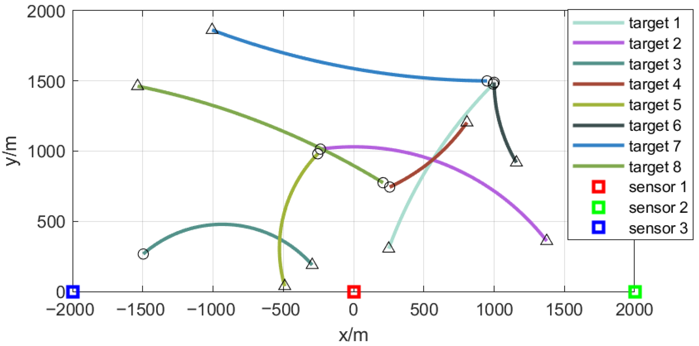
As shown in Figure 6, the starting and finishing positions are indicated by the circles and triangles, while the squares show the locations of all three sensors. Each target follows a nearly coordinated turn (NCT) model, with the state of interest represented by ${\left[x_k,{\omega }_k\right]}^T$, where $x_k={\left[p_{x,k},{\dot{p}}_{x,k},p_{y,k},{\dot{p}}_{y,k}\right]}^T$, and ${\omega }_k$ is the turning rate. The NCT model is expressed as follows.

$${\tilde{x}}_{k+1}=F\left({\omega }_k\right){\tilde{x}}_k+W_k$$

$${\omega }_{k+1}={\omega }_k+{\sigma }_u^2$$

where $F\left(\omega \right)=\left[\begin{array}{cccc}1& {\displaystyle \frac{\sin \omega \Delta }{\omega }}& 0& -{\displaystyle \frac{1-\cos \omega \Delta }{\omega }}\\ 0& c& 0& -\sin \omega \Delta \\ 0& {\displaystyle \frac{1-\cos \omega \Delta }{\omega }}& 1& {\displaystyle \frac{\sin \omega \Delta }{\omega }}\\ 0& \sin \omega \Delta & 0& \cos \omega \Delta \end{array}\right]$, $W_k={\sigma }_w^{2}G{G}^T$, $G=\left[\begin{array}{cc}{\displaystyle \frac{{\Delta }^2}{2}}& 0\\ \Delta & 0\\ 0& {\displaystyle \frac{{\Delta }^2}{2}}\\ 0& \Delta \end{array}\right]$.

We set ${\sigma }_v=5{\mathrm{m}/\mathrm{s}}^2$ and ${\sigma }_u=\pi /180\mathrm{rad}/\mathrm{s}$ as the turning rate noise. The target survival probability and detection probability are $p_s=0.99$ and $p_D=0.98$, while the newborn targets have the form of an LMB distribution with four components.

In the second scenario, each sensor still has a detection range covering the entire area and a sampling rate of 1 Hz, and monitors the range and azimuth of targets. Measurements from the sensor $s$ are noisy vectors of range and bearing $z_k^{(s)}={\left[r_k^{(s)},{\theta }_k^{(s)}\right]}^T$. $H^{(s)}$ for the sensors $s$ and $R$ are given as follows.

$$H^{(s)}\left(\cdot \right)=\left[\begin{array}{c}\sqrt{{\left(p_x-p_x^{(s)}\right)}^2+{\left(p_y-p_y^{(s)}\right)}^2}\\ \arctan \left(p_x-p_x^{(s)},p_y-p_y^{(s)}\right)\end{array}\right],R=\left[\begin{array}{cc}{\sigma }_r^2& 0\\ 0& {\sigma }_b^2\end{array}\right]$$

where $\left[p_x^{(s)},p_y^{(s)}\right]$ is the position of the sensor $s$, explicitly given by $\left[0,0\right]\mathrm{m}$, $\left[2000,0\right]\mathrm{m}$, and $\left[-2000,0\right]\mathrm{m}$. Range noise is ${\sigma }_r=5\mathrm{m}$ and bearing noise is ${\sigma }_b=\left(\pi /180\right)\mathrm{rad}$. The clutter follows a Poisson distribution with ${\lambda }_c=15$.

Table 5. Target initial states and duration.

Target	Initial State	Duration (s)
1	${\left[1000,-10,1500,-10,1/4\right]}^T$	$1~100$
2	${\left[-250,20,1000,3,-2/3\right]}^T$	$10~100$
3	${\left[-1500,11,250,10,-1\right]}^T$	$10~100$
4	${\left[250,11,750,5,1/2\right]}^T$	$20~80$
5	${\left[-250,-12,1000,-12,1\right]}^T$	$40~100$
6	${\left[1000,0,1500,-10,1/2\right]}^T$	$40~100$
7	${\left[1000,-50,1500,0,-1/2\right]}^T$	$60~100$
8	${\left[-250,-40,750,25,1/2\right]}^T$	$60~100$

illustrates the initial state and duration of each target.

We then show the comparison of the proposed MS-GLMB-S with SS-GLMB, MS-GLMB, and SS-GLMB-S in the second scenario. For SS-GLMB and SS-GLMB-S, we utilize measurements from sensor 1. It is also worth noting that although the sensor measurements in the second experiment differ from those in the first, the type and detection range of the three sensors are identical. Thus, selecting any one of them will not affect the experimental results. For MS-GLMB and MS-GLMB-S, we utilize measurements from all three sensors. All subsequent experimental results are the average values obtained from 100 Monte Carlo trials.

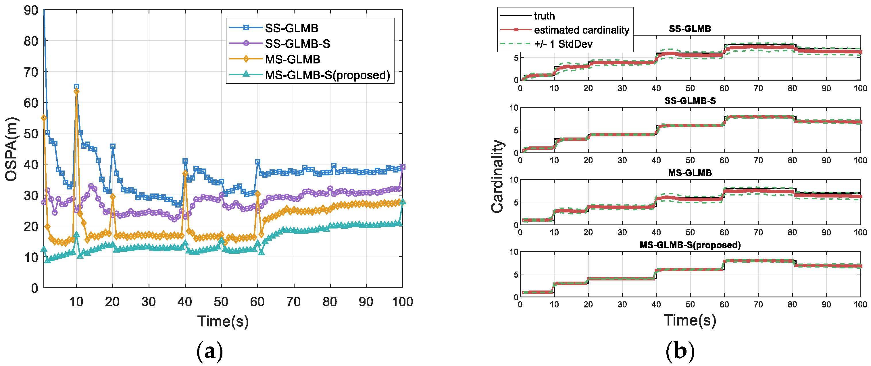
Figure 7a,b show the OSPA distance and the cardinality estimation of the four methods. It is clear that even as the cardinality estimations of SS-GLMB and SS-GLMB-S show significant deviations after 50 s, MS-GLMB-S still maintains a smaller OSPA distance and a more accurate cardinality estimation in comparison to the other three methods. This demonstrates that in nonlinear target motion scenarios, MS-GLMB-S provides significantly higher target state estimation accuracy than SS-GLMB, SS-GLMB-S, and MS-GLMB.

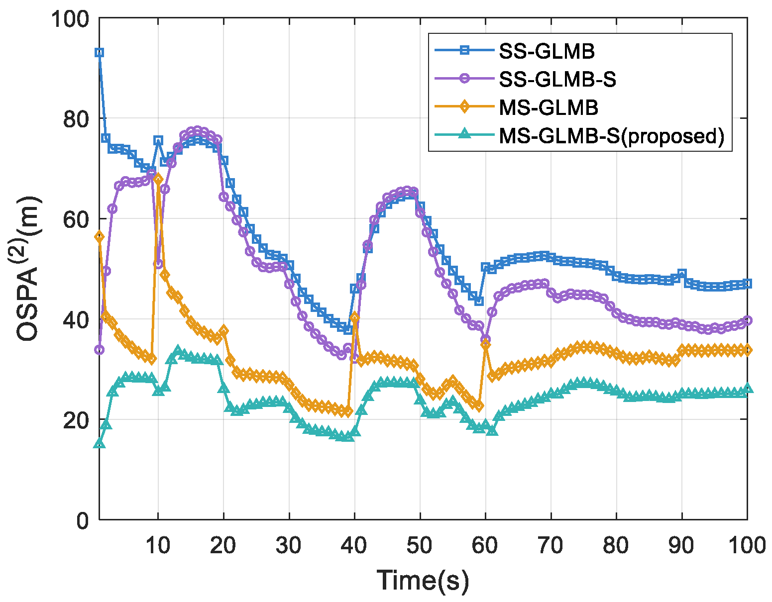
Figure 8 presents the OSPA⁽²⁾ distances for the four competing methods, with MS-GLMB-S demonstrating a smaller OSPA⁽²⁾ distance compared to the remaining three. This indicates that in nonlinear scenarios, the MS-GLMB-S algorithm achieves the optimal tracking accuracy and effectively reduces the impact of track label switching. Meanwhile, Figure 9 further shows that even in the context of more challenging nonlinear scenarios, the fluctuation range of the runtime curve of the MS-GLMB-S algorithm exhibits no significant difference compared with that in linear scenarios.

We then analyze the impact of varying lag intervals on the tracking accuracy and real-time performance of MS-GLMB-S. As illustrated in Figure 10 and

Table 6. Average OSPA distance and average runtime of MS-GLMB-S under different lag intervals.

Number of Sensors	Lag (s)	OSPA Distance (m)	Runtime (s)
2	1	16.79	0.55
	2	15.36	0.76
	3	15.11	0.95
3	1	14.35	0.62
	2	13.67	0.89
	3	13.38	1.15

, increasing the lag interval can enhance the performance of MS-GLMB-S; however, as discussed in Section 5.1, this lag interval length should not be excessively large.

Overall, the proposed MS-GLMB-S demonstrates robust applicability in scenarios with nonlinear target motion and nonlinear sensor measurements, achieving better tracking performance compared to SS-GLMB, SS-GLMB-S, and MS-GLMB.

6. Conclusions

The centralized multi-sensor GLMB smoother (MS-GLMB-S) proposed in this paper is based on the Bayesian forward–backward framework, which includes backward smoothing and forward filtering. In the forward filtering part, the filtering posterior density is generated by the centralized MS-GLMB filter. In the backward smoothing part, we derive expressions for the smoothing density and the simplified multi-sensor backward corrector in multi-sensor scenarios. With the filtering density and multi-sensor measurements within the lag interval, the weights of the GLMB components are adjusted to the corresponding smoothing weights. Subsequently, a suboptimal Gibbs sampling method for smoothing is introduced to truncate the GLMB smoothing density for efficient implementation of MS-GLMB-S, allowing different sensors to sample independently at different time steps within the lag interval. Additionally, the calculation of smoothing parameters in the linear Gaussian mixture model is detailed. In both linear and nonlinear simulation settings, the MS-GLMB-S has been shown to outperform SS-GLMB, MS-GLMB, and SS-GLMB-S.

Since MS-GLMB-S does not consider target birth and death during the smoothing process, cardinality estimation fluctuates significantly at these moments. Future improvements can incorporate target birth and death to refine the multi-sensor multi-target forward–backward smoothing framework and verify its effectiveness. In addition, the proposed MS-GLMB-S is currently only applicable to multi-sensor scenarios with centralized fusion; future work can further extend its application to multi-sensor scenarios based on distributed fusion.