Article

Forward and Backpropagation-Based Artificial Neural Network Modeling Method for Power Conversion System

1
Department of Electronic and Electrical Engineering, Keimyung University, Daegu 42601, Republic of Korea
2
Department of Electrical Engineering, Keimyung University, Daegu 42601, Republic of Korea
*
Author to whom correspondence should be addressed.
Electronics 2025, 14(23), 4718; https://doi.org/10.3390/electronics14234718
Submission received: 10 October 2025 / Revised: 27 November 2025 / Accepted: 28 November 2025 / Published: 29 November 2025
(This article belongs to the Section Systems & Control Engineering)

Abstract

The PCS controls and converts the flow of electrical power. Generally, it uses sensors to measure voltage and current. However, these sensors require careful tuning across their entire operating range. Additionally, they lead to increased system complexity, greater physical volume, and higher maintenance costs. Therefore, to address these challenges, this paper proposes a forward and backpropagation-based ANN modeling method for PCS. The proposed ANN modeling method is trained using forward and backpropagation to learn the nonlinear relationships between system inputs and outputs. Through this training process, the proposed ANN modeling method can accurately predict system variables without sensors or mathematical modeling. Furthermore, by eliminating the need for sensors, the system structure can be simplified, and the overall cost significantly reduced. This paper focuses on mathematically deriving and implementing a forward and backpropagation-based ANN modeling method, and it verifies its prediction performance using a series-parallel resistor circuit. The validity of the proposed ANN modeling method is verified by simulation and experimental results.

1. Introduction

A power conversion system (PCS) controls and converts the flow of electrical power, such as voltage, current, and frequency. Representative PCSs include inverters that convert DC power into AC power, converters that step up or step down input DC power, and rectifiers that convert AC power into DC power. These PCSs control electrical characteristics to convert power suitable for the load and are widely applied in various applications such as household electronics, electric vehicles, railways, renewable energy systems, and industrial power equipment [1,2,3,4].
Generally, PCSs aim to minimize energy loss and increase efficiency by using passive elements such as inductors, capacitors, and switches. In addition, stable operation, high precision, and fast response are required under various driving conditions to improve the stability and reliability of the system [5,6,7]. However, the performance of these components is not constant and may degrade over time or under changing environmental conditions. For instance, inductors can undergo magnetic saturation, switching elements are sensitive to changes in on-resistance, and capacitors and resistors are influenced by equivalent series resistance (ESR) and temperature coefficients, respectively. These factors result in a time-varying and nonlinear system behavior, making accurate modeling and analysis challenging.
In PCS, various types of sensors such as shunts, hall-effect sensors, and fluxgate sensors are used to measure voltage and current in real-time. These sensors rapidly measure the electrical state of the circuit and provide real-time data. However, these sensors require careful tuning and calibration process over their operating range, and measurement errors may occur due to noise or external disturbances. Furthermore, since most of them output analog signals, an analog-to-digital converter (ADC) is required to convert analog signals into digital signals. In PCS, high-speed sampling is required, necessitating the use of external ADCs. It leads to increased system complexity, physical volume, and higher maintenance costs [8,9,10].
Recently, to address these challenges of sensor measurement, artificial intelligence (AI) technologies have begun to be applied in the PCS [11,12,13]. These technologies, such as machine learning, deep learning, and artificial neural network (ANN), can learn system operation characteristics through input and output variables even without mathematical modeling of the system. In addition, they can predict the voltage and current conditions without sensors. Among them, ANN is widely used in the PCS due to its relatively simple structure and capability to learn complex nonlinear relationships. It consists of an input layer, hidden layers, and an output layer. ANN learns complex nonlinear relationships by calculating output values using forward propagation and updating the weights and biases based on the error using backpropagation. These ANNs have already been widely applied in hardware applications within power systems, such as temperature estimation, fault diagnosis, and condition monitoring [14,15,16,17]. However, there are relatively few studies that focus on software applications aiming to accurately predict electrical operations such as voltage and current inside a circuit.
Meanwhile, various AI approaches such as black-box neural networks, physics-informed neural networks, and hybrid AI-analytical models have been utilized in PCS [18,19,20]. These methods have the advantage of effectively considering nonlinear and dynamic characteristics. However, most of these methods assume the availability of accurate analytical models or focus on improving control performance and efficiency. In particular, most ANN-based PCS studies tend to rely on commercial software frameworks. Since the forward and backpropagation processes are implemented using toolboxes and training modules provided by such software, the detailed derivation and implementation procedures for the neurons in each layer, forward propagation, and backpropagation processes are usually not addressed. As a result, it is difficult to directly implement or analyze the ANN training process based on forward and backpropagation, as well as to modify or extend the training process according to the circuit characteristics.
Therefore, to accurately predict the electrical operations of PCS, this paper proposes a forward and backward propagation-based ANN modeling method for PCS. The proposed ANN modeling method employs the forward propagation to establish the input-output relationship using weights and biases, and the backpropagation to update the weights and biases by minimizing the error between the neural network outputs and the target outputs. Through this training process, the proposed ANN modeling method can accurately predict system variables without sensors or mathematical modeling, and maintain high prediction accuracy even under varying load conditions and external disturbances. Furthermore, by eliminating the need for sensors, the system structure can be simplified and the overall cost significantly reduced. This paper focuses on deriving and implementing the forward and backpropagation for predicting circuit voltages and currents rather than proposing a new ANN architecture or training method. The validity of the proposed ANN modeling method is verified by simulation and experimental results.

2. Power Conversion Systems Modeling

2.1. Circuit Configuration and Operating Characteristics

Figure 1 shows a series-parallel resistor circuit composed of a DC voltage Vin and four 60 Ω resistors. Each resistor is arranged in a combination of series and parallel connections, and the input current flows are distributed along each current path. The circuit in Figure 1 clearly defines the node voltages and branch currents, allowing for intuitive verification of the agreement between theoretical and measured values. Furthermore, it reproduces the resistive distribution characteristics of the PCS, making it suitable for verifying the validity of the ANN. The circuit is theoretically interpreted as a linear system, and the voltage and current of each resistor are determined based on Ohm’s Law, Kirchhoff’s Current Law (KCL), and Kirchhoff’s Voltage Law (KVL). The laws are expressed in (1), (2), and (3).
V i = I i R i       i = 1 ,   2 ,   3 ,   4 .
I t o t a l = i = 1 n I i = V i n R e q     R e q = i = 1 n R i     n = 1 ,   2 ,   3 ,   4 .
i = 1 n V i = V i n       n = 1 ,   23 ,   4 ,         V 23 = V 2 = V 3 .
In theory, the voltage and current of each resistor can be easily calculated based on these laws. However, in the actual implementation environment, the circuit does not operate linearly due to various factors. Most resistors have the characteristic that the resistance value increases or decreases depending on the temperature, and in high current situations, the resistance value may change in real time due to heat generation. In addition, due to manufacturing tolerances, the actual resistance values may have a certain degree of difference from the specified value, and long-term usage can lead to physical degradation of material properties. Furthermore, interference from the measuring equipment or the surrounding environment may distort the output value. As a result, these factors limit the ability to predict the output characteristics from a simple theoretical model, and the actual circuit behaves more like a time-varying and uncertain system than an ideal linear system.
Since the series-parallel resistor circuit has a simple structure and a theoretically simple interpretable characteristic, this circuit is used as a verification circuit for validating the proposed ANN modeling method. The predictive performance of an ANN can be evaluated by comparing the differences between the theoretical model and actual data using the series-parallel resistor circuit. This paper focuses on the validity and implementation of the forward and backpropagation-based ANN modeling method and limits the verification variables to V4 and I4.

2.2. Necessity of Predictive Modeling

PCS may operate differently from analytical results due to various factors, and these factors create a complex environment characterized by nonlinearity, load conditions, and external disturbances. Generally, mathematical modeling methods are used for circuit analysis of power conversion systems, and they have the advantages of a simple structure and intuitive calculations. However, their accuracy tends to decrease when the load conditions vary over time. It is difficult to reflect actual component values caused by factors such as temperature, time, and disturbances in real time. Most of the subtle effects, such as noise, measurement errors, and losses, are often neglected in the analysis model. In addition, as the circuit structure becomes more complex or the number of components increases, mathematical modeling becomes exponentially more complex.
These limitations can cause errors between theory and actual practice, even in simple circuits, and they can lead to decreased prediction accuracy in complex PCS environments. Therefore, the need for a prediction method that can flexibly respond to parameter variations and external disturbances and train actual operating characteristics without mathematical modeling is increasing.

3. Artificial Neural Network Modeling Method

3.1. Structure of Proposed Artificial Neural Network

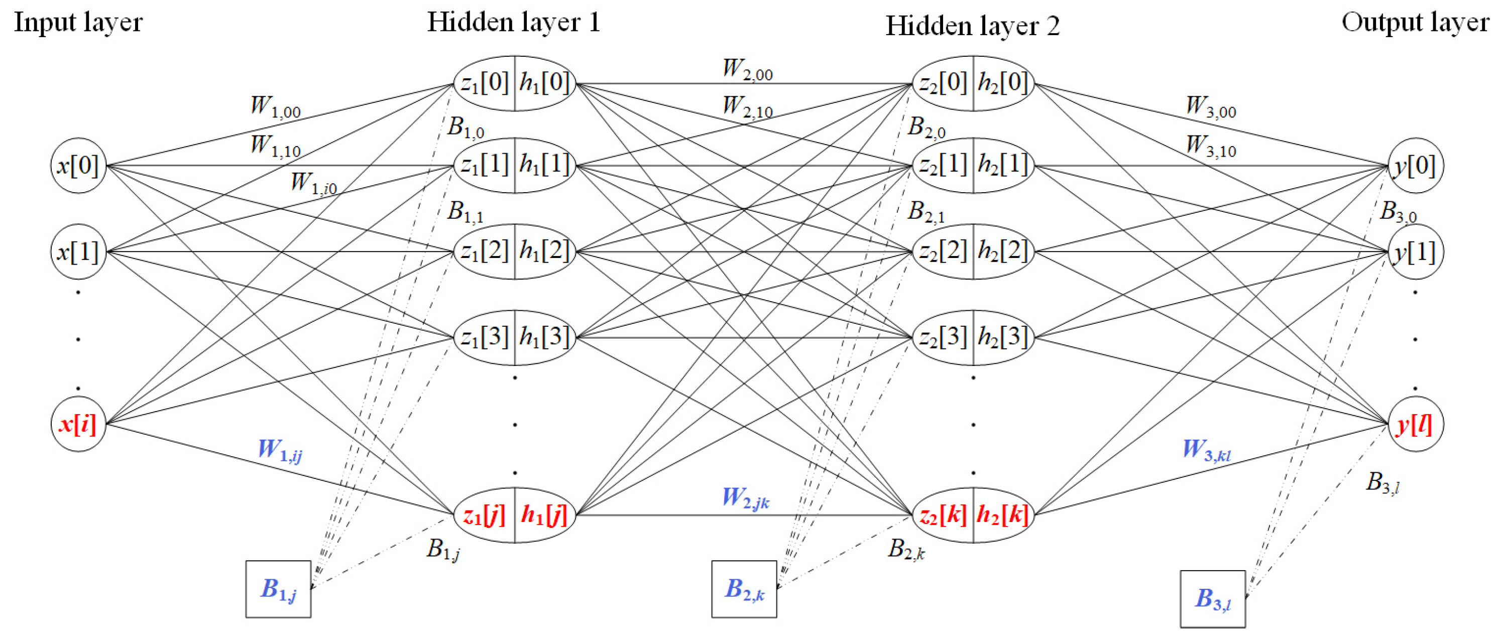
Figure 2 shows the structure of the proposed ANN, which applies a multilayer perceptron. The proposed ANN consists of an input layer, two hidden layers, and an output layer. The number of hidden layers was selected by considering system complexity, data volume, and training accuracy requirements.
The input layer receives the main input values (x[i]) of the PCS and passes them to the hidden layer. The x[i] can be composed of various types such as the system’s input voltage, input current, load conditions, and current changes. These values are transferred to the output layer through the hidden layer. The output values (y[l]) can be composed of various types such as the system’s output voltage, output current, speed, position, and control input. The clearer the relationship between the input and output values, the higher the training efficiency and accuracy. Therefore, the selection of input and output values is important.
The proposed ANN is designed to learn the complex nonlinear relationships of the PCS and can respond to various parameter variations, load condition changes. The proposed ANN is trained through forward propagation and backpropagation, where the weights and biases are optimized to minimize the error between the targets and the outputs of the ANN.

3.2. Forward Propagation Modeling

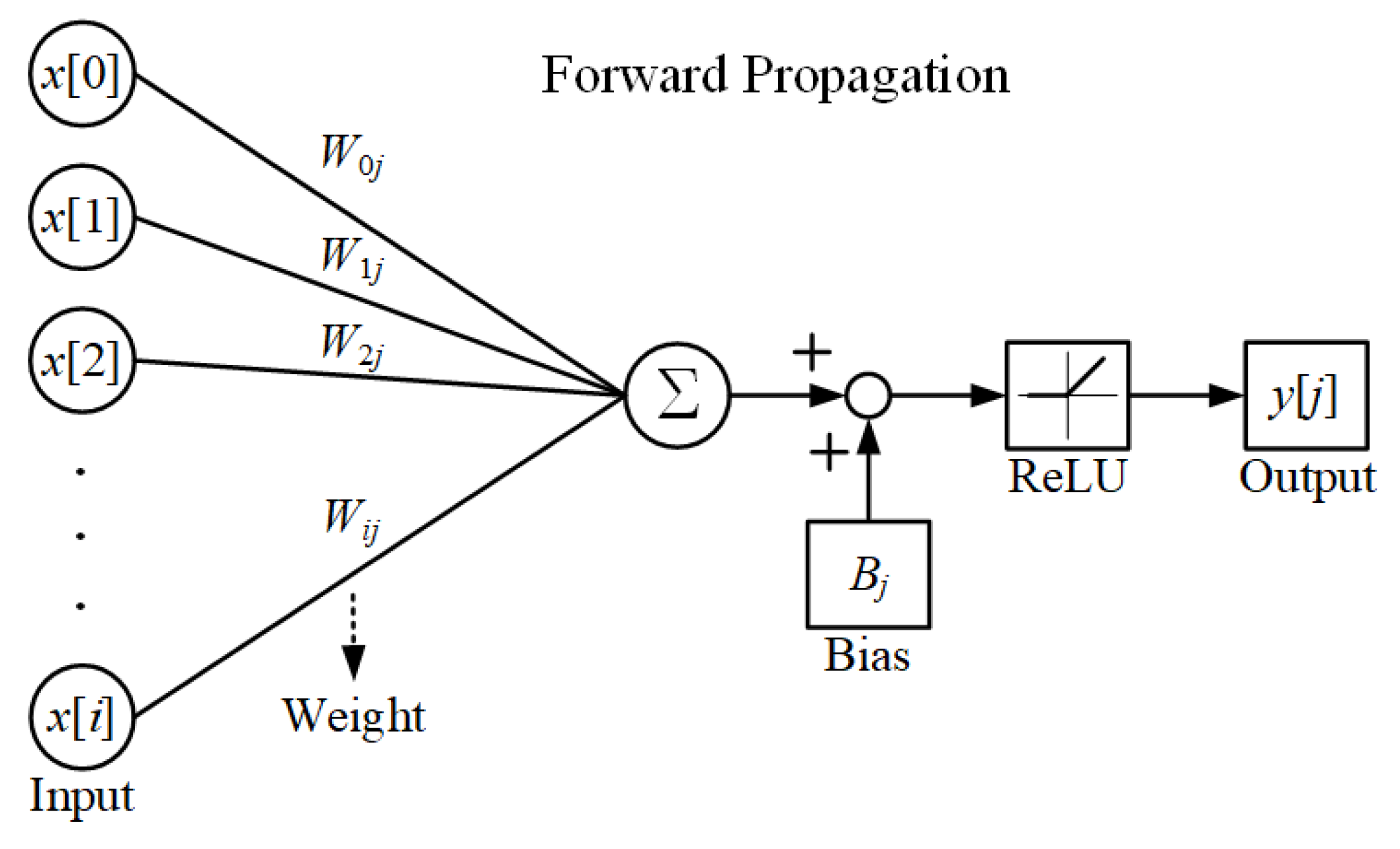
Figure 3 shows the forward propagation of the ANN in each layer. The forward propagation process determines the output of the ANN through the input layer, hidden layers, and output layer.
Initially, input values are provided to the network, after which they undergo a series of calculations involving weights and biases. Subsequently, a nonlinear activation function is applied to determine the output value. The output value is transferred to the subsequent layer and then serves as the input value for the subsequent layer. The nonlinear activation functions commonly used include the sigmoid function, hyperbolic tangent (Tanh), and rectified linear unit (ReLU). In this paper, the ReLU function, which offers high computational efficiency and a simple structure, is adopted. The ReLU function is defined as in (4) [21,22,23].
ReLU x = x         x > 0 0         x 0 .
The proposed ANN structure, as shown in Figure 3, consists of an input layer, two hidden layers, and an output layer, and the forward propagation process of each layer is expressed as in (5).
z 1 j = i W 1 , i j x i + B 1 , j ,     h 1 j = ReLU z 1 j , z 2 k = j W 2 , j k h 1 j + B 2 , k ,     h 2 k = ReLU z 2 k , y l = k W 3 , k l h 2 k + B 3 , l ,
where z1[j] is the input value to the activation function of the first hidden layer, h1[j] is the output of the first hidden layer. Similarly, W2,jk, B2,k, z2[k], and h2[k] represent the corresponding weights, biases, input value of the activation function, and outputs of the second hidden layer, respectively. Finally, W3,kl and B3,l are the weight and bias connecting the second hidden layer to the output layer, and y[l] is the final output of the ANN.

3.3. Backpropagation Modeling

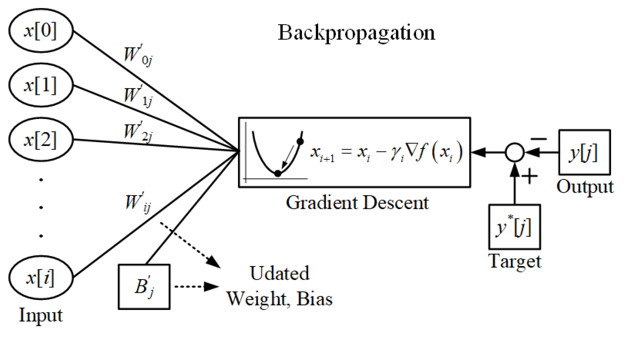
Figure 4 shows the backpropagation of the ANN in each layer. The backpropagation process updates the weights and biases to the optimal values when an error occurs between the target value and the output of the ANN, aiming to minimize the error to zero.
Implementing an ANN requires detailed derivations of backpropagation. However, existing research rarely explores this process. To address this issue, this paper presents the full derivation process based on standard backpropagation. This derivation process is based on the conventional backpropagation process and is adapted to the MLP structure used in this paper [24,25,26].
Typically, gradient descent based on a loss function is used to update the weights and biases. Gradient descent is an optimization technique that finds the minimum of a function by continuously updating the coefficients in the direction that reduces the function value based on its gradient. Gradient descent is expressed as in (6) and calculates the next location from the current location for the function to be optimized.
x i + 1 = x i γ i f x i ,
where f(xi) is the optimization function, xi is the current location, xi+1 is the next location to be moved, and γi is a parameter that controls the distance to be moved.
When applied to ANN, the f(xi) is set as a loss function, and xi and xi+1 are set as weights and biases. A loss function measures the difference between the target value and the output value, serving as an indicator of the model’s prediction accuracy. The loss functions used in regression problems are typically mean squared error (MSE) and mean absolute error (MAE) functions. The MSE function is commonly used due to its effectiveness in minimizing the error between the target and output values [27,28,29]. The loss function used in the proposed ANN is expressed as in (7), and the weight and bias updates using gradient descent are expressed as in (8).
MSE = E t o t a l = 1 2 y l y l 2 ,
W n e w = W o l d η E t o t a l W ,     B n e w = B o l d η E t o t a l B ,
where Etotal is the loss function, η is the learning rate, and y*[l] is the target value. In the gradient descent method, the gradient and η determine the update direction. If the η and gradient are too small, the training process becomes slow, while overly large values can cause divergence. Therefore, appropriate settings for the gradient and η are necessary.
Since the backpropagation proceeds in the opposite direction to the forward propagation, the weights and biases between the output layer and the second hidden layer are updated first by applying gradient descent. Applying gradient descent to update the weights and biases between the output layer and the second hidden layer, the result is expressed as in (9).
W 3 , k l _ n e w = W 3 , k l _ o l d η E t o t a l W 3 , k l ,     B 3 , l _ n e w = B 3 , l _ o l d η E t o t a l B 3 , 0 .
For example, the update method of the weight (W3,00), which connects the first neuron (h2[0]) of the second hidden layer and the output neuron (y[0]) of the output layer, is expressed as in (10). For convenience, the partial derivative of Etotal with respect to the W3,00 is calculated using the chain rule.
W 3 , 00 _ n e w = W 3 , 00 _ o l d η E t o t a l y 0 × y 0 W 3 , 00 .
By applying the chain rule, the partial derivative of the Etotal with respect to the W3,00 is calculated as in (11) and rewritten as in (12).
E t o t a l y 0 = d d y 0 1 2 y 0 y 0 2 = y 0 y 0 , y 0 W 3 , 00 = d d W 3 , 00 h 2 0 × W 3 , 00 + h 2 1 × W 3 , 10 + + h 2 k × W 3 , k 0 + B 3 , 0 = h 2 0 .
E t o t a l W 3 , 00 = y 0 y 0 × h 2 0 .
The update method of the bias (B3,0), which connects the y[0], is expressed as in (13), and it is similarly calculated using the chain rule.
B 3 , 0 _ n e w = B 3 , 0 _ o l d η E t o t a l y 0 × y 0 B 3 , 0 .
By applying the chain rule, the partial derivative of the Etotal with respect to the B3,0 is calculated as in (14) and rewritten as in (15).
E t o t a l y 0 = d d y 0 1 2 y 0 y 0 2 = y 0 y 0 , y 0 B 3 , 0 = d d B 3 , 0 h 2 0 × W 3 , 00 + h 2 1 × W 3 , 10 + + h 2 k × W 3 , k 0 + B 3 , 0 = 1 .
E t o t a l B 3 , 0 = y 0 y 0 .
The updated W3,00 and B3,0 through the above process are summarized as in (16).
W 3 , 00 _ n e w = W 3 , 00 _ o l d η y 0 y 0 × h 2 0 , B 3 , 0 _ n e w = B 3 , 0 _ o l d η y 0 y 0 .
Similarly, the other weights W3,01, W3,02, …, W3,kl and biases B3,1, B3,2, …, B3,l can also be updated using the same approach.
Next, applying gradient descent to update the weights and biases between the first hidden layer and the second hidden layer, the result is expressed as in (17).
W 2 , j k _ n e w = W 2 , j k _ o l d η E t o t a l W 2 , j k ,     B 2 , k _ n e w = B 2 , k _ o l d η E t o t a l B 2 , k .
For example, the update method of the weight (W2,00), which connects the first neuron (h1[0]) of the first hidden layer and the h2[0], is expressed as in (18), and it is similarly calculated using the chain rule.
W 2 , 00 _ n e w = W 2 , 00 _ o l d η E t o t a l y 0 × y 0 h 2 0 × h 2 0 z 2 0 × z 2 0 W 2 , 00 .
By applying the chain rule, the partial derivative of the Etotal with respect to the W2,00 is calculated as in (19) and rewritten as in (20).
E t o t a l y 0 = d d y 0 1 2 y 0 y 0 2 = y 0 y 0 , y 0 h 2 0 = d d h 2 0 h 2 0 × W 3 , 00 + h 2 1 × W 3 , 10 + + h 2 k × W 3 , k 0 + B 3 , 0 = W 3 , 00 , h 2 0 z 2 0 = d d z 2 0 ReLU z 2 0 = ReLU z 2 0 , z 2 0 W 2 , 00 = d d W 2 , 00 h 1 0 × W 2 , 00 + h 1 1 × W 2 , 10 + + h 1 j × W 2 , j 0 + B 2 , 0 = h 1 0 .
E t o t a l W 2 , 00 = y 0 y 0 × W 3 , 00 × ReLU z 2 0 × h 1 0 .
The update method of the bias (B2,0), which connects the h2[0], is expressed as in (21), and it is similarly calculated using the chain rule.
B 2 , 0 _ n e w = B 2 , 0 _ o l d η E t o t a l y 0 × y 0 h 2 0 × h 2 0 z 2 0 × z 2 0 B 2 , 0 .
By applying the chain rule, the partial derivative of the Etotal with respect to the B2,0 is calculated as in (22) and rewritten as in (23).
E t o t a l y 0 = d d y 0 1 2 y 0 y 0 2 = y 0 y 0 , y 0 h 2 0 = d d h 2 0 h 2 0 × W 3 , 00 + h 2 1 × W 3 , 10 + + h 2 k × W 3 , k 0 + B 3 , 0 = W 3 , 00 , h 2 0 z 2 0 = d d z 2 0 ReLU z 2 0 = ReLU z 2 0 , z 2 0 B 0 2 = d d B 2 , 0 h 1 0 × W 2 , 00 + h 1 1 × W 2 , 10 + + h 1 j × W 2 , j 0 + B 2 , 0 = 1 .
E t o t a l B 2 , 0 = y 0 y 0 × W 3 , 00 × ReLU z 2 0 .
The updated W2,00 and B2,0 through the above process are summarized as in (24).
W 2 , 00 _ n e w = W 2 , 00 _ o l d η y 0 y 0 × W 3 , 00 × ReLU z 2 0 × h 1 0 , B 2 , 0 _ n e w = B 2 , 0 _ o l d η y 0 y 0 × W 3 , 00 × ReLU z 2 0 .
Similarly, the other weights W2,01, W2,02, …, W2,jk and biases B2,1, B2,2, …, B2,k can also be updated using the same approach.
Finally, applying gradient descent to update the weights and biases between the input layer and hidden layer and the first hidden layer, the result is expressed as in (25).
W 1 , i j _ n e w = W 1 , i j _ o l d η E t o t a l W 1 , i j ,     B 1 , j _ n e w = B 1 , j _ o l d η E t o t a l B 1 , j .
For example, the update method of the weight (W1,00), which connects the first neuron (x[0]) of the input layer and the h1[0], is expressed as in (26), and it is calculated using the chain rule.
W 1 , 00 _ n e w = W 1 , 00 _ o l d η E t o t a l y 0 × y 0 h 2 0 × h 2 0 z 2 0 × z 2 0 h 1 0 × h 1 0 z 1 0 × z 1 0 W 1 , 00 .
By applying the chain rule, the partial derivative of the Etotal with respect to the W1,00 is calculated as in (27) and rewritten as in (28).
E t o t a l y 0 = d d y 0 1 2 y 0 y 0 2 = y 0 y 0 , y 0 h 2 0 = d d h 2 0 h 2 0 × W 3 , 00 + h 2 1 × W 3 , 10 + + h 2 k × W 3 , k 0 + B 3 , 0 = W 3 , 00 , h 2 0 z 2 0 = d d z 2 0 ReLU z 2 0 = ReLU z 2 0 , z 2 0 h 1 0 = d d h 1 0 h 1 0 × W 2 , 00 + h 1 1 × W 2 , 10 + + h 1 j × W 2 , j 0 + B 2 , 0 = W 2 , 00 , h 1 0 z 1 0 = d d z 1 0 ReLU z 1 0 = ReLU z 1 0 , z 1 0 W 1 , 00 = d d W 1 , 00 x 0 × W 1 , 00 + x 1 × W 1 , 10 + + x i × W 1 , i 0 + B 1 , 0 = x 0 .
E t o t a l W 1 , 00 = y 0 y 0 × W 3 , 00 × ReLU z 2 0 × W 2 , 00 × ReLU z 1 0 × x 0 .
The update method of the bias B1,0, which connects the h1[0], is expressed as in (29), and it is similarly calculated using the chain rule.
B 1 , 0 _ n e w = B 1 , 0 _ o l d η E t o t a l y 0 × y 0 h 2 0 × h 2 0 z 2 0 × z 2 0 h 1 0 × h 1 0 z 1 0 × z 1 0 B 1 , 0 .
By applying the chain rule, the partial derivative of the Etotal with respect to the B1,0 is calculated as in (30) and rewritten as in (31).
E t o t a l y 0 = d d y 0 1 2 y 0 y 0 2 = y 0 y 0 , y 0 h 2 0 = d d h 2 0 h 2 0 × W 3 , 00 + h 2 1 × W 3 , 10 + + h 2 k × W 3 , k 0 + B 3 , 0 = W 3 , 00 , h 2 0 z 2 0 = d d z 2 0 ReLU z 2 0 = ReLU z 2 0 , z 2 0 h 1 0 = d d h 1 0 h 1 0 × W 2 , 00 + h 1 1 × W 2 , 10 + + h 1 j × W 2 , j 0 + B 2 , 0 = W 2 , 00 , h 1 0 z 1 0 = d d z 1 0 ReLU z 1 0 = ReLU z 1 0 , z 1 0 B 1 , 0 = d d B 1 , 0 x 0 × W 1 , 00 + x 1 × W 1 , 10 + + x i × W 1 , i 0 + B 1 , 0 = 1 .
E t o t a l B 1 , 0 = y 0 y 0 × W 3 , 00 × ReLU z 2 0 × W 2 , 00 × ReLU z 1 0 .
The updated W1,00 and B1,0 through the above process are summarized as in (32).
W 1 , 00 _ n e w = W 1 , 00 _ o l d η y 0 y 0 × W 3 , 00 × ReLU z 2 0 × W 2 , 00 × ReLU z 1 0 × x 0 , B 1 , 0 _ n e w = B 1 , 0 _ o l d η y 0 y 0 × W 3 , 00 × ReLU z 2 0 × W 2 , 00 × ReLU z 1 0 × 1 .
Similarly, the other weights W1,01, W1,02, …, W1,ij and biases B1,1, B1,2, …, B1,j can also be updated using the same approach.

3.4. Overall Training Process

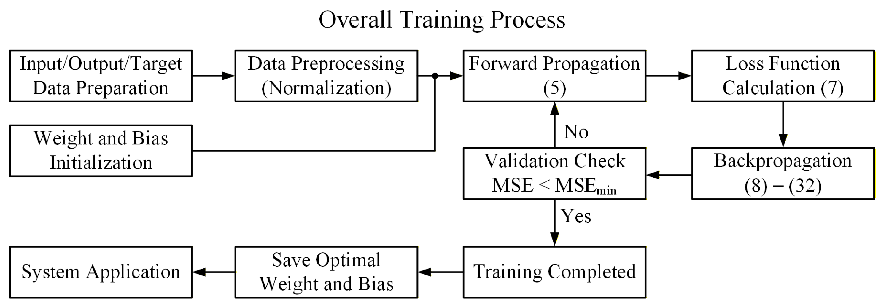
Figure 5 shows the overall training process of the proposed ANN. The overall training process is based on forward and backpropagation, where the weights and biases are updated iteratively to achieve optimization.
In the training process, the loss function is used to evaluate the prediction accuracy of the current model, and training is performed based on the error between the target value and the output value of the ANN.
The overall training process consists of the following:
  • Data preprocessing:
The input and target values of the ANN are scaled to a specific range through a preprocessing process such as normalization. Normalization can prevent sharp gradient changes in the loss function and enhance the training stability and speed. In addition, it can solve the local minimum phenomenon, which stops training at a local minimum rather than the global minimum. For example, scaling input voltage, current, and load conditions between 0 and 1 improve training stability.
2.
Weight and bias initialization:
All weights and biases are generally set to initial values and gradually adjusted through training. They should be initialized with random values. If all weights and biases are zero or have the identical values, each neuron will produce the identical output through forward propagation and have the identical gradients during the backpropagation process. As a result, all neurons will behave identically as one neuron, making it difficult to learn effectively.
3.
Forward propagation:
Once the normalized input values are applied to the input layer, it passes through the input layer, hidden layer, and output layer to determine the final output value of the ANN. Calculations are performed using the weights and biases, and nonlinear activation functions are applied to learn the nonlinearity of the system. In the case of PCSs, which are treated as regression problems, the nonlinear activation function is not applied to the output layer.
4.
Loss function calculation:
The error between the target value and the output obtained through forward propagation is calculated using the loss function. The proposed ANN uses the MSE function, which calculates the overall prediction accuracy by squaring the error of each sample and taking the average.
5.
Backpropagation:
If an error occurs between the target value and the output, the backpropagation process is performed using the gradient descent method based on the loss function. The error in each layer is calculated through the chain rule, and the weights and biases are updated through the chain rule. An excessively large η can cause divergence, and an excessively small η can slow down the convergence speed. Therefore, the η should be set appropriately.
6.
Iterative training and termination condition setting:
The forward and backpropagation processes are iterated for all data. One full cycle of training is referred to as an epoch, and when iterative training is completed for the set number of epochs, the average loss value or accuracy is evaluated. Training is terminated when the conditions are satisfied.
7.
Training completion and application.
Once training is completed, the optimal weights and biases are saved. The learned ANN can be used to infer outputs from new input values and be applied to various control parameters in PCS.
The training process of the proposed ANN can flexibly respond to the nonlinear characteristics of the PCS and the load and parameter variations over time. In addition, it can achieve high prediction accuracy and robust control performance through iterative training and can be applied to various control methods.

4. Simulation Results

The proposed forward and backpropagation-based ANN modeling method is verified for validity using PSIM simulation software, and the parameters used in the simulation are as shown in Table 1. i, j, k, and l were selected by comprehensively considering input and output variables, error convergence rate, and training speed. η was determined through experimental tuning within a stable range to prevent divergence and ensure stable convergence. In addition, the series-parallel resistor circuit, as shown in Figure 2, is used as a verification circuit for the proposed ANN modeling method. The input values of the ANN are set as the input voltage of the resistor circuit (Vin), the current flowing in the resistor (I1, I2, I3), and the voltage of the resistor (V1, V3). The target output values of the ANN are set as the voltage of the resistor 4 (V4) and the current flowing in the resistor 4 (I4).
The ANN in this paper was implemented and trained using the C language based on forward and backpropagation modeling. 50,000 samples according to voltage were used for training the ANN. MSE is used as the model validation method, and training is terminated when MSE is less than MSEmin. After training, the weights and biases for each layer were exported in CSV format. In PSIM, the CSV files are loaded at initialization time and assigned to internal arrays. Input values are latched at the control period, and forward propagation is performed accordingly for each cycle. As this process uses offline training and online inference methods, the weights and biases remain unchanged during runtime.
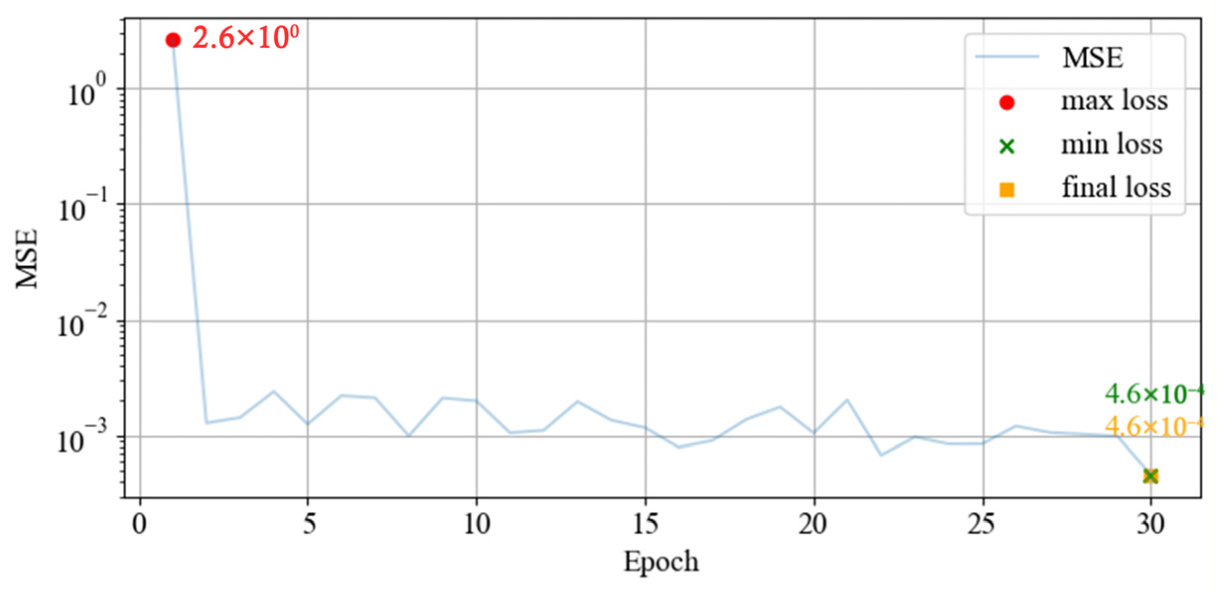
Figure 6 shows the MSE as a function of the number of epochs. In the training process, the maximum number of epochs was set to 100. The parameters used for training are shown in Table 1. The initial MSE was 2.6 and gradually decreased as training progressed, ultimately terminating when it fell below MSEmin. These results indicate that the proposed ANN modeling method converged appropriately and was trained effectively.
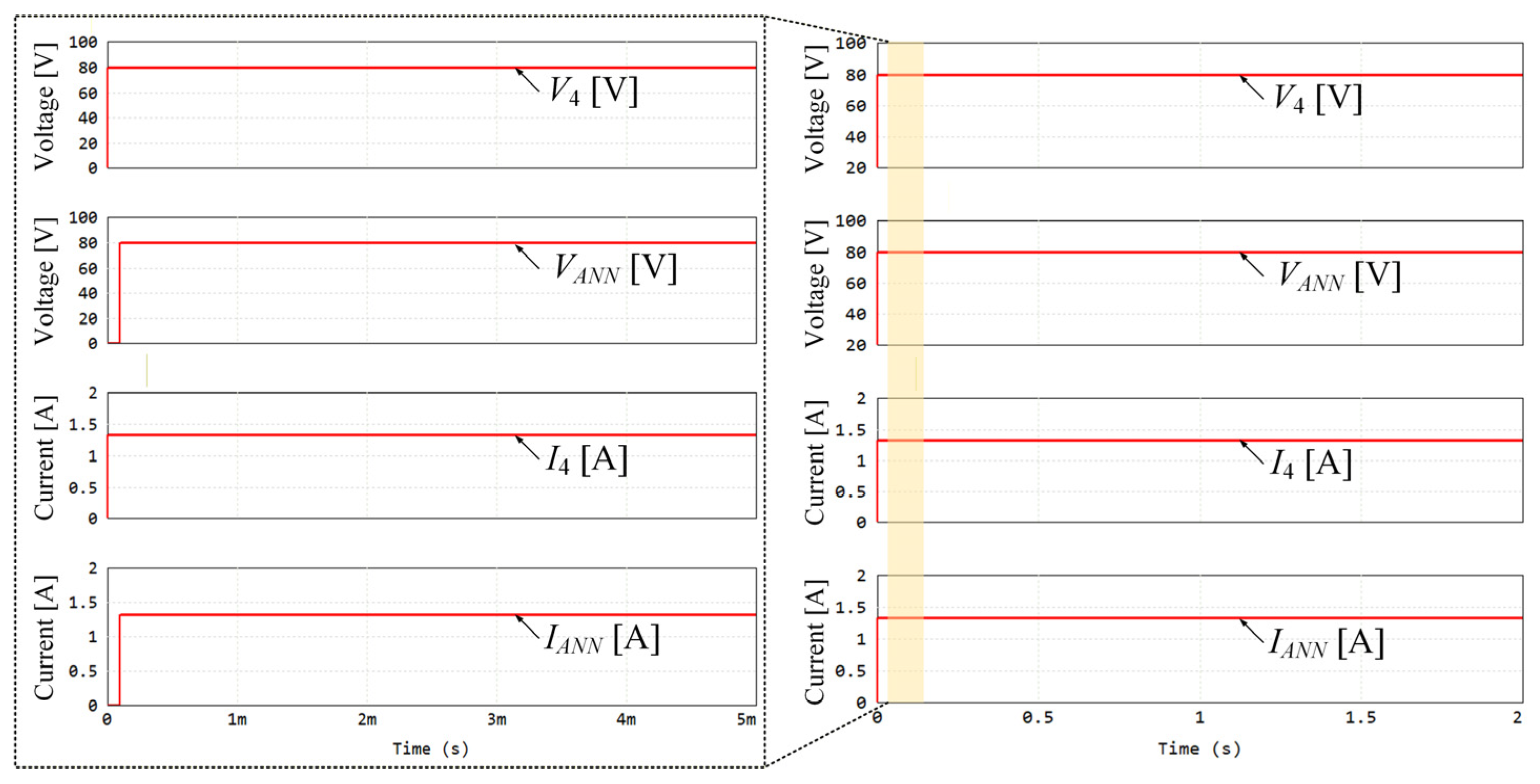
Figure 7 shows the simulation results comparing the voltage and current of resistor 4 and the output of the proposed ANN. The simulation results show that the output voltage (VANN) and output current (IANN) of the ANN accurately predict the V4 and I4. Additionally, the initial operation was verified by enlarging the time interval from 0 to 5 ms, and the ANN outputs were delayed by one sampling due to the initialization of the ANN. After the initial operation, the voltage and current predicted by the ANN closely match V4 and I4, respectively. The proposed ANN modeling method can accurately learn and predict the overall system behavior without the mathematical model of the resistor circuit. By utilizing forward and backpropagation-based modeling, the proposed ANN successfully predicts the voltage and current of resistor 4, thereby verifying the practicality and reliability of the learned model.
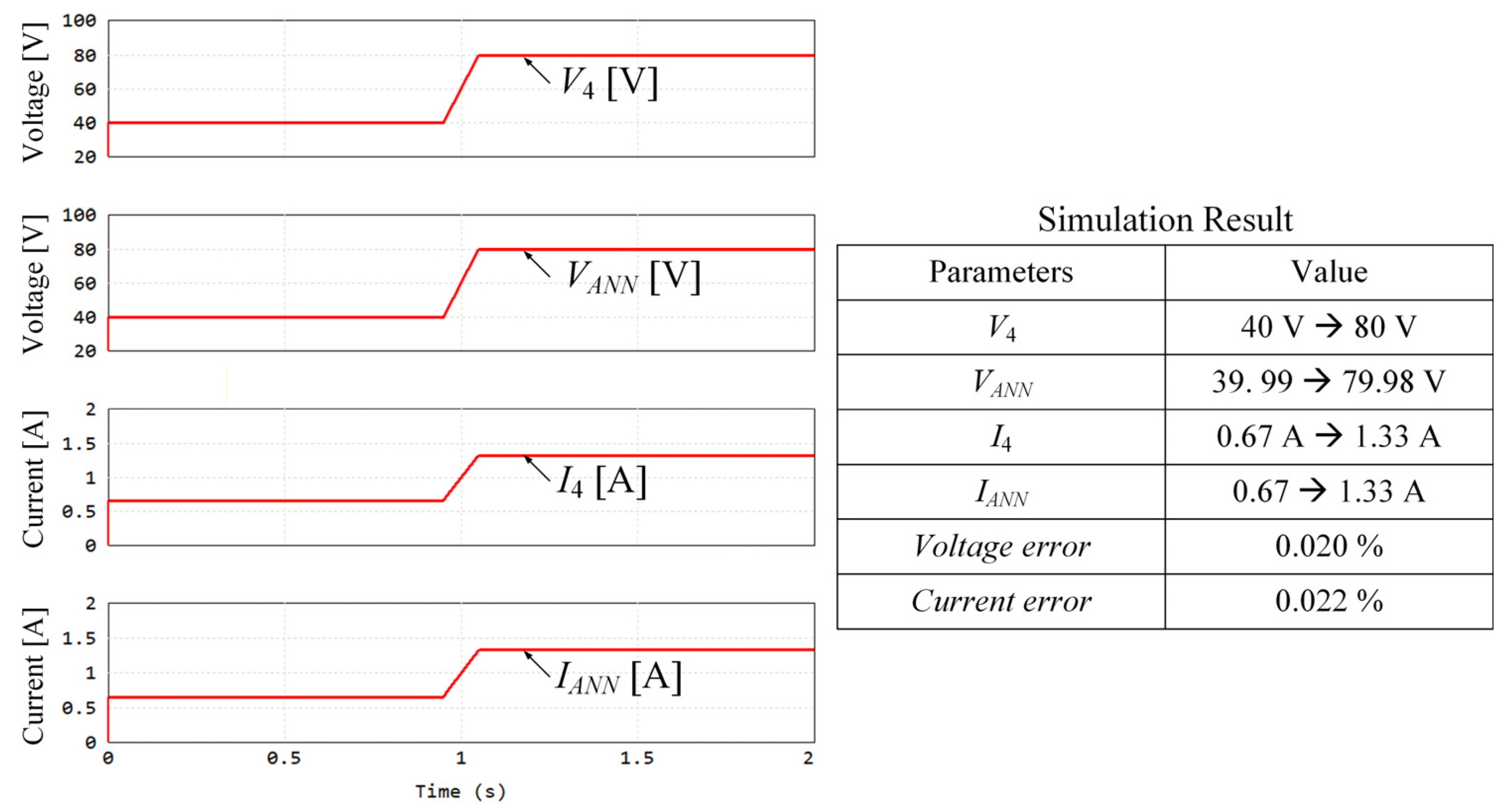
Figure 8 shows the simulation results comparing the voltage and current of resistor 4 and the output of the proposed ANN according to the input voltage. In Figure 7, the input voltage of the resistor circuit is varied from 100 V to 200 V in 0.95 s, and completes the transition over approximately 100 ms. The VANN and IANN accurately predicted the V4 and I4 even in the main parameter variations such as the input voltage that affects the voltage and current of the resistor 4. The proposed ANN maintains high prediction accuracy without retraining, even under varying input voltage, indicating its robustness to parameter variations.
In conclusion, the simulation results predicted by the ANN model method were compared with the simulation results obtained by the conventional mathematical model, and the proposed ANN modeling method has been verified through simulation results to accurately learn and predict the operating characteristics. The error rate of voltage and current predicted through the proposed ANN modeling method was very slight at 0.01975% and 0.0215%. The proposed ANN modeling method can maintain high prediction accuracy without complex mathematical models, and it can be effectively applied to actual systems with parameter variations or nonlinearities.

5. Experimental Results

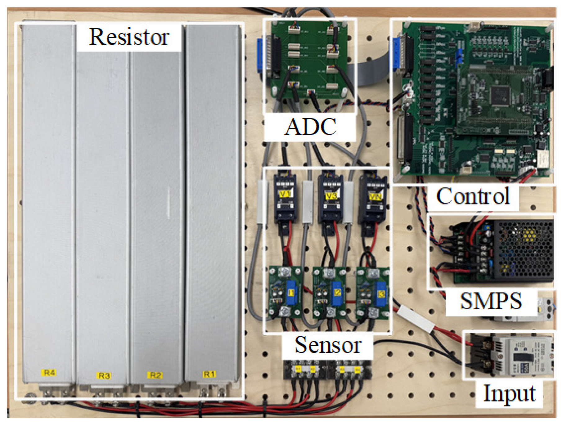
Figure 9 shows the experimental set, which consists of load resistors, an ADC board, a control board, voltage sensors, current sensors, and SMPSs. A DC power supply is used to apply the input voltage to the resistor circuit, and the voltage and current sensors are used to compare the output of the ANN with the actual voltage and current. The effectiveness of the proposed ANN modeling method in this paper is verified through the experimental set. The experimental parameters as shown in Table 1 are used in the simulation, and the parameters used in the experimental set are as shown in Table 2. Voltages and currents are measured through sensors and converted from an analog signal to a digital signal via the ADC board. The converted digital signals are processed by the TMS320F28335 DSP board, which executes the ANN operations. Power for the sensor and the DSP is supplied by SMPSs.
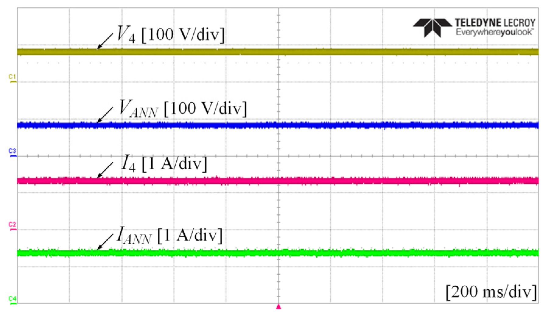
Figure 10 shows the experimental results comparing the voltage and current of resistor 4 and the output of the proposed ANN. The experimental results show that the VANN and IANN accurately predict the V4 and I4. This indicates that the proposed ANN modeling method can accurately learn and predict the system behavior without mathematically modeling the circuit nonlinearities. By utilizing forward and backpropagation-based modeling, the proposed ANN successfully predicts the voltage and current of resistor 4, thereby verifying the practicality and reliability of the learned model.
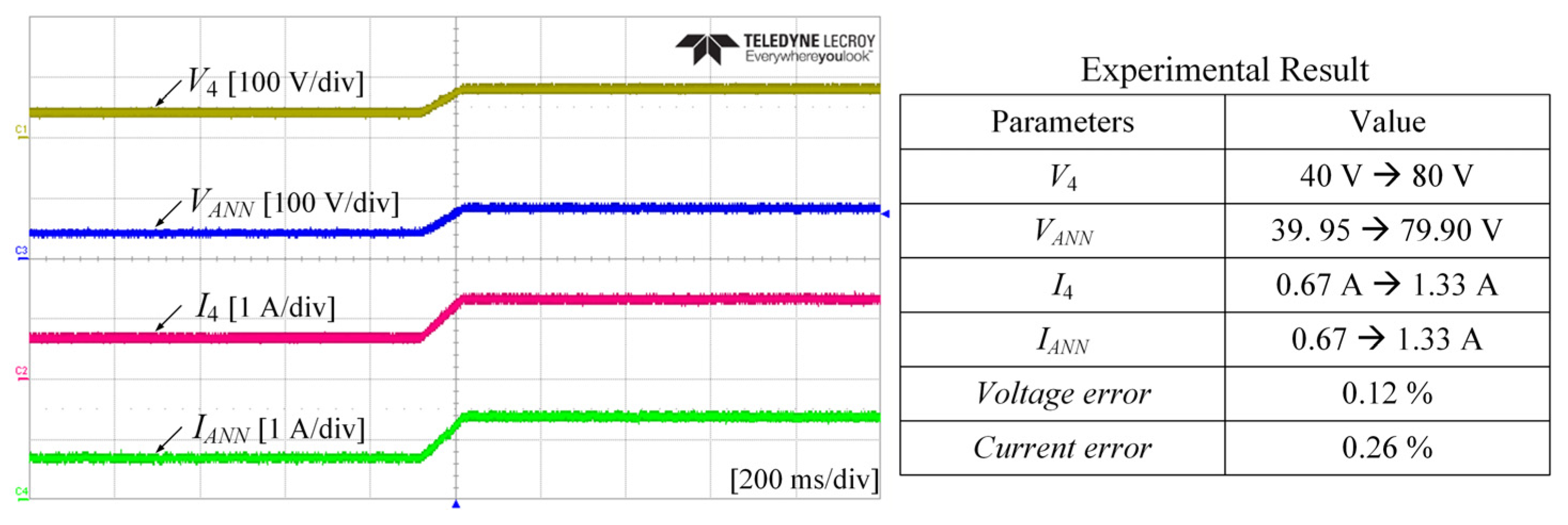
Figure 11 shows the experimental results comparing the voltage and current of resistor 4 and the output of the proposed ANN according to the input voltage. In Figure 10, the input voltage of the resistor circuit is varied from 100 V to 200 V in 0.95 s and completes the transition over approximately 100 ms. The VANN and IANN accurately predicted the V4 and I4 even in the parameter variations such as the input voltage that affects the voltage and current of the resistor 4. The proposed ANN maintains high prediction accuracy without retraining, even under varying input voltage, indicating its robustness to parameter variations.
The experimental results predicted by the ANN model method were compared with the experimental results obtained by the conventional mathematical model, and the proposed ANN modeling method has been verified by experimental results to accurately learn and predict the operating characteristics. The error rate of voltage and current predicted through the proposed ANN modeling method was slight at 0.12% and 0.26%. The proposed ANN modeling method can maintain high prediction accuracy without complex mathematical models. Additionally, it can be effectively applied to actual systems with parameter variations or nonlinearities, and it can be utilized in various power electronics systems.

6. Discussions

This paper focuses on forward and backpropagation-based ANN modeling methods, and the proposed ANN modeling method was verified using an easily interpretable series-parallel resistor circuit. To verify the proposed ANN modeling method, the forward and backpropagation processes were derived step by step and implemented in code. The target variables for verification were set to V4 and I4, which were predicted using the proposed ANN modeling method, and verification was performed by applying dynamic conditions such as input voltage variation. This confirmed its feasibility and predictive performance. This modeling methodology verification is considered a necessary preliminary step before conducting experiments such as sensor noise and temperature experiments, expansion of predicted variables experiments, and applications to PCS experiments.
The proposed ANN modeling method can be extended to PCSs such as DC-DC converters and inverters. Input and output voltage and current, duty ratio, and switching state can be used as input variables. Inductor voltage and current and capacitor voltage and current can be used as output variables. The proposed method can replace sensors and has great potential for application in various fields such as fault diagnosis, operating condition monitoring, and controller design. However, the performance of the proposed ANN modeling method can vary depending on the training parameters. In addition, since it has been verified only on a resistor circuit, its generalizability to other circuits or control algorithms is limited. In future work, the set of predicted variables will be expanded, and the proposed ANN modeling method will be applied to control methods and PCSs. The goal is to simultaneously improve control performance and robustness to parameter variations and disturbances. In addition, the selection of required input variables for PCSs will be conducted while jointly considering performance and cost factors.

7. Conclusions

This paper proposes a forward and backpropagation-based ANN modeling method for PCS. PCS uses sensors to measure voltage and current. However, these sensors require careful tuning across their entire operating range, and are expensive to install and maintain. In addition, these systems are highly sensitive to variations in load conditions, parameter variations, and external disturbances. To address the challenges, the proposed ANN modeling method uses the forward propagation to establish an input–output relationship through weights and biases and the backpropagation to update the weights and biases by minimizing the error between the outputs and the target values. This training process can accurately predict system variables without sensors or mathematical modeling and maintain high prediction accuracy even under varying load conditions and parameter variations. The MSE of the proposed ANN modeling method is about 0.00046, and the prediction errors of the voltage and current verified through simulation and experiment are very small at about 0.01975%, 0.0215%, 0.12%, and 0.26%, respectively. Furthermore, by eliminating the need for sensors, the system structure can be simplified, and the overall cost significantly reduced. The validity of the proposed ANN modeling method was verified by simulation and experimental results.

Author Contributions

Conceptualization, software, simulation validation, writing—original draft preparation, and visualization, G.K.; experimental validation, Y.B. All authors have read and agreed to the published version of the manuscript.

Funding

This research was supported by the National Research Foundation of Korea (NRF) grant funded by the Korea government (MSIT) (No. RS-2025-23323395).

Data Availability Statement

The original contributions presented in this study are included in the article. Further inquiries can be directed to the corresponding author.

Conflicts of Interest

The authors declare no conflicts of interest.

References

  1. Bhardwaj, A.; Moon, J.; Nguyen, D.N.; Pamidi, S.V. A Novel Power Conversion System for SMES in Pulsed Power Applications. IEEE Trans. Appl. Supercond. 2025, 35, 1–5. [Google Scholar] [CrossRef]
  2. Yaramasu, V.; Wu, B.; Sen, P.C.; Kouro, S.; Narimani, M. High-Power Wind Energy Conversion Systems: State-of-the-Art and Emerging Technologies. Proc. IEEE 2015, 103, 740–788. [Google Scholar] [CrossRef]
  3. Park, T.; Kim, T. Novel Energy Conversion System Based on a Multimode Single-Leg Power Converter. IEEE Trans. Power Electron. 2013, 28, 213–220. [Google Scholar] [CrossRef]
  4. Wang, F.; Zhang, Z.; Ericsen, T.; Raju, R.; Burgos, R.; Boroyevich, D. Advances in Power Conversion and Drives for Shipboard Systems. Proc. IEEE 2015, 103, 2285–2311. [Google Scholar] [CrossRef]
  5. Yang, Y.; Mok, K.T.; Tan, S.C.; Hui, S.Y. Nonlinear Dynamic Power Tracking of Low-Power Wind Energy Conversion System. IEEE Trans. Power Electron. 2015, 30, 5223–5236. [Google Scholar] [CrossRef]
  6. Wu, H.; Zhu, L.; Yang, F.; Mu, T.; Ge, H. Dual-DC-Port Asymmetrical Multilevel Inverters with Reduced Conversion Stages and Enhanced Conversion Efficiency. IEEE Trans. Ind. Electron. 2017, 64, 2081–2091. [Google Scholar] [CrossRef]
  7. Habib, S.; Khan, M.M.; Abbas, F.; Ali, A.; Faiz, M.T.; Ehsan, F.; Tang, H. Contemporary Trends in Power Electronics Converters for Charging Solutions of Electric Vehicles. CSEE J. Power Energy Syst. 2020, 6, 911–929. [Google Scholar] [CrossRef]
  8. Kim, M.W.; Kim, H.; Song, M.; Kim, J.J. Energy-Efficient Power Management Interface with Adaptive HV Multimode Stimulation for Power-Sensor Integrated Patch-Type Systems. IEEE Trans. Biomed. Circuits Syst. 2023, 17, 1355–1370. [Google Scholar] [CrossRef]
  9. Guan, M.; Gong, Y.; Mao, R.; Liu, Z.; Tian, B.; Hu, Z.; Liu, M. An External Interference-Resistant Noncontact Voltage Sensor with Negative Feedback Design. IEEE Sens. J. 2024, 24, 17040–17044. [Google Scholar] [CrossRef]
  10. Nibir, S.J.; Biglarbegian, M.; Parkhideh, B. A Non-Invasive DC-10-MHz Wideband Current Sensor for Ultra-Fast Current Sensing in High-Frequency Power Electronic Converters. IEEE Trans. Power Electron. 2019, 34, 9095–9104. [Google Scholar] [CrossRef]
  11. George, O.; Dabas, S.; Sikder, A.; Smith, R.; Madiraju, P.; Yahyasoltani, N.; Ahamed, S.I. State-of-the-Art Versus Deep Learning: A Comparative Study of Motor Imagery Decoding Techniques. IEEE Access 2022, 10, 45605–45619. [Google Scholar]
  12. Kolman, E.; Margaliot, M. Are Artificial Neural Networks White Boxes? IEEE Trans. Neural Netw. 2005, 16, 844–852. [Google Scholar] [CrossRef] [PubMed]
  13. Lang, W.; Hu, Y.; Gong, C.; Zhang, X.; Xu, H.; Deng, J. Artificial Intelligence-Based Technique for Fault Detection and Diagnosis of EV Motors: A Review. IEEE Trans. Transp. Electrif. 2022, 8, 384–406. [Google Scholar] [CrossRef]
  14. Chen, Q.; Dai, X.; Song, X.; Liu, G. ITSC Fault Diagnosis for Five Phase Permanent Magnet Motors by Attention Mechanisms and Multiscale Convolutional Residual Network. IEEE Trans. Ind. Electron. 2024, 71, 9737–9746. [Google Scholar] [CrossRef]
  15. Liu, F.; Wang, X.; Wei, H. Electromagnetic Performance Analysis, Prediction, and Multiobjective Optimization for U-Type IPMSM. IEEE Trans. Ind. Electron. 2024, 71, 10322–10334. [Google Scholar] [CrossRef]
  16. Kang, J.-K.; Yoo, D.-W.; Hur, J. Application and Verification of Voltage Angle-Based Fault Diagnosis Method in Six-Phase IPMSM. IEEE Trans. Ind. Appl. 2024, 60, 426–438. [Google Scholar] [CrossRef]
  17. Tanaka, T.; Kawakami, W.; Kuwabara, S.; Kobayashi, S.; Hirano, A. Intelligent Monitoring of Optical Fiber Bend Using Artificial Neural Networks Trained with Constellation Data. IEEE Netw. Lett. 2019, 1, 60–62. [Google Scholar]
  18. Wu, Z.F.; Li, J.; Cai, M.Y.; Lin, Y.; Zhang, W.J. On Membership of Black-Box or White-Box of Artificial Neural Network Models. In Proceedings of the 2016 IEEE 11th Conference on Industrial Electronics and Applications (ICIEA), Hefei, China, 5–7 June 2016; pp. 1400–1404. [Google Scholar]
  19. Demidova, G.; Justo, J.J.; Lukichev, D.; Poliakov, N.; Anuchin, A. Neural Network Models for Predicting Magnetization Surface Switched Reluctance Motor: Classical, Radial Basis Function, and Physics-Informed Techniques. IEEE Access 2025, 13, 54987–54996. [Google Scholar] [CrossRef]
  20. Fang, Z. A High-Efficient Hybrid Physics-Informed Neural Networks Based on Convolutional Neural Network. IEEE Trans. Neural Netw. Learn. Syst. 2021, 33, 5514–5526. [Google Scholar] [CrossRef]
  21. Park, S.; Suh, T. Speculative Backpropagation for CNN Parallel Training. IEEE Access 2020, 8, 215365–215374. [Google Scholar] [CrossRef]
  22. Wu, S.; Ma, G.; Yao, C.; Sun, Z.; Xu, S. Current Sensor Fault Detection and Identification for PMSM Drives Using Multichannel Global Maximum Pooling CNN. IEEE Trans. Power Electron. 2024, 39, 10311–10325. [Google Scholar] [CrossRef]
  23. Cui, B.; Zhang, S.; Su, J.; Cui, H. Fault Diagnosis for Inverter-Fed Motor Drives Using One Dimensional Complex-Valued Convolutional Neural Network. IEEE Access 2024, 12, 117678–117690. [Google Scholar] [CrossRef]
  24. Rumelhart, D.; Hinton, G.; Williams, R. Learning representations by back-propagating errors. Nature 1986, 323, 533–536. [Google Scholar] [CrossRef]
  25. de Villiers, J.; Barnard, E. Backpropagation neural nets with one and two hidden layers. IEEE Trans. Neural Netw. 1993, 4, 136–141. [Google Scholar] [CrossRef]
  26. Yu, X.; Efe, M.O.; Kaynak, O. A general backpropagation algorithm for feedforward neural networks learning. IEEE Trans. Neural Netw. 2002, 13, 251–259. [Google Scholar]
  27. Deng, J.; Wang, W.; Ning, Z.; Venugopal, P.; Popovic, J.; Rietveld, G. High-Frequency Core Loss Modeling Based on Knowledge-Aware Artificial Neural Network. IEEE Trans. Power Electron. 2024, 39, 1968–1973. [Google Scholar] [CrossRef]
  28. Inoue, K.; Ichige, K.; Nagao, T.; Hayashi, T. Learning-Based Prediction Method for Radio Wave Propagation Using Images of Building Maps. IEEE Antennas Wirel. Propag. Lett. 2022, 21, 124–128. [Google Scholar] [CrossRef]
  29. Yin, Z.; Chen, X.; Shen, Y.; Su, X.; Xiao, D.; Abel, D.; Zhao, H. Plant-Physics-Guided Neural Network Control for Permanent Magnet Synchronous Motors. IEEE J. Sel. Top. Signal Process. 2025, 19, 74–87. [Google Scholar] [CrossRef]
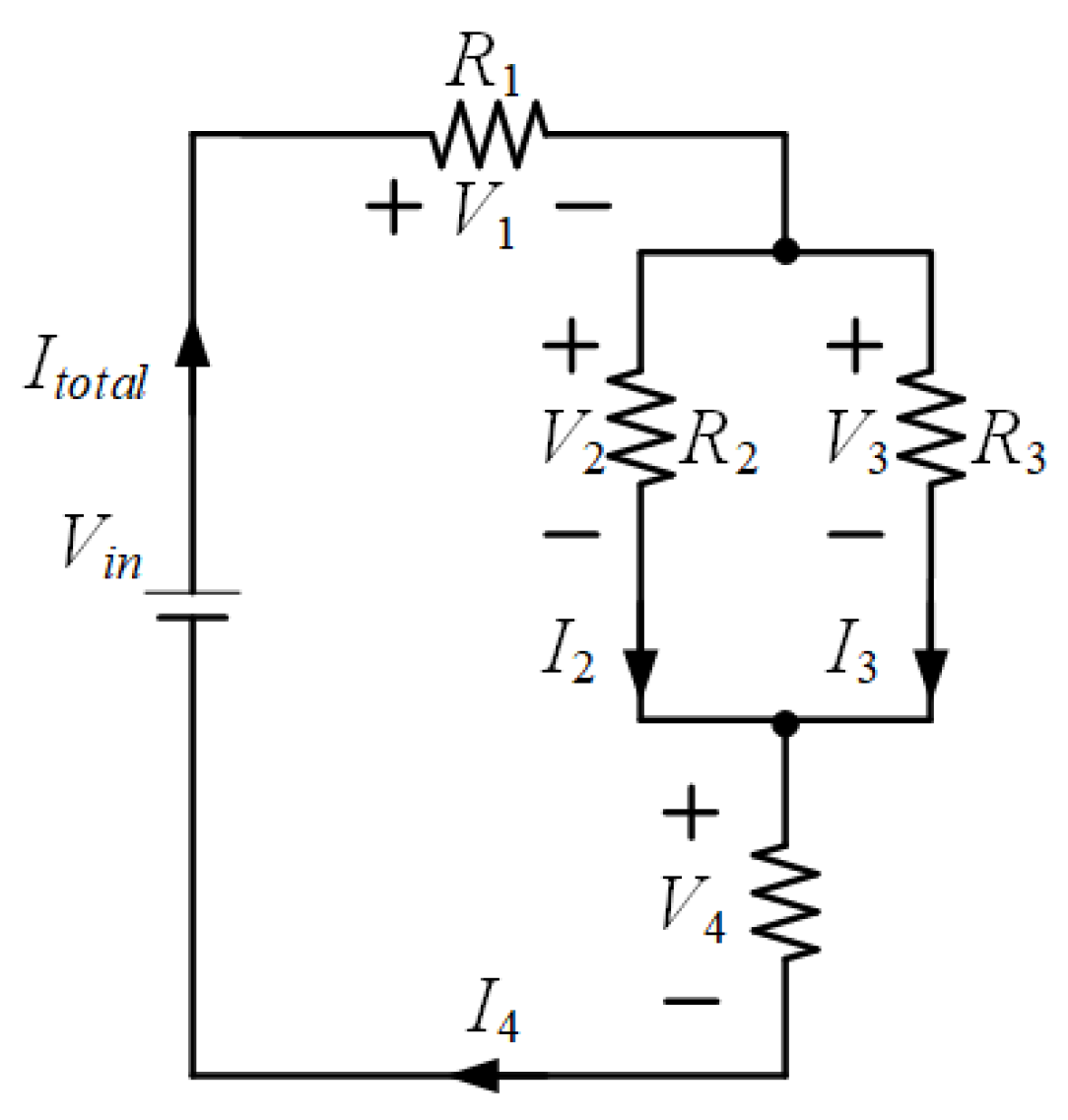
Figure 1. The series-parallel resistor circuit.
Electronics 14 04718 g001
Figure 2. Structure of proposed ANN.
Electronics 14 04718 g002
Figure 3. The forward propagation of the ANN.
Electronics 14 04718 g003
Figure 4. The backpropagation of the ANN.
Electronics 14 04718 g004
Figure 5. The overall training process of the proposed ANN.
Electronics 14 04718 g005
Figure 6. The MSE as a function of the number of epochs.
Electronics 14 04718 g006
Figure 7. The simulation results compared with the voltage and current of resistor 4 and the output of the proposed ANN.
Electronics 14 04718 g007
Figure 8. The simulation results compared with the voltage and current of resistor 4 and the output of the proposed ANN according to the input voltage.
Electronics 14 04718 g008
Figure 9. The experimental set.
Electronics 14 04718 g009
Figure 10. The experimental results compared with the voltage and current of resistor 4 and the output of the proposed ANN.
Electronics 14 04718 g010
Figure 11. The experimental results compared with the voltage and current of resistor 4 and the output of the proposed ANN according to the input voltage.
Electronics 14 04718 g011
Table 1. The series-parallel resistor circuit and ANN parameters.
ParametersSymbolValue
Input voltageVin200 V
ResistorsR1, R2, R3, R460 Ω
The number of neurons in the input layer-1i5
The number of neurons in the first hidden layer-1j9
The number of neurons in the second hidden layer-1k9
The number of neurons in the output layer-1l1
Learning rateη0.001
The number of training iterationsEpoch100
early training stopping criterionMSE < MSEmin5 μ
Table 2. The experimental set parameters.
ParametersValue/ModelPosition
DSP boardTMS320F28335Control
Input voltage200 VInput
SMPSCS30-5, CS30-1212SMPS
Load resistor60 ΩResistor
Voltage sensor800 VmaxSensor
Current sensor25 AmaxSensor
Sampling rate100 μsControl
Disclaimer/Publisher’s Note: The statements, opinions and data contained in all publications are solely those of the individual author(s) and contributor(s) and not of MDPI and/or the editor(s). MDPI and/or the editor(s) disclaim responsibility for any injury to people or property resulting from any ideas, methods, instructions or products referred to in the content.