Article

Apple Scab Classification Using 2D Shearlet Transform with Integrated Red Deer Optimization Technique in Convolutional Neural Network Models

Department of Electrical Electronics Engineering, Zonguldak Bülent Ecevit University, Zonguldak 67100, Türkiye
Electronics 2025, 14(23), 4678; https://doi.org/10.3390/electronics14234678
Submission received: 31 October 2025 / Revised: 24 November 2025 / Accepted: 25 November 2025 / Published: 27 November 2025
(This article belongs to the Section Computer Science & Engineering)

Abstract

Apple is an important fruit worldwide, but it is quite susceptible to various diseases. In particular, apple scab disease (Venturia Inaequalis) is a common fungal infection that causes serious yield losses in apple production. This disease causes spots on both leaves and fruits, negatively affecting product quality and marketability. Early diagnosis and management of apple diseases are critical to increase productivity in apple production. Traditional methods are usually time-consuming and costly; therefore, image processing and artificial intelligence technologies have become important tools in disease detection. In this study, a new approach is developed for the classification of healthy and scab apples by combining image processing, deep learning and optimization methods. First, the dataset is enriched using data augmentation techniques such as rotation, mirroring, zooming, shifting, brightness adjustment, and noise addition. Then, the images are analyzed with Shearlet Transform (ST), and frequency and spatial features are extracted in detail. The features obtained from the ST are reconstructed with the inverse transformation, and the original images are given as inputs to deep learning architectures, specifically AlexNet, VGG-16 and ResNet-18. In each model, deep features are extracted to classify healthy and scab apple images, and a feature pool is created by combining these features. The selection process of features that will increase performance in the classification process is carried out with the Red Deer Optimization (RDO) algorithm. This algorithm, inspired by the natural life cycle of male deer, includes the steps of determining the leader deer, creating a harem, mating and selecting the next generations. By selecting the best male leaders and optimizing the mating process, the algorithm ensures that the most effective feature combinations are chosen to enhance classification performance. As a result, this hybrid method presents an innovative approach to accurately classifying healthy and scab apple images, contributing to more efficient and reliable disease detection in apple production.

1. Introduction

As the world’s population increases, maximizing yield per unit of cultivated land is of vital importance for both food security and environmental sustainability [1]. Plant agriculture and fruit growing, which include the cultivation of plants such as grains, vegetables, fruits, legumes, oilseeds and flowers, are considered the cornerstones of food production [2,3]. Fruit growing is an agricultural activity that includes the production of quality fruit saplings, the cultivation of fruit trees and plants, and the realization of fruit production [3]. In order to ensure the healthy growth of fruit trees, operations such as planting saplings suitable for the relevant fruit type [3], appropriate irrigation [4], fertilization [5], pruning operations [6], disease and pest control [7] should be carried out. According to FAOSTAT (FAO, 2022) data, apple production worldwide in the last 10 years has ranked third in fruit production with an annual production of 80 million tons [8,9]. Research and development studies for apple cultivation have the potential to increase productivity by reducing the production costs of apples, a commercial fruit product [9]. Additionally, leaf diseases [10] and fruit diseases [11] are among the main factors that directly affect apple production and productivity. When the literature is examined, it is seen that Gymnosporangium juniperi-virginianae, Venturia inaequalis and Botryosphaeria obtusa are fungal pathogens that affect apple trees [12,13,14,15,16]. Gymnosporangium juniperi-virginianae is a fungal pathogen that causes a plant disease known as Cedar-Apple Rust [12]. This plant disease affects apple and cedar trees. It can cause significant damage to apple trees and reduce fruit quality. Control of Cedar-Apple Rust is generally done to minimize the spread of the disease on both host plants [12]. Another fungal pathogen, Botryosphaeria obtusa, is associated with fruit trees, particularly apples, pears and grapevines [13]. Commonly known as the Black Rot fungus, this pathogen can cause serious damage to fruit trees, causing problems such as cankers, dieback and fruit rot. Control and management of Botryosphaeria obtusa generally involves strategies such as pruning out infected branches, applying fungicides and maintaining proper tree hygiene and maintenance to minimize its impact on fruit tree health [14]. Another harmful pathogen is Venturia inaequalis, the scientific name for the fungal pathogen that causes apple scab [15]. Apple scab is a common and devastating disease affecting apple trees and can lead to reduced fruit quality and yield. The fungus infects the leaves, fruit, and shoots of apple trees, causing distinctive scab-like lesions and spots on the surface of the fruit. Control and management of Venturia inaequalis generally involves a variety of strategies, including the use of fungicides, disease-resistant apple tree varieties, and cultural practices such as pruning [16]. Monitoring agricultural products is significantly enhanced by apple scab detection. This is a critical step in maintaining product quality and preventing yield losses. The most common method for monitoring the condition of agricultural products is visual inspection; however, the obvious disadvantage of this method is the inability to detect diseases in the early stages of development due to the lack of visible symptoms. Furthermore, due to the large volume of orchards, not every plant can be examined, leading to selective monitoring, which significantly reduces the quality of monitoring [17].

1.1. Current Approaches in the Literature

In a previous study, data collection and then training of a deep learning model are carried out to detect apple diseases [18]. Two different datasets are created, one with scab and healthy fruits and one with scab and healthy fruit tree leaves. The effect of transfer learning in dataset selection for apple diseases is examined by comparing the transfer learning approach with the scratch learning approach. Statistical analysis is shown to confirm the positive effect of transfer learning on Convolutional Neural Network (CNN) performance with a significance level of 0.05 [18]. In another study, a dataset is collected for the detection of early apple disease and a CNN model based on the sliding window method is developed [19]. The CNN model is trained using the transfer learning approach on the MobileNetV2 architecture tuned for embedded devices. In the recognition study conducted in a laboratory environment, the F1-score value of the model created on the collected data is obtained as 96% [19]. In another study, a CNN model that requires less storage space and shorter processor speed is created and a disease detection study is conducted on apple tree leaves [20]. A dataset is created using data diversity methods to classify the Scab, Black rot, and Cedar Rust diseases. It is stated that the trained CNN model has a classification performance of 98% and that the created model can be integrated into portable devices [20]. In [21], an automatic system including multispectral scanners and various sensors is proposed for the inspection of apple orchards and early disease detection. The system consists of a mobile platform and a camera-based detection system. The F1-score value of the model based on artificial neural networks is obtained as 98.3%, 97% and 97.2% for the healthy, rot and cedar rust classes, respectively [21].
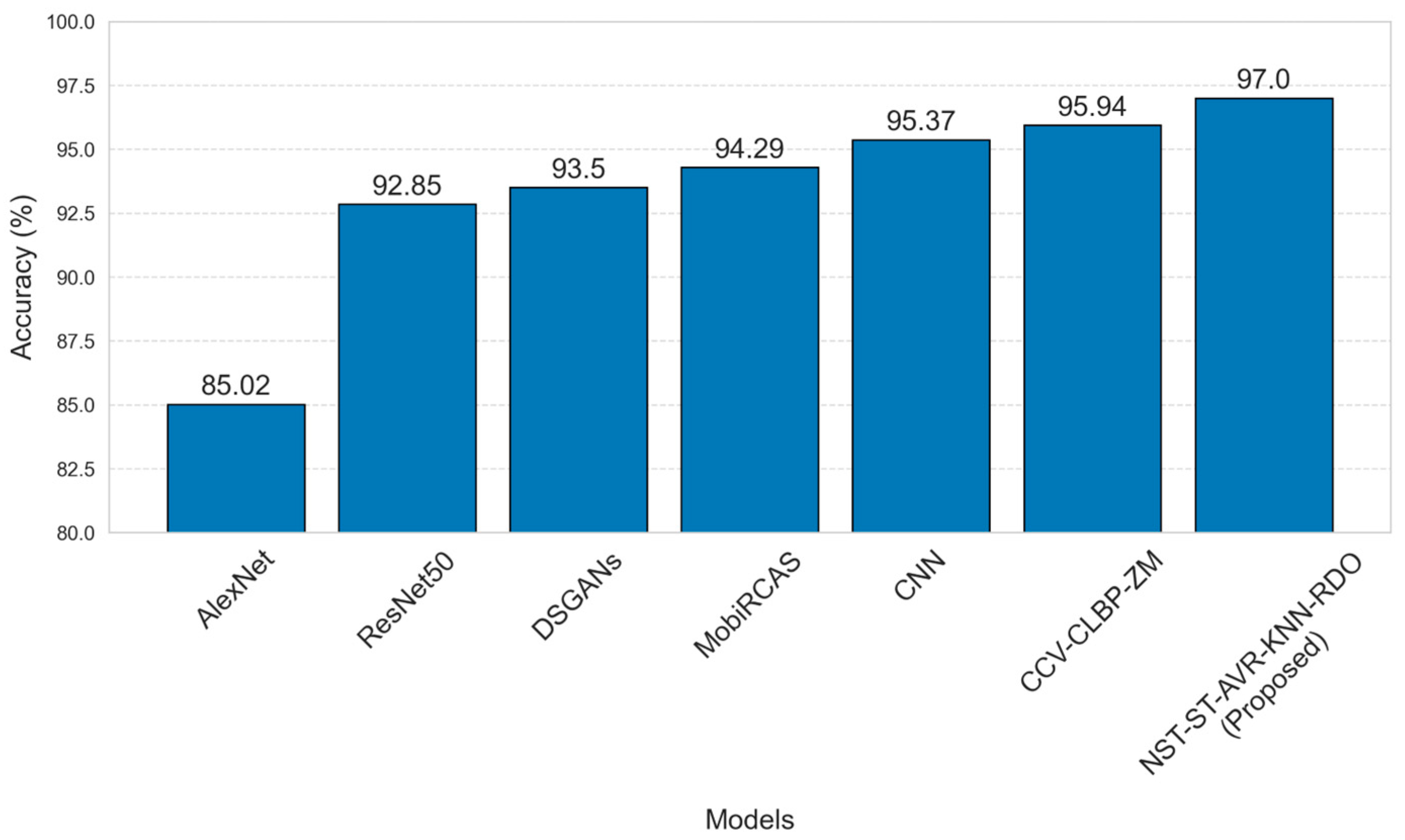
In a previously conducted study, image processing is used to classify apple diseases, where diseased regions in apples are detected using the K-means clustering method [22]. Subsequently, color, texture, and shape features are calculated and combined to create a single descriptor. Finally, a multi-class support vector machine is employed to classify the apples as either healthy or diseased. With the model named CCV + CLBP + ZM, they achieve a success rate of 95.94% [22]. In [23], a real-time method is proposed for the simultaneous classification and segmentation of apple diseases. Based on a UNet and ResNet system, the model they named MobiRCAS achieves a classification performance of 94.29%. In [24], a new method is proposed for the classification of diseased and healthy apples using a deep learning technique. Images of normal apples along with images related to three apple diseases (Blotch, Rot, and Scab) are used in the model. The data is augmented, and ResNet-50, a convolutional neural network, is employed as the prediction model for multi-class classification. Subsequently, the performance is measured through accuracy, achieving a success rate of 80.95% for scab, with an overall success rate of 92.85%. In [25], an innovative CNN model is proposed to detect and classify apple diseases (Scab, Rot, Blotch). With reduced layers to ease computational load, the model achieves 95.37% accuracy overall, with an 80% detection rate for Scab, while being fast and efficient. In the study [26], the Deep Spectral Generative Adversarial Networks (DSGANs) algorithm is proposed to detect apple diseases. Images are preprocessed using Median and Gabor Filters, and boundaries are determined with the Canny edge detector. The SAPHE technique separates affected and healthy regions, while ISWS optimizes segmentation. Features are extracted using ReLu activation and GAN layers for disease classification. The proposed method achieves an average performance of 93.50%.

1.2. Motivation and Contributions

This study investigates the impact of data augmentation techniques on enhancing the performance of deep learning models with limited real datasets, particularly to achieve more reliable results in the classification of agricultural products (e.g., healthy and scab-affected apples). In the literature, there is insufficient research on the applicability of data augmentation techniques to agricultural datasets, and the effect of Shearlet Transform (ST) on CNN models remains underexplored. Additionally, there are gaps in the comparative analysis of emerging optimization techniques, such as the Red Deer optimization method, against genetic algorithms (GA), as well as in the hybrid evaluation of machine learning and deep learning approaches. This study aims to address these shortcomings and provide a practical solution. This work generates a balanced dataset of 3000 samples by producing 2372 augmented data points from 628 real data points, and subsequently splits the data into 80% training and 20% testing sets to systematically evaluate model performance. The effect of ST on CNN-based models (AlexNet, VGG-16, ResNet-18) is analyzed in detail. The study also conducts a comparative evaluation of the Red Deer optimization method against GA and incorporates machine learning methods such as KNN, and thereby provides a multifaceted contribution to the literature. These findings demonstrate the practical applicability of data augmentation and signal transformation techniques in agricultural data analysis, and addresses gaps in areas such as plant disease detection and classification.

2. Methodology

This section explains in detail the components of the proposed novel apple scab classification model. In the first stage, detailed information about the proposed framework is given. In the following sections, the parts of the apples in the dataset are labeled, and a new dataset is obtained for both healthy and scab apples. Data augmentation techniques such as rotation, mirroring, zooming, shifting, brightness adjustment, and noise addition are explained. Detailed mathematical background regarding 2D-ST is given. Information is given about AlexNet, VGG-16 and ResNet-18, which are deep learning approaches used to extract relevant features. The methods used in this study are explained in detail in the following sections.

2.1. Proposed Framework for Apple Scab Classification Model

In this study, a novel model for apple scab classification is proposed, based on 2D-ST, the Deep Learning approach and the Red Deer Optimization (RDO) approach. After the labeling process is performed on the collected raw data, a data augmentation process is performed and then 2D-ST is applied to obtain two different data sets. Both the original data set and the images obtained as a result of the 2D-ST and Inverse 2D-ST are utilized in AlexNet, VGG-16 and ResNet-18 deep learning models. The most relevant features obtained from these models are identified with the RDO approach and the classification process is completed with the KNN approach. The process of detecting apple scab is evaluated for different hybrid approaches by measuring different metrics.
The framework of the proposed approach is provided in Figure 1. If we briefly explain these stages, they can be listed as follows:
1. Preprocessing Stage: In this stage, augmentation techniques are applied to generate the training and test datasets for model training from the original apple images.
2. Signal Processing Stage: In this stage, the Shearlet and inverse Shearlet Transform are applied to the augmented data to generate a separate dataset.
3. Feature Extraction Stage: Features are extracted separately using transfer learning methods for both the data without ST and the data with ST applied.
4. Optimization Stage: The Red Deer Optimization approach is used to investigate the most suitable features.
5. Classification Stage: The performance of the classifiers is compared based on the obtained features, and the model yielding the highest success rate is identified.

2.2. Dataset

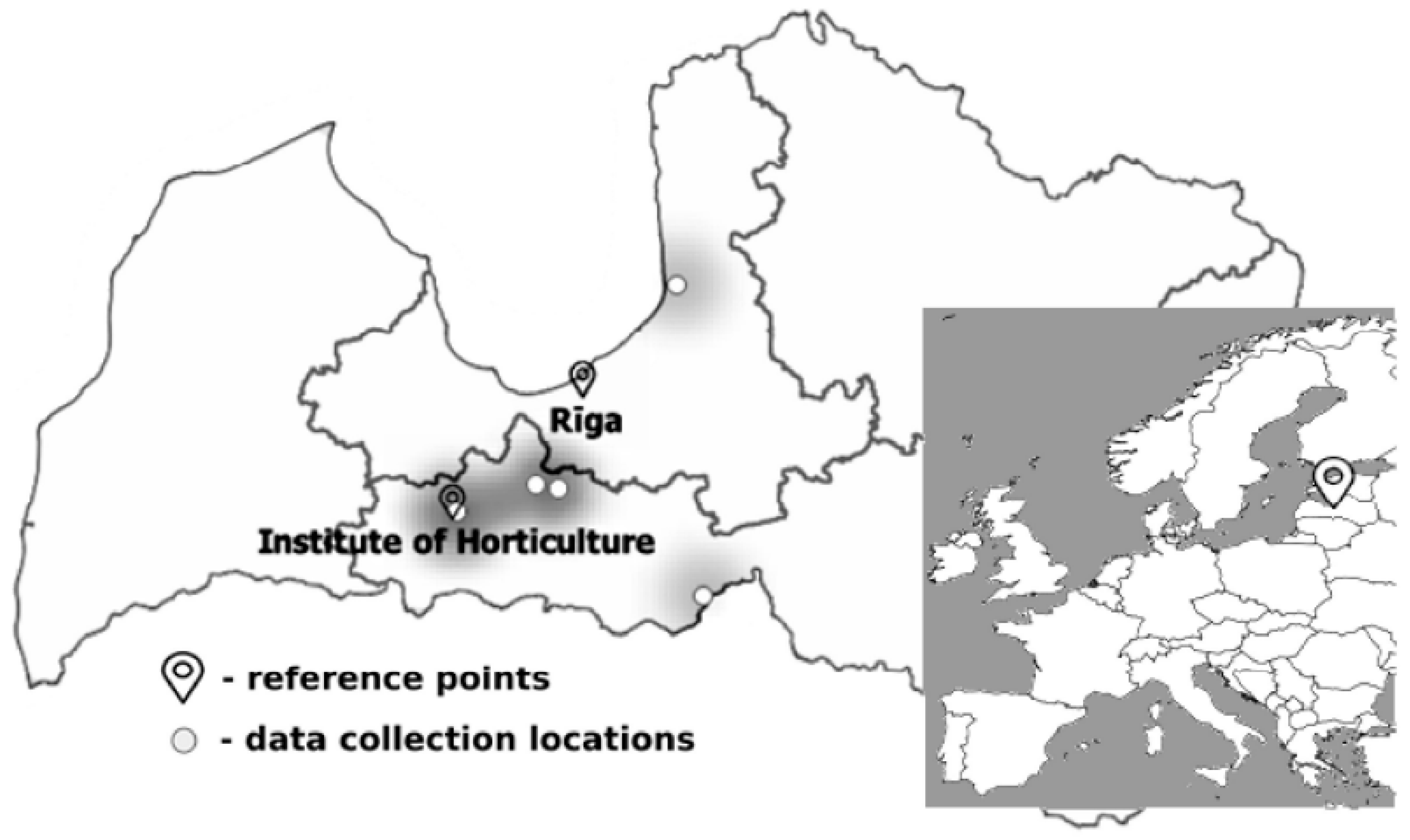
The study uses a dataset consisting of photographs containing 90 healthy and 207 apple scab images [18]. Digital images are collected from apple trees showing signs of rot in different regions of Latvia (Figure 2). Digital images on leaves and fruits showing characteristic signs of rot are collected from six different locations: a horticultural institute (LatHort), a commercial orchard, and a home garden. Data collection is carried out throughout the apple growing season. It continues from the beginning of June 2020, when the first signs of apple scab infection began to appear on the leaves, until the end of September 2020, when both leaves and fruits showed other pest symptoms that prevents differentiation from apple scab at the end of the growing season [18].

2.3. Data Labeling

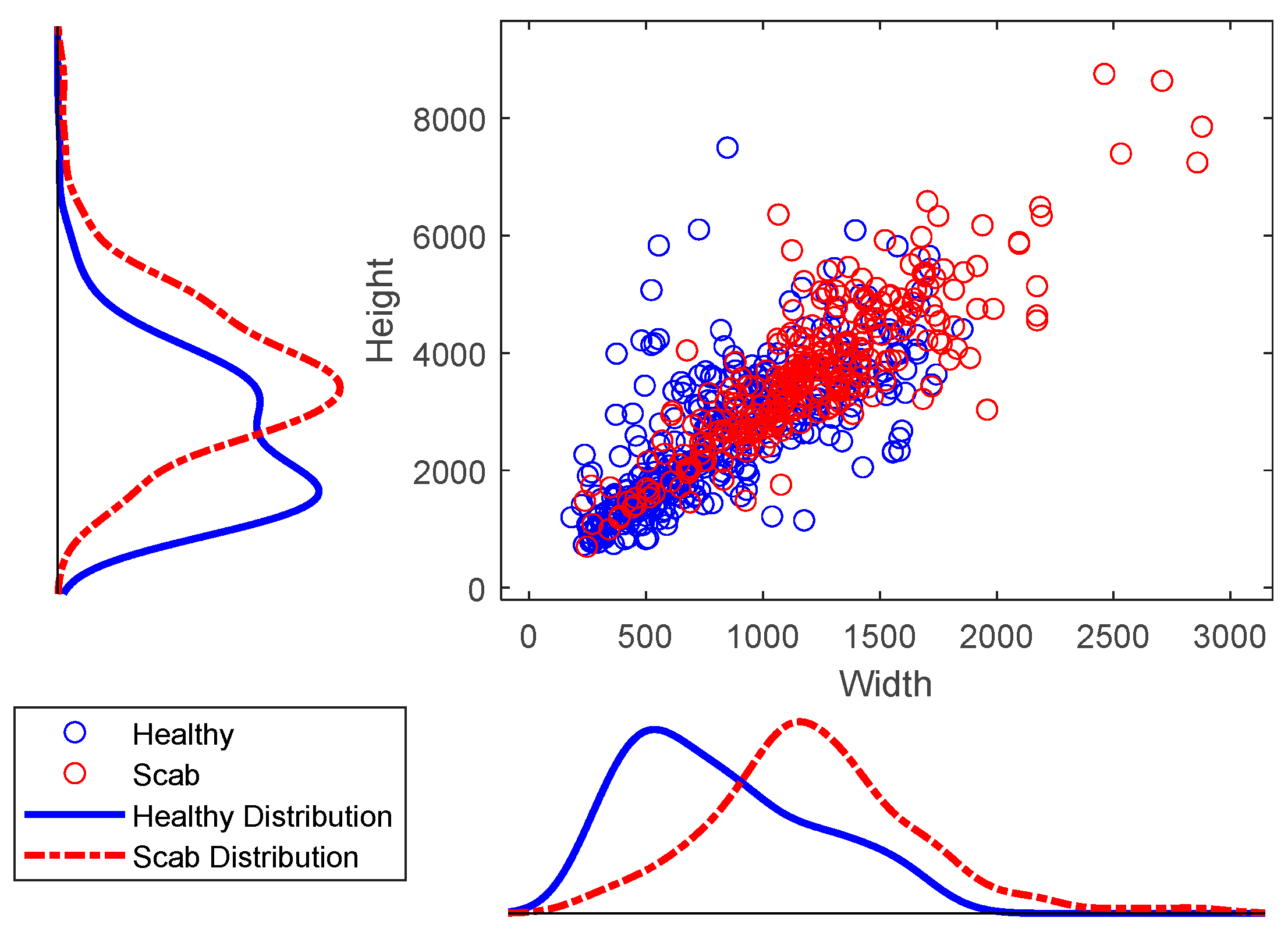
Since the dataset can contain more than one apple in an image, the labeling process is performed. At the end of the labeling process, 345 healthy and 283 scab apple images are obtained. The resolution distributions of the apple images are obtained after the labeling process and are shown in Figure 3 for both healthy apple images and scab apple images. It is seen that the average values of the resolution distributions of the images in both groups are different. However, the size of the scab apple images is larger than the size of the healthy apple images on average. Apart from the fact that the number of scab apple images is low compared to the number of healthy images, the fact that the size is large compared to the healthy apple images shows that relatively more detailed features can be extracted.

2.4. Data Augmentation

Data augmentation is a technique used to artificially expand training data in order to improve the performance of machine learning models. This method is particularly useful for enhancing the generalization capabilities of deep learning models and preventing overfitting [27]. Approaches such as rotation, flipping, and shifting from image-based transformations [28], as well as pixel-based modifications like brightness adjustments [29], and adding noise [30], are commonly used.

2.4.1. Rotation

In data augmentation, images are rotated at specific angles (θ) to enable the model to learn from different perspectives. This process involves the spatial transformation of pixel coordinates and is typically used to change the orientation of an image. It helps the model generalize more effectively with rotated images [31]. Rotation is performed in a 2D plane using a rotation matrix (M) as in Equation (1).
M = cos θ sin θ sin θ cos θ
The new coordinates (x′, y′) are calculated from the old coordinates (x, y) as in Equation (2).
x y = M . x y = xcos θ sin θ x sin θ cos θ
Here, θ represents the counterclockwise rotation angle; for rotation around a center, coordinates are first shifted relative to the center, transformed using the rotation matrix, and then shifted back, with pixel coordinates converted and placed in new positions via interpolation (e.g., bilinear), as used in operations like rotating a photo by 90°.

2.4.2. Flipping

Flipping images horizontally or vertically is one of the data augmentation techniques. This method is especially useful for datasets containing symmetrical objects [32]. Horizontal flipping is expressed by Equation (3), while vertical flipping is expressed by Equation (4).
( x , y ) ( w x 1 , y )
Here, w is the width of the image. This reverses the x-coordinate of each pixel with respect to the width.
( x , y ) ( x , h y 1 )
h is the height of the image. This reverses the y-coordinate with respect to the height.

2.4.3. Zooming

By zooming in on a random region of the image, the model can recognize objects of different sizes. This teaches the model to understand objects from different scales [33]. The image is enlarged by a zoom factor and typically cropped from the center to highlight details. The mathematical basis is as follows: the new dimensions are calculated as in Equation (5).
( n e w w , n e w h ) ( w . z , h . z )
where w is the original width, h is the original height, and z is the zoom factor (e.g., z > 1 for enlargement, z < 1 for reduction). Then, the new image is cropped from the center so that only the magnified area is visible.

2.4.4. Shifting

The positions of objects in the image are shifted horizontally or vertically. This improves the model’s ability to recognize objects in different locations [28]. The image is shifted by a certain amount horizontally (Δx) and vertically (Δy), as expressed in Equation (6). This alters the spatial alignment of the frame.
( x , y ) ( x + x , y + y )

2.4.5. Brightness and Contrast Adjustment

By adjusting the brightness levels of images, the model becomes more robust to changes in lighting conditions. This simulates different lighting environments [34]. Pixel intensities are adjusted using brightness (β) and contrast (α) parameters to simulate lighting conditions. The mathematical basis is as in Equation (7).
I x , y = α . I x , y + β
Here, α represents the contrast factor (α > 1 increases contrast, α < 1 decreases it), while β denotes the brightness shift value (positive values increase brightness, negative values decrease it).

2.4.6. Adding Noise

Random noise is added to the image to make the model more resilient to noisy data. This is especially useful for handling distortions encountered in the real world [35]. Random noise from a Gaussian distribution, representing real-world distortions, is added to the image, with the mathematical basis defined as in Equation (8).
N x , y i . i . d . N ( μ , σ 2 ) , x , y
where μ is the mean and σ 2 is the variance (noise intensity), resulting in the new pixel value I x , y as in Equation (9).
I x , y = I x , y + N ( x , y )

2.4.7. Adding Salt and Pepper Noise

For each pixel with a probability p, pixels are randomly set to 0 (black, ‘pepper’) or 255 (white, ‘salt’), mimicking impulsive noise known as salt-and-pepper noise [36]. The probability density function is defined as in Equation (10).
I x , y = p 2 f o r   I x , y = 0 p 2 f o r   I x , y = 255 1 p f o r   I x , y = I x , y
This function describes the probability of a pixel being set to 0 (black) or 255 (white), each with probability p/2, or remaining its original value I with probability 1 − p, effectively modeling impulsive salt-and-pepper noise.

2.4.8. Cropping

Cropping is a data augmentation technique that reduces the risk of overfitting and enhances the performance of deep learning models, especially on small-scale datasets [37]. The image is scaled down by a specific ratio and cropped from a random starting point ( x 0 , y 0 ) , limiting the field of view, with the new dimensions defined as in Equation (11).
( n e w w , n e w h ) ( w . s , h . s )
where w and h are the original width and height, s is the scaling factor (0 < s < 1); the cropping is performed such that the randomly selected starting point ( x 0 , y 0 ) satisfies 0 ≤ x 0 ≤ w − n e w w and 0 ≤ y 0 ≤ h − n e w h , limiting the field of view [30].
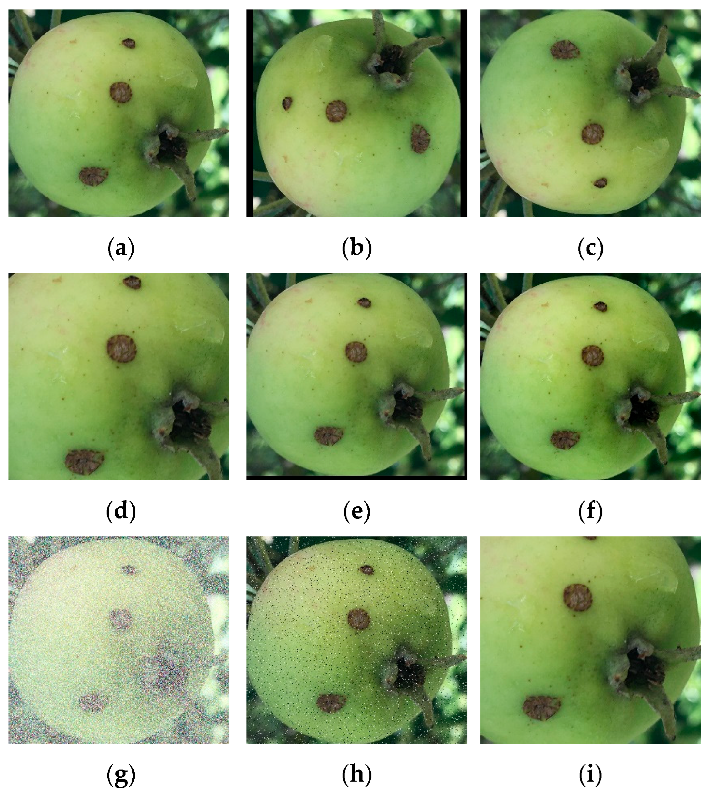
An example of the data augmentation techniques applied in this study, along with the specific parameter values used, is visualized in Figure 4. In this example, the effects of the applied transformations are shown alongside (a) the original image. These effects include, respectively: (b) a 90-degree rotation; (c) a vertical flip; (d) a 1.35× magnification (zoom); and (e) translation (shift) by −14 pixels on the x-axis and −21 pixels on the y-axis. The pixel-based modifications are performed by adjusting (f) the brightness to −17 and the contrast to 1.13. Furthermore, among the noise addition methods, (g) Gaussian noise is applied with a mean of 0 and a standard deviation of 14.23, and (h) Salt and Pepper noise is added with a probability value of 0.03. Finally, (i) a cropping operation is presented, defined by a ratio of 0.76 and starting coordinates of x = 203 and y = 194. This detailed example demonstrates the scope of data variations created to enhance the model’s generalization capability.

2.5. 2D Shearlet Transform

The Shearlet Transform (ST) is a powerful mathematical tool used in multidimensional data processing and analysis. Developed to overcome the limitations of traditional Wavelet Transforms (WT), such as directional deficiencies, the ST demonstrates optimal performance, particularly in representing images containing edges, corners, and other geometric features [38,39]. The ST is a multi-scale and directional transform that captures signal details at different scales and orientations, facilitating signal-noise separation [40]. Thanks to these properties, the ST is effectively used in various applications such as image processing, video enhancement, and microseismic data denoising [40,41].
The mathematical foundation of the ST is based on scaling, translation, and shearing operations. The ST ( ψ ) is generally expressed as in Equation (12).
ψ a , s , t ( x ) = a 3 4 ψ A a 1 S s 1 x t
where the scale parameter a > 0, the shear parameter s ∈ℝ and the translation parameter t ∈ℝ2, which control the scaling, shearing, and positioning of the function, respectively. The anisotropic scaling matrix is defined also as in Equation (13), and the shear matrix is defined as in Equation (14), respectively.
A a = a 0 0 a
S s = 1 s 0 1
This formulation highlights the directional sensitivity and scaling capability of the ST. The continuous ST is defined for a signal f(x) as in Equation (15).
S H ψ f a , s , t = f , ψ a , s , t = R 2 f x ψ a , s , t x ¯ d x
where S H ψ f a , s , t represents the Shearlet coefficients, f , ψ a , s , t denotes the inner product, and ψ a , s , t ( x ) ¯ is the complex conjugate of the Shearlet function. The discrete Shearlet system is defined using the scale j, direction k, and location m parameters as in Equation (16).
ψ j , k , m ( x ) = 2 3 j 2 ψ S k A 2 j x m
This transform exhibits superior performance compared to wavelet-based methods in the processing of multicomponent and multidimensional data, particularly in tasks such as edge and corner detection [38]. The ST is chosen because it is an optimally sparse representation for multidimensional functions characterized by smooth edges, which aligns perfectly with the requirements of the task at hand. This superior representation capability is formalized by the fact that the ST provides the provably sparsest representation for functions with singularities along C 2 (twice differentiable) curves [39].

2.6. Deep Learning Models

Deep learning is a field of artificial intelligence that uses artificial neural networks to extract features from data and make predictions [42]. These models typically operate using multi-layered networks (deep networks) and are effective in areas such as image processing [43], speech recognition [44], and more. CNNs, Recurrent Neural Networks (RNNs), and transformer-based models are commonly used types. Transfer learning enables a pre-trained model to apply the knowledge it has learned to a new problem [45]. This accelerates the training process and allows for high accuracy with smaller datasets. While deep learning requires large datasets and significant computational power, transfer learning reduces these requirements [46].

2.6.1. AlexNet

AlexNet is a pioneering CNN architecture developed by Alex Krizhevsky, Ilya Sutskever, and Geoffrey Hinton in 2012, representing a major breakthrough in deep learning and computer vision [47]. AlexNet captured widespread recognition by securing a decisive victory in the ImageNet Large Scale Visual Recognition Challenge (ILSVRC), demonstrating the immense potential of deep learning in the field of computer vision. AlexNet consists of 8 layers: 5 convolutional layers and 3 fully connected layers. The convolutional layers use filters to extract local features from images, while the fully connected layers are used for classification. AlexNet accelerated the training process and achieved better performance by using the ReLU (Rectified Linear Unit) activation function. It also employed the dropout technique to prevent overfitting [47]. AlexNet enabled training on large-scale datasets by performing parallel computation on GPUs, allowing deep learning models to be trained faster and more efficiently. The success of AlexNet paved the way for the widespread adoption of deep learning in artificial intelligence and machine learning fields. Today, the core principles of AlexNet form the foundation of many modern CNN architectures.

2.6.2. VGG-16

VGG-16 is a significant CNN model developed by the Visual Geometry Group (VGG) at the University of Oxford in 2014 [48]. It stands out for its high performance in image classification and other visual recognition tasks. The model is named after its 16-layer architecture, consisting of 13 convolutional layers and 3 fully connected layers. The most notable feature of VGG-16 is its use of only 3 × 3 convolutional filters. These small filters help the network learn deeper and more complex features in each layer. The layers of the model are typically grouped into several convolutional layers followed by a pooling layer. Pooling reduces the size of the data while preserving important features. VGG-16 has been trained on large datasets such as ImageNet and has achieved highly successful results. As a result, the model is effectively used in various visual recognition tasks through transfer learning methods. Compared to other deep learning models, VGG-16′s architecture is simpler and more regular because all convolutional layers consist of the same 3 × 3 filters. However, this simplicity results in a large number of parameters, which increases the computational cost. Nevertheless, due to its strong generalization capabilities, VGG-16 is widely used in various visual analysis applications [48].

2.6.3. ResNet-18

ResNet-18 (Residual Network) is a CNN architecture developed by Microsoft Research in 2015, representing a significant breakthrough in deep learning [49]. ResNet introduced the concept of Residual Learning to overcome the challenges faced in training very deep networks. ResNet-18 is a smaller and lighter version of this architecture, consisting of 18 layers. The key innovation of ResNet is the use of residual connections. These connections add the input of a layer directly to its output, making it easier for the network to learn. This helps to reduce the vanishing gradient problem that is commonly seen in traditional deep networks and enables the successful training of much deeper networks. ResNet-18 contains 16 convolutional layers and 2 fully connected layers, utilizing these residual blocks. ResNet-18 demonstrates high performance in computer vision tasks such as classification, object detection, and segmentation. It has been trained on large datasets like ImageNet, achieving impressive results in terms of both accuracy and computational efficiency. Compared to larger ResNet models (such as ResNet-50, ResNet-101), ResNet-18 has fewer parameters, making it suitable for use in resource-constrained environments. ResNet-18 has become a reference point in the design of deep learning models, and residual connections are now a standard feature in many modern architectures. This has made the training of deeper and more powerful models possible [49].

2.7. Red Deer Optimization Method

The Red Deer Optimization Method (RDA) is a novel nature-inspired meta-heuristic algorithm developed based on the behaviors of Scottish red deer during the breeding season. This algorithm falls within the category of population-based meta-heuristic methods and uses red deer (RDs) as its initial population. This population is divided into two groups: female deer (hinds) and male deer. A harem is a group of female deer gathered together, and male deer compete to obtain a harem with more female deer. This competition is carried out through the roaring and fighting behaviors of male deer [50,51]. RDA has demonstrated superiority in solving various engineering and multi-objective optimization problems. The core steps of the algorithm revolve around the male deer’s struggle to secure a harem, generating different options to develop the best solutions during this process [50,51]. When compared to other well-known and recent meta-heuristic methods, RDA’s performance has proven to be superior [50,52]. RDA has been utilized to address combinatorial optimization problems in various real-world applications. For instance, when integrated with deep learning-based models in medical image classification, it has achieved high accuracy rates [53,54]. Additionally, when combined with mathematical optimization models for resource discovery in cloud computing and IoT platforms, it has provided significant improvements in metrics such as resource efficiency and energy consumption [54]. The RDA method [50] is incorporated into the developed hybrid model as shown in Figure 1.

2.8. Performance Evaluation in Classification Algorithms: Basic Concepts and Formulas

Various performance metrics are used to evaluate the success of a classification algorithm. These metrics help us understand the model’s accuracy, errors, and overall performance. This section provides information about fundamental concepts and formulas.

2.8.1. Confusion Matrix

The Confusion Matrix is a summary table used to understand how well a classification model performs. This matrix shows how the model’s predictions align with the actual values or where it makes errors. Particularly in binary classification problems, it helps to analyze the model’s performance in detail for two possible outcomes (e.g., Yes/No, Positive/Negative). The Confusion Matrix is represented as a 2 × 2 table as in Table 1. This table contains four main components: True Positives (TP) are the instances that the model correctly predicts as positive, while True Negatives (TN) are those it accurately identifies as negative. On the other hand, False Positives (FP) refer to the instances that the model incorrectly predicts as positive despite them being actual negatives, and False Negatives (FN) are the instances that the model wrongly classifies as negative even though they are actual positives.
The Confusion Matrix serves as the foundation for calculating various performance metrics explained in the subsequent subsections.

2.8.2. Precision

Precision measures the proportion of positive predictions made by a classification model that are actually correct. It focuses on the accuracy of the model’s positive classifications, indicating how reliable the model is when it predicts an instance as positive. The formula for precision is as in Equation (17).
P r e c i s i o n = T P T P + F P

2.8.3. Recall

Recall (or sensitivity) measures how well a classification model identifies the positive class. It is defined mathematically as in Equation (18).
R e c a l l = T P T P + F N
Ranging from 0 to 1, recall indicates the proportion of actual positives captured by the model. It is crucial in scenarios where missing positives is costly, often evaluated alongside precision to balance performance.

2.8.4. F1-Score

F1-Score is a metric used to evaluate the performance of a classification model. It represents the harmonic mean of precision and recall. This metric is particularly useful when there is an imbalance between positive and negative classes (e.g., when one class is significantly more prevalent than the other in the dataset). F1-Score helps to better understand the model’s effectiveness in such cases by balancing precision and recall. It provides a single value that summarizes the overall performance of the model. F1-Score is defined as in Equation (19).
F 1 - S c o r e = 2 × P r e c i s i o n × R e c a l l P r e c i s i o n + R e c a l l

2.8.5. Accuracy

Accuracy measures the proportion of correct predictions made by a classification model relative to the total number of predictions. It is a widely used metric to evaluate the overall performance of a model, reflecting how often the model is correct across all classes. In the context of a Confusion Matrix, accuracy is calculated as the ratio of the sum of true positives (TP) and true negatives (TN) to the total number of predictions. The formula for accuracy is as in Equation (20).
A c c u r a c y = T P + T N T P + T N + F P + F N

2.8.6. Specificity

Specificity measures how well a classification model identifies the negative class. It assesses the model’s ability to correctly classify negative examples, focusing on minimizing false positives. It is particularly important when incorrectly labeling negatives as positives has significant consequences. The formula for specificity is as in Equation (21).
S p e c i f i c i t y = T N T N + F P

3. Simulation Study Results

In this study, the detection of scab apples is successfully accomplished in a simulation environment through an integrated and sophisticated approach. Feature sets are extracted from the AlexNet, VGG-16, and ResNet-18 models, which are widely regarded as milestones in deep learning due to their groundbreaking architectures and significant contributions to the field. Additionally, feature sets are also gathered using the two-dimensional Shearlet signal processing method, a powerful technique that captures multi-directional and multi-scale features, thereby enhancing the representation of the data. Additionally, feature selection structures are meticulously constructed by leveraging metaheuristic optimization methods, which excel at efficiently identifying the most relevant features from complex datasets. These optimized feature sets are then utilized by classifiers grounded in robust machine learning techniques, enabling precise and effective classification of apples as scab or healthy, thus validating the success of this comprehensive methodology within a controlled simulation setting.
The software codes used in the analysis of this study are developed using the Python programming language (version 3.10.19) within the Spyder Integrated Development Environment (IDE). In the code, pandas have been used to work with structured data, while NumPy has been employed to manage or analyze feature sets with numerical multidimensional arrays and mathematical operations. On the machine learning side, the KNeighborsClassifier from the sklearn.neighbors module provides a classifier that uses the k-nearest neighbors algorithm to classify apples as scab or healthy. For performance evaluation, metrics such as precision_score, recall_score, f1_score, accuracy_score, and confusion_matrix from the sklearn.metrics module have been utilized. These metrics measure the model’s accuracy, precision, recall, and overall performance, respectively, while providing a detailed summary of the prediction results. Additionally, cross_val_score from sklearn.model_selection performs k-fold cross-validation to test the model’s consistency. Custom code has been implemented for ST and Red Deer optimization. torch, the core library of PyTorch (version 2.5.1), is used for tensor operations and building deep learning models. Within torchvision, models provide access to pre-trained deep learning models, while transforms offers tools for data preprocessing and augmentation. DataLoader from torch.utils.data facilitates feeding data to the model in batches, and ConcatDataset allows the combination of multiple datasets. For visualization, matplotlib.pyplot as plt enables graph plotting, seaborn offers elegant graphics for complex data visualization. Collectively, these libraries form a robust simulation environment that integrates data processing, modeling, optimization, and result visualization, enabling the study’s approach based on deep learning, feature selection, and machine learning.
The study leverages a high-performance hardware configuration, featuring a cutting-edge 8 GB graphics card capable of handling intensive computational workloads, a blazing-fast 5.0 GHz processor designed for superior processing power, and an expansive 64 GB of high-speed temporary memory to ensure seamless multitasking and data handling. Furthermore, to demonstrate the system’s remarkable versatility and adaptability across diverse environments, the model is successfully deployed and tested on NVIDIA’s Jetson Orin Nano platform, underscoring its capability to perform reliably in resource-constrained and embedded settings.
The original dataset consisted of 276 healthy and 226 scab samples in the training set, and 69 healthy and 57 scab samples in the test set. After applying the augmentation procedures, the number of samples increased to 924 healthy and 974 scab in the training set, and 231 healthy and 243 scab in the test set. As a result of the data augmentation method, 2372 augmented data points is obtained from 628 real data points, resulting in a total of 3000 data points, as shown in Table 2. The dataset is balanced accordingly. This dataset is used in the model training and testing phases. During the training and testing phases, the dataset is split into 80% for training and 20% for testing. In subsequent steps, the effectiveness of single models using only the CNN method is examined, both with ST and without ST (NST), to assess the impact of this method. The effect of the Red Deer optimization method is compared and analyzed against GA. Additionally, a machine learning approach such as KNN is also investigated. A comprehensive overview of the details, encompassing the specifications and configurations of all applied models, is presented in Table 3.
In the training phase of deep learning approaches, 50 epochs and a batch size of 32 are selected. For the optimization phase, the Adam algorithm is chosen with a learning rate of 0.0001. In GA, an initial population of 50, 100 generations, a mutation probability of 0.10, and a crossover probability of 0.80 are selected. In RDA, a simulation is conducted with a population size of 50 and 100 generations. The alpha coefficient is set to 0.2, beta to 0.8, and gamma to 0.5. In the KNN approach, the number of nearest neighbors is set to 1, and the distance metric is chosen as Euclidean. Min-max normalization is used for feature normalization. The fitness value, as shown in Equation (22), is used to maximize the ratio of recall to the number of selected features.
F i t n e s s   v a l u e = R e c a l l s e l e c t e d   f e a t u r e   n u m b e r s
Table 4 presents a detailed architectural comparison of the three deep learning models employed in this study: AlexNet, VGG-16, and ResNet-18. All models are pre-trained on ImageNet and fine-tuned on the binary apple classification dataset. To ensure a fair comparison and to mitigate overfitting on the relatively small target dataset, a unified lightweight classification head is applied to all architectures. This head consists of a single hidden layer with 1000 units, follows by ReLU activation, 50% dropout, and a final linear layer mapping to 2 output classes.
The original fully connected layers of AlexNet (designed for 1000 classes) are removed and replaced. In AlexNet and VGG-16, the large original classifier blocks (containing multiple 4096-unit layers) are replaced entirely. In ResNet-18, the original single fully connected layer (512 → 1000) is replaced with the same standardized two-layer head (512 → 1000 → 2). This consistent modification strategy resulted in a dramatic parameter reduction in AlexNet (80.9%) and VGG-16 (71.2%), while ResNet-18 retained nearly the same parameter count as its original version due to its already compact design.

3.1. Single Models

3.1.1. Performances Without Signal Processing

When Table 5 is examined, in the normal group, the AlexNet, VGG-16, and ResNet-18 models are tested without the ST. ResNet-18 stands out as the highest-performing model in this group, leading with a precision of 91.73%, accuracy of 91.17%, and specificity of 97.00%. It also achieves the best result in the C1 class (Healthy) at 97.00%, though it falls behind VGG-16 in C2 (Scab) with a score of 85.33%. VGG-16 delivers balanced performance, particularly excelling in C2 with 87.67%, the highest value in the group; however, it lags slightly behind ResNet-18 in metrics like specificity (93.67%) and accuracy (90.67%). AlexNet, on the other hand, exhibits the lowest performance in key metrics such as precision (90.45%), recall (89.83%), F1-score (89.79%), and accuracy (89.83%), yet it remains competitive in specificity with 96.00%. Overall, ResNet-18 is the most effective model in the normal group, although VGG-16 outperforms it in C2.

3.1.2. Performances with Signal Processing

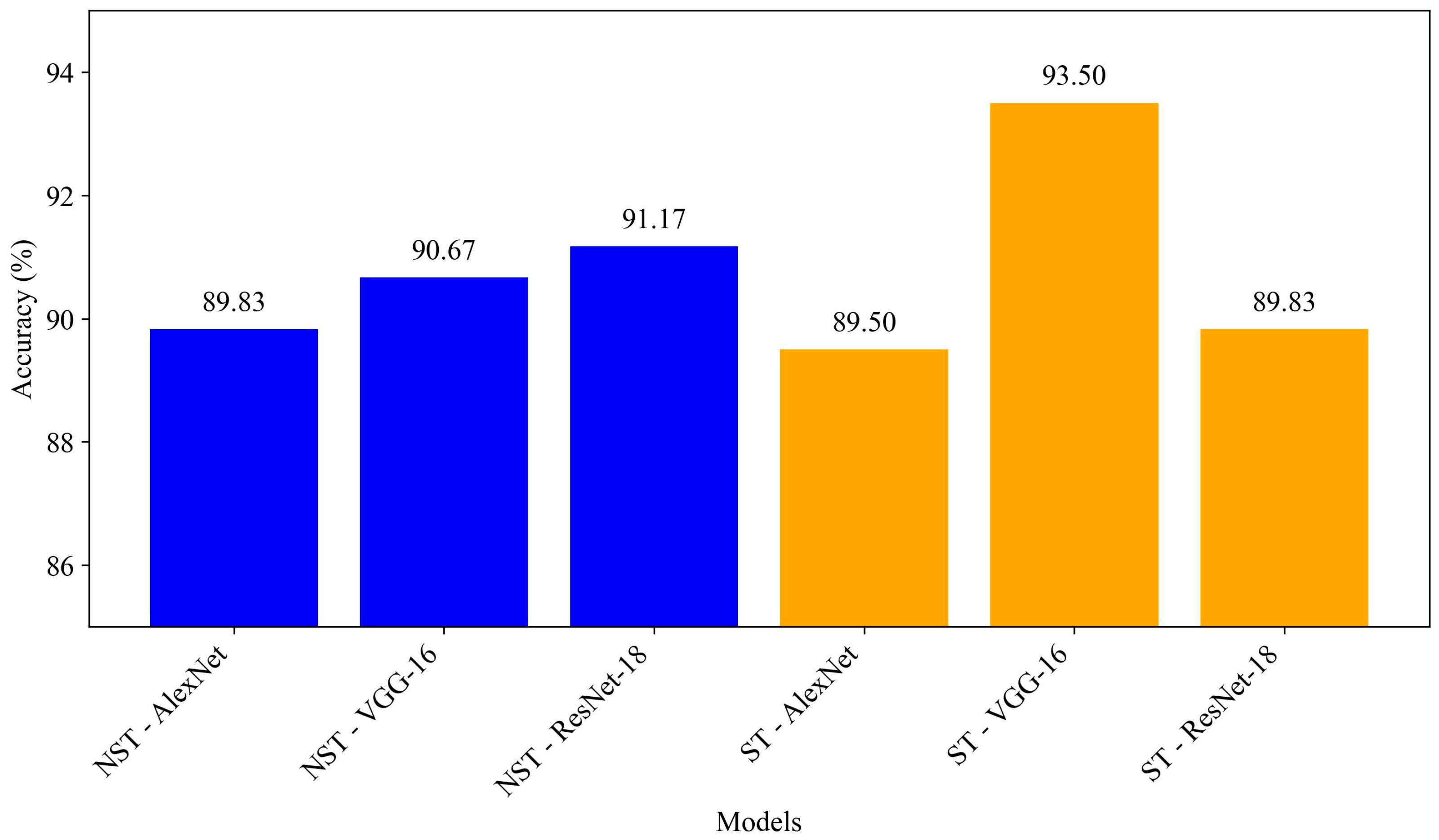
Among the models with the ST applied, VGG-16 demonstrates by far the best performance by analyzing Table 5. It leads this group with a precision of 93.68%, recall of 93.50%, F1-score of 93.49%, and accuracy of 93.50%, while also achieving the highest values in specificity (96.67%) and C2 (90.33%) metrics. ST-AlexNet delivers a mid-level performance with precision (90.05%), recall (89.50%), and accuracy (89.50%); although it achieves a strong specificity of 95.33%, it ties with ResNet-18 at a lower C2 score of 83.67%. ST-ResNet-18 exhibits the weakest performance in this group, lagging behind the others with precision (90.26%), recall (89.83%), F1-score (89.81%), and accuracy (89.83%), though it still provides an acceptable specificity of 95.00%. It is evident that the ST significantly improves VGG-16, while it has a negative impact on ResNet-18 and keeps AlexNet at a moderate level. In this group, ST-VGG-16 is clearly the most successful model.
When evaluating the Normal and Shearlet models together, it is observed that ST-VGG-16 achieved the highest performance in the overall comparison with an accuracy of 93.50%, while NST-ResNet-18 ranked second with 91.17% accuracy. Additionally, the ST improved the performance of VGG-16, whereas it had a different effect on ResNet-18.
In Figure 5, the accuracy results obtained by applying the No ST (NST) and ST to individual CNN models are presented. The bar chart compares the performance scores of AlexNet, VGG-16, and ResNet-18 under NST and ST conditions. The ST significantly improves VGG-16′s performance (93.50% vs. 90.67%) but has little to no effect on ResNet-18 (both 89.83%) and slightly reduces AlexNet’s performance (89.50% vs. 89.83%). Overall, ST-VGG-16 achieves the highest score, indicating that the ST is most beneficial for this model, while its impact on the others is minimal or slightly negative.

3.2. Hybrid Models

Performances with Optimization Techniques

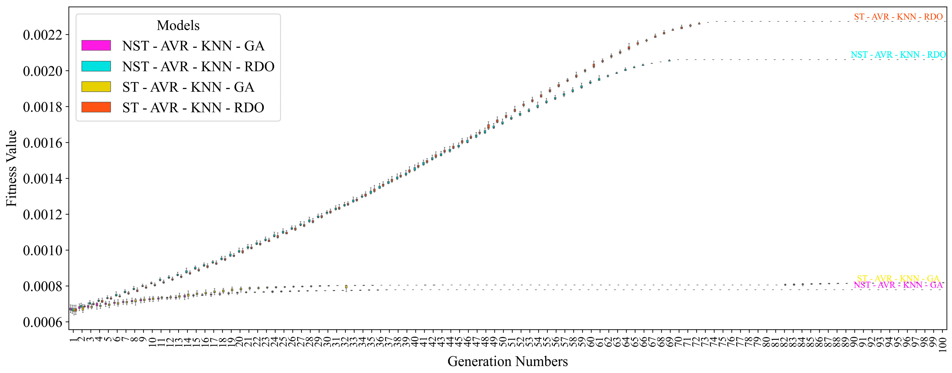
In this section, the most suitable features among those extracted from AlexNet, VGG-16, and ResNet-18 (AVR) models have been identified using GA and RDO approaches. Additionally, the impact of applying ST has been examined in this context. Figure 6 illustrates the variation in fitness value based on whether optimization approaches include ST. The fitness value is evaluated in terms of maximizing the recall value while minimizing the number of selected features. In this context, a higher fitness value indicates a greater likelihood of obtaining a high-performance model. Upon examining the graph, it is observed that the RDO approach produces higher fitness values compared to the GA approach. Furthermore, when the ST approach is applied, it is evident that higher fitness values emerge as generations progress, compared to cases where ST is not used. Consequently, it can be concluded that both RDO and ST approaches enhance performance relative to scenarios where neither is employed.
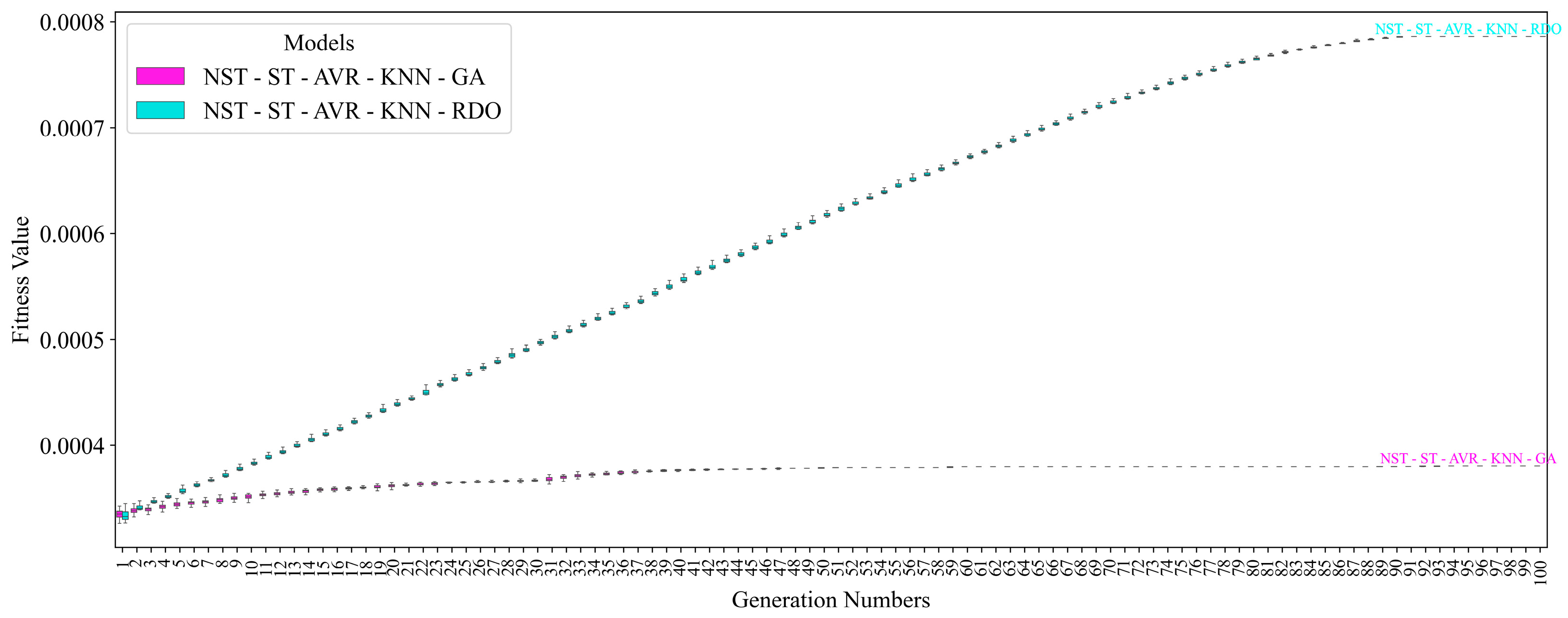
The features obtained using CNN approaches, from data with ST and NST, have been selected using GA and RDO methods. These results are presented in Figure 7. Similarly, it has been observed that the RDO approach outperforms GA, as evidenced by achieving higher fitness values. This difference becomes increasingly apparent as the number of generations increases.
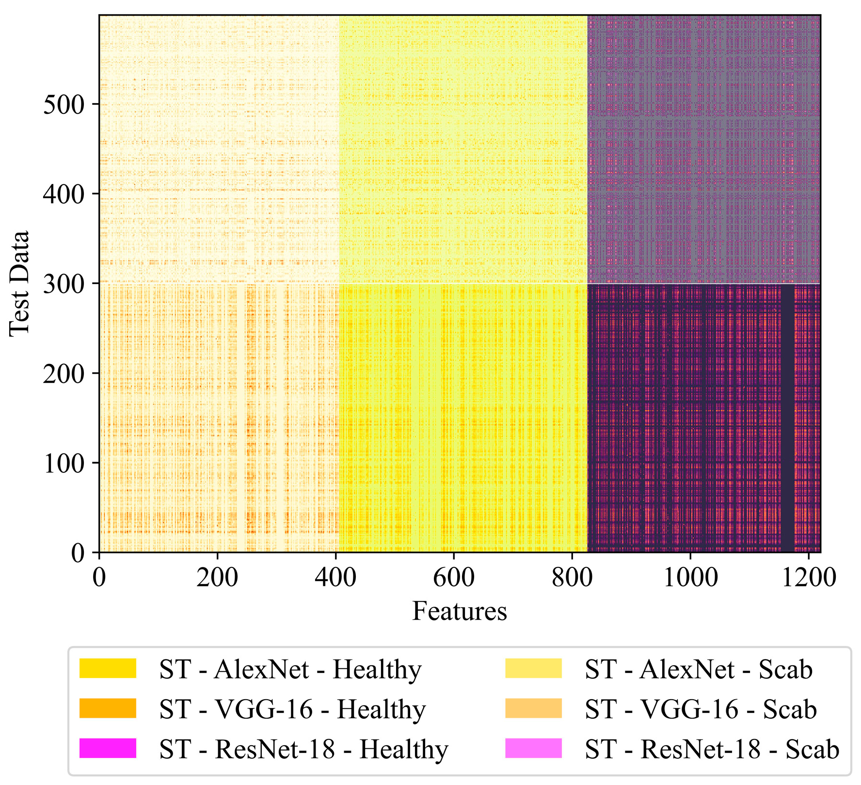
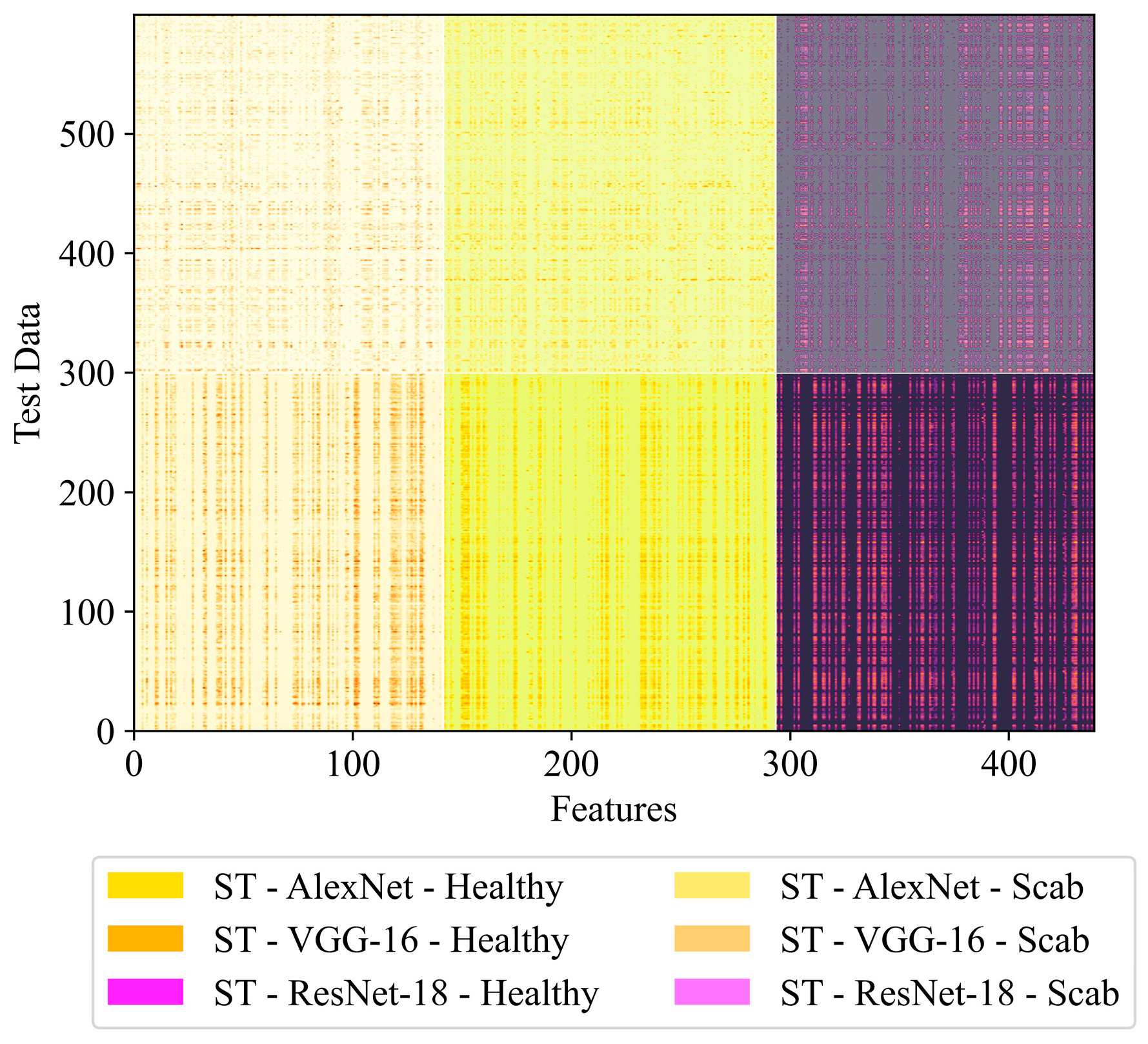
The features obtained as a result of all processes are presented as shown in Table 6 to indicate which CNN approach they are selected from. When examining NST-AVR-KNN-GA, it is observed that, without ST applied, GA selects a high number of features from normal data. This indicates that GA retains more features. In the case of NST-AVR-KNN-RDO, RDO selects significantly fewer features from the same normal data compared to GA (1284 > 485), demonstrating that RDO is more selective and efficient. For the ST-AVR-KNN-GA model, GA selects a high number of features from ST-applied data as well. When compared to the result of GA with normal data (1284), it is evident that ST slightly reduces the number of features (1284 > 1221). Upon analyzing ST-AVR-KNN-RDO, RDO selects far fewer features from ST data compared to GA (1221 > 440). The combination of ST and RDO dramatically reduces the number of features.
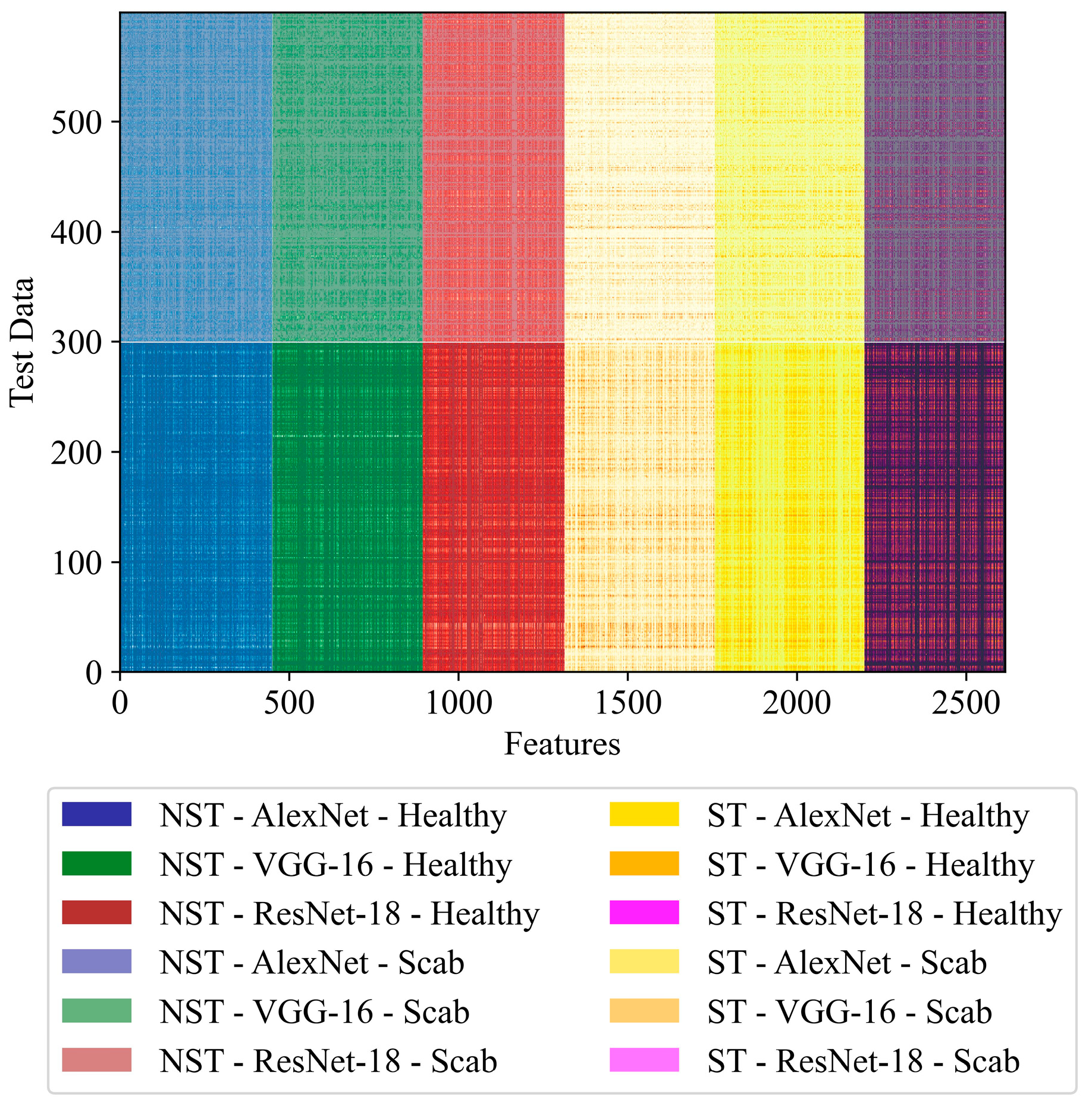
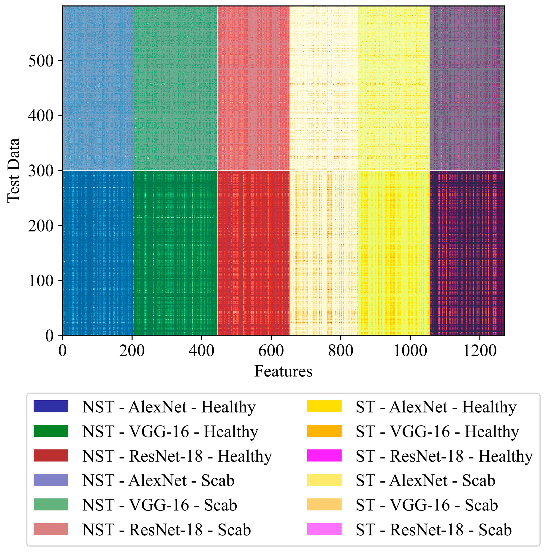
When evaluating the NST-ST-AVR-KNN-GA model, it is seen that when both normal and ST data are combined, GA results in a very high number of features. This suggests that GA retains a large number of features from both data types and is less selective. For NST-ST-AVR-KNN-RDO, RDO reduces the number of features by more than half compared to GA (2616 > 1272). Even in the mixed dataset, RDO’s efficiency stands out.
RDO selects fewer features in every case compared to GA, offering a more efficient optimization. ST plays a significant role in reducing the number of features, particularly when combined with RDO (440), yielding the most compact results. In the mixed dataset, while GA results in 2616 features, RDO reduces this to 1272, proving its superiority in both performance and efficiency. These findings demonstrate that the combination of RDO and ST is a powerful strategy for creating compact models with high performance potential.
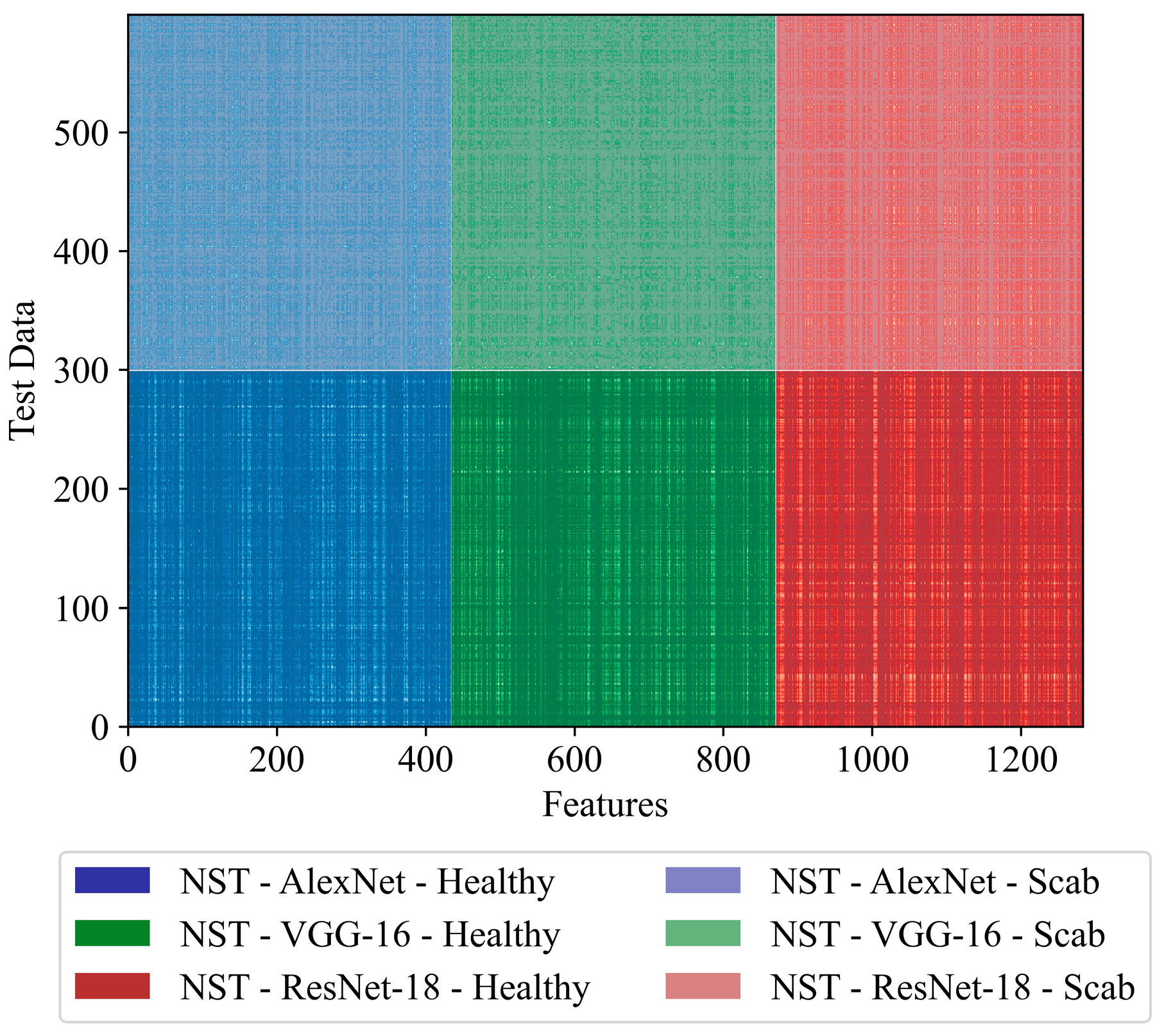
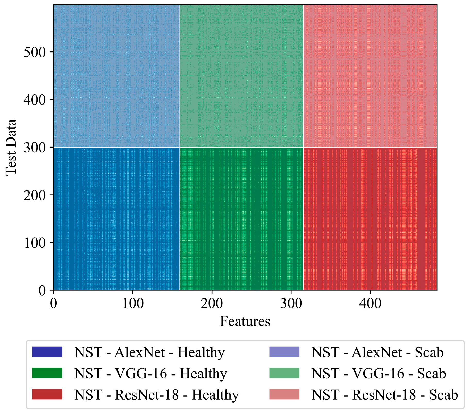
The distribution of features obtained and selected using AVR for the test data with the approaches NST-AVR-KNN-GA, NST-AVR-KNN-RDO, ST-AVR-KNN-GA, ST-AVR-KNN-RDO, NST-ST-AVR-KNN-GA, and NST-ST-AVR-KNN-RDO is also presented in Figure 8, Figure 9, Figure 10, Figure 11, Figure 12 and Figure 13.
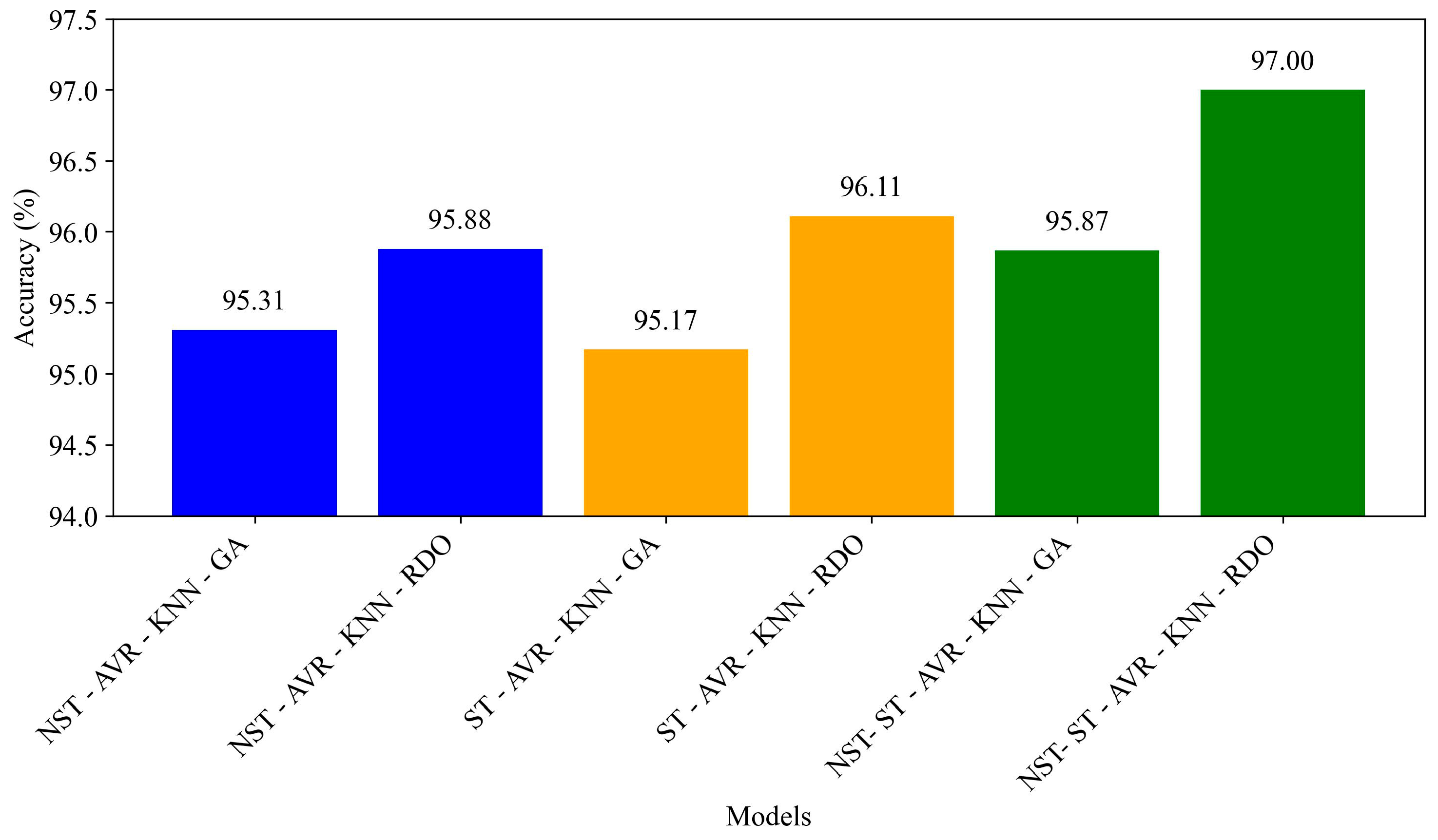
The performance metrics corresponding to the test data obtained as a result of 20 repeated training iterations are provided in Table 7. Figure 14, on the other hand, presents the accuracy values for hybrid models. All models exhibit high performance across all metrics, with mean values generally exceeding 95%. This suggests that the models are robust and effective for the given task. The NST-ST-AVR-KNN-RDO model achieves the highest overall accuracy (97.00 ± 0.31), while ST-AVR-KNN-RDO follows closely with 96.11 ± 0.29. The lowest accuracy is observed in ST-AVR-KNN-GA (95.17 ± 0.43). Standard deviations are relatively low (ranging from ±0.18 to ±0.63), indicating consistent performance across the 20 training iterations. The NST-ST-AVR-KNN-GA model has the smallest standard deviation for accuracy (±0.19) and F1-score (±0.18), suggesting it is the most stable. Models optimized with RDO consistently outperform their GA counterparts across all conditions (NST, ST, and NST-ST) in terms of accuracy, precision, F1-score, and specificity. This suggests that RDO might be a more effective optimization technique for apple scab classification.
In Figure 15, the ROC comparison of six single deep-learning models shows that all achieve very high performance (AUC (Area Under the Curve) 0.944–0.955). NST-AlexNet performs best (0.955), closely followed by ST-AlexNet (0.953) and NST-VGG-16 (0.952). Although ResNet-18 variants score slightly lower (0.944–0.948), they still provide strong discrimination. Overall, AlexNet-based models—especially the NST version—outperform VGG-16 and ResNet-18 by a small margin, and all single models perform near-perfectly.
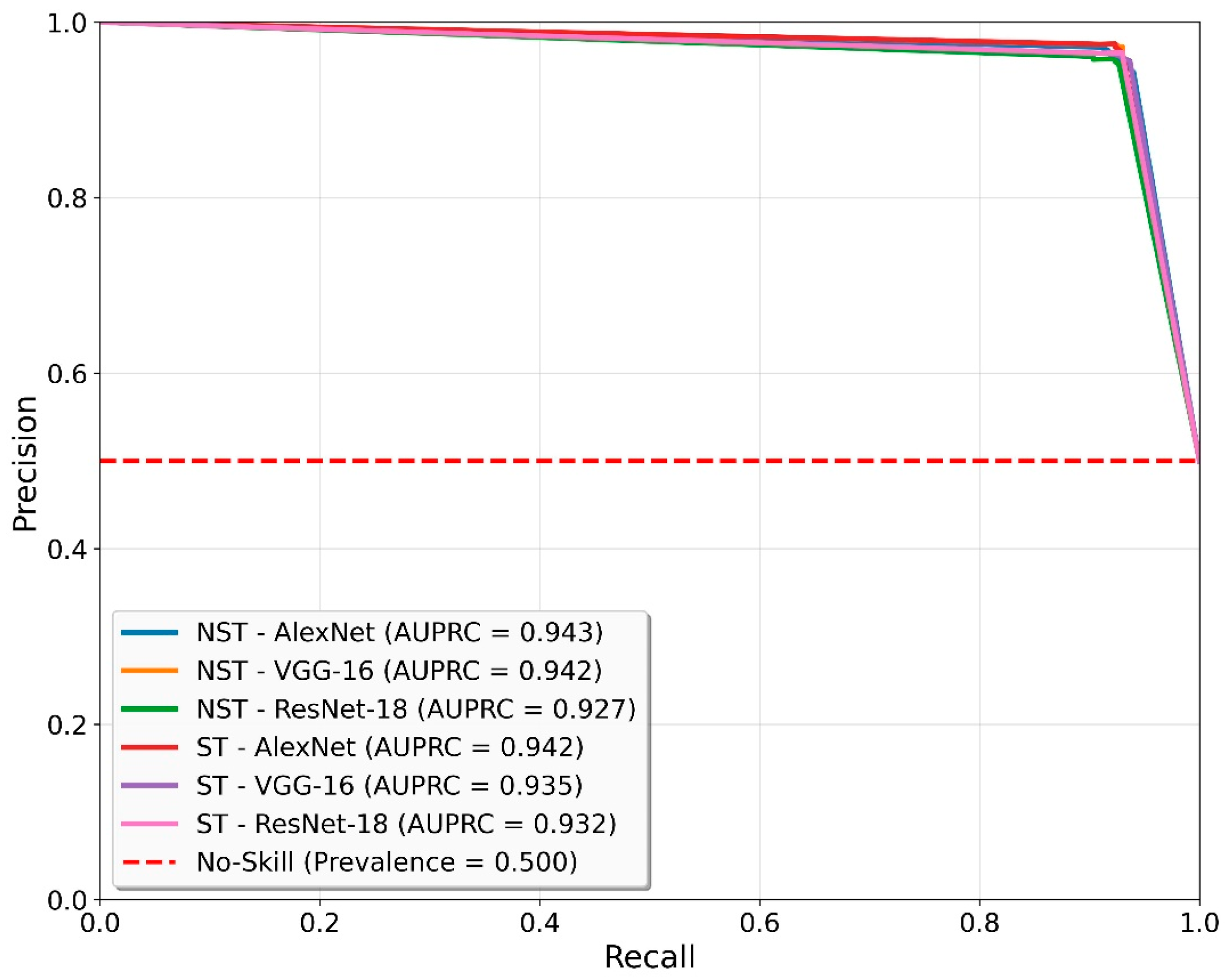
In Figure 16, the Precision–Recall curves show that all six single models perform very strongly, with AUPRC (Area Under the Precision–Recall Curve) scores ranging from 0.927 to 0.943. The best result comes from NST-AlexNet (0.943), followed closely by NST-VGG-16 and ST-AlexNet (both ≈0.942). Although the ResNet-18 models score slightly lower, they still achieve high precision across almost all recall levels. Overall, every model stays well above the no-skill baseline, indicating consistently strong class-separation performance.
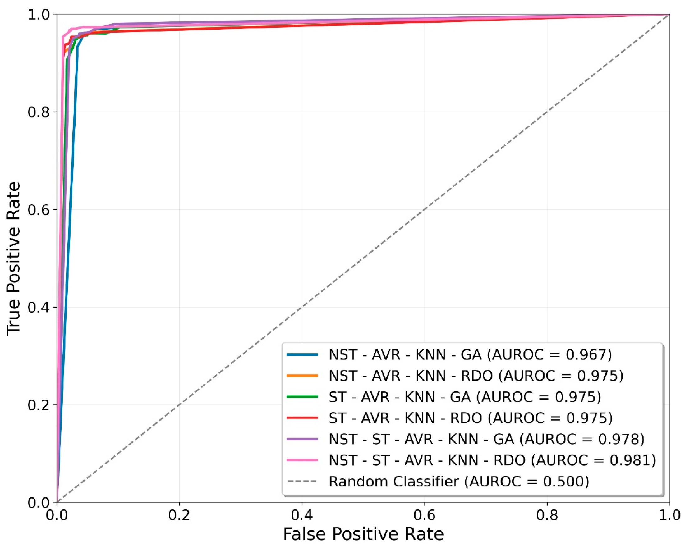
In Figure 17, the ROC comparison shows that all hybrid models achieve very high AUROC values, ranging from 0.967 to 0.981, indicating excellent discrimination. The weakest performer is NST-AVR-KNN-GA (0.967), while the strongest is NST-ST-AVR-KNN-RDO (0.981). Most models cluster tightly around 0.975–0.981, meaning their performance is almost identical and near-perfect. All curves stay far above the random classifier line, showing that combining feature extraction (NST/ST + AVR) with KNN and optimization (GA/RDO) leads to consistently superior results, especially for the RDO-based model.
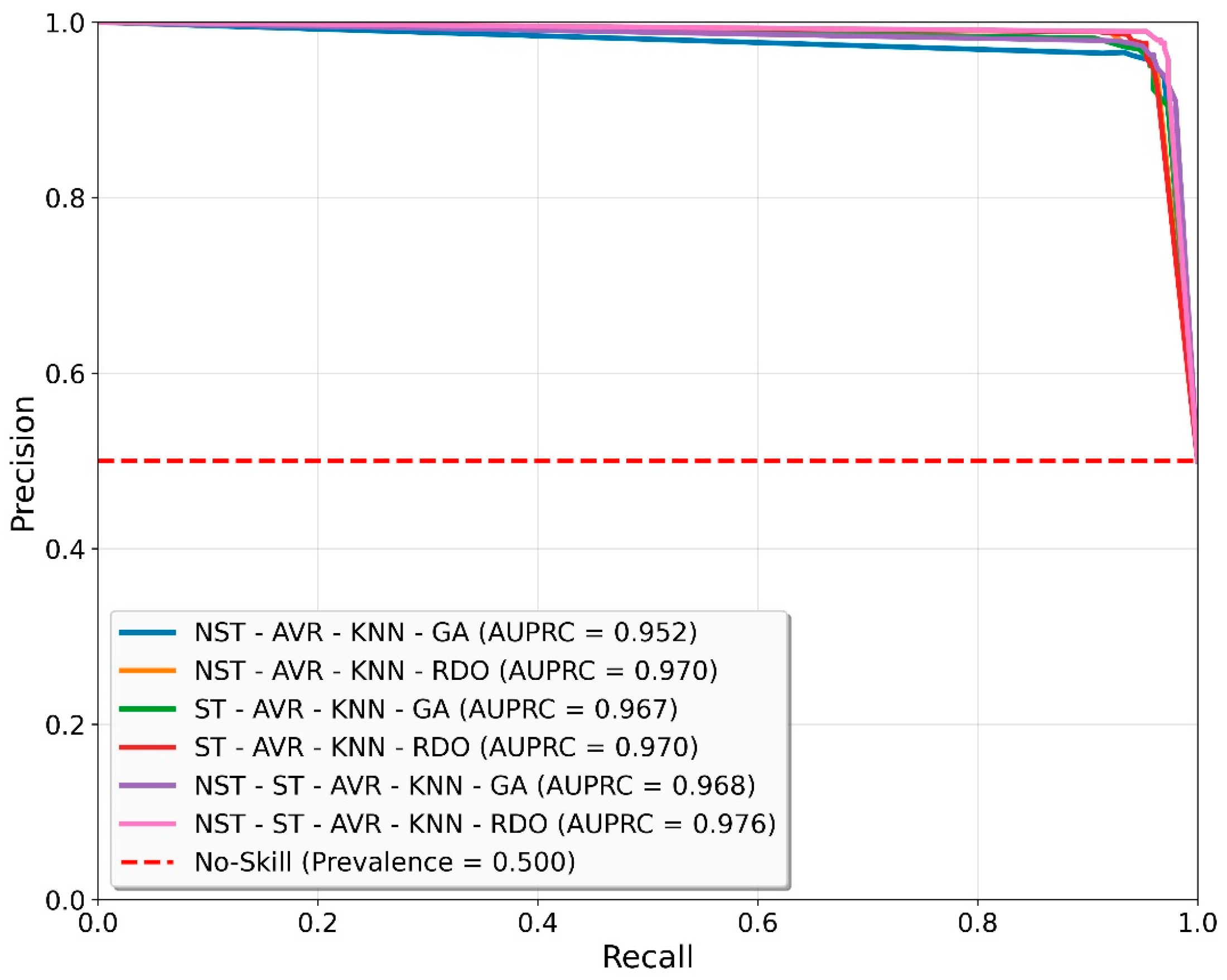
In Figure 18, the Precision–Recall curves show that all hybrid models achieve very strong performance, with AUPRC values between 0.952 and 0.976. The best performer is NST-ST-AVR-KNN-RDO (0.976), while NST-AVR-KNN-GA (0.952) is the weakest but still well above the no-skill baseline. Overall, RDO-based models consistently outperform GA-based ones, and all curves remain far above the no-skill line, indicating excellent precision across nearly all recall levels.
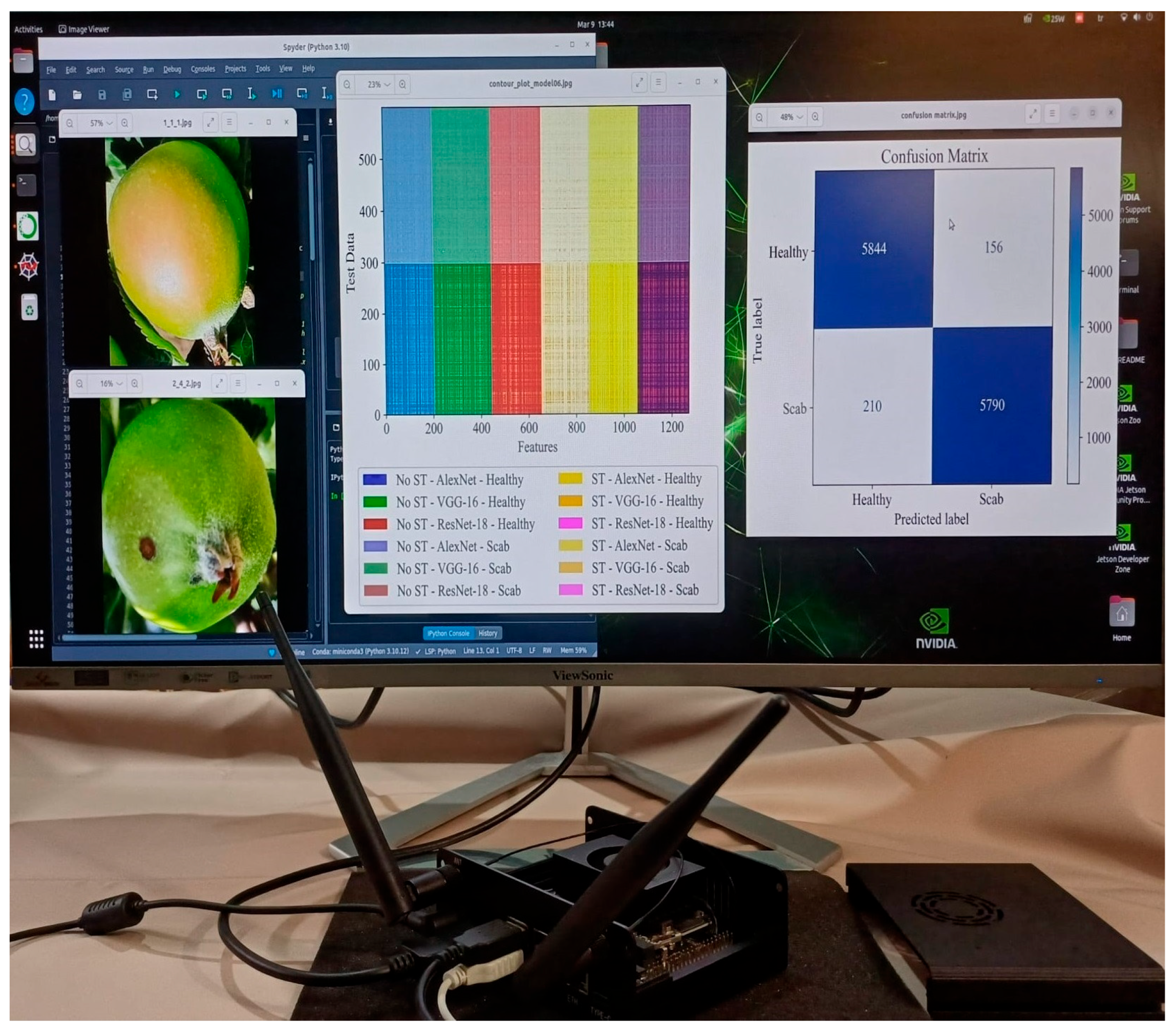
In addition, the testing process is conducted as on the Jetson Orin Nano platform, as shown in Figure 19, ensuring the development of a platform-independent model capable of consistent performance across diverse hardware environments.
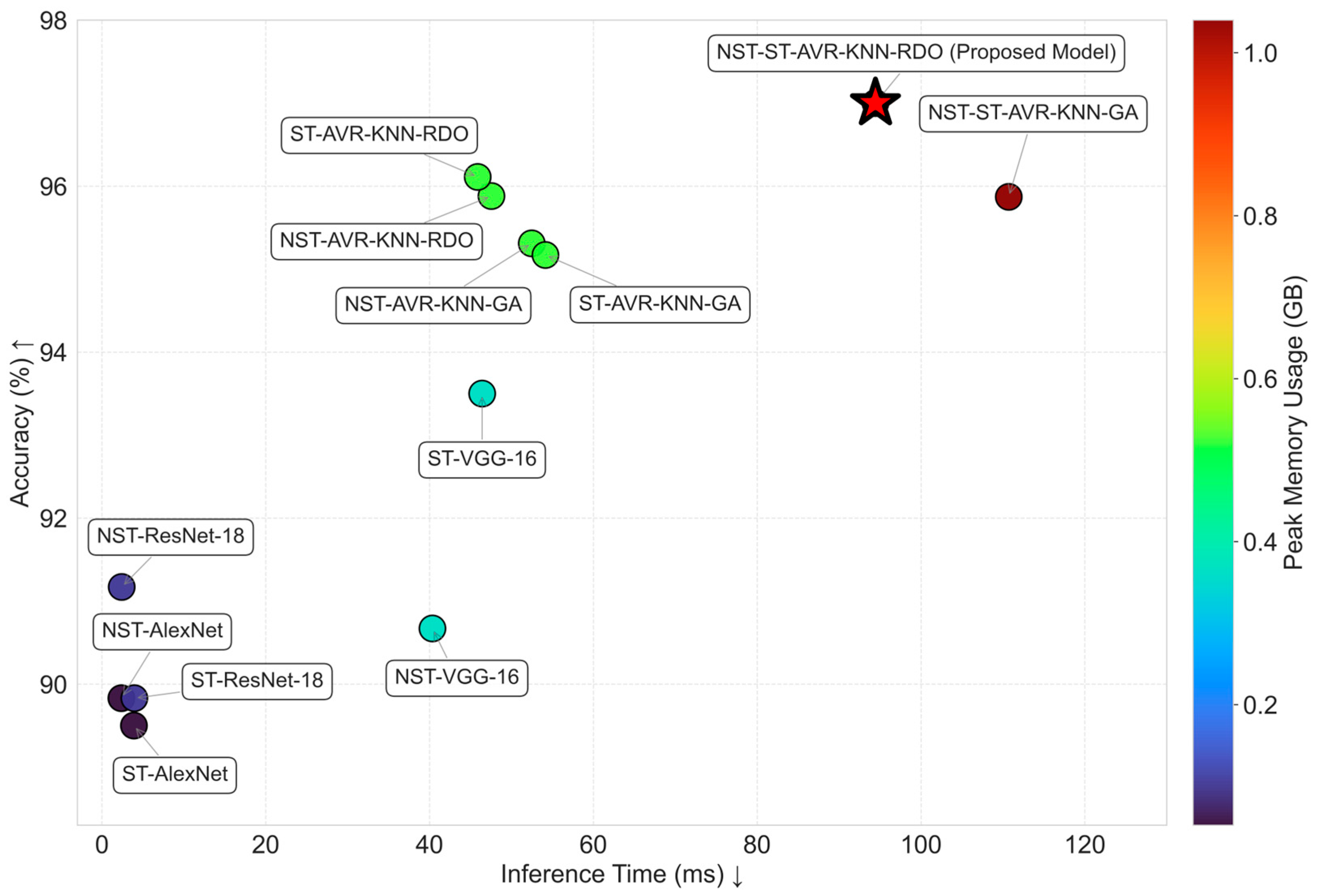
The results in Table 8 and Figure 20 clearly demonstrate the superiority of the proposed hybrid approaches over conventional deep learning architectures. Among standalone CNNs, ResNet-18 achieves the highest accuracy (91.17%) with the fastest inference time (~0.0024 s) on Jetson Orin Nano platform while maintaining moderate memory footprint similar to AlexNet. However, none of the pure CNN models exceed 93% accuracy. The proposed AVR + KNN-enhanced hybrid models significantly outperform all baseline CNNs, reaching accuracies between 95.17% and 97.00%. The best performance (97.00%) is obtained with the combined NST-ST-AVR-KNN-RDO model, which improves accuracy by +3.5 percentage points over the strongest baseline (ST-VGG-16, 93.50%) while keeping inference time at an acceptable 0.09444 s for real time application. Although the hybrid models increase memory usage by 2–3× (532–1064 MB) and inference time by 15–20× compared to lightweight CNNs, the substantial accuracy gain of ~6–7 points justify these trade-offs for most practical applications. Combining both NST and ST features with AVR-KNN and RDO optimization yields the overall best accuracy-performance balance.
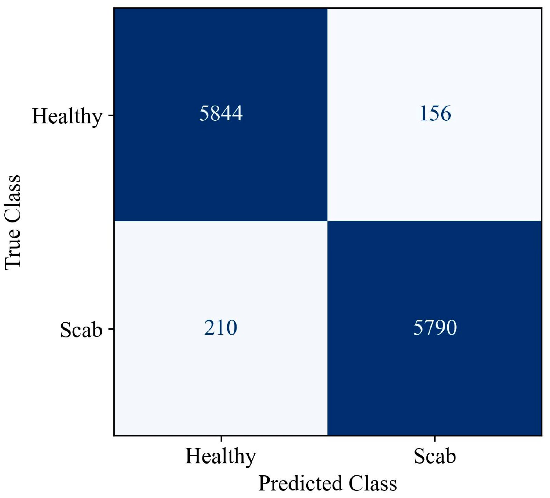
The confusion matrix, as shown in Figure 21, reflects an excellent classification model with approximately 97% accuracy and balanced performance across the Healthy and Scab classes. It likely corresponds to one of the top-performing configurations from the previous table, specifically the NST-ST-AVR-KNN-RDO model.
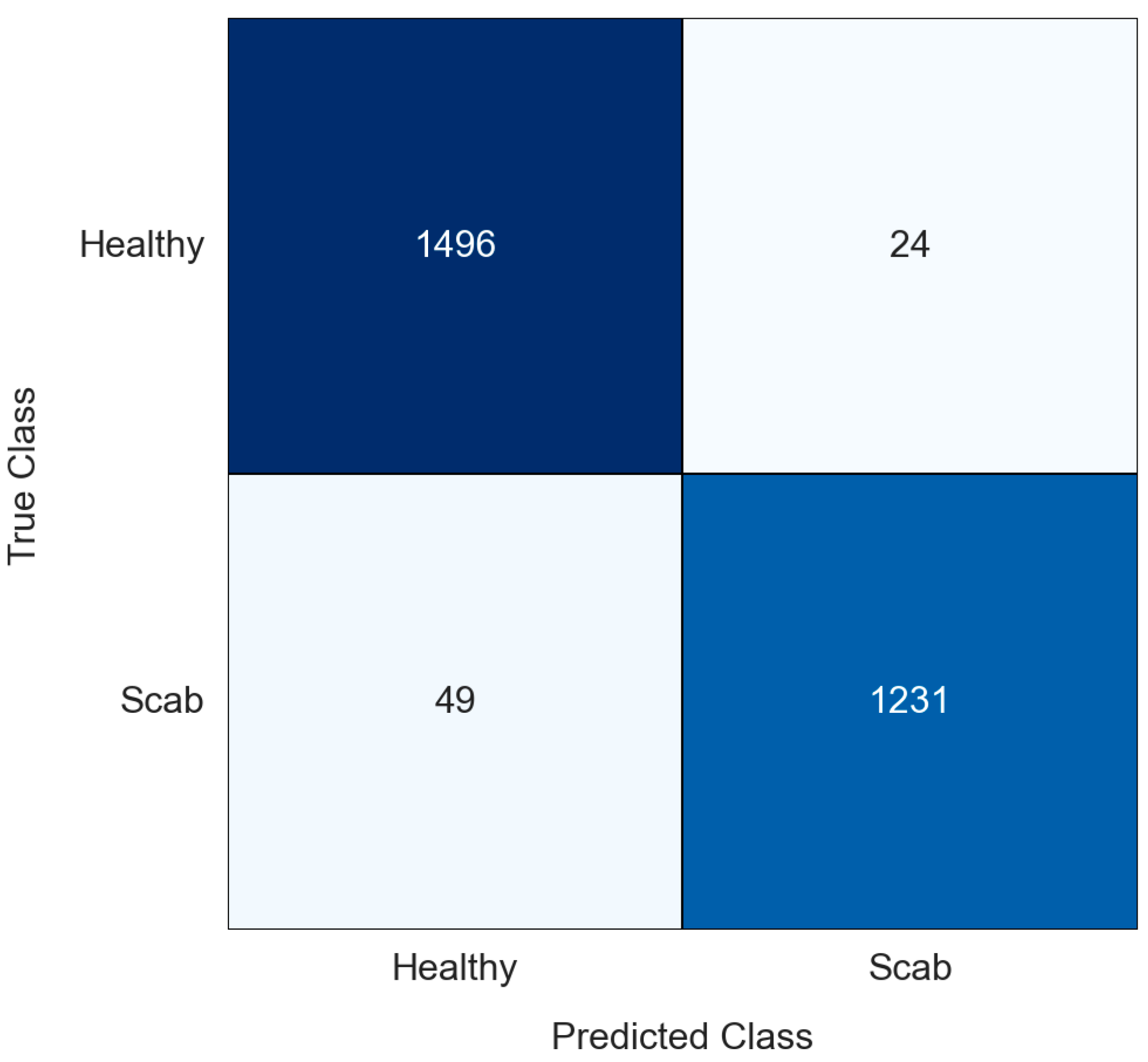
The performance of the proposed framework is systematically evaluated under varying levels of Gaussian noise (σ = 0.01, 0.03, 0.05, 0.1) and Salt & Pepper noise (densities 1%, 3%, 5%, 10%) intentionally injected into the test images. The results clearly demonstrate that the proposed method retains high classification accuracy even under severe noise conditions. Confusion matrices of the proposed NST-ST-AVR-KNN-RDO model under various noise conditions (including 140 noisy samples in the augmented dataset) are presented in Figure 22. These matrices clearly demonstrate the model’s exceptional robustness, maintaining outstanding classification performance even in the presence of significant noise, as evidenced by the impressive 97.39% accuracy achieved across 20 repeated experiments.

4. Conclusions and Future Research

Early diagnosis of apple disease using automated systems is becoming an increasingly important and critical topic in modern agricultural practices to minimize yield losses and support sustainable production. In particular, machine learning and deep learning approaches enable more detailed and accurate detection in the early stages of the diagnosis process. As the symptoms of apple scab disease in its early stages consist of small, easily overlooked spots, hybrid approaches have become prominent in this field. In this article, a new apple disease recognition system is developed, enhancing performance through a two-dimensional signal processing approach, feature analysis based on deep learning, and a meta-heuristic optimization approach. In the proposed model, images processed with ST are first classified to improve the classification performance of CNN architectures such as AlexNet, VGG-16, and ResNet-18. Subsequently, the optimization process is carried out using the RDO approach for features extracted from both transformed and untransformed images. At this stage, binary classification is performed using the KNN classifier. The model’s performance is compared with that of other models in the literature using various metrics. As is shown in Table 9 and Figure 23, the proposed method outperforms current single and hybrid approaches. Although the dataset contained an equal number of samples from each class, the classification performance for both healthy and scab apples is found to be similar, indicating the robustness of the model. It is evident that the resulting model will enable farmers to obtain more reliable results in the early diagnosis of diseases, thereby contributing to increased agricultural productivity. In future studies, a comprehensive dataset could be created using data from different geographical regions and climatic conditions. Additionally, integrating the system into mobile platforms could enhance early diagnosis efforts. Beyond this, integration with mobile platforms could facilitate the creation of datasets combining multi-sensor data. All these efforts will help prevent unnecessary pesticide use and increase efficiency in farmers’ operations.

Funding

This research received no external funding.

Data Availability Statement

Data is contained within the article.

Conflicts of Interest

The author declares no conflicts of interest.

References

  1. Berry, E.; Dernini, S.; Burlingame, B.; Meybeck, A.; Conforti, P. Food security and sustainability: Can one exist without the other? Public Health Nutr. 2015, 18, 2293–2302. [Google Scholar] [CrossRef]
  2. Nagarajan, S.; Nagarajan, S. Abiotic tolerance and crop improvement. In Abiotic Stress Adaptation in Plants: Physiological, Molecular and Genomic Foundation; Springer: Dordrecht, The Netherlands, 2010; pp. 1–11. [Google Scholar]
  3. Simsek, M.; Ergun, M.; Ozbay, N. Development of Fruit Sapling Cultivation in Bingöl. In Proceedings of the 3rd Bingöl Symposium, Bingöl, Türkiye, 17–19 September 2010; pp. 261–265. [Google Scholar]
  4. Pereira, L.S.; Oweis, T.; Zairi, A. Irrigation management under water scarcity. Agric. Water Manag. 2002, 57, 175–206. [Google Scholar] [CrossRef]
  5. Russell, S.D. Double fertilization. Int. Rev. Cytol. 1992, 140, 357–388. [Google Scholar]
  6. Kolmanič, S.; Strnad, D.; Kohek, Š.; Benes, B.; Hirst, P.; Žalik, B. An algorithm for automatic dormant tree pruning. Appl. Soft Comput. 2021, 99, 106931. [Google Scholar] [CrossRef]
  7. Metzidakis, I.; Martinez-Vilela, A.; Nieto, G.C.; Basso, B. Intensive olive orchards on sloping land: Good water and pest management are essential. J. Environ. Manag. 2008, 89, 120–128. [Google Scholar] [CrossRef]
  8. FAO. Agricultural Production Statistics. 2000–2020; FAOSTAT Analytical Brief Series 41; FAO: Rome, Italy, 2022. [Google Scholar]
  9. Rouš, R.; Peller, J.; Polder, G.; Hageraats, S.; Ruigrok, T.; Blok, P.M. Apple scab detection in orchards using deep learning on colour and multispectral images. arXiv 2023, arXiv:2302.08818. [Google Scholar] [CrossRef]
  10. Zhong, Y.; Zhao, M. Research on deep learning in apple leaf disease recognition. Comput. Electron. Agric. 2020, 168, 105146. [Google Scholar] [CrossRef]
  11. Bowen, J.; Mesarich, C.; Bus, V.; Beresford, R.; Plummer, K.; Templeton, M. Venturia inaequalis: The causal agent of apple scab. Mol. Plant Pathol. 2011, 12, 105–122. [Google Scholar] [CrossRef]
  12. Pearson, R. Suppression of Cedar Apple Rust Pycnia on Apple Leaves Following Postinfection Applications of Fenarimol and Triforine. Phytopathology 1978, 68, 1805. [Google Scholar] [CrossRef]
  13. Abbasi, N.; Shahid, M.; Naz, F.; And, G. Surveillance and characterization of Botryosphaeria obtusa causing frogeye leaf spot of Apple in District Quetta. Mycopathologia 2020, 16, 111–115. [Google Scholar]
  14. Brown-Rytlewski, D.; Mcmanus, P. Virulence of Botryosphaeria dothidea and Botryosphaeria obtusa on Apple and Management of Stem Cankers with Fungicides. Plant Dis. 2020, 84, 1031–1037. [Google Scholar] [CrossRef] [PubMed]
  15. MacHardy, W.E.; Gadoury, D.M.; Gessler, C. Parasitic and biological fitness of Venturia inaequalis: Relationship to disease management strategies. Plant Dis. 2001, 85, 1036–1051. [Google Scholar] [CrossRef] [PubMed]
  16. Cuthbertson, A.G.S.; Murchie, A.K. The impact of fungicides to control apple scab (Venturia inaequalis) on the predatory mite Anystis baccarum and its prey Aculus schlechtendali (apple rust mite) in Northern Ireland Bramley orchards. Crop Prot. 2003, 22, 1125–1130. [Google Scholar] [CrossRef]
  17. Moura, L.; Pinto, R.; Rodrigues, R.; Brito, L.; Rego, R.; Valín, M.; Mariz-Ponte, N.; Santos, C.; Mourão, I. Effect of Photo-Selective Nets on Yield, Fruit Quality and Psa Disease Progression in a ‘Hayward’ Kiwifruit Orchard. Horticulturaei 2022, 8, 1062. [Google Scholar] [CrossRef]
  18. Kodors, S.; Lacis, G.; Sokolova, O.; Zhukovs, V.; Apeinans, I.; Bartulsons, T. Apple scab detection using CNN and Transfer Learning. Agron. Res. 2021, 19, 507–519. [Google Scholar]
  19. Kodors, S.; Lācis, G.; Moročko-Bičevska, I.; Zarembo, I.; Sokolova, O.; Bartulsons, T.; Apeinâns, I.; Žukovs, V. Apple Scab Detection in the Early Stage of Disease Using a Convolutional Neural Network. Proc. Latv. Acad. Sci. 2022, 76, 482–487. [Google Scholar] [CrossRef]
  20. Vishnoi, V.K.; Kumar, K.; Kumar, B.; Mohan, S.; Khan, A.A. Detection of Apple Plant Diseases Using Leaf Images Through Convolutional Neural Network. IEEE Access 2022, 11, 6594–6609. [Google Scholar] [CrossRef]
  21. Karpyshev, P.; Ilin, V.; Kalinov, I.; Petrovsky, A.; Tsetserukou, D. Autonomous mobile robot for apple plant disease detection based on cnn and multi-spectral vision system. In Proceedings of the 2021 IEEE/SICE International Symposium on System Integration (SII), Iwaki, Japan, 11–14 January 2021. [Google Scholar]
  22. Dubey, S.R.; Jalal, A.S. Apple disease classification using color, texture and shape features from images. Signal Image Video Process. 2016, 10, 819–826. [Google Scholar] [CrossRef]
  23. Raman, S.; Chougule, A.; Chamola, V. A low power consumption mobile based IoT framework for real-time classification and segmentation for apple disease. Microprocess. Microsyst. 2022, 94, 104656. [Google Scholar] [CrossRef]
  24. Singh, H.; Saxena, K.; Jaiswal, A.K. Apple disease classification built on deep learning. In Proceedings of the 2022 3rd International Conference on Intelligent Engineering and Management (ICIEM), London, UK, 27–29 April 2022. [Google Scholar]
  25. Patidar, A.; Chakravorty, A. Using Machine Learning to Identify Diseases and Perform Sorting in Apple Fruit. Int. J. Innov. Sci. Res. Technol. 2024, 9, 732–750. [Google Scholar] [CrossRef]
  26. Subha, V.; Kasturi, K. Structural Invariant Feature Segmentation Based Apple Fruit Disease Detection Using Deep Spectral Generative Adversarial Networks. SN Comput. Sci. 2024, 5, 635. [Google Scholar] [CrossRef]
  27. Van Dyk, D.; Meng, X. The Art of Data Augmentation. J. Comput. Graph. Stat. 2001, 10, 1–50. [Google Scholar] [CrossRef]
  28. Shon, H.S.; Batbaatar, E.; Cho, W.S.; Choi, S.G. Unsupervised pre-training of imbalanced data for identification of wafer map defect patterns. IEEE Access 2021, 9, 52352–52363. [Google Scholar] [CrossRef]
  29. Maslej-Krešňáková, V.; El Bouchefry, K.; Butka, P. Morphological classification of compact and extended radio galaxies using convolutional neural networks and data augmentation techniques. Mon. Not. R. Astron. Soc. 2021, 505, 1464–1475. [Google Scholar] [CrossRef]
  30. Liu, L.; Zhan, X.; Wu, R.; Guan, X.; Wang, Z.; Zhang, W.; Pilanci, M.; Wang, Y.; Luo, Z.; Li, G. Boost AI power: Data augmentation strategies with unlabeled data and conformal prediction, a case in alternative herbal medicine discrimination with electronic nose. IEEE Sens. J. 2021, 21, 22995–23005. [Google Scholar] [CrossRef]
  31. Shorten, C.; Khoshgoftaar, T. A survey on Image Data Augmentation for Deep Learning. J. Big Data 2019, 6, 60. [Google Scholar] [CrossRef]
  32. Wang, Y.; Huang, G.; Song, S.; Pan, X.; Xia, Y.; Wu, C. Regularizing Deep Networks with Semantic Data Augmentation. IEEE Trans. Pattern Anal. Mach. Intell. 2020, 44, 3733–3748. [Google Scholar] [CrossRef]
  33. Wang, K.; Fang, B.; Qian, J.; Yang, S.; Zhou, X.; Zhou, J. Perspective Transformation Data Augmentation for Object Detection. IEEE Access 2020, 8, 4935–4943. [Google Scholar] [CrossRef]
  34. Kim, S.; Lussi, R.; Qu, X.; Huang, F.; Kim, H. Reversible Data Hiding with Automatic Brightness Preserving Contrast Enhancement. IEEE Trans. Circuits Syst. Video Technol. 2019, 29, 2271–2284. [Google Scholar] [CrossRef]
  35. Cortés-Ciriano, I.; Bender, A. Improved Chemical Structure-Activity Modeling Through Data Augmentation. J. Chem. Inf. Model. 2015, 55, 2682–2692. [Google Scholar] [CrossRef]
  36. Xing, Y.; Xu, J.; Tan, J.; Li, D.; Zha, W. Deep CNN for removal of salt and pepper noise. IET Image Process. 2019, 13, 1550–1560. [Google Scholar] [CrossRef]
  37. Jia, S.; Ping, W.; Peiyi, J.; Hu, S. Research on data augmentation for image classification based on convolution neural networks. In Proceedings of the 2017 Chinese Automation Congress (CAC), Jinan, China, 20–22 October 2017; pp. 4165–4170. [Google Scholar]
  38. Easley, G.; Labate, D.; Lim, W. Sparse directional image representations using the discrete shearlet transform. Appl. Comput. Harmon. Anal. 2008, 25, 25–46. [Google Scholar] [CrossRef]
  39. Yi, S.; Labate, D.; Easley, G.; Krim, H. A Shearlet Approach to Edge Analysis and Detection. IEEE Trans. Image Process. 2009, 18, 929–941. [Google Scholar] [CrossRef] [PubMed]
  40. Zhang, C.; Baan, M. Multicomponent microseismic data denoising by 3D shearlet transform. Geophysics 2018, 83, A45–A51. [Google Scholar] [CrossRef]
  41. Negi, P.; Labate, D. 3-D Discrete Shearlet Transform and Video Processing. IEEE Trans. Image Process. 2012, 21, 2944–2954. [Google Scholar] [CrossRef]
  42. Vidyasagar, K.; Kumar, R.; Sai, G.; Ruchita, M.; Saikia, M. Signal to Image Conversion and Convolutional Neural Networks for Physiological Signal Processing: A Review. IEEE Access 2024, 12, 66726–66764. [Google Scholar] [CrossRef]
  43. Kwon, H.; Lee, J. AdvGuard: Fortifying Deep Neural Networks Against Optimized Adversarial Example Attack. IEEE Access 2024, 12, 5345–5356. [Google Scholar] [CrossRef]
  44. Zoughi, T.; Homayounpour, M.; Deypir, M. Adaptive windows multiple deep residual networks for speech recognition. Expert Syst. Appl. 2020, 139, 112840. [Google Scholar] [CrossRef]
  45. Kaur, T.; Gandhi, T. Deep convolutional neural networks with transfer learning for automated brain image classification. Mach. Vis. Appl. 2020, 31, 20. [Google Scholar] [CrossRef]
  46. Chen, S.; Ge, H.; Li, H.; Sun, Y.; Qian, X. Hierarchical deep convolution neural networks based on transfer learning for transformer rectifier unit fault diagnosis. Measurement 2021, 167, 108257. [Google Scholar] [CrossRef]
  47. Krizhevsky, A.; Sutskever, I.; Hinton, G.E. Imagenet classification with deep convolutional neural networks. In Advances in Neural Information Processing Systems 25; Curran Associates, Inc.: Red Hook, NY, USA, 2012. [Google Scholar]
  48. Simonyan, K.; Zisserman, A. Very deep convolutional networks for large-scale image recognition. arXiv 2014, arXiv:1409.1556. [Google Scholar]
  49. He, K.; Zhang, X.; Ren, S.; Sun, J. Deep residual learning for image recognition. In Proceedings of the IEEE Conference on Computer Vision and Pattern Recognition, Las Vegas, NV, USA, 27–30 June 2016. [Google Scholar]
  50. Fathollahi-Fard, A.M.; Hajiaghaei-Keshteli, M.; Tavakkoli-Moghaddam, R. Red deer algorithm (RDA): A new nature-inspired meta-heuristic. Soft Comput. 2020, 24, 14637–14665. [Google Scholar] [CrossRef]
  51. Juneja, S.; Kaur, K.; Singh, H.; Richa. Bio Inspired Meta Heuristic Approach based on Red Deer in WSN. In Proceedings of the 2022 7th International Conference on Communication and Electronics Systems (ICCES), Coimbatore, India, 22–24 June 2022. [Google Scholar]
  52. Fathollahi-Fard, A.M.; Niaz Azari, M.; Hajiaghaei-Keshteli, M. An improved red deer algorithm for addressing a direct current brushless motor design problem. Sci. Iran. 2021, 28, 1750–1764. [Google Scholar]
  53. Ganesh, N.; Jayalakshmi, S.; Narayanan, R.; Mahdal, M.; Zawbaa, H.; Mohamed, A. Gated Deep Reinforcement Learning with Red Deer Optimization for Medical Image Classification. IEEE Access 2023, 11, 58982–58993. [Google Scholar] [CrossRef]
  54. Goudarzi, P.; Rahmani, A.; Mosleh, M. A mathematical optimization model using red deer algorithm for resource discovery in CloudIoT. Trans. Emerg. Telecommun. Technol. 2022, 33, e4646. [Google Scholar] [CrossRef]
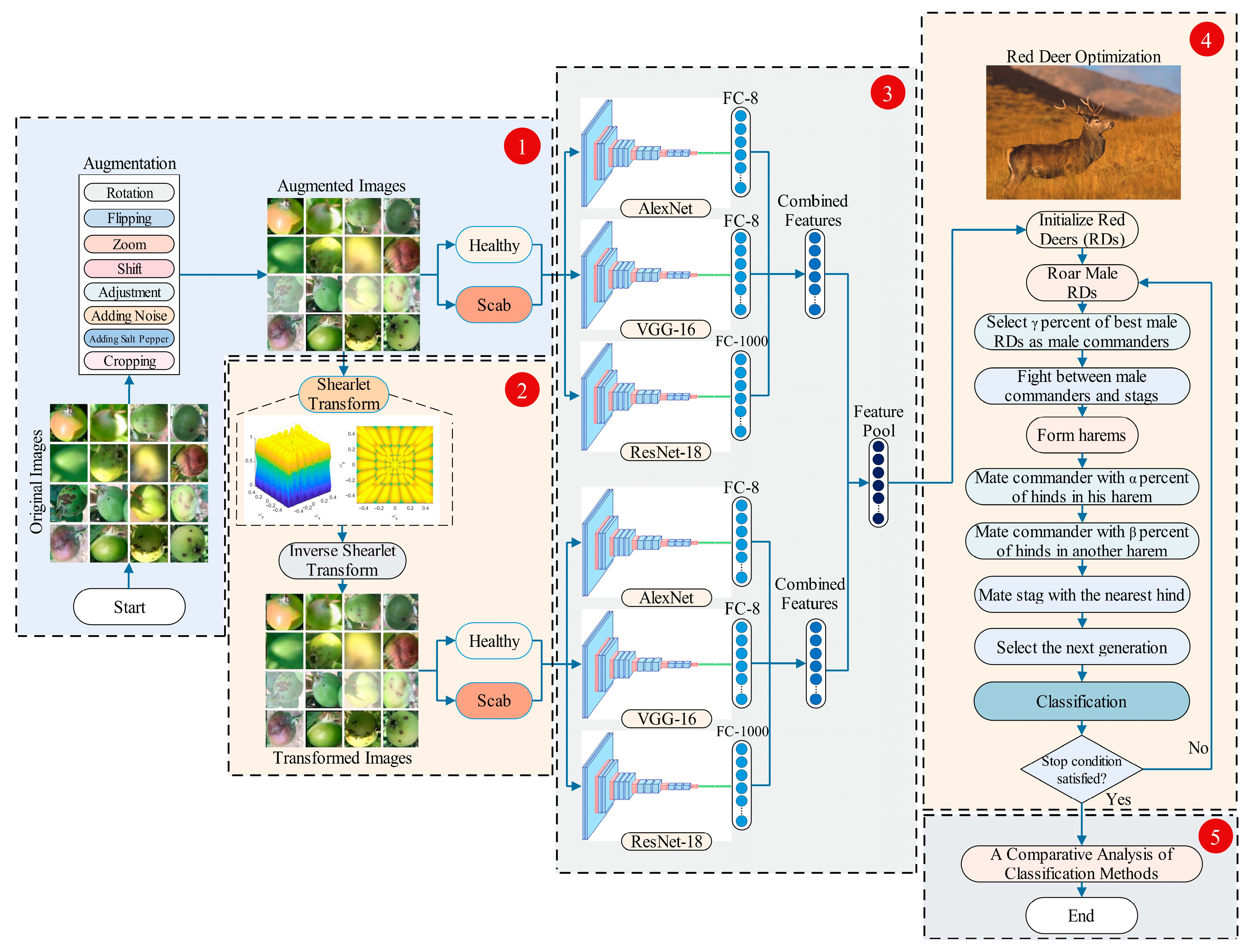
Figure 1. Block diagram of proposed framework for apple scab classification model.
Electronics 14 04678 g001
Figure 2. Data collection locations shown on the map [18].
Electronics 14 04678 g002
Figure 3. Resolution distributions of healthy and scab apple images.
Electronics 14 04678 g003
Figure 4. Examples of the original apple image and various augmented samples: (a) original image; (b) rotation, (c) vertical flip, (d) zoom, (e) shift, (f) brightness and contrast adjustment, (g) Gaussian noise, (h) salt and pepper noise, (i) crop.
Electronics 14 04678 g004
Figure 5. Performance results obtained when ST is applied to single CNN models and when it is not applied (NST).
Electronics 14 04678 g005
Figure 6. Feature selection results using features with and without ST.
Electronics 14 04678 g006
Figure 7. Results of the feature selection process using both features.
Electronics 14 04678 g007
Figure 8. Distribution of features extracted using GA from AVR for test data without signal processing.
Electronics 14 04678 g008
Figure 9. Distribution of features extracted using RDO from AVR for test data without signal processing.
Electronics 14 04678 g009
Figure 10. Distribution of features extracted using GA from AVR for test data without with ST.
Electronics 14 04678 g010
Figure 11. Distribution of features extracted using RDO from AVR for test data with ST.
Electronics 14 04678 g011
Figure 12. Distribution of features extracted using GA from AVR for test data with all signals.
Electronics 14 04678 g012
Figure 13. Distribution of features extracted using RDO from AVR for test data with all signals.
Electronics 14 04678 g013
Figure 14. Bar chart of performance of KNN classifier for hybrid models.
Electronics 14 04678 g014
Figure 15. ROC curves for single models.
Electronics 14 04678 g015
Figure 16. Precision-recall curves for single models.
Electronics 14 04678 g016
Figure 17. ROC curves for hybrid models.
Electronics 14 04678 g017
Figure 18. Precision-recall curves for hybrid models.
Electronics 14 04678 g018
Figure 19. Testing the proposed model on the Jetson Nano Orin platform.
Electronics 14 04678 g019
Figure 20. Performance analysis of different deep learning models in terms of memory, inference time, and accuracy.
Electronics 14 04678 g020
Figure 21. Confusion matrix for NST-ST-AVR-KNN-RDO model.
Electronics 14 04678 g021
Figure 22. Confusion matrices of the proposed NST-ST-AVR-KNN-RDO model under different noise conditions.
Electronics 14 04678 g022
Figure 23. Performance comparison of the proposed model with state-of-the-art models in the literature. From left to right: AlexNet (Kodors et al., 2021), ResNet50 (Singh et al., 2022), DSGANs (Subha et al., 2024), MobiRCAS (Raman et al., 2022), CNN (Patidar and Chakravorty, 2024), CCV-CLBP-ZM (Dubey and Jalal, 2016), and the proposed NST-ST-AVR-KNN-RDO model.
Electronics 14 04678 g023
Table 1. Confusion matrix for binary classification.
Predicted: PositivePredicted: Negative
Actual: PositiveTP (True Positive)FN (False Negative)
Actual: NegativeFP (False Positive)TN (True Negative)
Table 2. Data partitioning of healthy and scab apples for real and augmented images.
Data TypeTrain DataTest DataTotal
HealthyScabHealthyScab
Real Data2762266957628
Augmented Data9249742312432372
Total120012003003003000
Table 3. Details of all applied models.
TypeModelsSignal Processing (Shearlet
Transform)
OptimizationAll
Features
Single ModelsNST-AlexNetNoNo1000
NST-VGG-16NoNo1000
NST-ResNet-18NoNo1000
ST-AlexNetYesNo1000
ST-VGG-16YesNo1000
ST-ResNet-18YesNo1000
Hybrid ModelsNST-AVR-KNN-GANoGA3000
NST-AVR-KNN-RDONoRDO3000
ST-AVR-KNN-GAYesGA3000
ST-AVR-KNN-RDOYesRDO3000
NST-ST-AVR-KNN-GABothGA6000
NST-ST-AVR-KNN-RDOBothRDO6000
Table 4. Detailed architectural comparison of the modified AlexNet, VGG-16 and ResNet-18 models.
ModelsInput SizeTotal
Layers
Total
Parameters (Original)
Parameters After
Modification
Modifications Applied
AlexNet224 × 2248 (5 conv + 3 fc)61.10 M11.68 MLast FC layer replaced: 9216 → 1000 → 2
VGG-16224 × 22416 (13 conv + 3 fc)138.30 M39.81 M25,088 → 1000 → 2 (with ReLU + Dropout)
ResNet-18224 × 22418 (17 conv + 1 fc)11.68 M11.69 M512 → 1000 → 2 (ReLU + Dropout 0.5)
Table 5. Performance metrics results for individual models.
ModelsPrecisionRecallF1-ScoreAccuracySpecificityC1C2
NST-AlexNet90.4589.8389.7989.8396.0096.0083.67
NST-VGG-1690.8190.6790.6690.6793.6793.6787.67
NST-ResNet-1891.7391.1791.1491.1797.0097.0085.33
ST-AlexNet90.0589.5089.4689.5095.3395.3383.67
ST-VGG-1693.6893.5093.4993.5096.6796.6790.33
ST-ResNet-1890.2689.8389.8189.8395.0095.0084.67
Table 6. Showing which feature extraction methods, each selected feature comes from after the optimization process.
ModelsNo Shearlet Transform (NST)Shearlet Transform (ST)Total Selected Features
AlexNetVGG-16ResNet-18AlexNetVGG-16ResNet-18
NST-AVR-KNN-GA435436413---1284
NST-AVR-KNN-RDO160156169---485
ST-AVR-KNN-GA---4064203951221
ST-AVR-KNN-RDO---142152146440
NST-ST-AVR-KNN-GA4514444194444424162616
NST-ST-AVR-KNN-RDO2032432081972052161272
Table 7. Performance of KNN classifier for hybrid models.
Hybrid ModelsAccuracyPrecisionRecallF1-ScoreSpecificityC1C2
NST-AVR-KNN-GA95.31 ± 0.4694.99 ± 0.6095.67 ± 0.5795.33 ± 0.4694.95 ± 0.6394.95 ± 0.6395.67 ± 0.57
NST-AVR-KNN-RDO95.88 ± 0.3596.54 ± 0.4595.18 ± 0.4395.85 ± 0.3596.58 ± 0.4696.58 ± 0.4695.18 ± 0.43
ST-AVR-KNN-GA95.17 ± 0.4395.02 ± 0.5595.35 ± 0.5395.18 ± 0.4395.00 ± 0.5895.00 ± 0.5895.35 ± 0.53
ST-AVR-KNN-RDO96.11 ± 0.2997.12 ± 0.5195.03 ± 0.2896.07 ± 0.2997.18 ± 0.5197.18 ± 0.5195.03 ± 0.28
NST-ST-AVR-KNN-GA95.87 ± 0.1995.90 ± 0.4195.83 ± 0.3195.87 ± 0.1895.90 ± 0.4495.90 ± 0.4495.83 ± 0.31
NST-ST-AVR-KNN-RDO97.00 ± 0.3197.40 ± 0.4596.58 ± 0.3996.99 ± 0.3197.42 ± 0.4697.42 ± 0.4696.58 ± 0.39
Table 8. Benchmarking deep learning architectures.
ModelsMemory (MB)Inference
Time (s)
Accuracy
NST-AlexNet53.40.0023889.83
NST-VGG-16371.030.0403690.67
NST-ResNet-18107.980.0024291.17
ST-AlexNet53.40.0039189.50
ST-VGG-16371.030.0464393.50
ST-ResNet-18107.980.0039689.83
NST-AVR-KNN-GA532.410.0524895.31
NST-AVR-KNN-RDO532.410.0475695.88
ST-AVR-KNN-GA532.410.0541595.17
ST-AVR-KNN-RDO532.410.0458896.11
NST-ST-AVR-KNN-GA1064.820.1107295.87
NST-ST-AVR-KNN-RDO1064.820.0944497.00
Table 9. Performance analysis of the proposed model vs. state-of-the-art models using various metrics.
StudiesYearMethodsNormalScabOthersOverall
[18]2021AlexNet---85.02
[22]2016CCV-CLBP-ZM100.0093.7595.0095.94
[23]2022MobiRCAS---94.29
[24]2022ResNet5095.2380.9597.6192.85
[25]2024CNN88.2380.00-95.37
[26]2024DSGANs---93.50
Proposed ModelNST-ST-AVR-KNN-RDO97.4296.58-97.00
Disclaimer/Publisher’s Note: The statements, opinions and data contained in all publications are solely those of the individual author(s) and contributor(s) and not of MDPI and/or the editor(s). MDPI and/or the editor(s) disclaim responsibility for any injury to people or property resulting from any ideas, methods, instructions or products referred to in the content.