EEG Sleep Stage Classification via Domain Similarity Detection and Trajectories in Riemannian Space

Abstract

Sleep stage classification is crucial for diagnosing Obstructive Sleep Apnea (OSA). OSA patients’ sleep electroencephalography (EEG) signals often exhibit frequent oscillations due to abnormal apnea. Additionally, EEG signals are weak and nonlinear; it is more suitable to analyze EEG signals in the nonlinear space. Hence, we proposed a novel cross-subject EEG-based Sleep Stage Classification (EEGSSC) method for OSA patients in Riemannian manifold space. Firstly, each sleep EEG instance was converted into a sequence of symmetric positive definite matrices by calculating the multichannel covariance. Next, a domain similarity detection technique is introduced to select similar patients in the manifold space. Centroid alignment is then applied to minimize differences in marginal probability distributions between patients by aligning the Riemannian means of their covariance matrices. To extract the comprehensive features of the sleep EEG signals on the manifold, we not only used a transported square-root vector field to capture dynamic features but also computed static features by the log-Euclidean Riemannian metric. A multi-layer perceptron classifier is then used for classification. The proposed method has been tested on ISRUC and Dreem datasets, and the results demonstrate that EEGSSC can serve as an effective tool for automated sleep stage classification in OSA patients.

1. Introduction

Obstructive Sleep Apnea (OSA) is one of the most common sleep disorders, leading to repeated apneas or hypoventilation and frequent awakenings due to obstruction of the upper airway during sleep [1,2]. More than one billion people are affected by OSA worldwide. OSA significantly affects patients’ quality of life, contributing to daytime sleepiness and increasing the risk of cardiovascular disease and cognitive impairment [3,4]. Sleep monitoring is critical for diagnosing OSA as it helps physicians analyze a patient’s sleep patterns, apnea frequency, and severity. Polysomnography (PSG) is the gold standard for diagnosing OSA and can provide detailed information on sleep staging and respiratory events. Sleep staging can reveal the physiological changes in patients during different sleep stages and is important for the diagnosis, treatment, and prognostic assessment of OSA [5].

PSG enables continuous monitoring of multiple physiological signals during sleep, including electroencephalography (EEG), electromyography (EMG), electrooculography (EOG), and electrocardiography (ECG) [6]. The American Academy of Sleep Medicine (AASM) divides the sleep process into five alternating stages: Wake (W), Rapid Eye Movement (REM), and three Non-rapid eye movement stages denoted as N1, N2, and N3, respectively. Stage N1 and N2 are light sleep stages, while stage N3 is a deep sleep stage. During deep sleep, the body and brain are in a highly rested state. Each PSG epoch is 30 s long [7] and clinicians manually perform sleep staging by visualizing the PSG EEG signal. This requires specialized knowledge and is prone to human error [8]. 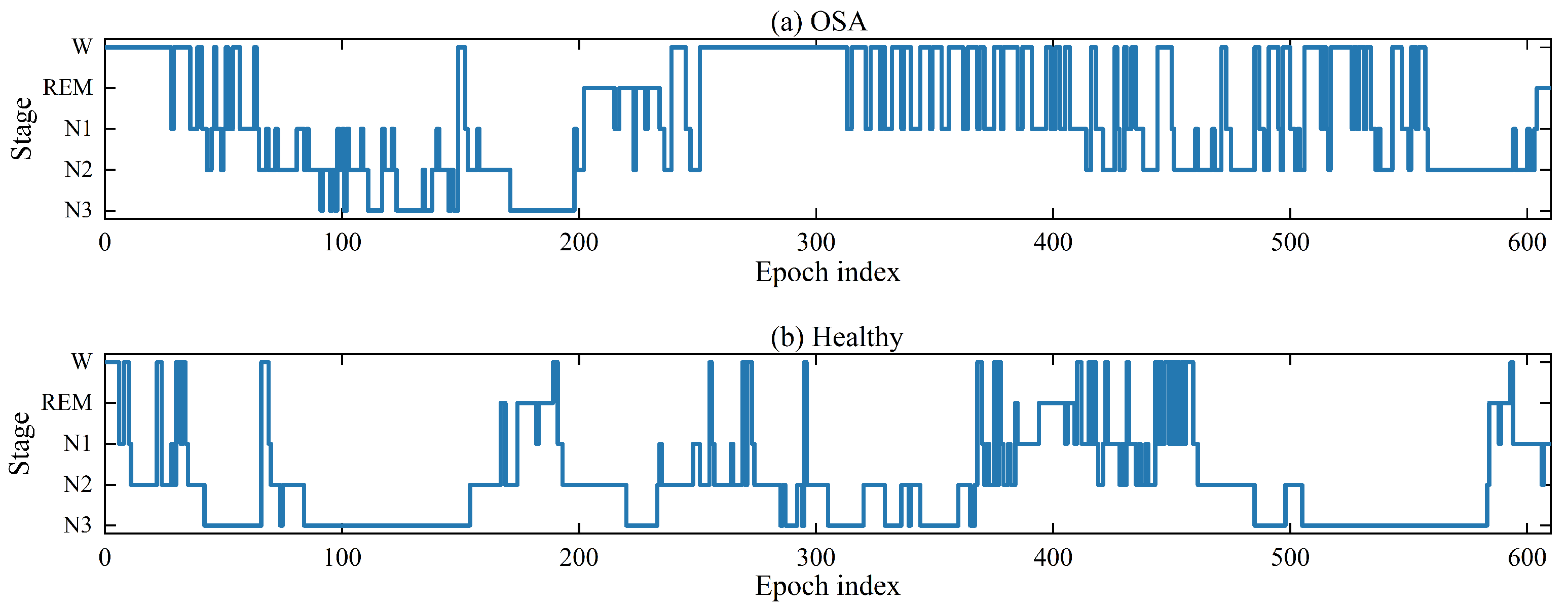Consequently, automatic sleep staging in healthy individuals has gained significant attention in recent years [9,10,11]. However, there has been limited focus on sleep staging among patients suffering from OSA. Compared to healthy individuals, OSA patients show varying degrees of oscillations in the EEG signal due to respiratory obstruction. The procedure of sleep stages in OSA patients and healthy individuals is shown in Figure 1. Both healthy and OSA people were obtained from the publicly available dataset ISRUC [12]. As shown in Figure 1, it is difficult for this OSA patient to fall into deep sleep, especially after the 300th epoch. Respiratory obstruction significantly disturbs the patient’s sleep structure and triggers dramatic EEG signal oscillations. This poses a great challenge for sleep physicians when manually labeling sleep EEG signal. They must screen for disturbed waveforms but have difficulty distinguishing sleep stages as accurately as they do with the EEG signal of normal people. It motivates the need for more robust methods.

Among the various PSG signals, EEG signals show significant changes in different sleep stages and are the most commonly used signals in sleep staging research [13,14,15,16,17,18]. The EEG signals consists mainly of the following frequency bands: delta waves, theta waves, alpha waves, sigma waves, beta waves, and gamma waves. During the REM stage, there is a noticeable increase in high-frequency waves, accompanied by the presence of theta and alpha waves. In the N1 stage, alpha wave frequency decreases and low-amplitude theta waves emerge. The prominent waveforms in the N2 stage are sleep spindles waves and K-complexes. In N3 stage, the sleep spindle wave disappears and the delta wave dominates with a significant increase in amplitude. Therefore, EEG signal based sleep staging has been widely studied [19,20].

Despite significant progress in automated sleep staging in healthy individuals [21,22], existing methods still face several challenges when applied to patients with OSA. Firstly, the EEG signals themselves have nonlinear properties. However, automated sleep staging for most OSA patients is usually performed using conventional machine learning techniques and deep learning models in Euclidean space [23,24]. Taditional methods cannot adequately capture the nonlinear interactions between EEG signal channels. Deep learning models consist of multiple layers, with each layer producing an output vector by applying a non-linear activation function to the output of the preceding layer [25]. Although deep learning-based encoders can automatically extract complex patterns and embeddings from raw EEG data, capturing both local and global dependencies. But deep learning models often require large amounts of labeled data for training, which can be a limitation in clinical settings. Secondly, the frequent oscillations of EEG signals caused by respiratory disturbances in OSA patients result in significant intra-class diversity. Since different degrees of respiratory obstruction affect EEG signal oscillations to different degrees, EEG signals can vary from one OSA patient to another, even when they are in the same sleep stage [26,27]. Thirdly, most existing methods rely heavily on static feature extraction. It fails to adequately capture the dynamic changes in EEG signals that reflect the real-time effects of respiratory events on brain activity. These dynamic changes are crucial for accurate sleep staging in OSA patients but are often neglected by current methods [28]. In addition, the cross-subject diversity of EEG signal patterns in OSA patients poses a significant challenge, as models trained from data from one patient are often difficult to generalize to other patients [29,30]. Some studies have tried to address these issues. They adopted the approach of multichannel feature extraction or nonlinear analysis. However, these methods are still inadequate. They fail to deal with the complexity of OSA-associated EEG signals effectively. In particular, they can’t capture cross-subject consistency. Also, they are unable to capture dynamic features.

Given these challenges, there is a need for a more robust sleep staging approach that can handle intra-class diversity in OSA patients while effectively leveraging the nonlinear properties of EEG signals. To address this, we propose a cross-subject classification method based on the Riemannian manifold. EEG signals from OSA patients are inherently nonlinear and highly variable. These variations result from changes in neural dynamics and physiological artifacts. Traditional Euclidean-based classifiers treat these signals as independent points in a flat space. They ignore the curved geometry created by covariance relationships among EEG channels. In contrast, Riemannian manifold analysis uses a principled approach to model these covariance structures. It preserves their intrinsic geometry and captures subtle inter-channel correlations that are crucial for accurate sleep stage discrimination. This geometric perspective forms the foundation of the proposed framework.

In recent years, Riemannian manifold-based techniques have shown promising results in EEG signal analysis [31]. Riemannian manifold-based techniques provide a geometric framework to model the inherent nonlinear structure of EEG signals, especially the covariance between multiple channels. By mapping EEG signals to the Riemannian manifold, nonlinear interactions between channels can be captured more efficiently. This is important for analyzing the complex dynamics of EEG signal in OSA patients. In addition, Riemannian methods require less data than deep learning methods and can handle intra-class diversity through domain-adaptive techniques. Deep learning encoders specialize in learning complex feature representations, while the Riemannian manifold provides a more interpretable and geometrically grounded approach for analyzing the nonlinear properties of EEG signals, especially in the context of sleep staging in OSA patients. Therefore, this paper proposes a cross-subject EEG sleep Stage Classification (EEGSSC) method based on the Riemannian manifold for OSA patients. The key contributions of this study are summarized below:

(1)

The proposed method EEGSSC is to analyze sleep EEG signal in nonlinear manifold space. Each epoch of sleep EEG signal is segmented into non-overlapping segments, mapping them on the Riemannian manifold by covariance. This transformation accounts for correlations across multiple channels and facilitates the analysis of EEG features in a nonlinear space.

(2)

In order to minimize intra-class diversity, the EEGSSC introduces a domain similarity detection module on the Riemannian manifold to address EEG diversity across different patients. This method identifies similar subjects as the source domain to assist in cross-subject sleep staging for the OSA patient.

(3)

Dynamic and static feature extraction techniques for Riemannian instances are introduced by EEGSSC. Dynamic trajectory features are extracted using the Transported Square-Root Vector Field (TSRVF), and static tangent space features are extracted by the Log-Euclidean Riemannian metric.

2. Methods

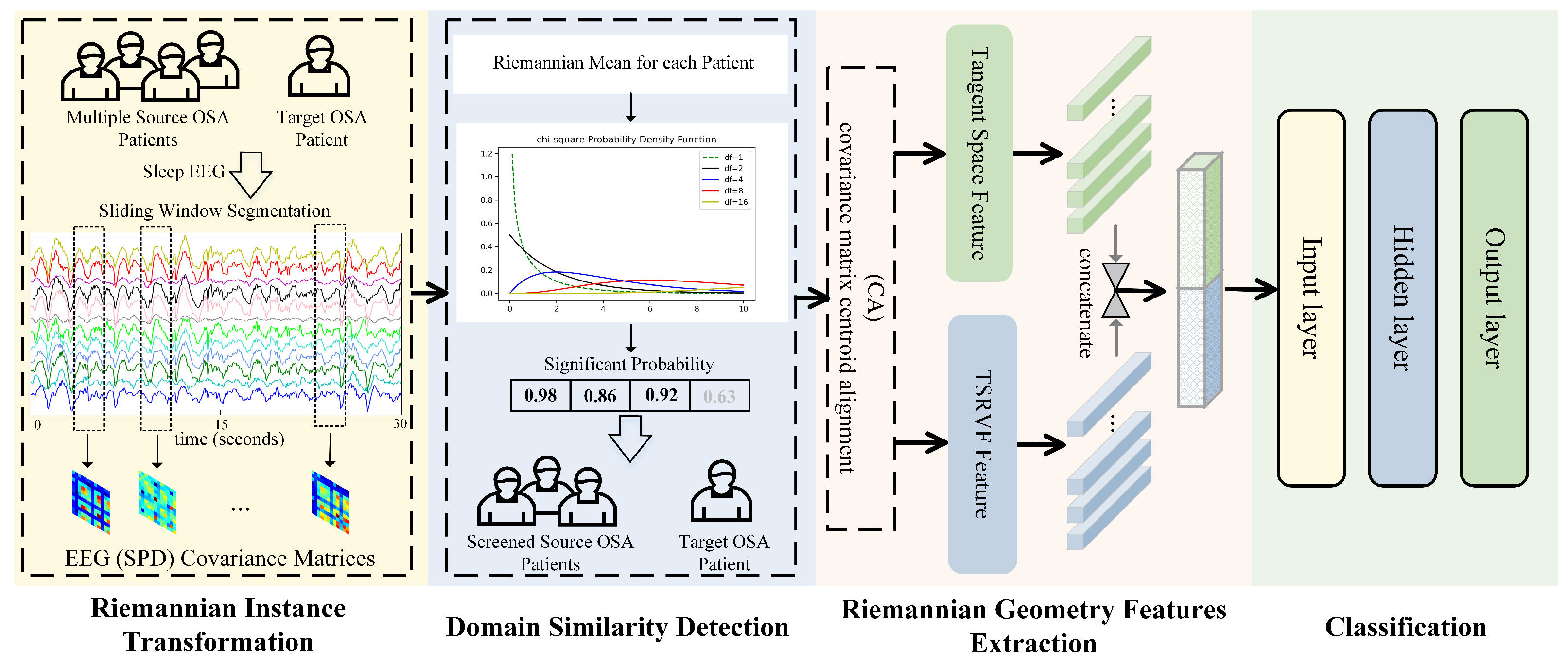
The flowchart of our automatic sleep staging method EEGSSC is shown in Figure 2. The proposed method EEGSSC consists of four main steps: (1) Riemannian instance transformation, which maps EEG signals to a nonlinear manifold space to capture the intrinsic geometric structure of the data; (2) domain similarity detection, which reduces intra-class diversity by selecting source patients similar to the target patient; (3) feature extraction, which combines both dynamic and static features using TSRVF and Log-Euclidean Riemannian metric, respectively; and (4) classification using a multi-Layer perceptron (MLP) classifier. Each step contributes to the final classification by addressing specific challenges in OSA patient EEG signal analysis, such as nonlinearity, intra-class diversity, and feature representation.

2.1. Riemannian Instance Transformation

The automated sleep staging task for OSA patients involves the intricate analysis of a 30-s epoch of EEG data to determine a sleep stage accurately. Commonly used EEG signal analysis methods are performed in Euclidean space, which cannot adequately describe the nonlinearity of EEG signals. Therefore, the nonlinear Riemannian manifold space is chosen to study the EEG signals of OSA patients. In the field of differential geometry, Riemannian manifold is a central concept. It broadens the scope of traditional Euclidean space, extending it to more general surfaces and multidimensional spaces. The symmetric positive definite (SPD) matrix manifold is a type of Riemannian manifold, which is widely used in fields such as EEG signal and image processing. In EEG signal analysis, the SPD manifold can be utilized better to capture the intrinsic geometric structure of EEG signal activity. This is important for decoding the EEG signals generated by the brain’s thinking activities. It is possible to utilize the geometric properties of the manifold for more effective feature extraction and classification by modeling the covariance matrix of the sleep EEG signal onto the SPD manifold.

The EEG signal segment with index i within the PSG data was recorded across several channels and denoted as follows:

$${\mathbf{X}}_i=\left[\begin{array}{c}\mathbf{x}\left(t\right),\dots ,\mathbf{x}\left(t+L-1\right)\end{array}\right]\in {\mathbb{R}}^{N\times L},$$

(1)

where N and L respectively signify the total count of channels and sampled points, whereas $\mathbf{x}\left(t\right)$ represents the snapshot vector, which is denoted as shown below:

$$\mathbf{x}\left(t\right)={\left[\begin{array}{c}{x}_1\left(t\right),\dots ,x_N\left(t\right)\end{array}\right]}^T\in {\mathbb{R}}^{N\times 1},$$

(2)

where T represents transpose operation. The covariance matrix pertaining to EEG signals is formally defined by the equation given as $cov=E\left(({\mathbf{X}}_i-E\left({\mathbf{X}}_i\right)){({\mathbf{X}}_i-E\left({\mathbf{X}}_i\right))}^T\right)$, the expected value, denoted as $E(·)$, serves as a quantification of the mutual dependency between channels, being the prevalent choice among second-order statistical measures. The spatial interaction between channels is fully captured within the covariance matrix. The sample covariance matrix (SCM) of ${\mathbf{X}}_i$, represented by ${\mathbf{P}}_i\in {\mathbb{R}}^{N\times N}$, encapsulates this information and can be calculated using the following formula:

$${\mathbf{P}}_i={\displaystyle \frac{1}{L-1}}{X}_i{X}_i^T.$$

(3)

The covariance matrices are symmetric and positive definite, meaning they have strictly positive eigenvalues. Let ${\mathcal{P}}_n$ represent the collection of $n\times n$ SPD matrices. These matrices lie on a differentiable Riemannian manifold, which facilitates the extraction of nonlinear geometric structures in data [32,33].

In order to extract the comprehensive features of sleep EEG signal for OSA patients on the Riemannian manifold, each 30-s sleep EEG epoch was segmented into 15 segments. Each segment is 2 s long with no overlap between segments. Let $\mathbf{X}$ denotes an epoch multi-channel EEG signal of PSG recording, then a sequence $({\mathbf{X}}_1,{\mathbf{X}}_2,\dots ,{\mathbf{X}}_{15})$ of segments is obtained by segmentation. Then, the sample covariance is computed for all segments to obtain an SPD matrices $({\mathbf{P}}_1,{\mathbf{P}}_2,\dots ,{\mathbf{P}}_{15})$ on the Riemannian manifold. A unique point on the manifold is associated with each SPD matrix, an epoch of EEG signal is permuted from a time series in Euclidean space to a sequence in a nonlinear manifold via the covariance transformation of the segments. Intuitively, this transformation projects the EEG covariance matrices into a nonlinear manifold space, allowing the model to capture intrinsic inter-channel relationships that cannot be represented in Euclidean space.

2.2. Domain Similarity Detection

Due to varying degrees of sleep-breathing obstruction in different OSA patients, their EEG signals exhibit significant intra-class diversity. Specifically, it results in large differences in EEG signal patterns over time in different patients [23,24]. To reduce this diversity, anomaly detection method based on the Hotelling theory is borrowed. Hotelling theory is a statistical abnormality detection method that is primarily used to identify outliers in multivariate data [34]. Through calculating the distance between each data point and the sample mean, the Hotelling $T^2$ statistic can be obtained, which approximates the chi-square distribution. Comparing the $T^2$ statistic to the critical value of the chi-square distribution identifies whether the data point is normal or abnormal. If the $T^2$ statistic exceeds the critical value, the data point is labeled as an outlier. This method, based on statistical principles, provides an objective way to detect anomalies in multivariate data sets.

To begin with, the OSA patient who will be sleep staged is referred to as the target patient. The other patients are referred to as source patients. Before modeling sleep staging, it is critical to select source patients that are similar to the target patient to reduce intra-class diversity. Specifically, we computed the Riemannian distance between the target patient and each source patient. Then, based on the distribution of these distances, we used Hotelling’s theory to assess the anomaly score of each source patient. In this way, we systematically selected source patients whose data are morphologically similar to the target patient’s data, thereby enhancing the training efficacy and generalizability of our model.

Let ${\mathcal{S}}^{\left(k\right)}$ represent the source patients ${\mathcal{S}}^{\left(k\right)}=\left\{{\mathbf{P}}_{\mathcal{S},i}^{\left(k\right)}\right\}$ and $\mathcal{T}$ denote the target patient $\mathcal{T}=\left\{{\mathcal{P}}_{\mathcal{T},i}\right\}$ where i refers to the index of the SCM, and $k=1,2,\dots K$ indicates the index of the source patient. The Riemannian mean for the matrices is used as descriptor for OSA patients. Specifically, the Riemannian means of ${\mathcal{S}}^{\left(k\right)}$ and $\mathcal{T}$, denoted by ${\mathbf{M}}_{\mathcal{S}}^{\left(k\right)}$ and ${\mathbf{M}}_{\mathcal{T}}$ respectively, are formally defined as:

$$M_{\mathcal{S}}^{\left(k\right)}=\underset{P\in {\mathcal{S}}^{\left(k\right)}}{arg\min }\sum _{i=1}^k{\delta }_R^2\left(P,P_{\mathcal{S},i}^{\left(k\right)}\right),$$

(4)

$$M_{\mathcal{T}}=\underset{P\in \mathcal{T}}{arg\min }\sum _{i=1}^k{\delta }_R^2\left(P,P_{\mathcal{T},i}\right).$$

(5)

The Riemannian mean differs from the arithmetic mean found in Euclidean space, as it is a geometric mean that minimizes the summation of the squared distances to all SPD matrices from the data set. Since there is no closed formula to calculate this value, optimization algorithms are required. A highly efficient iterative method for computing the Riemannian mean of SPD matrices is given in [35]. The geodesic curve between any two SPD matrices on the manifold ${\mathcal{P}}_n$ is distinct, and the Riemannian distance along this geodesic curve, based on its arc length, is defined as follows:

$${\delta }_R\left(P_1,P_2\right)={∥log\left(P_1^{-1}{P}_2\right)∥}_F={\left[\sum _{i=1}^n{log}^2{\lambda }_i\right]}^{1/2},$$

(6)

where ${\mathbf{P}}_1,{\mathbf{P}}_2\in {\mathcal{P}}_n$, ${∥·∥}_F$ denotes Frobenius paradigm for matrices, and ${\lambda }_i$ is the i-th positive eigenvalue of ${\mathbf{P}}_1^{-1}{\mathbf{P}}_2$.

We use Equation (6) to compute the Riemannian between two symmetric positive definite (SPD) matrices, which reflects the geometric difference between the matrices on the Riemannian manifold. By calculating the Riemannian distance between the target patient and source patients, we can quantify their similarity. A smaller distance indicates that the EEG signals of the two patients are more similar in their distribution on the manifold.

The procedure of domain similarity detection is as follows:

(1)

Determine the sample mean $\mu$ and the sample variance $\sigma$ for the Riemannian distances ${\delta }_R({\mathbf{M}}_{\mathcal{T}},{\mathbf{M}}_{\mathcal{S}}^{\left(k\right)})$.

(2)

Compute the domain similarity $s\left({\delta }_R\right)={({\delta }_R-\mu )}^2/{\sigma }^2$.

(3)

Assuming that $s\left({\delta }_R\right)$ follows a chi-square distribution, choose the source patient for which the Riemannian distanced ${\delta }_R$ has a significant probability of being at least parameter $\theta$ or higher.

The primary role of domain similarity detection is to reduce intra-class diversity among different OSA patients. By selecting the source patient most similar to the target patient, we ensure that the model has better generalization capabilities for cross-subject sleep staging. Specifically, domain similarity detection calculates the Riemannian distance between the target patient and source patients, selecting the most similar source patient as a reference. This reduces distributional differences between patients and improves classification accuracy. This domain similarity detection step ensures that EEG data from different patients are aligned in distributional geometry, allowing the classifier to generalize across subjects while mitigating patient-specific variability.

After reducing intra-class diversity through domain similarity detection, the next step involves extracting both dynamic and static features from the aligned data. The domain similarity detection ensures that the feature extraction process operates on a more consistent dataset, minimizing the impact of inter-patient variability.

2.3. Feature Extraction on the Manifold

The domain similarity detection reduces the differences in the data, allowing the TSRVF and Log-Euclidean Riemannian metric to more effectively capture the dynamic and static features relevant to sleep staging. For static feature extraction, all SPD matrices are projected to the tangent space using the Riemannian mean as a reference point by the Log-Euclidean Riemannian metric. Dynamic feature extraction based on TSRVF, the SPD matrices are projected into Euclidean space by capturing the dynamics of the SPD matrices along the geodesic curve. These two techniques help to efficiently extract features that maintain the inherent geometry of the data. Before feature extraction, center alignment (CA) is performed on the SCM matrix to address variations in the distribution of data edges between patients and to ensure more consistent and accurate classification. The graphical illustration of the static and dynamic feature extraction on the SPD manifold is shown in Figure 3.

2.3.1. Static Feature

The static features are derived from SPD matrices, which represent the spatial covariance structure of the EEG signals. These matrices capture the global statistical relationships between different EEG channels over a specific time window, summarizing the signal’s spatial interactions. By leveraging the properties of SPD matrices within a Riemannian geometric framework, the extracted features reflect the overall structure and stability of the EEG signals. It is widely used in the processing of EEG signal features [36].

Specifically, the computation of the centroid alignment for the source patient ${\mathbf{P}}_{\mathcal{S},i}^{\left(CA\right)}$ is formulated as follows:

$$P_{\mathcal{S},i}^{\left(CA\right)}=M_{\mathcal{T}}^{-{\displaystyle \frac{1}{2}}}{P}_{\mathcal{S},i}{M}_{\mathcal{T}}^{-{\displaystyle \frac{1}{2}}},$$

(7)

here ${\mathbf{M}}_{\mathcal{T}}$ signifies the Riemannian mean of target patient. CA reduces inter-subject variability by aligning the covariance matrices of source subjects to the Riemannian mean of the target subject. OSA patients often show large differences in EEG amplitude, oscillatory patterns, and covariance structure. As a result, the raw SPD matrices from different subjects may occupy distant regions of the manifold. This mismatch disrupts distributional consistency and complicates feature extraction and classification. Centroid alignment mitigates this issue by translating all source SPD matrices into a common reference frame. After alignment, the geometric structure becomes more consistent across subjects. This consistency yields more discriminative tangent space features and enhances cross-subject generalization.

After CA, tangent space mapping projects each SCM ${\mathbf{P}}_i$ onto the tangent space of the Riemannian manifold at ${\mathbf{P}}_{\Psi }$ as follows:

$$T_{{\mathbf{P}}_{\Psi }}\left({\mathcal{P}}_n\right)=\left\{{\mathrm{tangV}}_i=\mathrm{upper}\left({\mathbf{P}}_{\Psi }^{-{\displaystyle \frac{1}{2}}}{\mathrm{Log}}_{{\mathbf{P}}_{\Psi }}\left({\mathbf{P}}_i\right){\mathbf{P}}_{\Psi }^{-{\displaystyle \frac{1}{2}}}\right)\in {\mathbb{R}}^{n(n+1)/2}\right\}.$$

(8)

The upper$\left(·\right)$ operator is used to extract and vectorize the upper triangular portion of an SCM matrix, where the diagonal elements are given unit weights, and the off-diagonal elements are multiplied by $\sqrt{2}$ [37]. The function logm$\left(·\right)$ refers to the matrix logarithm operation, denoted as

$$Lo{g}_{P_{\Psi }}\left(P_i\right)=P_{\Psi }^{{\displaystyle \frac{1}{2}}}log\left(P_{\Psi }^{-{\displaystyle \frac{1}{2}}}{P}_i{P}_{\Psi }^{-{\displaystyle \frac{1}{2}}}\right)P_{\Psi }^{{\displaystyle \frac{1}{2}}}.$$

(9)

In addition to centroid alignment, static tangent-space features are critical for sleep stage discrimination. The Log-Euclidean Riemannian metric maps each SPD covariance matrix to a vector in a tangent space. This vector compactly represents the spatial covariance structure of EEG channels within an epoch. Such structure reflects the distribution of band-specific power across cortical regions. It also corresponds to canonical sleep phenomena, including elevated delta activity in deep sleep and the presence of spindles or K-complexes in N2. Because these tangent-space features capture stable spatial patterns, they are relatively robust to transient artifacts. They therefore provide a strong baseline representation for each epoch.

2.3.2. Dynamic Feature

The TSRVF is a mathematical framework designed to represent and analyze trajectories on the Riemannian manifold. It can represent trajectories in a way that is invariant to time-warping [38]. It also maintains geometric consistency. Time-warping invariance allows us to ignore differences in the time axis. It enables us to focus on the shape and dynamic features of trajectories. EEG data exhibit significant temporal variability, which arises from differences in time evolution, event-related potential latencies, and dynamic changes in rhythmic activity. This variability makes direct comparison and analysis challenging. The TSRVF provides a robust framework for extracting dynamic features from EEG signals. By leveraging its time-warping invariance, TSRVF can align and compare EEG signal trajectories while focusing on their shape and dynamic patterns, enabling more accurate analysis of brain activity.

Let ${\mathcal{P}}_n$ be the space of $n\times n$ matrices and ${\tilde{\mathcal{P}}}_n=\{P\mid P\in {\mathcal{P}}_n\mathrm{and}\det \left(P\right)=1\}$. The space ${\tilde{\mathcal{P}}}_n$ arises as the quotient formed by the special linear group $SL\left(n\right)=\{G\in GL(n\left)\right|det\left(P\right)=1\}$ by its closed subgroup $SO\left(n\right)$, which acts on the right equipped with an invariant metric under $SL\left(n\right)$.

Despite numerous metrics have been suggested for this space, only a few meet the criteria for Riemannian metrics. In this work, we adopt the metrics outlined in [36] because they provide a convenient expression for parallel transport. The Lie algebra of ${\tilde{\mathcal{P}}}_n$ is ${\mathcal{L}}_I\left({\tilde{\mathcal{P}}}_n\right)=\{A\mid A^T=A\mathrm{and}\mathrm{trace}\left(A\right)=0\}$, where I represents the $n\times n$ identity matrix, while the inner product on ${\mathcal{L}}_I\left({\tilde{\mathcal{P}}}_n\right)$ is denoted as $\langle A,B\rangle =\mathrm{trace}\left(A{B}^T\right)$. The tangent space at $P\in {\tilde{\mathcal{P}}}_n$ is ${\mathcal{L}}_P\left({\tilde{\mathcal{P}}}_n\right)=\{PA\mid A\in {\mathcal{L}}_I\left({\tilde{\mathcal{P}}}_n\right)\}$ and $\langle PA,PB\rangle =\mathrm{trace}\left(A{B}^T\right)$. The exponential map is given as $P\in {\tilde{\mathcal{P}}}_n$ and $V\in {\mathcal{L}}_P\left({\tilde{\mathcal{P}}}_n\right)$, ${exp}_P\left(V\right)={\left(P{e}^{2\left(P^{-1}\right)V}P\right)}^{1/2}$. For any $P_1,P_2\in {\tilde{\mathcal{P}}}_n$, the inverse exponential map is expressed as: ${exp}_{P1}\left(P_2\right)=P_1\log \left({\left(P_1^{-1}{\mathrm{P}}_2^2{P}_1^{-1}\right)}^{1/2}\right)$. Finally, for any $P_1,P_2\in {\tilde{\mathcal{P}}}_n$, the parallel transport of $V\in {\mathcal{L}}_P\left({\tilde{\mathcal{P}}}_n\right)$ from $P_1\to P_2$ is $P_2{T}_{12}^{T}B{T}_{12}$, where $B=P_1^{-1}V$,$T_{12}=P_{12}^{-1}{P}_1^{-1}{P}_2$ and $P_{12}={\left(P_1^{-1}{\mathrm{P}}_2^2{P}_1^{-1}\right)}^{1/2}$. The TSRVF pertaining to a smooth trajectory $\alpha$ on the Riemannian manifold entails the parallel transport of a proportionally velocity vector field of $\alpha$ towards a reference point $c\in {\mathcal{P}}_n$, in accordance with the following formulation:

$$h_{\alpha }\doteq {\displaystyle \frac{\dot{\alpha }{\left(t\right)}_{\alpha \left(t\right)\to c}}{\sqrt{∥\dot{\alpha }\left(t\right)∥}}}\in T_c\left({\mathcal{P}}_n\right).$$

(10)

Here, $T_c\left({\mathcal{P}}_n\right)$ represents the tangent space of at c, In this paper, the selection of the reference point corresponds to the identity matrix. The quantity $\parallel h_{\alpha }\parallel$ signifies the square-root of the instantaneous speed, whereas the ratio $h_{\alpha }/\parallel h_{\alpha }\parallel$ indicates instantaneous direction along the trajectory. The TSRVF representation based feature for source patients and target patient is given by

$${\mathrm{tsrvfV}}_{\mathcal{S},i}=\mathrm{upper}\left(h_{\alpha (\mathcal{S},i)}\right),{\mathrm{tsrvfV}}_{\mathcal{T},i}=\mathrm{upper}\left(h_{\alpha (\mathcal{T},i)}\right),$$

(11)

where $h_{\alpha }\left(\mathcal{S},i\right)$ and $h_{\alpha }\left(T,i\right)$ denote the TSRVF in the source and target patients respectively.

The TSRVF representation captures the dynamic evolution of SPD matrices within each 30-s epoch by encoding the geodesic velocity field of the covariance-matrix trajectory. Static covariance features do not retain this dynamic information. The TSRVF preserves temporal changes such as stage transitions, spindle activity, and micro-arousal-related oscillations. These dynamics are essential for distinguishing sleep stage. The TSRVF is also invariant to temporal misalignment caused by time-warping. This property allows trajectories with different lengths or rhythmic patterns to be compared consistently. As a result, the representation becomes more robust to patient-specific variability in EEG temporal dynamics.

2.3.3. Feature Fusion

The static features (tangV) and dynamic features (tsrvfV) are fused through direct concatenation of all feature vectors. Specifically, for each 30-s EEG epoch, we concatenate all 15 static feature vectors ($\mathrm{tangV}\in {\mathbb{R}}^{N(N+1)/2}$) and all 15 dynamic feature vectors ($\mathrm{tsrvfV}\in {\mathbb{R}}^{N(N+1)/2}$) extracted from the sub-segments, forming the final feature representation ($\mathrm{f}\in {\mathbb{R}}^{15\times N(N+1)}$), which serves as input to the classifier.

2.4. Sleep Staging

The proposed EEGSSC method consists of four main steps: Riemannian instance transformation, domain similarity detection, feature extraction on the SPD manifold, and classification. In this subsection, we elaborate on the final step, sleep staging, which involves the classification of sleep stages using a MLP classifier.

After extracting both static and dynamic features from the Riemannian manifold, these features are concatenated to input the MLP classifier. The MLP architecture consists of three layers. The Adam optimizer is employed to train the model efficiently. To prevent overfitting, dropout layers are added between the fully connected layers. The MLP classifier outputs the predicted sleep stage for each 30-s epoch. The final classification is based on the softmax activation function, which provides a probability distribution over the five sleep stages (W, N1, N2, N3, and REM). The complete workflow of the EEGSSC method is summarized in Algorithm 1, which outlines the steps from EEG signal processing to sleep stage classification.

Algorithm 1 The proposed EEGSSC method.

Input: k source patients training data ${\mathcal{S}}^{\left(k\right)}$ and target patient data $\mathcal{T}$ in ${\mathcal{P}}_n$.   Output: Predicted classes $y_{\mathrm{test}}$ of $\mathcal{T}$. 1: /* Source patient select */ 2: Calculate Riemannian mean for each source patient ${\mathbf{M}}_S^{\left(k\right)}$ and target patient ${\mathbf{M}}_T$ using (4) and (5). 3: Determine the mean ($\mu$) and variance ($\sigma$) of the Riemannian distances ${\delta }_R({\mathbf{M}}_T,{\mathbf{M}}_S^{\left(k\right)})$. 4: Compute the domain similarity $s\left({\delta }_R\right)={({\delta }_R-\mu )}^2/{\sigma }^2$. 5: Choose the $k^{\prime }$ source patient whose significant probability of $\theta$ or greater. 6: /* Model training */ 7: Align SCMs of the selected source patients ${\mathbf{P}}_{S,i}^{\left(CA\right)}$ using (7). 8: Extract tangent feature for the selected source patients ${\tan \mathrm{gV}}_{S,i}$ using (8). 9: Extract trajectory feature for the selected source patients ${\mathrm{tsrvfV}}_{S,i}$ using (10) and (11). 10: Training MLP classifier on the data representation. 11: /* Testing phase */ 12: Extract tangent feature for target patient ${\tan \mathrm{gV}}_T$ using (8). 13: Extract trajectory feature for target patient ${\mathrm{tsrvfV}}_T$ using (10) and (11). 14: $y_{\mathrm{test}}\leftarrow$ MLP using the feature vector. 15: return Predicted classes $y_{\mathrm{test}}$.

3. Experiment

3.1. Dataset

We validated the EEGSSC method on the ISRUC [12] and Dreem [39] datasets, both of which contain PSG recordings from sleep apnea patients. The following is a detailed description of the datasets.

The ISRUC dataset contains three subsets, subgroup-$\mathrm{II}$ is PSG data in subjects suffering from sleep apnea. It contains PSG data from 8 patients for two nights (session 1 and session 2). The dataset includes six EEG signal channels: F3-A2, C3-A2, O1-A2, F4-A1, C4-A1, and O2-A1, sampled at 200 Hz. Preprocessing involved applying a 50-Hz notch filter and a 0.3-Hz to 35-Hz Butterworth bandpass filter. Sleep stages for each night were independently assessed by two specialists following the AASM criteria.

The Dreem dataset comprises the Dreem Open Dataset-Obstructive (DOD-O), containing full-night PSG recordings from 56 patients diagnosed with OSA. The EEG was recorded using eight channels: C3-M2, C4-M1, F3-F4, F3-M2, F4-O2, F3-O1, O1-M2, and O2-M1, with a sampling frequency of 250 Hz. A bandpass filter set between 0.4 Hz and 18 Hz was applied during pre-processing. All PSG recordings were annotated according to AASM guidelines by five different sleep experts, with each segment lasting 30 s.

3.2. Methods of Comparison

We performed comparison experiments on ISRUC and DOD-O datasets to validate our approach. Specifically, we used five different comparison methods. They are described in detail below:

SVM [22]: involves a classification model for sleep stages based on seven EEG signal sub-bands (0.5–2 Hz, 2–6 Hz, 4–8 Hz, 8–13 Hz, 12–14 Hz, 12–30 Hz, and 30–49.5 Hz). This model utilizes four time-domain features and one from the time-frequency domain, specifically Normalized Sub-band Power, Inter-quartile Range, Mean Absolute Deviation, Movement, and features derived from the Fourier Synchrosqueezed Transform. The Support Vector Machine (SVM) classifier is then assessed using these datasets.

Ensemble SVM [40]: employs multivariate phase space reconstruction to create covariance matrices on the Riemannian manifold. These matrices are subsequently projected to the tangent space of the Riemannian geometric mean. These tangent space feature vectors were categorized into different sleep stages using an ensemble classifier.

Ensemble DT [36]: utilizes covariance matrices derived from multiple channels to analyze inter-dependencies. Tangent vectors are then computed using Riemannian geometry, with these features fed into an ensemble classifier that employs bagging techniques.

MDM [41]: employs spatial covariance matrix representation for sleep EEG data, and is evaluated by Riemannian Manifold Distance to Mean (MDM) classification algorithms.

RKNN [41]: employs spatial covariance matrix representation for sleep EEG data, and is evaluated by Riemannian K-Nearest-Neighbours (RKNN) classifier using Riemannian distance.

NeuroNet [42]: includes a multiscale 1D ResNet-based frame network for feature extraction, and a Mamba-based temporal context module to capture relationships between EEG epochs.

Sleepyco [43]: uses a feature pyramid and supervised contrastive learning to classify single-channel EEG signals. It incorporates a feature pyramid to capture multi-scale temporal and frequency information, and uses supervised contrastive learning to enhance class discrimination.

XSleepNet [44]: consists of two network streams: one for raw signals using a fully convolutional neural network and another for time-frequency images using an attention-based recurrent neural network.

3.3. Performance Metrics

In this paper, six evaluation metrics were used to assess the performance of sleep staging models. Precision (Pre), Recall (Rec), and per-class F1 score (F1) were applied to quantify the classification accuracy for individual sleep stages. To comprehensively evaluate the overall effectiveness across all categories, Macro-averaged F1 score (MF1), Accuracy (Acc), and Cohen’s kappa ($\kappa$) were utilized. The formal definitions of these metrics are defined as follows:

$$\mathrm{Pre}={\displaystyle \frac{TP}{TP+FP}},$$

(12)

$$\mathrm{Rec}={\displaystyle \frac{TP}{TP+FN}},$$

(13)

$$F1={\displaystyle \frac{2\left(Pre\times Rec\right)}{Pre+Rec}},$$

(14)

$$\mathrm{MF}1={\displaystyle \frac{1}{C}}\sum _{i=1}^{C}F{1}_i,$$

(15)

$$\mathrm{A}cc={\displaystyle \frac{TP+TN}{TP+FP+FN+TN}},$$

(16)

$$\kappa ={\displaystyle \frac{p_o-p_e}{1-p_e}}.$$

(17)

True Positives (TP) represent the count of instances where the actual sleep stage was accurately classified. False Positives (FP) refer to cases where a different sleep stage was incorrectly identified as the current stage. Conversely, False Negatives (FN) occur when the actual sleep stage is misclassified as another stage. True Negatives (TN) denote instances where other stages were correctly classified as not being the current sleep stage. The number of sleep stage categories is represented by C, while po indicates the observed agreement between raters, pe denotes the expected probability of agreement based on random chance.

3.4. Experimental Setup

In this study, the k-fold cross-validation method was used for sleep stage classification. For the ISRCU dataset, a k value of 16 was used, which is equal to leaving one subject for cross-validation. In each iteration, 15 subjects were utilized for model training and the remaining subjects were used as the test set. This process was iterated until all 16 subjects were accurately assigned to the test set once, thus ensuring a full evaluation of the entire population. In contrast, we used 3-fold cross-validation for the Dreem dataset due to its much larger sample size and the time-consuming nature of k-fold cross-validation. In the experiment, the parameter $\theta$ was assigned a value of 0.75. The MLP architecture consists of three layers, where the amount of neurons is set to 200, 100, and 50 in each layer, respectively. The Adam optimizer was employed with a learning rate of 0.0001 to ensure efficient training. The batch size was fixed at 64 and the number of model training epochs set to 900. All experiments were performed using a machine equipped with an Intel Xeon W-2255 @ 3.70-GHz CPU and 64-GB RAM (Dell Inc., Round Rock, TX, USA).

4. Results

4.1. Effect of Domain Similarity Detection

The confusion matrices for the model both with and without domain similarity detection on ISRUC subgroup-$\mathrm{II}$ and DOD-O dataset are provided in Figure 4 and Figure 5. The confusion matrix is derived by aggregating the test set results across all folds, where the predicted labels and true labels from each fold are collected and compiled together to provide a comprehensive overview of the model’s performance. Rows correspond to the true sleep stages, while columns indicate the predicted stages. As illustrated in Figure 4a, the value 121 at the intersection of the first row and second column indicates that 121 epochs of the W stage were incorrectly classified as N1. The right side of the subfigure displays the performance metrics for all five sleep stages, computed from the confusion matrix.

As shown in Figure 4 and Figure 5, without domain similarity detection, diagonal values in the confusion matrix decrease. This illustrates the effectiveness of the proposed module. Only a small increase in the REM stage was observed on the ISRUC dataset. When domain similarity detection is not used, the ACC on ISRUC and DOD-O datasets were 69.87% and 72.46%, $\kappa$ were 60.60% and 58.52%, and MF1 were 65.01% and 60.13%. When after using domain similarity detection, the ACC on the ISRUC and DOD-O datasets were 72.13% and 74.24%, $\kappa$ were 63.69% and 61.22%, and MF1 were 67.40% and 62.19%.

As shown in

Table 1. The per-class metrics based on domain similarity detection on ISRUC subgroup-$\mathrm{II}$ dataset. Domain similarity detection (a), without domain similarity detection (b).

Per-Class Metrics (%)
(a)				(b)
	Pre	Rec	F1		Pre	Rec	F1
W	70.69	79.10	74.66	W	69.80	67.61	68.69
N1	33.26	26.57	29.54	N1	31.84	24.35	27.60
N2	72.58	72.66	72.62	N2	69.00	73.00	70.94
N3	83.98	95.32	84.65	N3	82.93	82.89	82.91
REM	76.83	74.25	75.52	REM	72.73	77.31	74.95

and

Table 2. The per-class metrics based on domain similarity detection on DOD-O dataset. Domain similarity detection (a), without domain similarity detection (b).

Per-Class Metrics (%)
(a)				(b)
	Pre	Rec	F1		Pre	Rec	F1
W	72.52	71.18	71.84	W	69.50	67.53	68.50
N1	27.27	11.42	16.10	N1	26.89	9.80	14.37
N2	77.74	84.20	80.84	N2	76.43	82.88	79.53
N3	73.45	65.75	69.39	N3	70.11	64.28	67.07
REM	71.63	73.90	72.75	REM	69.71	72.77	71.20

, N1 consistently has the lowest F1 score among all stages, with or without the domain similarity detection module. The confusion matrix reveals that N1 is frequently misclassified as N2, REM, or W. Misclassifications mostly occur as N1 being mistaken for N2, while the reverse is less common. This is due to N1’s transitional and ambiguous nature, lacking distinct landmarks. N1 brain waves are dominated by low-amplitude mixed frequencies (theta waves at 4–7 Hz), which overlap with alpha waves during wakefulness (8–13 Hz) and are hard to distinguish, especially in early sleep stages. This overlap causes N1 to be misdiagnosed as REM or N2. In OSA patients, frequent microarousals from respiratory events interrupt N1, segmenting it into Wake or N2. Respiratory effort, hypoxia, and motor artifacts also obscure N1’s theta waves, leading to misclassification. Additionally, increased sleep pressure in OSA patients accelerates entry into N2/N3, reducing N1 duration. These factors make N1 challenging for our model.

4.2. Result of the Comparative Methods

We compared our proposed model with several models from other studies, using the publicly available ISRUC and DOD-O datasets and applying the same cross-validation (k-fold or leave-one-out) applied consistently. All results are derived after summarizing all test folds. As shown in Figure 6, the classification accuracy of our method is substantially ahead of MDM and RKNN, and slightly higher than the other methods, at 72.13% on the ISRUC dataset and 74.24% on the DOD-O dataset. The overall results and F1 scores for each class are detailed in

Table 3. Comparison with other methods on ISRUC subgroup-$\mathrm{II}$ dataset.

Method	Per-Class F1 (%)					Overall Metrics (%)
	W	N1	N2	N3	REM	Acc	MF1	Kappa
SVM	60.96	14.19	66.21	69.04	70.67	63.28	56.21	50.69
Ensemble SVM	77.58	11.21	72.56	79.94	71.62	71.11	62.58	61.33
Ensemble DT	81.91	22.49	72.56	77.34	59.53	69.59	62.77	59.71
MDM	24.75	21.22	23.46	48.63	25.34	31.21	28.68	13.50
RKNN	47.83	19.63	52.42	49.39	41.19	45.78	42.09	29.63
NeruONet	69.92	24.47	70.23	81.61	68.99	68.25	63.04	58.60
Sleepyco	70.67	25.71	70.58	82.30	71.84	69.21	64.22	59.87
XSleepNet	69.89	24.64	70.20	81.94	69.80	68.46	63.29	58.85
Ours	74.66	29.54	72.62	84.65	75.52	72.13	67.40	63.69

and

Table 4. Comparison with other methods on DOD-O dataset.

Method	Per-Class F1 (%)					Overall Metrics (%)
	W	N1	N2	N3	REM	Acc	MF1	Kappa
SVM	64.13	5.89	78.09	61.13	61.92	68.95	54.23	52.31
Ensemble SVM	74.35	6.37	81.07	64.81	65.65	73.29	58.45	59.32
Ensemble DT	78.43	11.49	80.58	66.44	65.43	73.62	60.47	60.41
MDM	25.94	12.07	53.27	49.77	45.17	43.46	37.24	25.47
RKNN	58.06	12.75	70.14	55.80	41.68	58.82	47.69	39.31
NeruONet	69.72	13.98	79.31	66.97	70.76	72.34	60.25	58.56
Sleepyco	69.83	14.47	79.36	67.21	70.85	72.45	60.34	58.72
XSleepNet	69.75	14.17	79.33	67.08	70.79	72.38	60.22	58.62
Ours	71.84	16.10	80.84	69.39	72.75	74.24	62.19	61.22

. Our method outperformed the others in overall metrics, with MF1 and kappa scores of 67.40% and 63.69% on the ISRUC dataset, and 62.19% and 61.22% on the DOD-O dataset. However, the F1 score of our method in the W stage on ISRUC (74.66%) was lower than Ensemble DT (81.91%), and on the DOD-O dataset, our F1 scores in the W stage (71.84%) and N2 stage (80.84%) were lower than Ensemble SVM (78.43%) and Ensemble DT (81.07%), respectively. As shown in Table 1, the F1 scores for all methods in the N1 stage are below 30%. This is primarily due to the transitional and ambiguous nature of the N1 stage, which lacks distinct and unique features.

4.3. Visualization

In order to illustrate the necessity of data alignment, the t-SNE [45] technique is performed to visualize how CA operations reduce individual distributional variations. The t-SNE technique visualizes high-dimensional data by giving each data point a location in 2D or 3D space. We calculate the covariance matrix of the raw EEG data and the covariance matrix after CA operation, and then visualize the SPD matrix data using the t-SNE technique to better observe cross-subject effects on sleep staging. In our case, each SPD matrix is a point in 2D space. The data from the ISRUC dataset for 8 patients is shown in Figure 7. It can be seen that Figure 7a shows the raw data and Figure 7b shows the data after CA operation, both using colors to identify the patients. We can observe that there is a clear separation between each patient in the raw data. Based on this situation, we considered it crucial to select source patients that are similar to the target patient. Therefore, training the classifier on the raw data may not result in good performance. After a CA operation, the data of different patients overlap each other. This means that the differences between different patients are reduced.

5. Discussion

The proposed method includes detailed mathematical derivations. However, its core idea is simple: the Riemannian representation aligns the geometry of EEG feature spaces across subjects. It also captures temporal evolution through manifold trajectories. Modeling both spatial and temporal dynamics improves interpretability and robustness in sleep stage classification.

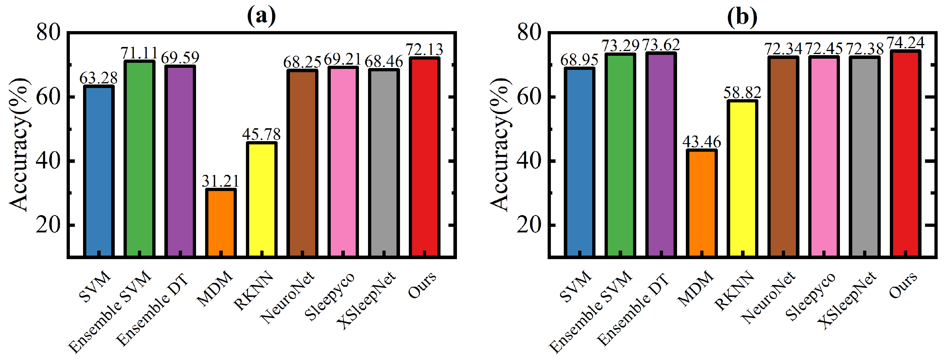
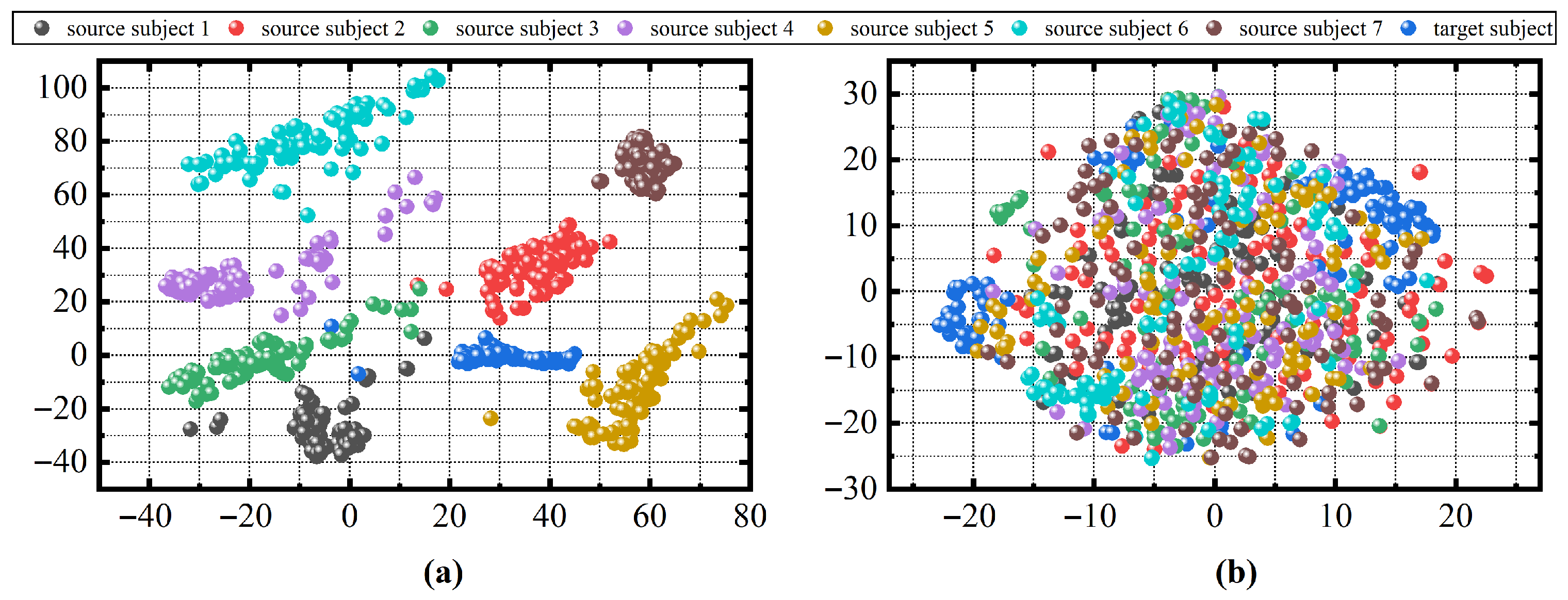
The effectiveness of the proposed domain similarity detection module is evident from the ablation experiments. By comparing our method with other existing approaches, we demonstrate that our proposed method generally outperforms the others, primarily due to the comprehensive feature extraction on the Riemannian manifold, which includes both static and dynamic features. These features effectively capture the intrinsic geometric structure of EEG signals, thereby enhancing the accuracy and robustness of sleep stage classification.

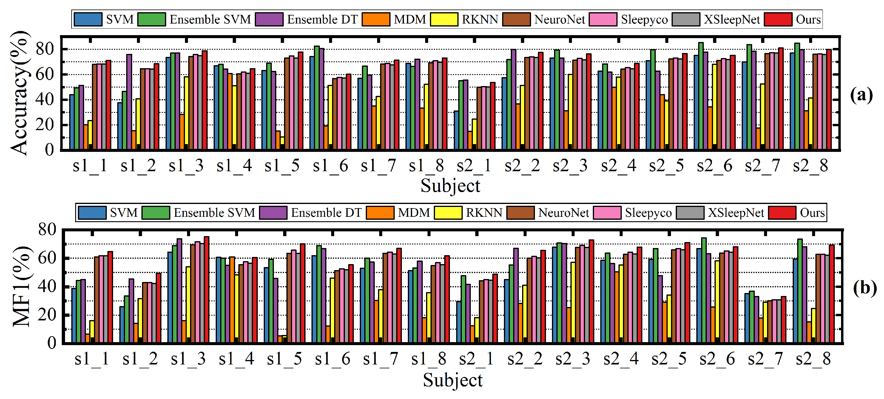
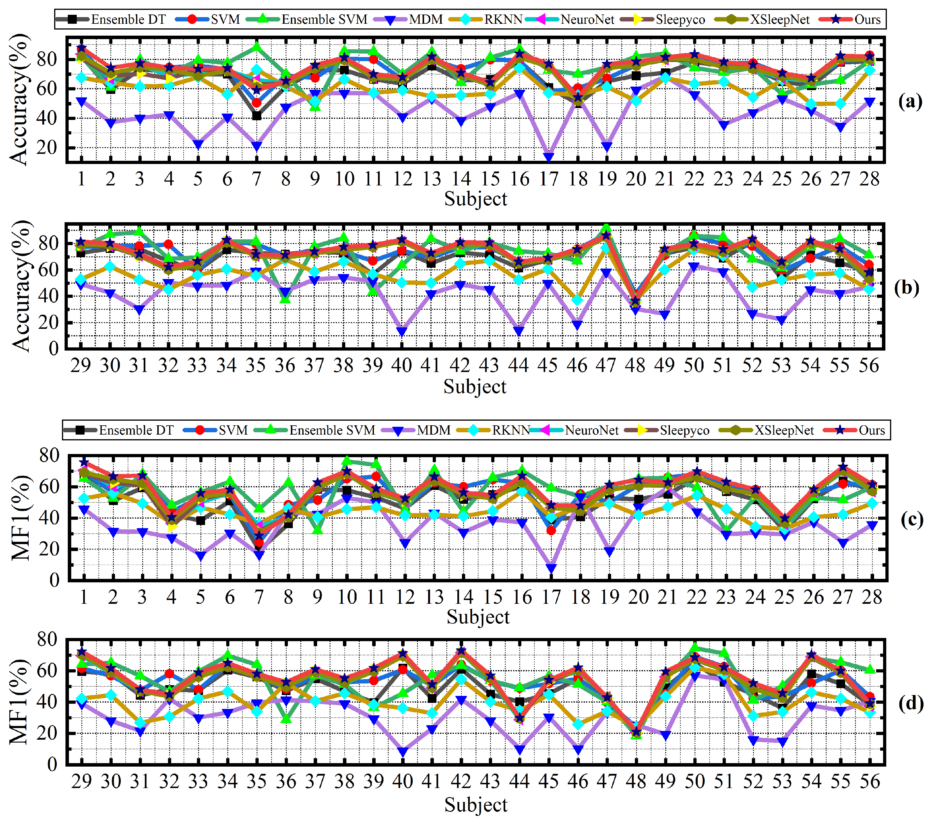
Despite the promising results achieved, our proposed method still has several limitations. Specifically, our method is designed for cross-subject sleep staging, which means that in some patients, the accuracy may be lower than that of certain other methods. Specifically, as shown in Figure 8, the Ensemble SVM method significantly outperforms our method in classifying patients s1_6 and s2_6. Similarly, Figure 9 illustrates that Ensemble SVM also achieves better classification results than our method in subjects numbered 6, 7, 8, 10, and others. The Ensemble SVM employs phase space reconstruction for multichannel EEG signals. This technique reconstructs single-channel time series into multidimensional phase space trajectories, thereby enhancing the feature representation capability.

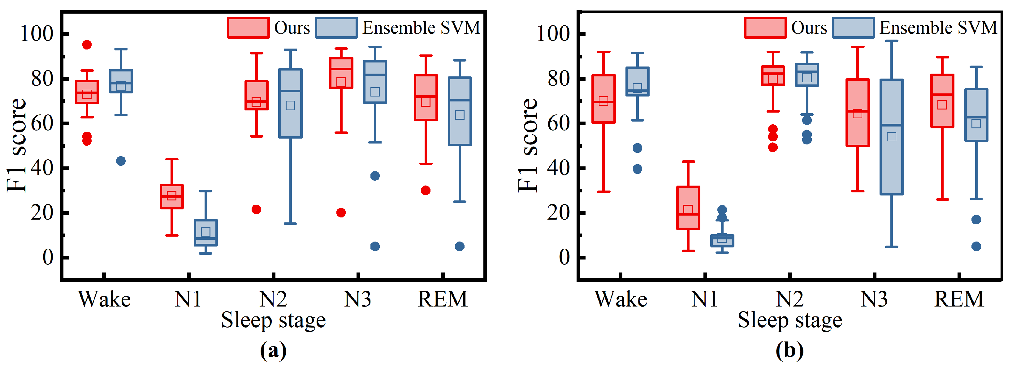
To further investigate the differences between our method and Ensemble SVM, we have statistically analyzed the F1 scores of both methods for each sleep stage across all patients, as shown in Figure 10. For the ISRUC dataset, our method demonstrates better robustness in the N2 and REM sleep stages, as indicated by the higher median values and smaller interquartile ranges (IQRs) in the box plots. However, in the Wake stage, the Ensemble SVM method shows superior robustness, with higher medians and narrower IQRs in the box plots, suggesting more stable performance in these stages. For the DOD-O dataset, Ensemble SVM also exhibits better robustness in the Wake stage, with higher medians and narrower IQRs in the box plots. Although our method has a slightly higher median in the N2 and REM stages, indicating a marginal performance advantage, the larger IQRs suggest slightly inferior robustness compared to Ensemble SVM. In the N3 stage, both methods show comparable robustness, with similar medians and IQRs in the box plots indicating similar levels of performance stability.

A novel cross-subject EEG sleep staging method (EEGSSC) was introduced in this study. The method is based on the Riemannian manifold technique and is specifically designed for patients with OSA. It effectively addresses the challenges associated with the nonlinear characteristics of EEG signals and intra-class variations due to respiratory disruptions. Through transforming EEG signals into SPD matrices, employing domain similarity detection, and extracting both dynamic and static features, EEGSSC achieves superior performance in sleep stage classification compared to existing methods. Experimental validation on the ISRUC and Dreem datasets demonstrates their high accuracy and robustness, with an overall accuracy of 72.13% and MF1 score of 67.40% on the ISRUC dataset, and an accuracy of 74.24% and an MF1 score of 62.19% on the Dreem dataset. These results highlight the potential of EEGSSC for clinical applications, particularly in the diagnosis and monitoring of OSA patients.

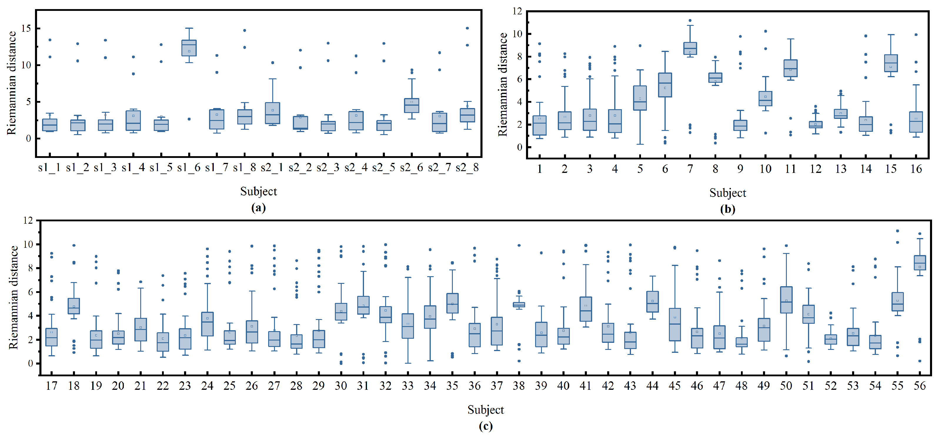
To further investigate why our method performs poorly on these patients, we first obtained the representation of each patient in the manifold using Equations (4) and (5). We then calculated the Riemannian distance between each patient and the others by Equation (6). As shown in the box plot in Figure 11, patients with more compact distances to other patients tend to have better classification results, such as patient s1_1 in the ISRUC dataset and patients 1 and 40 in the DOD-O dataset. In contrast, those with more dispersed distances have poorer classification outcomes, like patients s1_6 and s2_6 in the ISRUC dataset and patients 6, 7, 8, 10, etc., in the DOD-O dataset. This indicates that OSA patients with greater distances from each other exhibit larger distribution differences on the manifold, which poses greater challenges for sleep staging. The cause of these differences may be attributed to varying degrees of respiratory obstruction during sleep, which in turn have different impacts on sleep EEG signal and ultimately lead to distribution differences on the manifold.

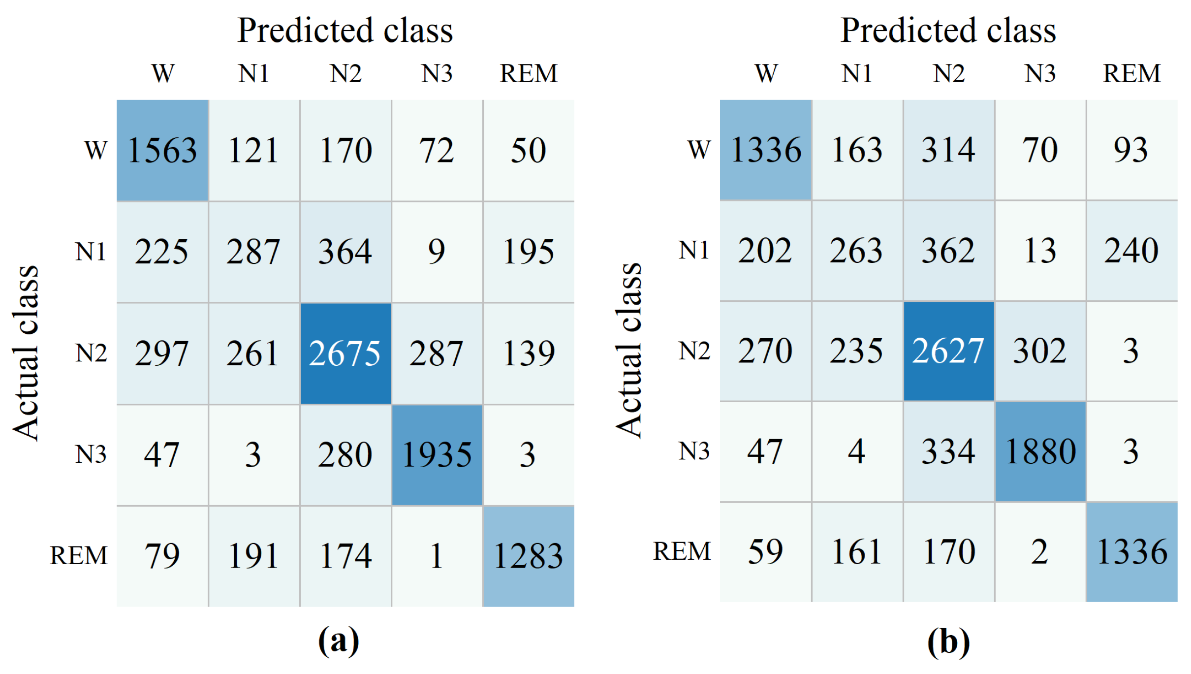
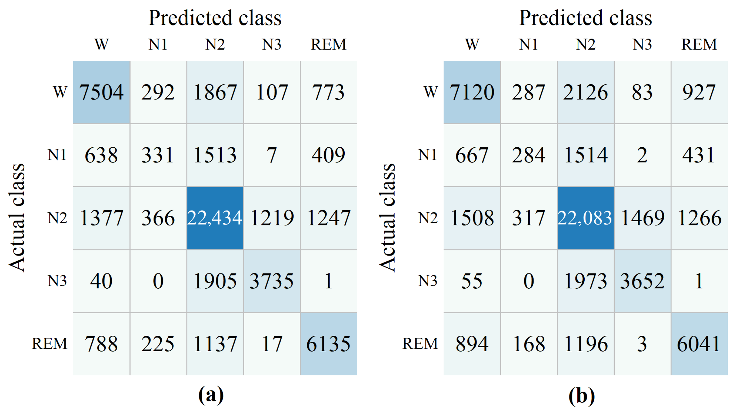
Although the proposed method performs well overall, the N1 stage remains difficult to classify. The misclassification of N1 arises from intrinsic limitations in both static SPD features and TSRVF-based dynamic representations. Static covariance matrices encode only stable inter-channel dependencies. They characterize well-defined stages such as N2 or N3. They do not sufficiently capture N1. Its spatial coupling is weak and rapidly varying. It often resembles attenuated wakefulness or early N2 patterns. Consequently, tangent-space projections derived from these SPD matrices fail to delineate clear stage boundaries. Dynamic TSRVF features face similar constraints. They assume coherent within-stage temporal evolution. This assumption breaks down for N1 in OSA patients. N1 is dominated by irregular micro-arousals and apnea-related fluctuations. These events yield short, noisy, and highly overlapping manifold trajectories, particularly around W–N2 transitions. These factors jointly reduce the discriminability of N1. They underscore the need for more sensitive temporal–spectral markers or adaptive multimodal cues. Such approaches may better capture the subtle and unstable characteristics of this stage.

In the present study, we used only conventional band-pass and notch filters for EEG preprocessing. These filters primarily remove baseline drift and power-line interference. They are widely adopted in sleep EEG research. However, such a minimal preprocessing pipeline may be insufficient for suppressing ocular, muscular, and motion artifacts. This limitation becomes pronounced when artifacts are non-stationary or overlap with task-relevant frequency bands. Residual artifacts can distort the covariance structure of EEG signals. They can also affect the construction of SPD matrices on the Riemannian manifold. Consequently, they may influence the performance of the proposed method. Enhanced EEG denoising could employ Independent Component Analysis (ICA) for artifact removal. ICA can reduce contamination from eye movements, muscle activity, and other non-neural sources. Deep learning–based denoising, such as autoencoder models, provides an alternative. Such methods may offer more robust artifact suppression.

6. Conclusions

A novel cross-subject EEG sleep staging method (EEGSSC) was introduced in this study. The process is based on the Riemannian manifold technique and is specifically designed for patients with OSA. It effectively addresses the challenges associated with the nonlinear characteristics of EEG signals and intra-class diversity due to respiratory disruptions. Through transforming EEG signals into SPD matrices, employing domain similarity detection, and extracting both dynamic and static features, EEGSSC achieves superior performance in sleep stage classification compared to existing methods. Experimental validation on the ISRUC and Dreem datasets demonstrates their high accuracy and robustness, with an overall accuracy of 72.13%, an MF1 score of 67.40% on the ISRUC dataset, and an accuracy of 74.24% and an MF1 score of 62.19% on the DOD-O dataset. These results highlight the potential of EEGSSC for clinical applications, particularly in the diagnosis and monitoring of OSA patients.

7. Future Work

Although the proposed EEGSSC framework demonstrates promising performance on both ISRUC and Dreem datasets, several important directions remain for future investigation. In future work, we will address the current multi-step structure of the method, which limits its practicality in real-time settings. We plan to develop an end-to-end multimodal Riemannian deep network that integrates EEG, EOG, and EMG signals. This approach may reduce confusion among N1, W, and N2 stages and, at the same time, simplify the processing pipeline to enable real-time sleep staging.

Additionally, scaling to larger and more heterogeneous datasets will be important for improving generalization. Cross-dataset adaptation, semi-supervised learning, and adaptive domain alignment strategies may help reduce dataset-specific bias and enhance reliability across different clinical centers. These extensions will further promote the applicability of EEGSSC in routine diagnosis and longitudinal monitoring of OSA patients.