Abstract
To enhance the survivability of unmanned aerial vehicles (UAVs) in complex electromagnetic environments, a model is presented to assess the complex electromagnetic interference (EMI) effects on UAV data links. Based on the mechanism of electromagnetic interference, three key parameters are introduced: the loss-of-lock threshold At, the effect–time ratio D, and the effect index τ. An assessment model is then developed using these parameters. By classifying interference into sinusoidal-type and noise-type, the model is capable of predicting the interference effects of complex interference scenarios comprising in-band single-tone, partial-band noise, and out-of-band interferences that generate in-band third-order intermodulation components. Measurements of At and D from single-source EMI effect tests, along with validation from three-source and four-source EMI effect tests, confirm the model’s efficacy. Results indicate that the At is inversely proportional to the D and correlates with the bit error rate. The maximum error between the experimental and theoretical values of τ is 0.709 dB, demonstrating the validity and applicability of the model. Finally, a four-level EMI effect assessment method was proposed. The assessment method could provide theoretical support for anti-interference decision-making systems and enhance the UAVs’ anti-interference capability in complex electromagnetic environments.
1. Introduction
Unmanned aerial vehicles (UAVs) are widely used in battlefields due to their advantages, such as low cost, operational flexibility, and reduced personnel casualties [1,2,3]. Data links are critical interaction systems between UAVs and the ground control station (GCS). They must operate securely and stably to ensure the successful execution of important tasks [4,5]. However, UAVs and GCS have a long communication distance. This makes data links highly vulnerable to electromagnetic interference (EMI) in battlefield environments. With the increasing informatization of weapon systems, the electromagnetic environment in modern battlefields has become increasingly complex. The UAVs now face not only intentional EMI from enemies’ interference machines but also EMI from high-power spectrum-dependent equipment [6,7]. These interferences include both in-band and out-of-band interferences. For UAVs with robust shielding capabilities, interferences mainly couple with the receivers of UAVs through the antennas, leading to the UAVs’ communication breakdown. Therefore, it is important to assess the complex EMI effects on data links so that UAVs can avoid EMI risk region and enhance their survivability in battlefield environments.
Many researchers have investigated the impact of various interferences on UAV data links via simulation and experimental methods. Lan et al. employed an UAV to enable integrated communication and over-the-air computation, and the anti-interference performance was obtained by simulation [8]. Tayebi et al. presented a bit error rate model for direct sequence spread spectrum systems and evaluated its anti-jamming performance through MATLAB simulations [9]. Luo et al. proposed a cognitive MIMO-based multidomain method to effectively suppress narrowband interference in UAV links [10]. Pan et al. used the radiated susceptibility test method to study the impact of electromagnetic pulse on the data link [11]. Mao et al. studied the high-power microwave (HPM) impact on the UAV through the radiated susceptibility test and simulation methods [12]. Zhang et al. integrated irradiation tests with co-simulation, identified the cable-coupled pathway of HPM damage in UAVs, and proposed effective countermeasures [13]. These studies focused on the mechanism and impact of different types of interference.
To evaluate the effects of interferences, many researchers have used mathematical modeling and deep-learning algorithms to assess interference effects. Cai et al. proposed a novel electromagnetic compatibility evaluation method for receivers that quantitatively correlates pulsed interference parameters with the bit error rate (BER), and validated it using radiated susceptibility tests [14]. Xu et al. used the multi-task convolutional neural network with multi-input (MIMT-CNN) to evaluate the effects of in-band single-source single-tone and partial-band noise interferences [15]. The above studies could be used to predict single-source interference effects. Li et al. developed mathematical models to predict the effects of multi-source in-band single-tone interferences [16], which are based on loss-of-lock thresholds of the interferences. Zhang et al. combined a mathematical model and GA-XGBoost to predict loss-of-lock thresholds and assess the effects of in-band multi-source interferences [17]. These studies could assess in-band interference effects. In battlefields, out-of-band interferences are as prevalent as in-band interferences. They can generate third-order intermodulation (IM3) interferences, which pose significant threats to data links [18]. Zhang et al. established an IM3 effect prediction model to predict the effects of multi-source out-of-band interferences [19].
Based on the above studies, this paper proposes a model to assess complex multi-source EMI effects, including in-band single-tone, in-band partial-band noise, and out-of-band single-tone interferences that can generate in-band IM3 interferences, on UAV data links. Initially, the interference mechanisms are analyzed, and four critical parameters are proposed: the UAV data link loss-of-lock threshold At, the UAV data link effect–time ratio D, the amplitude coefficient of the composite interference signal Ac, and the UAV data link EMI effect index τ. Then, a complex EMI effect assessment model is established, and the measurement method of Ac, At and D is introduced. To validate the model’s effectiveness and applicability, single-source, three-source, and four-source EMI injection effect tests are conducted. The relationships between At (D) and key variables such as frequency, working signal power, and BER are analyzed. Finally, the assessment process is presented.
2. Complex EMI Effect Assessment Model
2.1. Interference Mechanism Analysis
This study focuses on continuous EMI, particularly single-tone and partial-band noise interference, which are common forms of suppression interference in battlefield environments [20]. Periodic signals can be decomposed into multiple single-tone components with different frequencies, and narrowband and broadband noise interferences are specific manifestations of partial-band noise with different bandwidths [21,22]. Sweep–frequency interference can be discretized into time-sequential single-tone interferences. Moreover, comb-spectrum interference consists of multiple narrowband interference components. Therefore, the law of single-tone and partial-band noise interference can be extended to more types of suppression interference, such as amplitude-modulated interferences, comb-spectrum interferences, narrowband noise interferences, and so on. Thus, this research is focused on single-tone interferences and partial-band noise interferences.
Medium- and long-range UAV data links typically use direct sequence spread spectrum (DSSS) technology to achieve stable long-distance communication. DSSS systems are characterized by exceptional stability, low intercept probability, and strong multipath resistance [23,24]. The principle of the receiver in a DSSS-based data link is depicted in Figure 1. The working signal received by the receiver first passes through the duplexer, which has a cavity filter for initial frequency selection. It then enters the low noise amplifier (LNA) to amplify the signal. The amplified radio frequency signal mixes with the local oscillator signal from the voltage-controlled oscillator (VCO) to down-convert to an intermediate frequency signal, which is filtered by a band-pass filter (BPF) to eliminate mixing spurs. The intermediate frequency signal’s power is regulated by an automatic gain control (AGC) to match the dynamic range of the analog-to-digital converter (ADC) for stable digitization. The digital signal is despread and demodulated by correlating with the PN sequence and oscillator signal, then filtered by a low-pass filter (LPF) to remove high-frequency components before being sent to the data detector for symbol decision.
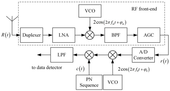
Figure 1.
Receiver model of the UAV data link.
When the receiver receives several low-power in-band and high-power out-of-band interferences, the in-band interferences will pass through the radio frequency (RF) front-end without attenuation. At the same time, the out-of-band interferences will be partially attenuated by the cavity filter of the duplexer. However, strong interferences can lead to a nonlinear effect, IM3, in the LNA. If the IM3 frequencies are within the working frequency band, the IM3 interferences can also pass through the RF front-end without attenuation. The in-band and IM3 interferences will reduce the gain of the working signal at the RF front-end and cause error bits at the data detector. When the BER exceeds the threshold, the data link will be in the loss-of-lock state.
2.2. Complex EMI Effect Assessment Model
In the complex electromagnetic environment, assume that there are q in-band and p out-of-band interferences in the additive white Gaussian noise (AWGN) channel. The modulation scheme is binary-phase shift keying (BPSK). And the data link has completed the synchronization process. The UAV receives the signal as follows:
where is the working signal with carrier frequency and amplitude . is the kth in-band interference. is the lth out-of-band interference with amplitude . is thermal noise. The phases of the working signal and interference signals at the receiver are random and statistically independent. They follow a uniform distribution over the interval [0, 2π] with an expected value of π. The phases are assumed to be π. Moreover, since the hardware remains undamaged during data link loss-of-lock, the power of thermal noise is negligible compared to the interference and can be omitted from the calculation.
After the LNA, the out-of-band interferences can generate IM3 products with in-band frequencies. In this case, both in-band and IM3 interferences are primary factors that cause the BER of the data link. In [16,19], researchers have separately studied the effect assessment models of in-band and IM3 interferences. Due to the distinct nonlinearity levels of the LNA under in-band and out-of-band interferences, their required interference energy accumulation mechanisms differ. Therefore, the assessment model for the combined interference effects cannot be formulated by the linear superposition of the two models.
Mechanistic analysis of Reference [25] indicates that the emergence of nonlinear effects in electronic components necessitates a process of energy accumulation. At the same time, the loss-of-lock fundamentally arises from the receiver’s detection of consecutive mismatches between the received codeword and the frame synchronization pattern within a unit time interval, thereby triggering a frame desynchronization response. The condition for its occurrence can be stated as follows: the number of symbols affected by the multiple interferences from the RF front-end within a unit time exceeds a predetermined threshold. Specifically, the absolute value of the total interference amplitude must surpass a preset amplitude threshold, and the duration during which the amplitude remains above this threshold must reach a specified proportion. As a result, the loss-of-lock demonstrates energy accumulation and time-delay characteristics. In summary, for a data link’s loss-of-lock, the combined amplitude fluctuation in interferences needs to satisfy the following two conditions simultaneously: over the interference period, the absolute value of the total interference amplitude exceeds a specified amplitude threshold, and the ratio of the duration during which the amplitude remains above the threshold to the total interference period is greater than a defined time–ratio threshold. Based on this, two key parameters are introduced: (1) the predefined threshold is defined as the UAV data link loss-of-lock threshold (); (2) the specified time proportion is defined as the UAV data link effect–time ratio (). Therefore, the state of the data link can be determined by assessing whether the amplitude, which makes the time proportion of the composite interference signal equal to , exceeds . Here, the amplitude is defined as the amplitude coefficient of the composite interference signal (). Furthermore, when the RF front-end outputs multiple interference signals, their superposition forms a composite interference signal. A third key parameter, the amplitude coefficient Ac, is introduced here. It is defined as the amplitude value at which the time proportion of the composite interference signal equals D. By comparing the values of and , the connectivity status of the data link can be determined. Based on the above analysis, the complex EMI effect assessment model under in-band and out-of-band interferences is given as follows:
where is the UAV data link EMI effect index. If , the data link is in the loss-of-lock state. If , the data link will work normally.
The assessment model applies to interference combinations including in-band single-tone, in-band partial-band noise, and out-of-band single-tone interferences generating in-band IM3 products. It is applicable to medium- and long-range communication links, but is not suited for extreme-proximity scenarios where the received working signal power is excessively high.
The calculation methods for the interference parameter Ac, and the data link parameters (D and At) will be elaborated on in the subsequent section.
2.3. Amplitude Coefficient Measurement Method
The amplitude coefficient needs to be calculated in real-time according to the time-varying amplitude characteristics of the composite interference signal. When contains only sinusoidal interference signals, its amplitude varies periodically, and remains constant, allowing it to be analytically calculated. However, when includes partial-band noise interference, the randomness of its amplitude makes it difficult to directly solve for . Therefore, the interference signals output from the RF front-end are classified according to their types: in-band single-tone interference and IM3 interference belong to the sinusoidal interference category, while partial-band noise interference falls into the noise interference category. To facilitate the calculation of the of the composite interference signal and to mitigate the influence of frequency-selective characteristics in the RF front-end, it is necessary to normalize the amplitude of each interference. Since the amplitude of partial-band noise interference exhibits randomness and cannot be normalized using conventional methods, its normalized amplitude is defined based on the condition that the proportion of time during which the absolute signal amplitude exceeds reaches . Let , where denotes the amplitude coefficient of the partial-band noise interference. Similarly, the normalized amplitude for sinusoidal composite interference is defined as , with being the amplitude coefficient of the sinusoidal composite interference. Furthermore, given that the operating bandwidth is much narrower than the carrier frequency and the bandwidth of the partial-band noise interference is also significantly smaller than its center frequency, the amplitude fluctuation within the bandwidth due to frequency variation is negligible. Therefore, each partial-band noise interference can be equivalently treated as a single-tone interference located at its center frequency. Similarly, all sinusoidal-type interferences can be combined into a single-tone interference at their average frequency . This equivalence holds under the key physical condition: the center frequency of any interference is significantly larger than its bandwidth (typically, a ratio greater than 150:1 is sufficient). In the long-range communication scenario considered, the carrier frequency is high, and the working bandwidth is relatively narrow. Therefore, changes in the interference frequency could have a negligible effect on amplitude variations. Based on the simplification, the normalized composite interference signal can be expressed as follows:
where and are the normalized amplitude and center frequency of the zth partial-band noise interference, respectively.
is calculated as follows:
If the sinusoidal composite interference consists of O in-band single-tone interferences and M + K IM3 interferences, let the frequency and amplitude of the oth in-band single-tone interference be and , respectively. The normalized amplitude of this in-band single-tone interference can be obtained as follows:
where denotes the interference loss-of-lock threshold when acting alone.
Suppose the kth and mth IM3 interference frequencies generated by two and three out-of-band interferences are denoted as and , respectively. The mathematical relationship between LNA nonlinear parameters and IM3 amplitude is detailed in Reference [19]. According to [19], their corresponding normalized amplitudes and are given as follows:
where is the amplitude of the working signal in the IM3 effect factor tests; is the IM3 effect factor of the Interference 1 of the kth IM3 interference, which is only frequency-dependent and can be measured; and are the real-time amplitude and loss-of-lock threshold of the Interference 1 of the kth IM3 interference, respectively. and denote the loss-of-lock threshold of the single-tone interference with frequency and , respectively. The meanings of the remaining symbols can be deduced accordingly.
By substituting , and back into their corresponding interference, the normalized sinusoidal composite interference can be expressed as follows:
The amplitude coefficient of is then computed via computer simulation, thereby yielding the by .
It should be noted that when only sinusoidal interference is present, .
is calculated as follows:
Suppose the zth partial-band noise interference occupies the frequency band [, ]. Its amplitude is random. The statistical regularity of the amplitude distribution needs to be analyzed to obtain the normalized amplitude . The single-sided power spectral density (PSD) and power of the interference are and , respectively. This interference can be regarded as the summation of many single-tone interferences, each with Gaussian-distributed amplitudes. The amplitude of the ith single-tone interference () with frequency follows a normal distribution expressed as follows:
The normalization amplitude of the single-tone interference () follows the normal distribution expressed as follows:
where is the loss-of-lock threshold (power) of the single-tone interference. Owing to the additive property of normal distributions, the amplitude of partial-band noise interference () remains normally distributed:
Discretization of the variance in Equation (9) yields, as follows:
When the partial-band noise interference acts alone, the normalization amplitude of it () follows a normal distribution given as follows:
where is the loss-of-lock threshold (single-sided PSD) of the partial-band noise interference. And the relationships between and and between the amplitude coefficient of the interference () and D can be derived from the probability distribution properties of the normal distribution as follows:
Assuming that is the two-sided D-quantile of the standard normal distribution, which can be obtained by consulting the standard normal distribution table, and can be denoted as follows:
Then, the normalized amplitude of the zth partial-band noise interference can be derived as follows:
where is the loss-of-lock threshold (power) of the zth partial-band noise interference.
Finally, the amplitude coefficient of is derived through computer simulation, combining with the calculated and .
2.4. Data Link Parameter Measurement Method
and are the key parameters for the complex EMI effect assessment model, which are fundamentally determined by the data link’s detector performance and loss-of-lock BER threshold, rather than interference types: reflects the detector’s amplitude tolerance for error-free decision-making, while D is tied to the duration required for interference to raise BER to the frame synchronization-breaking threshold. This inherent nature enables their application across diverse interferences.
Single-tone and 100% depth amplitude-modulated (AM) signals are used to measure these two parameters. This is because the single-tone signal has a constant amplitude, while the 100%-depth AM signal has a time-varying amplitude containing three single-tone signals. These two signal types have distinct characteristics and a simple implementation. The measurement method of and is as follows:
Firstly, measure the loss-of-lock thresholds of the signals, respectively: for the single-tone signal and for the AM signal. It should be noted that the single-tone signal’s frequency equals the AM signal’s carrier frequency, and the modulation frequency of the AM signal needs to be low to reduce the impact of the RF front-end’s frequency-selective characteristics.
Then, normalize the amplitudes of the signals. The normalized amplitude of the single-tone signal is , and that of the AM signal is .
Finally, compute the parameters and using a computer. Simulations are performed on the normalized-amplitude single-tone signal and AM signal using the same sampling rate. The amplitude coefficients of the two signals are the same, denoted as . By adjusting , the corresponding effect–time ratios of the two signals are obtained (, ). When , is equal to and is equal to .
3. Verification of the Model
3.1. Test Configuration
UAV data link receivers are generally housed within the fuselage interior. If UAVs have great airframe shielding performance, interference can only enter the receiver through the antenna coupling path. In this case, the EMI injection test method and the radiated susceptibility test method are equivalent [26,27]. The EMI injection test method was employed for its cost-efficiency, high repeatability, and accuracy. The test configuration is shown in Figure 2. The working signal and interferences are combined by a combiner into a single path and then injected into the receiver and a spectrum analyzer. The test configuration mainly contains three modules: the test object module (gray), the interference generation module (red), and the monitor module (yellow).
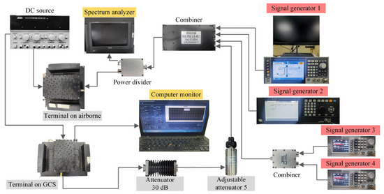
Figure 2.
Test configuration.
The test object is a certain type of DSSS-based data link consisting of the data link terminal on airborne and the data link terminal on GCS. The carrier frequency of the working signal is (L-band), and the bandwidth is 10 MHz. The adjustable attenuator 5 and the 30 dB attenuator are used to simulate the attenuation caused by the flight distance.
The interference generation module is composed of signal generators. A signal generator generates an interference. The signal generators (1–4) used in this study are R&S SMBV100B, Sinolink SLVS12A, and two RIGOL DSG821.
In the monitor module, the computer monitor provides real-time metrics of the data link, including BER and synchronization lock status, and the spectrum analyzer provides the received signal power.
3.2. Single-Source EMI Injection Effect Tests
The loss-of-lock thresholds of interferences and the parameters ( and ) were measured using the single-source EMI injection effect tests. The test configuration is shown in Section 3.1, using signal generator 1 to generate interference. The test procedure is as follows:
Step 1. Adjustable attenuator 1 is set according to the required working signal power at the receiver input. Set signal generator 1 according to the interference parameters. The initial output power is set to a low level.
Step 2. Using an adjustable pace method, gradually increase the output power of signal generator 1 until the data link loses lock.
Step 3. Reduce the output power by 3 dB. Repeat Step 2. Record the final interference power as the loss-of-lock threshold of the interference.
Setting , the test loss-of-lock threshold curve is shown in Figure 3. The data link is highly sensitive to in-band interference within a frequency offset () range from −5 MHz to 5 MHz. refers to the interference frequency minus the working signal carrier frequency. The loss-of-lock threshold increases as the absolute value of the frequency offset increases. In contrast, the data link demonstrates low sensitivity to out-of-band interference, showing higher loss-of-lock thresholds and a small frequency-dependent manner. The interference loss-of-lock thresholds can be obtained by tests or machine-learning algorithms as the foundation for assessing complex EMI effects.
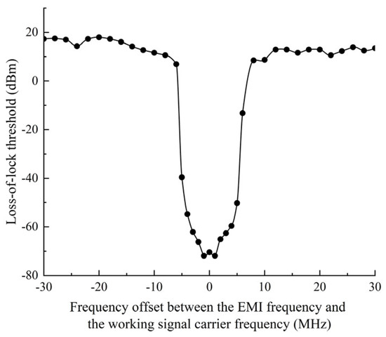
Figure 3.
The loss-of-lock threshold curves of single-tone interference at a working signal power of −89 dBm.
3.3. Data Link Parameter Tests
To assess the complex EMI effects in this study, parameters , , and IM3 effect factor are required. According to Section 2.4, the loss-of-lock thresholds of single-tone and 100% depth AM signals need to be tested, the results of which are shown in Figure 4. Figure 4a presents the loss-of-lock thresholds under different when . The loss-of-lock thresholds for AM signals are lower than those for single-tone signals. This means that the data link is more susceptible to the AM interference. Figure 4b shows the thresholds at under varying working signal powers, which reveals nearly parallel threshold curves, suggesting that the difference between their loss-of-lock thresholds remains relatively constant regardless of working signal power variations in the range from −99 dBm to −49 dBm. Figure 4c indicates the critical power of single-tone and AM signals under different BER, at and , −69 dBm, and −49 dBm. As the BER increases, the critical power also increases. The trend of critical power is consistent under different working signal powers. As the BER increases, the power difference between the single-tone and AM signals decreases.
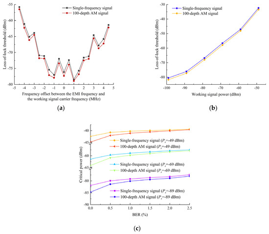
Figure 4.
Test results of single-tone and 100% depth AM signal parameter testing. (a) Loss-of-lock threshold versus frequency offset at a working signal power of −89 dBm; (b) loss-of-lock threshold versus working signal power at 0 MHz frequency offset; (c) critical power versus BER at 0 MHz frequency offset under working signal powers of −89 dBm, −69 dBm, and −49 dBm.
After amplitude normalization and computer calculations, the results of and are shown in Figure 5. Figure 5a presents the results of and under different at . These two parameters fluctuate less with frequency and are negatively correlated. This is because, for a normalized signal, a larger D requires a smaller to increase the time proportion of signal amplitudes exceeding the threshold within a signal cycle. The standard deviations of and across all in-band frequencies are 0.0065 and 0.016, respectively, demonstrating strong consistency, with mean values of 0.964 for and 0.171 for .
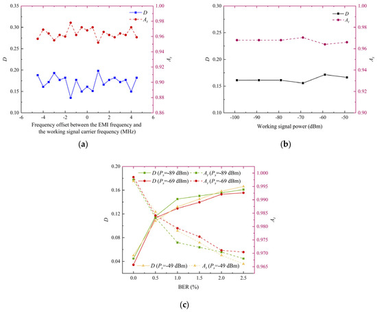
Figure 5.
Results of parameters At and D. (a) Parameters versus frequency offset at a working signal power of −89 dBm; (b) parameters versus working signal power at 0 MHz frequency offset; (c) parameters versus BER at 0 MHz frequency offset under working signal powers of −89 dBm, −69 dBm, and −49 dBm.
Figure 5b shows the results under different working signal powers at . The parameters are almost constant under the working signal power range of −99 dBm to −49 dBm.
Figure 5c indicates the results under different BER at and different . As BER increases, increases and exhibits a decreasing trend. As the BER increases, indicating increased allowable errors of the demodulator per unit time, an increase in D and a decrease in are needed. As shown in Figure 5, the parameters and D of the data link are mainly related to the data link’s loss-of-lock criterion, which is governed by the BER threshold. Notably, and D are intrinsic properties of the data link. They can be determined, either by the experimental–simulation method described in Section 2.4, or by developing a machine-learning-based prediction model (e.g., using XGBoost or neural networks).
The IM3 effect factors at various frequency points of the data link have been measured in [19] with the test working signal power of −87 dBm. The IM3 effect factor curves are shown in Figure 6. Figure 6a and b show the IM3 effect factors of the frequencies with negative and positive frequency offsets, respectively.
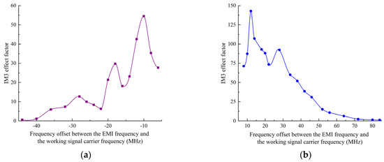
Figure 6.
The IM3 effect factor curve. (a) Negative frequency offset frequency points; (b) positive frequency offset frequency points.
3.4. Three-Source EMI Injection Effect Tests
To verify the accuracy of the complex EMI effect assessment model, three-source EMI injection effect tests were conducted. According to Section 3.1, the signal generators 1–3 were used. The test procedure is as follows:
Step 1. Each signal generator’s output power is individually set according to the loss-of-lock threshold of the interference.
Step 2. Reduce the power of the interferences. The power of the in-band and the out-of-band interferences is reduced by 6 dB and 45 dB, respectively.
Step 3. Increase all three interference powers using the alterable pace method. When the data link loses lock, the power of one of the interferences is reduced by 3 dB. Then, increase this interference power until loss-of-lock recurrence. Record these three interference powers.
Based on the above test procedure, three-source EMI injection effect tests were conducted using one in-band interference (Interference 1) and two out-of-band interferences (Interference 2 and 3). Interferences 2 and 3 generated an IM3 interference with an in-band frequency. The tests comprised four main groups containing three subgroups with different interference power combinations. In group 1, there were three single-tone interferences with of 1 MHz, 8 MHz, and 16 MHz. In group 2, there were three single-tone interferences with of −1 MHz, −10 MHz, and −20 MHz. In group 3, the interferences comprised: (1) one partial-band noise interference with (the center frequency minus the working carrier frequency) of 0 MHz and bandwidth of 2 MHz; (2) two single-tone interferences with of 14 MHz and 26 MHz. In group 4, the interferences consisted of a partial-band noise interference with of −1.5 MHz and bandwidth of 5 MHz, and two single-tone interferences with of −6 MHz and −14 MHz. The working signal power was set to −89 dBm. The test and calculation results of these four groups are shown in Table 1. Table 1 presents the normalized power of each interference, the normalized amplitude of sinusoidal composite interference () and partial-band noise interference (), and the effect index (). The theoretical value of is 1 (0 dB), and the test values range up to a maximum of 1.177 (0.709 dB) and a minimum of 0.989 (−0.05 dB). The maximum difference between the theoretical and test results is 0.709 dB, demonstrating that the assessment model has high accuracy.

Table 1.
Test data and effect index of three-source EMI injection effect tests.
Groups 1-1, 2-1, 3-1, and 4-1 were selected for validation tests. The power of Interference 2 in each subgroup was increased by 1 dB and decreased by 1 dB, respectively. The validation test results are shown in Table 2. When , the data link is in loss-of-lock status. Conversely, when , the data link remains synchronized.
Table 2.
Effect index of three-source EMI injection validation tests.
3.5. Four-Source EMI Injection Effect Tests
Four-source EMI injection effect tests were conducted to validate the assessment model’s applicability further. The test configuration remained consistent with Section 3.1, and the test procedure followed the three-source EMI injection effect test procedure, with the addition of signal generator 4.
Four-source EMI injection effect tests contained five groups, each containing three subgroups. The working signal power was set to −89 dBm. Table 3 shows the four interference configurations and frequency offsets between the IM3 frequency and for each group. The interference configurations contain multiple interference types: single-tone interference, partial-band noise interference, one IM3 interference generated by three and two out-of-band interferences, and two IM3 interferences produced from three out-of-band interferences.
Table 3.
Interference configurations of four-source EMI injection effect tests.
Table 4 summarizes the test results for the five groups. As shown in Table 4, the maximum and minimum values of the effect index are 0.905 and 1.159, respectively. The error to the theoretical value is less than 0.64 dB, further demonstrating the assessment model’s good accuracy and applicability under the complex EMI.
Table 4.
Test data and effect index of four-source EMI injection effect tests.
The first subgroup of each group was selected for validation tests. The power of Interference 2 in each subgroup was increased and decreased by 1 dB, respectively, to observe the data link’s working status. The results are summarized in Table 5. When , the data link loses lock. When , the data link’s synchronization is normal. However, in a limited number of instances, the model yielded false alarms. This occurred when the data link did not experience an actual loss-of-lock despite a calculated , as observed in Group 5-1-1. The root cause of this single false alarm was a minor mismatch between model simplifications and actual conditions. This arose from two factors: instantaneous phase cancelation among interferences; and slight dynamic fluctuations in LNA nonlinearity. The latter caused the third-order nonlinear coefficient to deviate from the measured IM3 effect factor, resulting in a lower actual IM3 amplitude than predicted. These led to the false alarm.
Table 5.
Effect index of four-source EMI injection validation tests.
The three-source and four-source tests encompass complex interference combinations with cross-band and intermodulation effects, including two out-of-band single-tones generating one in-band IM3 product, three out-of-band single-tones generating two in-band IM3 products, in-band single-tone interferences, and in-band partial-band noise interferences, which configurations reflect typical complex EMI scenarios in battlefields to a certain extent.
The results of three-source and four-source EMI injection effect tests indicate that the maximum error between the experimental and theoretical values of is 0.709 dB, which is less than 1.5 dB. The validation tests reveal: when , the UAV data link is in the loss-of-lock status. When , the UAV data link remains locked. These demonstrate the assessment model’s accuracy and practical applicability.
4. Assessment Process of Complex EMI Effects on UAV Data Links
4.1. Complex EMI Effect Division
Based on the different states of a data link, its working status is classified into four states: loss-of-lock state, quasi-loss-of-lock state, quasi-safe state, and safe state [17]. Correspondingly, the complex EMI effect index from Section 2.2 is stratified into three levels: first-level effect index , second-level effect index , and third-level effect index . As the interference amplitude decreases across the four states, need to be reduced in the three critical states. The three effect indexes are denoted as follows:
where and are first-level and second-level safety margins, both bigger than 1, and . Specifically, and are set to 1.413 and 1.995, respectively [28]. The two margins directly affect state classification sensitivity. and can be adaptively configured by mission requirements: high-priority tasks (e.g., reconnaissance) may adopt larger values (e.g., , ) for earlier warnings, routine tasks use the baseline (e.g., , ) to balance safety and operational continuity, and low-risk civilian scenarios (e.g., aerial surveying) may reduce values (e.g., , ) to minimize redundant alerts.
Then, the state is determined as follows:
4.2. Complex EMI Effect Assessment Process
In practical applications, a UAV employs an EMI sensing system to detect interference characteristics and the assessment results to make anti-interference strategies. The sensing system shares the same antenna with the data link receiver. The assessment process is shown in Figure 7. Suppose that the Gaussian channel contains one in-band partial-band noise interference (Interference 1) and two out-of-band interferences (Interference 2 and 3) which generate an in-band IM3 product. Set and . The assessment process for this scenario is shown as follows:
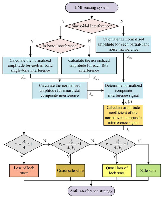
Figure 7.
Complex EMI effect assessment process.
Step 1. The interference sensing system identifies the center frequencies as , MHz, MHz, with corresponding bandwidths MHz, MHz, MHz and powers dBm, dBm, and dBm. Classify the interferences into noise and sinusoidal interference based on bandwidth, and classify the sinusoidal interferences into in-band and out-of-band interference based on frequency. The third-order intermodulation product frequency generated by the out-of-band interferers is calculated as MHz.
Step 2. Normalize the amplitude of the IM3 interference , and then calculate the normalized amplitude of sinusoidal composite interference . Moreover, calculate the normalized amplitude of the partial-band noise interference . The normalized composite interference signal is then expressed as .
Step 3. The amplitude coefficient Ac of the signal is computed as through computer simulation.
Step 4. Using Equation (17), obtain , , and . According to the criterion in Equation (18), since , the data link is judged to be in the loss-of-lock state.
Step 5. Feed the state to the anti-interference strategy system for real-time countermeasure deployment (e.g., frequency hopping, power adjustment) [17]. The following are example anti-interference strategies corresponding to each state:
Safe state: Maintain current working parameters to avoid unnecessary energy consumption.
Quasi-safe state: Moderately increase the working signal’s transmit power, switch to preloaded low-interference frequency bands, or activate beam-forming and beam-tracking techniques.
Quasi-loss-of-lock state: Employ beam-forming and beam-tracking, while simultaneously adjusting the UAV’s flight attitude or trajectory.
Loss-of-lock state: Initiate the UAV’s autonomous return protocol: command it to fly back along the original flight path to the nearest interference-free zone, preventing complete loss of communication control.
Unlike the models in [16,17], the proposed model encompasses combined interference environments, including in-band single-tone, in-band partial-band noise, and out-of-band sources that generate in-band IM3 products. This capability allows it to better represent the complex, heterogeneous EMI of real battlefields and offers broader utility for UAV data link assessment.
5. Conclusions
This study proposes a complex EMI effect assessment model to improve the anti-interference ability of UAV data links. The model is applicable to scenarios involving in-band single-tone, partial-band noise, and third-order intermodulation (IM3) interferences. Its validity was successfully demonstrated through tests. The main conclusions are as follows:
- By analyzing the energy accumulation characteristics of nonlinear effects and the time-delay characteristics of the loss-of-lock effect, three key parameters are proposed. These are the UAV data link loss-of-lock threshold , the effect–time ratio D, and the effect index τ. A complex EMI effect assessment model is established based on these parameters. And the calculation method of and D is introduced. The model applies to the complex EMI scenarios involving in-band single-tone, partial-band noise, and out-of-band single-tone interferences generating in-band IM3 interferences.
- The measured values for and D of the tested are approximately 0.964 and 0.171, respectively. A key finding is the inverse correlation between and D. Furthermore, both parameters are linked to the data link’s loss-of-lock criterion, governed by the BER. Specifically, as the BER decreases, decreases, and D increases.
- The model’s accuracy and applicability are verified through three-source and four-source EMI injection effect tests. The test results of range from 0.905 to 1.177, with a maximum deviation of 0.709 dB from the theoretical value of 1 (0 dB). This demonstrates the model’s high predictive accuracy. The validation tests further confirm that the data link loses lock when and maintains synchronization when .
- To enable more refined state discrimination, a three-level effect index (, , and ) is introduced, categorizing the data link status into four distinct states.: Loss-of-lock state: Quasi-loss-of-lock state: Quasi-safe state: Safe state
In future work, we will further study the effect assessment of out-of-band partial-band noise and out-of-band non-intermodulation interferences, verify the model with more complex suppressive interferences (e.g., AM interference, comb-spectrum interference), and introduce a dynamic phase correction factor and a dynamic LNA nonlinearity compensation model. These will broaden the model’s applicability to more realistic complex electromagnetic environments to broaden the model’s application scenarios and provide further theoretical support for UAVs to realize intelligent anti-interference decision-making in complex electromagnetic environments.
Author Contributions
Conceptualization, X.Z.; methodology, X.Z.; software, X.Z.; validation, X.Z.; formal analysis, X.Z.; investigation, X.Z.; resources, Y.C.; data curation, X.Z.; writing—original draft preparation, X.Z.; writing—review and editing, X.Z. and Y.C.; visualization, Y.S. and Y.W.; supervision, Y.C.; project administration, Y.C. and M.Z.; funding acquisition, Y.C. and M.Z. All authors have read and agreed to the published version of the manuscript.
Funding
This research was funded by the National Natural Science Foundation of China (Grant No. 62301605) and the National Defense Basic Scientific Research Program of China (Grant No. JCKYS2023DC01).
Data Availability Statement
All data supporting the findings of this study are included in this article.
Conflicts of Interest
The authors declare no conflicts of interest.
Abbreviations
The following abbreviations are used in this manuscript:
| UAV | Unmanned Aerial Vehicle |
| EMI | Electromagnetic Interference |
| GCS | Ground Control Station |
| HPM | High-Power Microwave |
| GPR | Gaussian Process Regression |
| SSA-DCNN | Sparrow Search Algorithm–Dual-Channel Convolutional Neural Network |
| MIMT-CNN | Multi-Task Convolutional Neural Network with Multi-Input |
| IM3 | Third-Order Intermodulation |
| BER | Bit Error Rate |
| DSSS | Direct Sequence Spread Spectrum |
| RF | Radio Frequency |
| LNA | Low Noise Amplifier |
| PSD | Power Spectral Density |
| AM | Amplitude-Modulated |
References
- Bao, B.; Luo, C.; Hong, Y.; Chen, Z.; Fan, X. High-Precision UAV Positioning Method Based on MLP Integrating UWB and IMU. Tsinghua Sci. Technol. 2025, 30, 1315–1328. [Google Scholar] [CrossRef]
- Lv, J.; Cheng, J.; Li, P.; Bai, R. Secure energy efficiency maximization for mobile jammer-aided UAV communication: Joint power and trajectory optimization. Veh. Commun. 2025, 53, 100910. [Google Scholar] [CrossRef]
- Wang, D.; Rong, R.; Li, G. Coverage-Optimal UAV Deployment and Energy-Efficient Sensor Power Allocation for UAV-Enabled Data Collection. J. Commun. Inf. Netw. 2025, 10, 50–56. [Google Scholar] [CrossRef]
- Wang, X.; Guo, H.; Wang, J.; Wang, L. Predicting the Health Status of an Unmanned Aerial Vehicles Data-Link System Based on a Bayesian Network. Sensors 2018, 18, 3916. [Google Scholar] [CrossRef]
- Wang, H.; Ding, G.; Chen, J.; Zou, Y.; Gao, F. UAV Anti-Jamming Communications With Power and Mobility Control. IEEE Trans. Electromagn. Compat. 2023, 22, 4729–4744. [Google Scholar] [CrossRef]
- Yin, Z.; Li, J.; Wang, Z.; Qian, Y.; Lin, Y.; Shu, F.; Chen, W. UAV Communication Against Intelligent Jamming: A Stackelberg Game Approach With Federated Reinforcement Learning. IEEE Trans. Green Commun. Netw. 2024, 8, 1796–1808. [Google Scholar] [CrossRef]
- Jie, H.; Zhao, Z.; Zeng, Y.; Chang, Y.; Fan, F.; Wang, C.; See, K.Y. A review of intentional electromagnetic interference in power electronics: Conducted and radiated susceptibility. IET Power Electron. 2024, 17, 1487–1506. [Google Scholar] [CrossRef]
- Lan, X.; Tang, X.; Zhang, R.; Li, B.; Wang, Y.; Niyato, D.; Han, Z. UAV-Assisted Integrated Communication and Over-the-Air Computation With Interference Awareness. IEEE Trans. Commun. 2025, 73, 10647–10661. [Google Scholar] [CrossRef]
- Ibeobi, S.; Pan, X. A New Approach for Error Rate Analysis of Wide-Band DSSS-CDMA System with Imperfect Synchronization Under Jamming Attacks. Wirel. Pers. Commun. 2021, 98, 44–53. [Google Scholar] [CrossRef]
- Luo, X.; You, L.; Lv, J.; Chen, Z. Multidomain Narrowband Interference Intelligent Suppression Method Based on Cognitive Radio and MIMO in UAV Data Link. Comput. Intell. Neurosci. 2022, 2022, 6207937. [Google Scholar] [CrossRef]
- Ibeobi, S.; Pan, X. Study of electromagnetic pulse (EMP) effect on surveillance unmanned aerial vehicles (UAVs). J. Mech. Eng. Autom. Control Syst. 2021, 2, 44–53. [Google Scholar] [CrossRef]
- Mao, Q.; Xiang, Z.; Huang, L.; Meng, J.; Wang, H.; Yang, C.; Cui, Y. High-Power Microwave Pulse-Induced Failure on Unmanned Aerial Vehicle System. IEEE Trans. Plasma Sci. 2023, 51, 1885–1893. [Google Scholar] [CrossRef]
- Zhang, Z.; Zhou, Y.; Zhang, Y.; Qian, B. Investigation on the effects of C-band high-power microwave on unmanned aerial vehicle system. J. Electromagn. Waves Appl. 2025, 39, 476–489. [Google Scholar] [CrossRef]
- Cai, S.; Li, Y.; Zhu, H.; Wu, X.; Su, D. A Novel Electromagnetic Compatibility Evaluation Method for Receivers Working under Pulsed Signal Interference Environment. Appl. Sci. 2021, 11, 9454. [Google Scholar] [CrossRef]
- Xu, T.; Chen, Y.; Wang, Y.; Zhang, D.; Zhao, M. EMI Threat Assessment of UAV Data Link Based on Multi-Task CNN. Electronics 2023, 12, 1631. [Google Scholar] [CrossRef]
- Li, W.; Wei, G.; Pan, X.; Wan, H.; Lu, X. Electromagnetic Compatibility Prediction Method Under the Multifrequency in-Band Interference Environment. IEEE Trans. Electromagn. Compat. 2018, 60, 520–528. [Google Scholar] [CrossRef]
- Zhang, X.; Chen, Y.; Zhao, M.; Li, Y. Assessment of EMI Effects on UAV Data Links. IEEE Trans. Electromagn. Compat. 2025, 67, 786–799. [Google Scholar] [CrossRef]
- Du, X.; Wei, G.; Pan, X.; Wan, H.; Zhao, H. Study on the Law and Mechanism of the Third-Order Intermodulation False Alarm Effect of the Stepped Frequency Ranging Radar. Electronics 2022, 11, 3722. [Google Scholar] [CrossRef]
- Zhang, X.; Zhao, M.; Chen, Y. Prediction of Third-Order Intermodulation Effects from Out-of-Band Electromagnetic Interference in UAV Data Links. Acta Armamentarii 2025. [Google Scholar] [CrossRef]
- Wang, P.; Ma, K.; Bai, Y.; Sun, C.; Wang, Z.; Chen, S. Wireless Interference Recognition With Multimodal Learning. IEEE Trans. Wirel. Commun. 2024, 23, 18576–18591. [Google Scholar] [CrossRef]
- Wang, P.; Cheng, Y.; Dong, B.; Hu, R.; Li, S. WIR-Transformer: Using Transformers for Wireless Interference Recognition. IEEE Wirel. Commun. Lett. 2022, 11, 2472–2476. [Google Scholar] [CrossRef]
- Xu, H.; Cheng, Y.; Liang, J.; Wang, P. A Jamming Recognition Algorithm Based on Deep Neural Network in Satellite Navigation System. In Lecture Notes in Electrical Engineering; Springer: Singapore, 2020; pp. 701–711. [Google Scholar] [CrossRef]
- Zhao, H.; Sun, F.-Y.; Cai, Y.; Liu, W.-K. A Time–Frequency Energy Squeeze Method Based on Estimating the Chip Rate of DSSS Signals. Sensors 2025, 25, 596. [Google Scholar] [CrossRef]
- Lu, Q.; He, F.; Wang, Z.; Ma, Y.; Yang, Z.; Li, Y.; Wu, H.; Li, W. Performance Analysis for DSSS With Short Period Sequences Encountering Broadband Interference. IEEE Trans. Veh. Technol. 2024, 73, 16697–16710. [Google Scholar] [CrossRef]
- Zhang, Q.; Wang, Y.; Cheng, E.; Ma, L.; Chen, Y. Investigation on the Effect of the B1I Navigation Receiver Under Multifrequency Interference. IEEE Trans. Electromagn. Compat. 2022, 64, 1097–1104. [Google Scholar] [CrossRef]
- Lu, X.; Wei, G.; Pan, X. A double differential-mode current injection method based on directional couplers for HIRF verification testing of interconnected systems. J. Electromagn. Waves Appl. 2014, 28, 346–359. [Google Scholar] [CrossRef]
- GJB8848–2016; Electromagnetic Environment Effects Test Methods for Systems. Wuhan Detech Technology Co., Ltd.: Wuhan, China, 2016.
- GJB151B–2013; Electromagnetic Emission and Susceptibility Requirements and Measurements for Military Equipment and Subsystems. Beijing COC Tech Co., Ltd.: Beijing, China, 2013.
Disclaimer/Publisher’s Note: The statements, opinions and data contained in all publications are solely those of the individual author(s) and contributor(s) and not of MDPI and/or the editor(s). MDPI and/or the editor(s) disclaim responsibility for any injury to people or property resulting from any ideas, methods, instructions or products referred to in the content. |
© 2025 by the authors. Licensee MDPI, Basel, Switzerland. This article is an open access article distributed under the terms and conditions of the Creative Commons Attribution (CC BY) license (https://creativecommons.org/licenses/by/4.0/).