A Real-Time Photovoltaic Power Estimation Framework Based on Multi-Scale Spatio-Temporal Graph Fusion

Abstract

Accurate forecasting of photovoltaic (PV) power is crucial for real-time grid balancing and storage optimization. However, the intermittent, noisy, and nonstationary nature of PV generation, together with cross-site interactions, makes multi-site intra-hour forecasting challenging. In this paper, we propose a unified approach for multi-site PV power forecasting named WGL (Wavelet–Graph Learning). Unlike prior studies that treat denoising and spatio-temporal modeling separately or predict each station independently, WGL forecasts all PV stations jointly while explicitly capturing their inherent spatio-temporal correlations. Within WGL, Learnable Wavelet Shrinkage (LWS) performs end-to-end noise suppression; a Temporal Multi-Scale Fine-grained Fusion (T-MSFF) module extracts complementary temporal patterns; and an attention fusion gate adaptively balances TCN and LSTM branches. For spatial coupling, graph self-attention (GSA) learns a sparse undirected graph among stations, and a Factorized Spatio-Temporal Attention (FSTA) efficiently models long-range interactions. Experiments on real-world multi-site PV datasets show that WGL consistently outperforms representative deep and graph-based baselines across intra-hour horizons, highlighting its effectiveness and deployment potential. Furthermore, a comprehensive analysis of influencing factors for scheme implementation—encompassing safety, reliability, economic rationality, management scientificity, and humanistic care—is conducted, providing a holistic assessment of the framework’s feasibility and potential impact in real-world power systems.

1. Introduction

With the accelerating integration of renewable energy into modern power grids, photovoltaic (PV) generation, a leading clean energy technology, has become one of the most variable and least predictable elements within the system. The power output of PV systems is determined by a complex interplay of meteorological conditions, solar irradiance, ambient temperature, module characteristics, and operational and maintenance factors. As a result, PV power demonstrates significant temporal nonlinearity and nonstationarity, alongside spatial patterns marked by pronounced regional interdependencies [1]. Consequently, accurately modeling the spatio-temporal dependencies of PV power from multi-source heterogeneous data has emerged as a critical frontier in smart grid analytics and renewable energy forecasting.

Early efforts in PV power forecasting predominantly employed statistical and physical models, including ARIMA, Kalman filters, and numerical weather prediction (NWP) correction frameworks [2,3,4,5]. Böök et al. (2020) developed a site-specific bias-correction method using measured plant data to adjust NWP-based forecasts, showing that physical models require statistical calibration to suppress observational noise and systematic bias [6]. Yang et al. (2021) integrated Kalman filtering, NWP, and empirical techniques, revealing that models trained solely on historical data tend to degrade under anomalous weather conditions, and that Kalman-based frameworks exhibit heightened sensitivity to the specification of observational noise [4]. Consequently, these approaches typically assume stationarity, limiting their ability to capture strong nonlinear dynamics and leaving them vulnerable to meteorological variability and measurement noise.

Within the deep learning paradigm, PV power modeling has moved beyond isolated “single-station time series” toward spatio-temporal collaboration. Early work captured temporal dependencies using CNNs, RNNs, LSTMs, and TCNs [7,8,9,10]. Campos et al. (2024) showed with LSTM that gating alleviates RNN gradient vanishing and enables long-range dependence modeling [11]. Chu et al. (2024) reviewed the field and noted a persistent bias toward single-point or purely temporal studies [12]. Ait Mouloud et al. (2025) proposed a Q-CNN-GRU seasonal quantile framework that outperformed baselines across regions, seasons, and horizons, validating CNN–RNN hybrids for complex dynamics [13]. Wang et al. (2025) introduced ETCN and found that joint temporal–spatial modeling markedly improves accuracy, underscoring the limitations of single-station approaches [14].

Collectively, LSTM demonstrates superior capability in capturing long-range temporal dependencies, while TCN offers notable advantages for short and medium term forecasting owing to its parallel computation and stable gradient propagation. Nevertheless, the majority of existing approaches remain restricted to single-site or purely temporal modeling, which hinders their ability to represent spatial dependencies and geographical correlations among PV plants, ultimately constraining predictive accuracy. To more effectively represent spatial structures across multiple sites, recent studies have increasingly employed Graph Neural Networks (GNNs) and their spatio-temporal extensions [15,16]. Within these frameworks, power plants, measurement sites, and meteorological variables are modeled as nodes, while edges—defined by geographic proximity, electrical connectivity, or irradiance-field similarity—encode the spatial topology. Conventional Graph Convolutional Networks (GCNs) propagate and aggregate node features through spectral or spatial filtering and message passing, thereby facilitating cross-regional information exchange [17]. Building upon this foundation, Zang et al. [18] proposed an adaptive adjacency mechanism integrated with temporal convolution to achieve end-to-end multi-site irradiance forecasting, eliminating the dependence on predefined priors and consistently outperforming multiple baseline models. Attention mechanisms have further advanced spatio-temporal graph models, such as GSTANN and STGANet [19,20], by enabling networks to learn interaction strengths through trainable attention weights. Subsequent studies have introduced dynamic attention combined with error correction [21], ultra-short-term dependency learning that surpasses conventional time-series baselines [22], and Fourier-domain graph convolution to further enhance multi-site forecasting performance [23].

Although significant progress has been made, conventional Graph Neural Networks (GNNs) continue to depend on predefined or quasi-static adjacency structures, which restrict their adaptability to dynamic and time-varying correlations. As the number of nodes increases or the graph topology becomes more complex, the computational and memory demands of attention and graph convolution rise sharply, posing substantial scalability challenges for near-real-time forecasting across large-scale photovoltaic (PV) networks [24]. At the same time, multi-source data fusion has emerged as a crucial approach for enhancing the robustness of PV power forecasting. The integration of multi-scale meteorological datasets, including satellite remote sensing, numerical weather prediction (NWP), and ground-based observations, improves spatio-temporal resolution and enables the synergistic combination of high-precision local signals with large-scale meteorological trends, thereby reducing the uncertainty inherent in single-source data [25,26]. However, inconsistencies in temporal alignment, spatial coverage, and noise characteristics often render direct fusion redundant or mutually interfering. These limitations have motivated the development of multi-scale decomposition and feature reconstruction techniques, such as Wavelet Transform (WT) and Empirical Mode Decomposition (EMD), to separate smooth trends from rapid fluctuations across multiple frequency bands [27,28]. Despite substantial progress in temporal sequence modeling, spatial correlation learning, and data fusion, several critical challenges remain to be addressed.

Multi-source inputs are often noisy and nonstationary, impairing stable feature extraction and model generalization; PV output exhibits multi-scale temporal dynamics (minute, hourly, diurnal) that create complex dependencies; and strong inter-plant spatial correlations are difficult for conventional models to capture under constrained computation, limiting high-dimensional spatial representation. To tackle these issues, we propose a spatio-temporal graph deep learning framework that fuses multi-source data and employs a modular hierarchy for end-to-end denoising, spatio-temporal feature fusion, and spatial relationship modeling.

(1)

A Learnable Wavelet Shrinkage (LWS) module is designed to enable end-to-end denoising and feature purification, preserving the advantages of time–frequency localization while adaptively tuning threshold parameters.

(2)

A Temporal Multi-Scale Fine-Grained Fusion (T-MSFF) mechanism is proposed, integrating the complementary strengths of LSTM and TCN for capturing long-term dependencies and local temporal dynamics. In addition, an adaptive Attention Fusion strategy assigns importance weights to features across multiple temporal scales.

(3)

By incorporating Graph Self-Attention and Factorized Spatio-Temporal Attention (FSTA), the framework effectively captures geometric priors among PV stations while mitigating computational complexity, thereby enabling efficient cross-node interaction and dynamic dependency learning.

2. Methods

2.1. Problem Statement

In this study, we cast the problem as an ultra-short-term, multi-step photovoltaic (PV) power forecasting task. The model ingests the past 12 h of historical power data and predicts total PV output at future horizons using deep learning (Figure 1). Modeling historical sequences enables robust forecasting under incomplete or anomalous conditions, thereby enhancing the accuracy and resilience of real-time situational awareness.

2.2. Data Analysis

This study conducts an empirical analysis based on multi-site photovoltaic (PV) generation data collected from various locations across Greece. The dataset serves as both the primary analytical corpus and the benchmark reference, consisting of hourly grid-connected time series data from three PV plants, with representative geographic coordinates detailed in

Table 1. Photovoltaic station ID and its representative latitude–longitude coordinates.

id1	representative_lat	representative_lon
11381	′37.93764758004892	′23.94672727600173
12936	′36.90343810279575	′22.59962975217044
13673	′36.88173702884734	′22.61182776738177

. The observation period spans from 1 January 2017 to 31 December 2020 at an hourly resolution, encompassing four full years and capturing pronounced seasonal and interannual variability. To ensure comparability, all sites were temporally aligned and subjected to standard quality-control procedures. On this basis, we adopted a unified sliding-window sampling strategy for multi-step forecasting and cross-site modeling. This configuration facilitates both single-site performance evaluation and analysis of inter-site spatio-temporal dependencies influencing forecasting accuracy.

Additionally, to further evaluate the generalization capability of the proposed model, we collected hourly power generation time series from 12 wind farms in the same region of Greece using a similar data acquisition methodology. Representative geographic coordinates for these sites are listed in

Table 2. Wind farm ID and its representative latitude–longitude coordinates.

id1	representative_lat	representative_lon
32947	′38.77495228355805	′20.99343094669421
33332	′37.48529591563293	′23.15524708402554
33466	′38.47847602525017	′23.31767056640640
33629	′37.53446386024317	′22.59745692645553
33647	′41.05658631442512	′26.01365802179738
33651	′39.77489308387599	′20.54836510628408
33652	′39.83657134611421	′20.51975059921616
33714	′38.31711222262845	′22.93118749024237
33804	′38.31357150723943	′22.58156584100527
33805	′37.69128267903497	′22.45947529645754
33815	′37.39645464791498	′22.36230124266805
33827	′37.47515178957543	′23.92618336616106
33837	′38.23349790973124	′23.49681071356205
34105	′38.29735981237283	′20.51236928046155
34391	′38.24453603697121	′23.11726008655046
34398	′41.15301647565505	′25.83573847781144
34443	′41.28636711562325	′25.90458879167402
36876	′38.76934867818434	′21.23292614841204

.

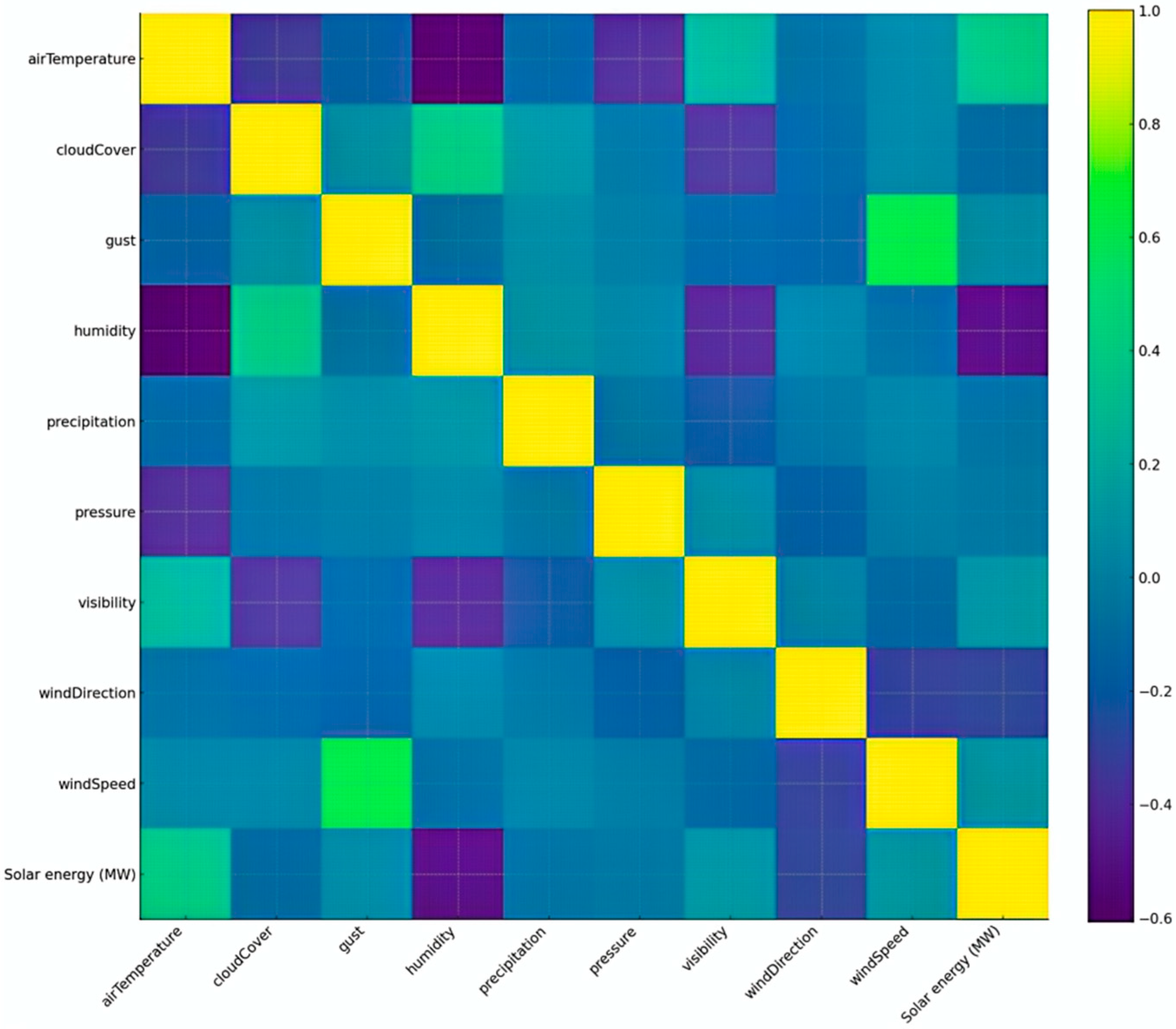
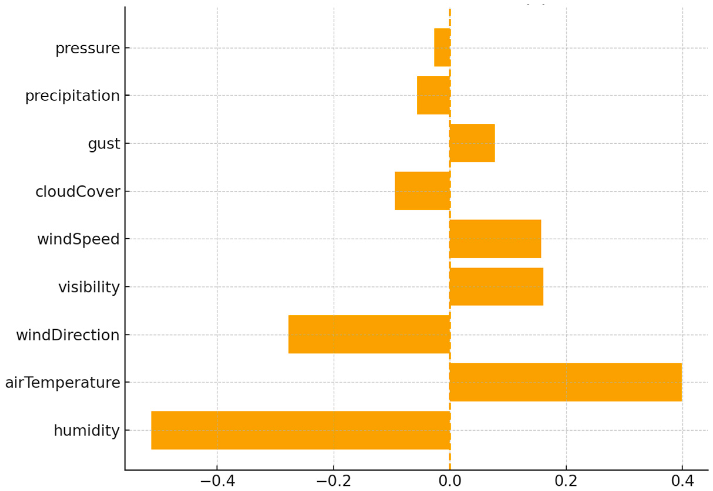
As shown in Figure 2 and Figure 3, the results of the comprehensive Pearson correlation analysis and heatmap visualization consistently indicate that the meteorological variables most strongly correlated with PV power generation are air temperature (r ≈ 0.4–0.5, positive correlation) and humidity (r ≈ −0.5, negative correlation). Following these, wind direction exhibits a moderate negative correlation (r ≈ −0.28), while wind speed and visibility show weak to moderate positive correlations (r ≈ 0.1–0.3). In contrast, cloud cover displays a weak negative correlation (r ≈ −0.1 to −0.2), gust speed a weak positive correlation (r ≈ 0.08), and both precipitation (r ≈ −0.05) and atmospheric pressure (r ≈ −0.02) demonstrate very weak correlations with PV power output.

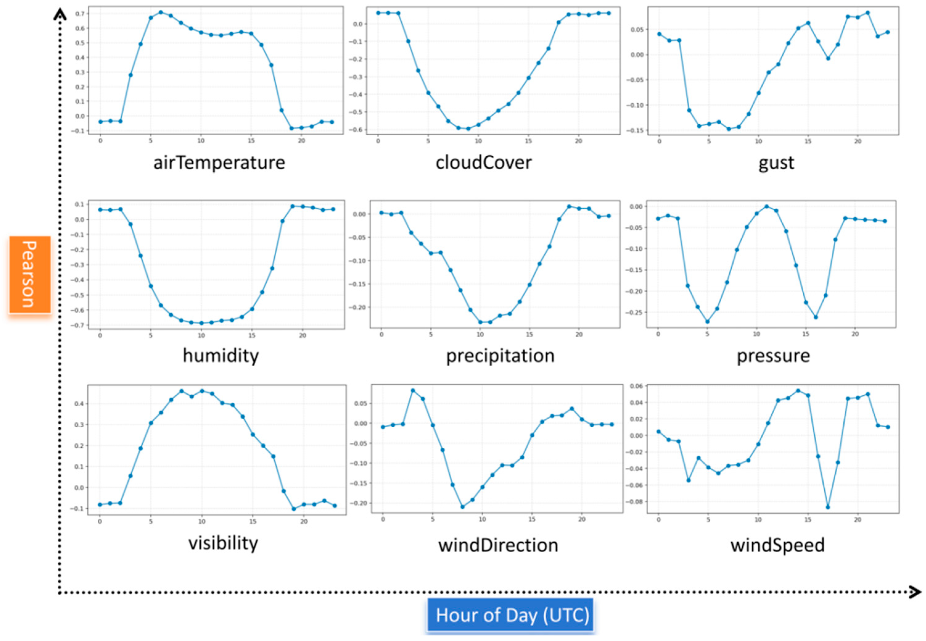
Hourly correlation analysis in Figure 4 reveals a clear diurnal pattern. During daylight hours, air temperature and visibility show strong positive correlations with PV generation, while wind speed and gusts exhibit weaker but still positive effects. In contrast, humidity, cloud cover, and precipitation correlate negatively, with precipitation having a smaller impact. At night, these correlations generally weaken and in some cases reverse. Atmospheric pressure also shows a cyclic trend, with slightly negative values in the early morning and evening, and near-zero or positive values around midday and midnight.

The correlation analysis shows that PV generation correlates strongly and positively with air temperature, and strongly and negatively with humidity, both displaying clear hourly diurnal rhythms. Cloud cover, visibility, and wind speed/gusts exert stronger effects during daylight hours but weaken substantially at night. In addition, synchronous weather systems induce dynamic inter-site correlations. These observations imply that a forecasting model should denoise and extract radiation-related signals, fuse long- and short-term dependencies across multiple temporal scales, and adaptively model time-varying spatial relationships among PV sites. Accordingly, the proposed components—LWS, T-MSFF, and GraphSelfAttention + FSTA—address these core needs, thereby constituting an end-to-end, interpretable, and scalable unified framework.

2.3. Overall Model Architecture

2.3.1. Learnable Wavelet Shrink

Classical wavelet soft-thresholding is effective for time-domain denoising; however, its thresholds are usually set by simple statistical heuristics or empirical rules, remaining hand-crafted and data-independent. By contrast, deep learning models excel at data-driven representation learning, yet often struggle to separate noise from informative high-frequency details when sequences contain substantial noise. To address this, we propose a Learnable Wavelet Shrinkage (LWS) module that preserves the time frequency localization of wavelet decomposition reconstruction while introducing a trainable mechanism that adaptively sets channel-wise shrinkage strength. This enables joint optimization of thresholds with task objectives and data distribution, supporting end-to-end learning of both denoising and feature representation.

Specifically, the input signal is decomposed into an approximation component and a detail component. A lightweight neural network automatically computes channel-wise thresholds from summary statistics of the detail coefficients. The MLP outputs positive thresholds, which are applied via soft-thresholding—that is, coefficients above the threshold are reduced by that amount, whereas coefficients below the threshold are set to zero. Finally, the denoised signal is reconstructed by applying the inverse discrete wavelet transform (IDWT) to the approximation coefficients and the processed detail coefficients.

$${\tilde{D}}_c\left[k\right]=\mathrm{s}\mathrm{i}\mathrm{g}\mathrm{n}\left(D_c\left[k\right]\right)\cdot \mathrm{m}\mathrm{a}\mathrm{x}\left(\left|D_c\left[k\right]\right|-\mathrm{M}\mathrm{L}\mathrm{P}\left(\mathrm{s}\mathrm{t}\mathrm{a}\mathrm{t}\mathrm{s}\left(\left|D_c\right|\right)\right),0\right)$$

(1)

$${\widehat{x}}_c={\mathcal{W}}^{-1}\left(A_c,{\tilde{D}}_c\right)$$

(2)

2.3.2. Temporal Multi-Scale Fine Fusion

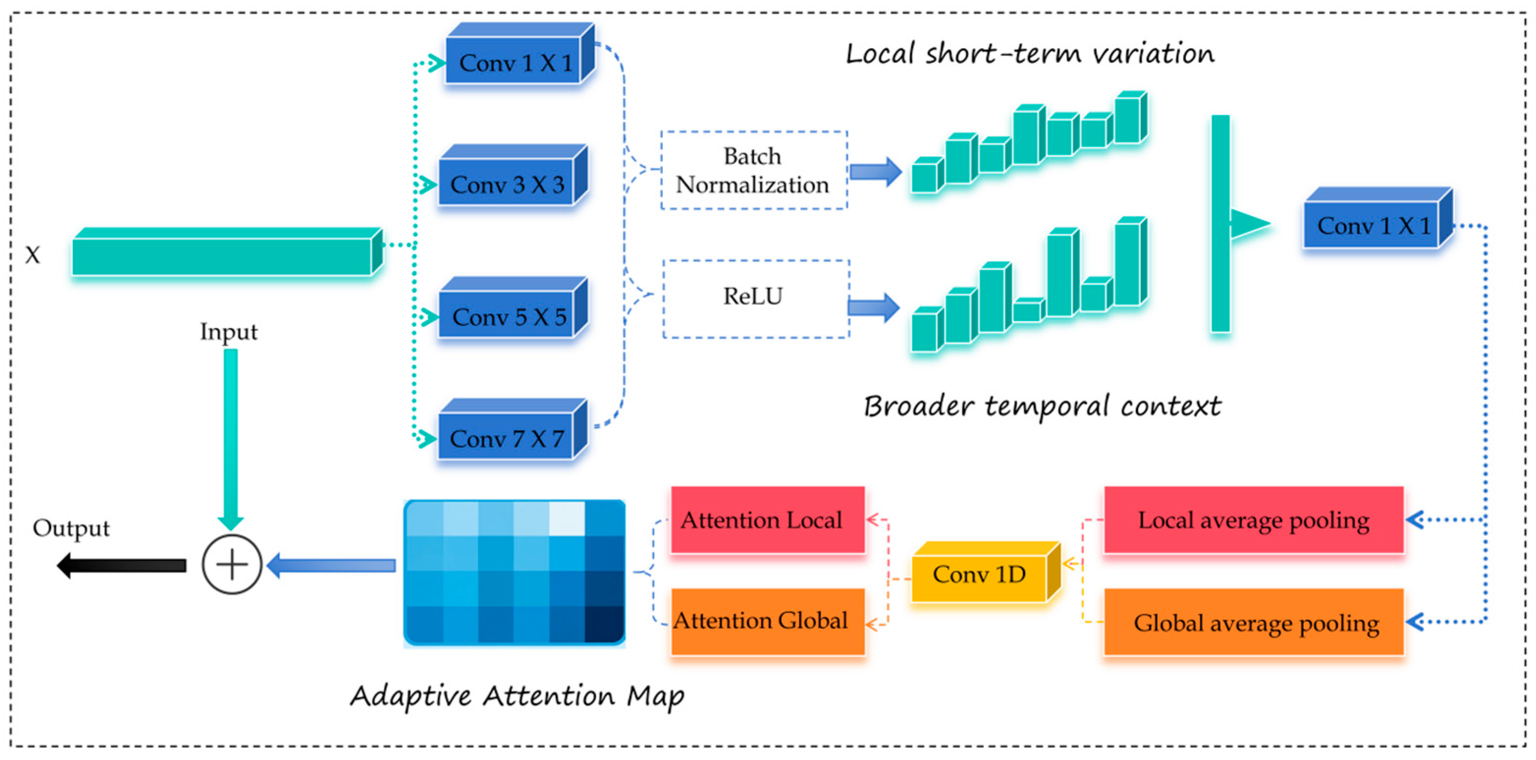
In addition, we introduce a lightweight composite module for one-dimensional signals called Temporal Multi-Scale Fine-Grained Fusion (T-MSFF), as shown in Figure 5. The module employs parallel 1D convolutional branches with different kernel sizes (for example, 3, 5, and 7) to capture temporal patterns over multiple receptive fields. The extracted multi-scale features are then integrated using a 1 × 1 convolution, followed by a residual connection to enhance training stability and maintain information flow. For the attention mechanism, the module first performs local adaptive average pooling to obtain localized temporal summaries, which are subsequently aggregated into channel-level global representations. These channel features are concatenated with local positional embeddings, and a lightweight 1D convolution is applied to the combined sequence to explicitly model interactions between channels and local positions. This process yields a fine-grained channel–position attention map that enables precise feature recalibration.

Furthermore, we incorporate a channel-aware dynamic kernel-size strategy together with a weighted fusion of local and global attention. This design maintains low computational and parameter overhead while jointly capturing local detail and global semantics. Consequently, T-MSFF markedly improves expressive power and attention recalibration across temporal scales, enabling robust noise handling and accurate modeling of short- and long-term dependencies in one-dimensional signal tasks.

2.3.3. Attention Fusion

In sequence modeling, different architectures capture complementary temporal features: LSTM excels at long-term dependencies and sequential dynamics, whereas TCN is well suited to local pattern learning and highly parallel, efficient computation. While naïve concatenation or element-wise addition is possible, these operations cannot adaptively balance the two models’ contributions across samples or feature dimensions. Attention Fusion introduces a parameterized, differentiable mechanism that automatically learns the fusion strategy, enabling end-to-end joint optimization of fusion weights with task objectives.

$$w_1\cdot \mathrm{L}\mathrm{S}\mathrm{T}\mathrm{M}+w_2\cdot \mathrm{T}\mathrm{C}\mathrm{N}$$

(3)

2.3.4. Graph Self-Attention

Classical Graph Neural Networks (GNNs) limit message passing to a fixed adjacency matrix, enabling primarily local information flow. In contrast, Transformer-based self-attention enables global, data-driven interactions but lacks the ability to explicitly incorporate prior geometric or topological structure. Many real-world systems, including multi-site sensor, social, and transportation networks, offer reliable prior adjacencies, but task-specific dependencies beyond these structures still need to be learned.

$$Q=H{W}_Q, K=H{W}_K, V=H{W}_V$$

(4)

$$\tilde{A}=\sigma \left({\displaystyle \frac{A_{\mathrm{p}\mathrm{a}\mathrm{r}\mathrm{a}\mathrm{m}}+A_{\mathrm{p}\mathrm{a}\mathrm{r}\mathrm{a}\mathrm{m}}^{\mathrm{\top }}}{2}}\right)$$

(5)

$$\Lambda ={\displaystyle \frac{Q{K}^{\mathrm{\top }}}{\sqrt{d_k}}}+\alpha \cdot \mathrm{l}\mathrm{o}\mathrm{g}\left(\tilde{A}+\epsilon \right)+\beta \cdot G\left(A_{\mathrm{p}\mathrm{r}\mathrm{i}\mathrm{o}\mathrm{r}}\right)$$

(6)

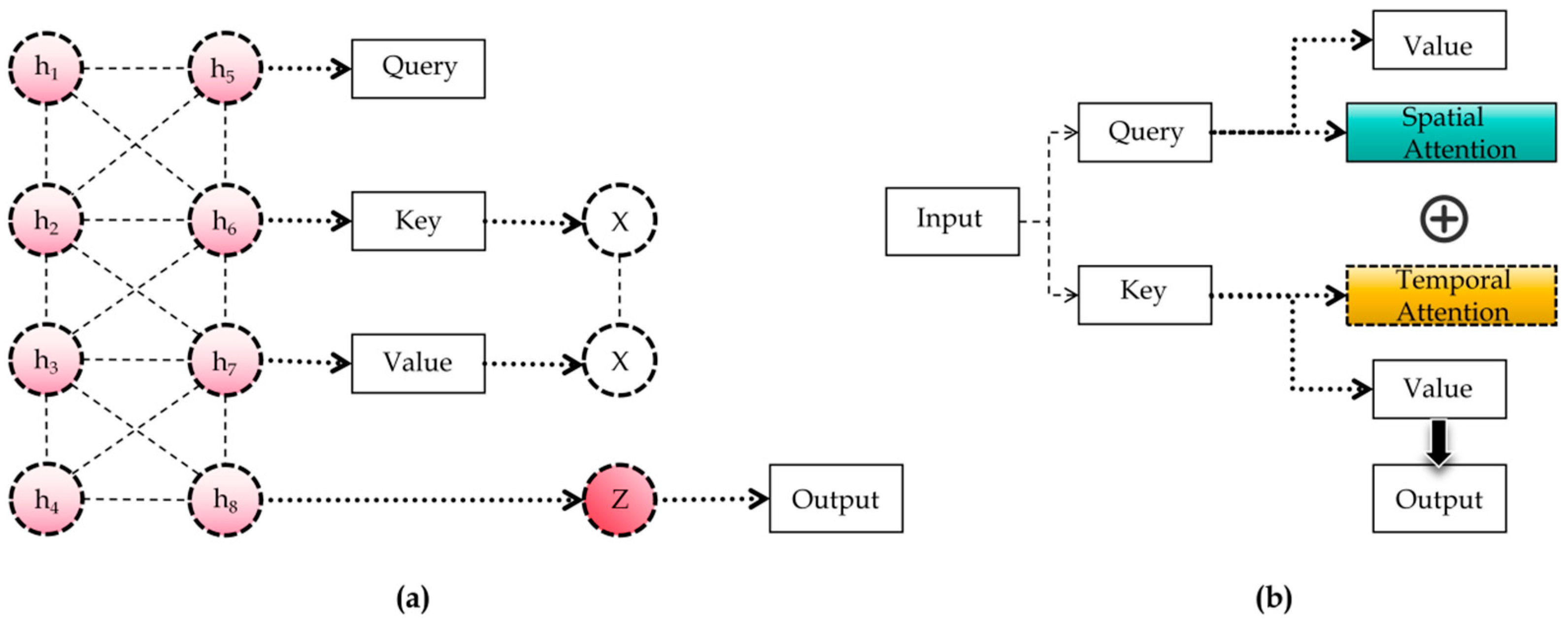
To address this, the Graph Self-Attention (GSA) mechanism introduces optional prior adjacency information into the self-attention logits as either additive or multiplicative biases, while simultaneously learning a trainable adaptive adjacency matrix. This design enables the joint end-to-end learning of both graph structure and interaction weights, as illustrated in Figure 6a.

2.3.5. Factorized Spatio-Temporal Attention

In conventional self-attention mechanisms for spatio-temporal data, each “node–time” pair can be directly treated as a token, upon which global self-attention is applied. While this approach offers strong expressive power, the joint complexity across spatial and temporal dimensions becomes computationally prohibitive when the number of nodes or time steps increases. Conversely, processing temporal modeling (e.g., via LSTM or TCN) and graph modeling (e.g., via GNN) separately fails to flexibly capture fine-grained cross-node and cross-time interactions.

To address these limitations, this study introduces the Factorized Spatio-Temporal Attention (FSTA) module for efficient and interpretable modeling of data characterized by joint node and temporal structures (as shown in Figure 6b). Instead of applying full spatio-temporal attention, which would require computationally intensive joint attention across all nodes and time steps, FSTA decomposes the process into two sequential components: temporal attention followed by spatial (node) attention. This factorization maintains expressive modeling capacity while substantially improving computational and memory efficiency.

Concretely, after linearly projecting the input tensor into the model dimension, multi-head self-attention is first applied along the temporal axis for each node independently, followed by temporal pooling to obtain node-level temporal representations H. Next, multi-head self-attention is performed across nodes on these representations, incorporating a log-bias adjacency matrix that combines learnable adaptive adjacency with prior structural information (scaled and weighted accordingly), yielding spatially enhanced embeddings Z. Finally, Z is aggregated over both nodes and time (e.g., via global average pooling) to obtain a graph-level representation G, which is then passed through Layer Normalization and a lightweight MLP to produce the final prediction output.

$$H_{b,n,:}={\mathrm{P}\mathrm{o}\mathrm{o}\mathrm{l}}_l\left(\mathrm{s}\mathrm{o}\mathrm{f}\mathrm{t}\mathrm{m}\mathrm{a}\mathrm{x}\left({\displaystyle \frac{Q_{b,n}{K}_{b,n}^{\mathrm{\top }}}{\sqrt{d_k}}}\right)V_{b,n}\right)$$

(7)

$$Z_{b,:;:}=\mathrm{s}\mathrm{o}\mathrm{f}\mathrm{t}\mathrm{m}\mathrm{a}\mathrm{x}\left({\displaystyle \frac{Q^{\left(s\right)}{\left(K^{\left(s\right)}\right)}^{\mathrm{\top }}}{\sqrt{d_k}}}+\alpha \cdot \mathrm{l}\mathrm{o}\mathrm{g}\left(\mathrm{c}\mathrm{l}\mathrm{i}\mathrm{p}\left(A_{\mathrm{m}\mathrm{i}\mathrm{x}},\epsilon ,1\right)\right)\right)V^{\left(s\right)}$$

(8)

$$G_b={\displaystyle \frac{1}{L}}\sum _{l=1}^L{\displaystyle \frac{1}{N}}\sum _{n=1}^N{Z}_{b,n,l,:}$$

(9)

$${\widehat{y}}_b=\mathrm{M}\mathrm{L}\mathrm{P}\left(\mathrm{L}\mathrm{a}\mathrm{y}\mathrm{e}\mathrm{r}\mathrm{N}\mathrm{o}\mathrm{r}\mathrm{m}\left(G_b\right)\right)$$

(10)

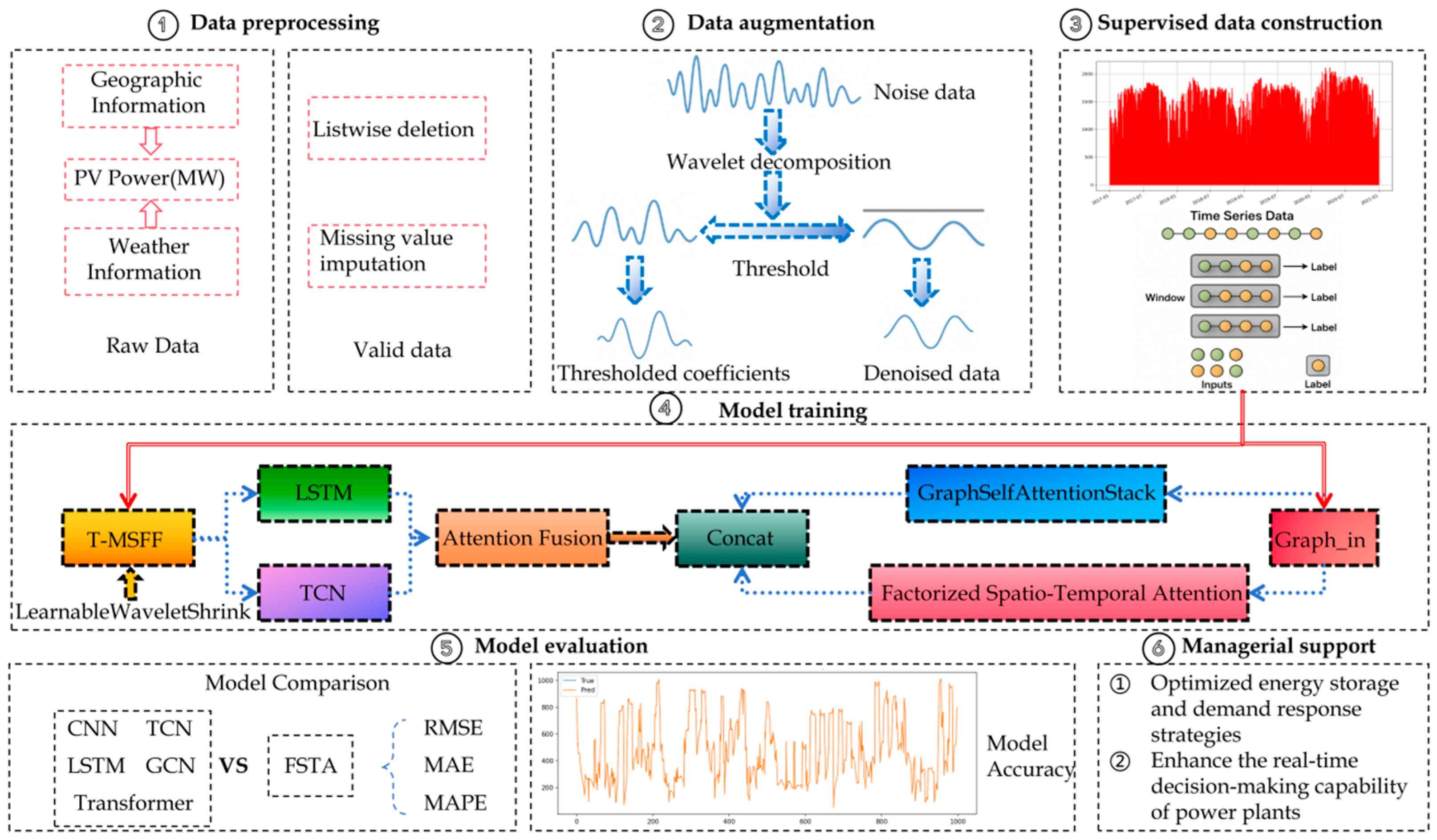
2.4. Overall Framework for Photovoltaic Power Forecasting

The overall framework is shown in Figure 7. First, raw data—including site geolocation, historical power output, and meteorological features—are cleaned via missing-value imputation or listwise deletion. We then perform multi-scale denoising and augmentation using wavelet decomposition with learnable shrinkage. Subsequently, we construct supervised samples with a sliding-window scheme and normalize all features to facilitate training. The model adopts a parallel, multi-branch architecture to balance complementary representational strengths. On one branch, the Temporal Multi-Scale Fine-Grained Fusion (T-MSFF) module processes the wavelet-denoised signal to capture long-term trends and multi-scale temporal components. In the central branch, LSTM and TCN operate in parallel to exploit their respective strengths—long-term dependency modeling and local multi-scale feature extraction. Their outputs are adaptively weighted and fused via an attention-fusion mechanism, then concatenated.

On the other side, graph-based inputs representing site topology are processed using a Graph Self-Attention Stack to model spatial correlations. To efficiently characterize spatio-temporal interactions, a Factorized Spatio-Temporal Attention (FSTA) mechanism is designed, which factorizes temporal and spatial attentions to significantly reduce computational complexity while preserving cross-time and cross-node information exchange.

Finally, the model outputs the PV power forecasts, and performance is evaluated using standard metrics such as RMSE, MAE, and MAPE. This framework achieves enhanced prediction accuracy and robustness through the fusion of multimodal, multi-scale, and spatio-graph structures, and can be directly applied to support energy storage scheduling optimization and real-time decision enhancement in photovoltaic power plants.

3. Experimental Setup and Results Analysis

In this section, we evaluate the proposed WGL method on a multi-site dataset across multiple forecasting horizons and training scales. All experiments were conducted on Windows using the PyCharm development environment. Hardware consisted of an Intel Core i7-14700KF (3.40 GHz), 16 GB RAM, and an NVIDIA GeForce RTX 4090D (24 GB VRAM). The software stack included Python 3.10, CUDA 12.1, and PyTorch 2.0.1 (cu12.1). Detailed experimental parameters are summarized in

Table 3. Detailed parameters of the example segmentation model.

Parameters
seed	42
train_ratio	0.8
lr	0.001
epoch	50
batch	16
workers	0
optimizer	Adam
forecast_horizon	1/2/3
num_time_steps	6/12

.

3.1. Evaluation Metrics

For a comprehensive assessment of WGL, we adopt three standard metrics: mean absolute error (MAE), root mean square error (RMSE), and mean absolute percentage error (MAPE). The corresponding formulas are as follows:

$$\mathrm{M}\mathrm{A}\mathrm{E}={\displaystyle \frac{1}{n}}\sum _{i=1}^n\left|y_i-{\widehat{y}}_i\right|$$

(11)

$$\mathrm{R}\mathrm{M}\mathrm{S}\mathrm{E}=\sqrt{{\displaystyle \frac{1}{n}}\sum _{i=1}^n{\left(y_i-{\widehat{y}}_i\right)}^2}$$

(12)

$$\mathrm{M}\mathrm{A}\mathrm{P}\mathrm{E}={\displaystyle \frac{100\mathrm{\%}}{n}}\sum _{i=1}^n\left|{\displaystyle \frac{y_i-{\widehat{y}}_i}{y_i}}\right|$$

(13)

For clarity, when highlighting WGL’s advantages, RMSE, MAE, and MAPE are each scaled by 1/100, aligning their magnitudes and making comparisons more transparent. Directionality remains intact under this normalization (smaller is better), and neither relative rankings nor statistical inferences are affected.

3.2. Experimental Results and Comparative Analysis

In this study, the TCN–LSTM architecture is designated as the baseline, and a comprehensive suite of modular ablation experiments is orchestrated within the proposed WGL framework, enabling a systematic dissection of each component’s functional contribution to the overall predictive efficacy. All experiments are conducted on a three-year corpus of historical PV generation data, employing a 12-h look-back window and a 1-h forecasting horizon to emulate ultra-short-term operational conditions. Through the progressive incorporation of key WGL modules atop the baseline, the study conducts a granular investigation into each component’s role in capturing temporal dependencies and delineating spatial feature interactions.

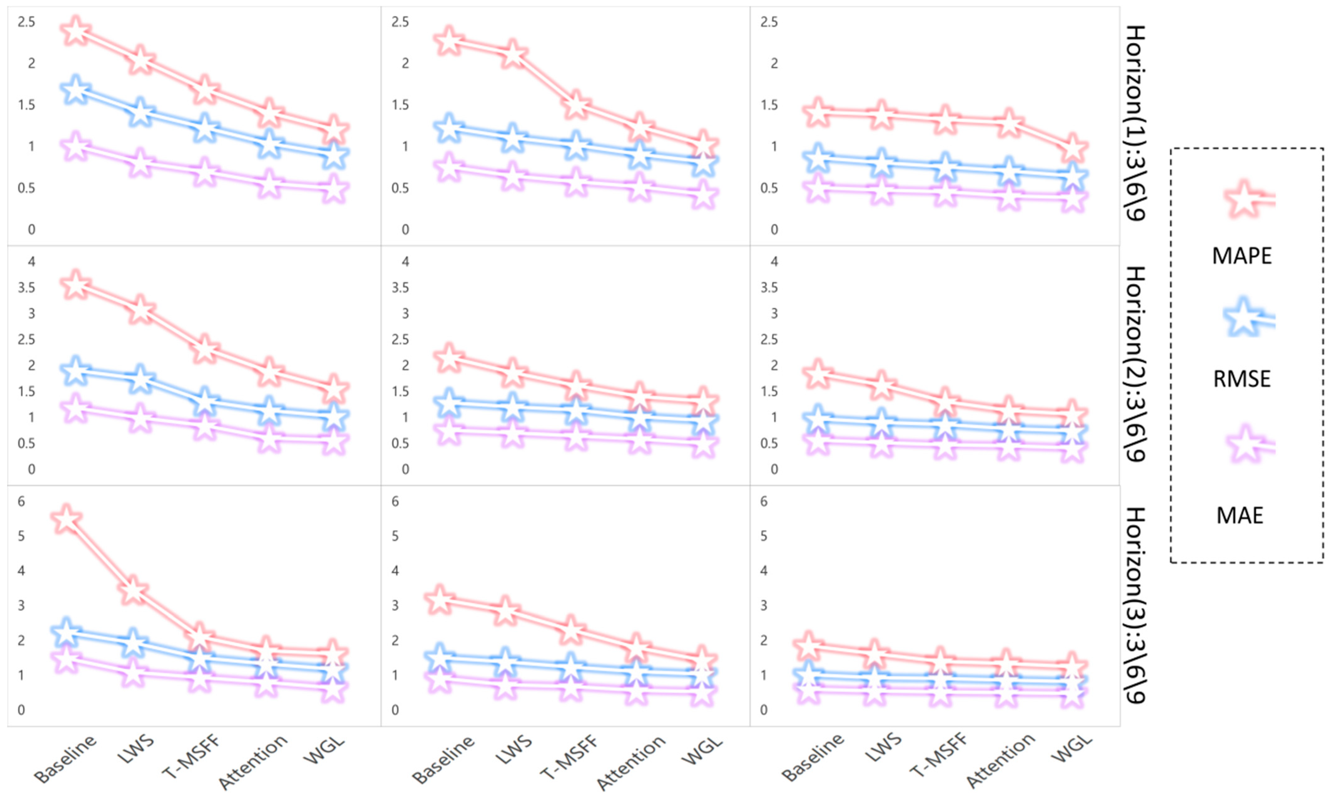
As evidenced by the quantitative results in

Table 4. Ablation experiment results of different module combinations in the 12-step prediction.

Model	Step(12)						RMSE\MAE\MAPE
	Baseline	LWS	T-MSFF	GSA	FSTA	WGL
Baseline	✓						0.80\0.50\1.39
LWS	✓	✓					0.72\0.45\1.31
T-MSFF	✓	✓	✓				0.65\0.41\1.14
GSA	✓	✓	✓	✓			0.62\0.37\1.05
FSTA	✓	✓	✓	✓	✓		0.60\0.36\1.01
WGL	✓	✓	✓	✓	✓	✓	0.57\0.33\0.91

, the ablation experiments conducted at a 1 h forecasting horizon reveal that the baseline model attains an RMSE of 0.80, an MAE of 0.50, and a MAPE of 1.39. Upon incorporating the attention-oriented modules (Attention Fusion, GSA, and FSTA), the error metrics decline to 0.60, 0.36, and 1.01, respectively. Building on these results, the proposed WGL framework achieves further reductions—RMSE = 0.57, MAE = 0.33, MAPE = 0.91—corresponding to relative improvements of 28.8%, 34.0%, and 34.5% over the baseline, and additional decreases of 5.0%, 8.3%, and 9.9% relative to the attention-only configuration. From a mechanistic perspective, LWS performs adaptive denoising via trainable shrinkage embedded in a wavelet decomposition–reconstruction framework, thereby enhancing the robustness of time–frequency-localized features. Attention Fusion introduces a differentiable attention mechanism that adaptively balances the respective contributions of LSTM and TCN across sample and feature dimensions, effectively integrating long-term dependencies with local temporal patterns. GSA integrates prior adjacency as a bias term while jointly learning an adaptive adjacency matrix, achieving a synergistic balance between geometric priors and task-specific relations. Finally, FSTA factorizes comprehensive spatio-temporal attention into temporal and node-level subspaces, markedly reducing computational and memory complexity while maintaining fine-grained cross-time and cross-node interactions. Overall, the WGL framework coherently integrates denoising and recalibration (LWS), adaptive fusion (Attention Fusion), and structure-aware spatio-temporal attention (GSA + FSTA) within a unified architecture, thereby mitigating systematic bias, suppressing extreme residuals, and delivering stable and cumulative performance gains.

As illustrated by the comparative analyses presented in Figure 8, three evaluation metrics—MAPE, RMSE, and MAE—are employed to rigorously assess the performance of five representative models (Baseline, LWS, T-MSFF, Attention, and WGL) across three experimental scenarios and forecasting horizons of 3, 6, and 9 h. The results reveal a consistent decline in prediction errors as model complexity increases, with WGL attaining the lowest MAPE, RMSE, and MAE across all scenarios and horizons, thereby demonstrating its comprehensive performance advantage. Notably, under more challenging conditions—characterized by higher baseline errors and extended forecasting horizons—WGL achieves markedly greater error reductions, indicating that the proposed framework not only enhances point-estimate accuracy but also effectively mitigates extreme deviations and noise perturbations.

For benchmarking purposes, the proposed WGL framework is evaluated against several representative deep learning architectures, including GCN, CNN, LSTM, TCN, Transformer [29], CNN–LSTM [30], and Transformer–LSTM [31]. All comparative experiments are trained on a three-year corpus of historical PV generation data, employing a 12-h look-back window as input and forecasting targets of 1, 2, and 3 h ahead.

As evidenced by the quantitative results presented in

Table 5. Performance comparison of different models under 12-step prediction across various prediction horizons.

Model	RMSE\MAE\MAPE\Step(12)
	Horizon(1)	Horizon(2)	Horizon(3)
GCN	3.16\2.06\6.40	3.25\2.21\7.58	3.31\2.27\8.09
CNN	1.87\1.18\4.17	2.05\1.35\6.69	2.29\1.43\6.68
LSTM	1.21\0.73\2.65	1.31\0.80\2.67	1.48\0.88\3.35
TCN	1.47\0.85\2.33	1.63\0.96\3.34	1.68\0.97\3.32
Transformer	1.71\0.99\2.85	2.00\1.24\5.04	2.01\1.30\5.89
CNN-LSTM	0.74\0.49\1.29	0.85\0.58\1.41	0.97\0.60\1.69
Transformer-LSTM	1.69\1.01\3.34	1.80\1.06\4.09	2.01\1.23\6.34
WGL	0.57\0.33\0.91	0.62\0.37\1.03	0.65\0.39\1.21

, under an identical input sequence length of 12 h, the proposed WGL model consistently delivers superior predictive performance across all forecasting horizons. At a forecasting horizon of 3 h, WGL attains RMSE = 0.65, MAE = 0.39, and MAPE = 1.21, corresponding to reductions of approximately 33%, 35%, and 28% relative to CNN–LSTM (0.97/0.60/1.69). Furthermore, when compared with single-architecture baselines such as LSTM, TCN, and Transformer (e.g., for a 1 h horizon: LSTM = 1.21/0.73/2.65; TCN = 1.47/0.85/2.33), WGL exhibits even more pronounced advantages. Collectively, these results demonstrate that under a unified input configuration, WGL consistently yields lower forecasting errors across all short-term horizons, underscoring its enhanced capacity to capture complex temporal dependencies and nonlinear dynamics, while maintaining robust stability and strong generalization in hour-level photovoltaic power forecasting.

The results in

Table 6. Comparison of model complexity and inference performance.

	Params	MFLOPs	Latency
CNN	8.129K	0.086	15.91
CNN-LSTM	372.77K	6.61	14.19
LSTM	24.19K	0.126	11.16
TCN	139.17K	2.204	10.11
Transformer	415.75K	7.275	9.56
Transformer-LSTM	415.4K	6	9.91
WGL	325K	5.12	6.15

show significant differences among the models in terms of parameter count, computational cost, and latency. Although CNN is the lightest model, it has the highest latency, indicating lower parallel efficiency. TCN and LSTM achieve reduced latency, while CNN-LSTM maintains a reasonable delay despite increased computation. The Transformer-based models exhibit relatively low latency even with larger parameter sizes, demonstrating strong parallel performance. Overall, WGL performs best with the lowest latency (6.15), suggesting a more efficient architectural design.

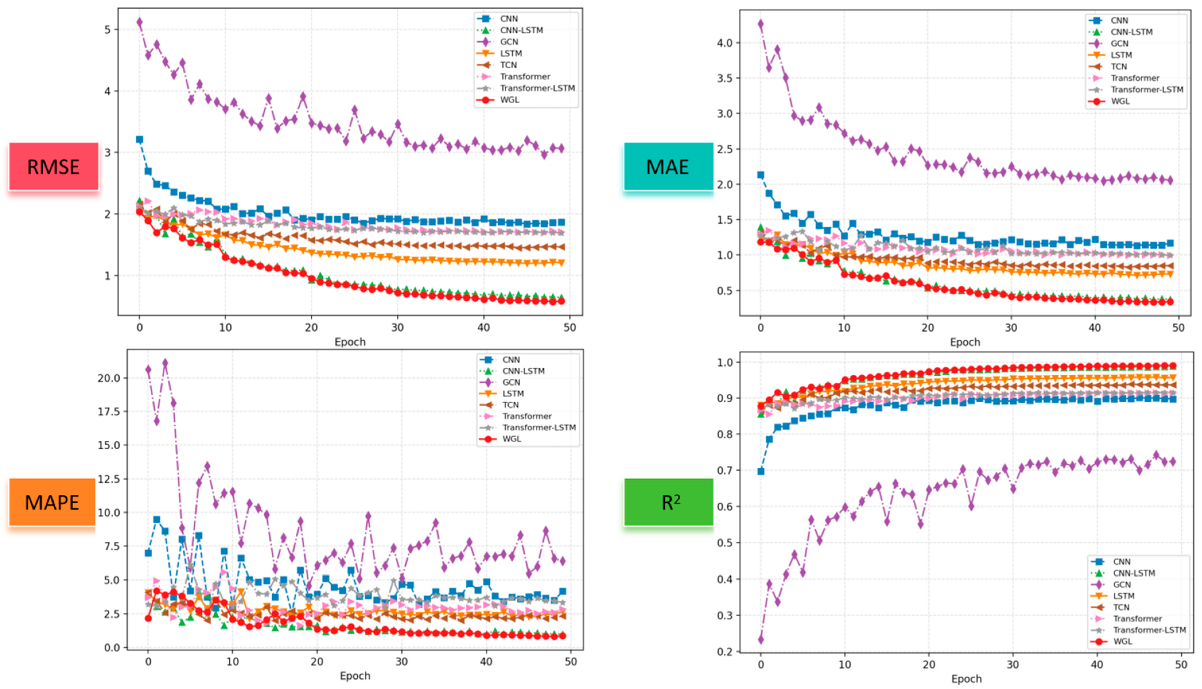
Figure 9 presents four subplots illustrating the evolution of RMSE, MAE, MAPE, and R² across training epochs for different models. Most models begin with comparatively high initial errors that progressively decline and eventually stabilize; nevertheless, their convergence rates, terminal error magnitudes, and training stability differ substantially. In particular, the WGL model (red curve) consistently surpasses all counterparts across every evaluation metric, exhibiting the fastest convergence, the smoothest training trajectory (with minimal oscillations), the lowest terminal RMSE, MAE, and MAPE, and the highest and most stable R² values. By contrast, several alternative models exhibit noticeable oscillations during early-stage training and slower convergence, with certain architectures showing pronounced MAPE fluctuations—an indication of heightened sensitivity to outliers and limited-sample variability.

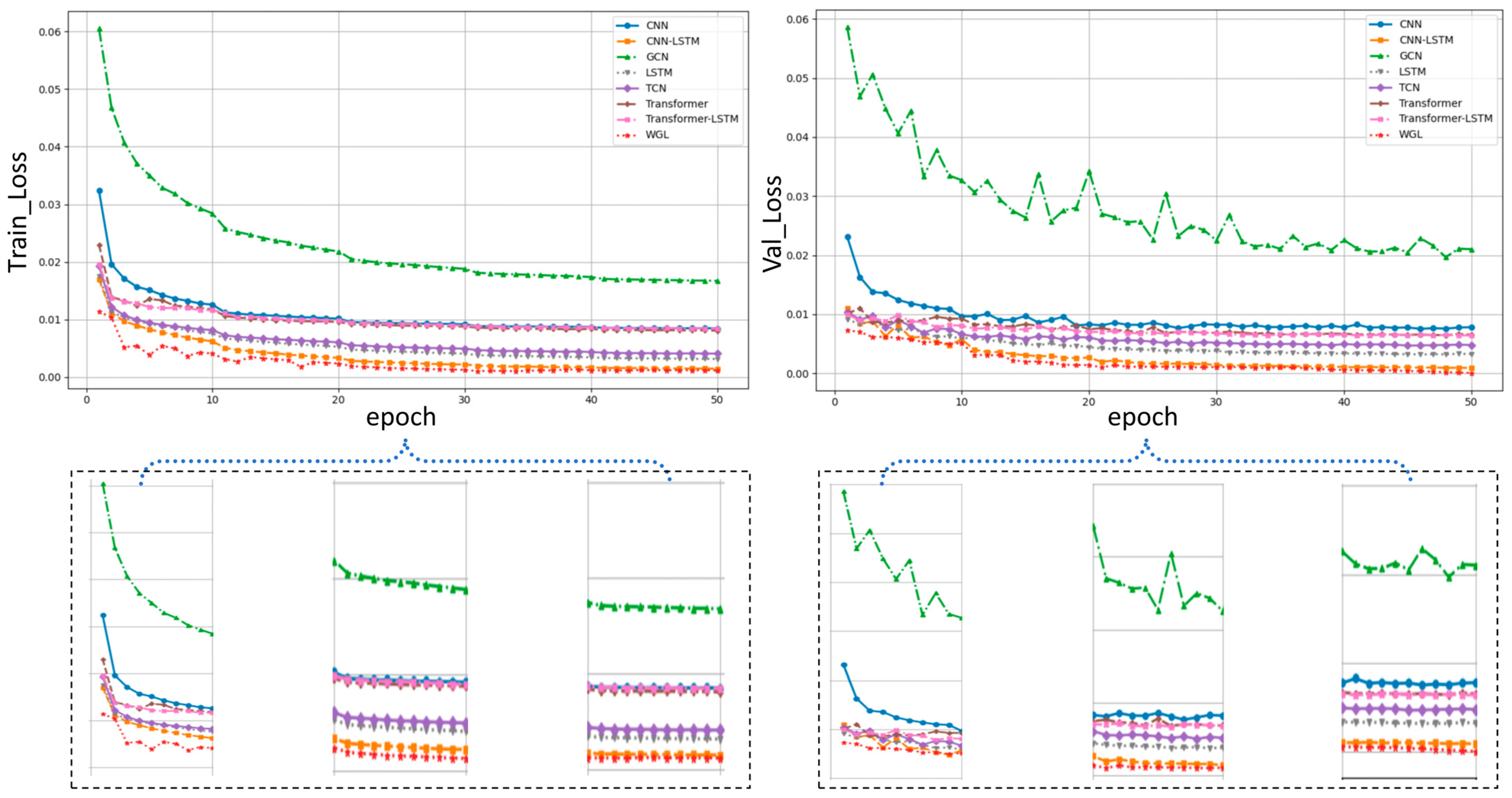
The convergence behavior illustrated in Figure 10 highlights that the proposed WGL model consistently outperforms all comparative baselines—including CNN, LSTM, TCN, Transformer, and their hybrid variants—in convergence speed, loss attenuation, and training–validation coherence. The WGL model rapidly converges toward a low-loss regime during the initial training phase and remains exceptionally stable thereafter, ultimately attaining the lowest and most consistent validation loss among all evaluated models. Collectively, these observations confirm that WGL exhibits superior representational capacity, strong generalization, and marked resilience to noise perturbations.

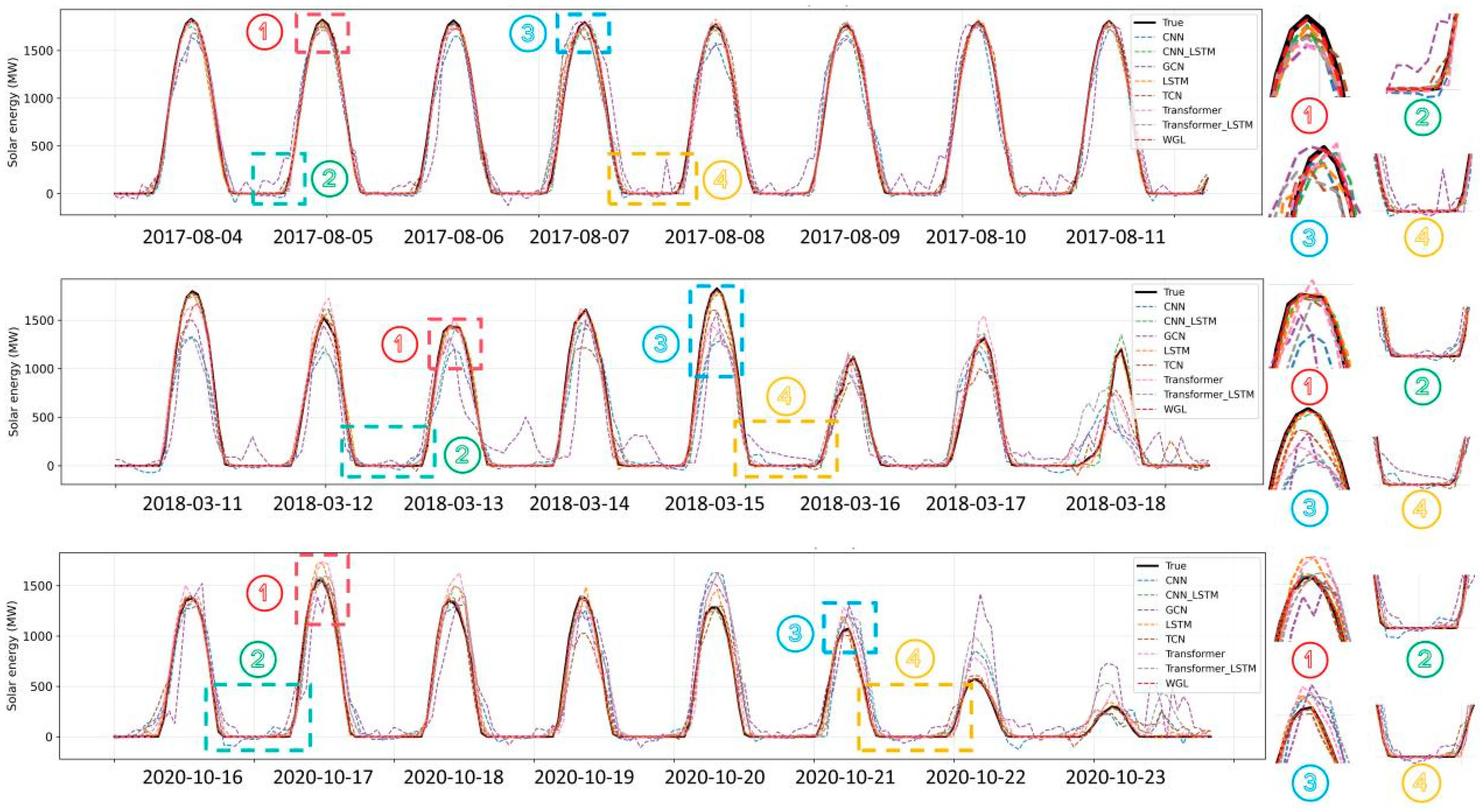
An inspection of Figure 11 reveals that the proposed WGL model more faithfully reproduces the true intraday photovoltaic power trajectories across diverse dates and meteorological conditions. In particular, WGL effectively mitigates overshooting and peak clipping around midday, precisely reconstructing peak amplitudes; it exhibits reduced phase lag during the steep ascent and descent transitions at dawn and dusk; it promptly responds to short-term irradiance-induced power dips while preserving their morphological integrity without over-smoothing; and it sustains a stable baseline throughout low-power tail segments with negligible deviation. These empirical observations suggest that WGL achieves an optimal balance between capturing local transient dynamics and preserving the overarching diurnal periodic structure. Relative to conventional baselines—including CNN, RNN, TCN, and Transformer—the WGL framework yields markedly lower systematic errors and enhanced robustness with respect to amplitude deviation, phase lag, and transient responsiveness, thereby underscoring its superior short-term predictive accuracy and cross-scenario generalization.

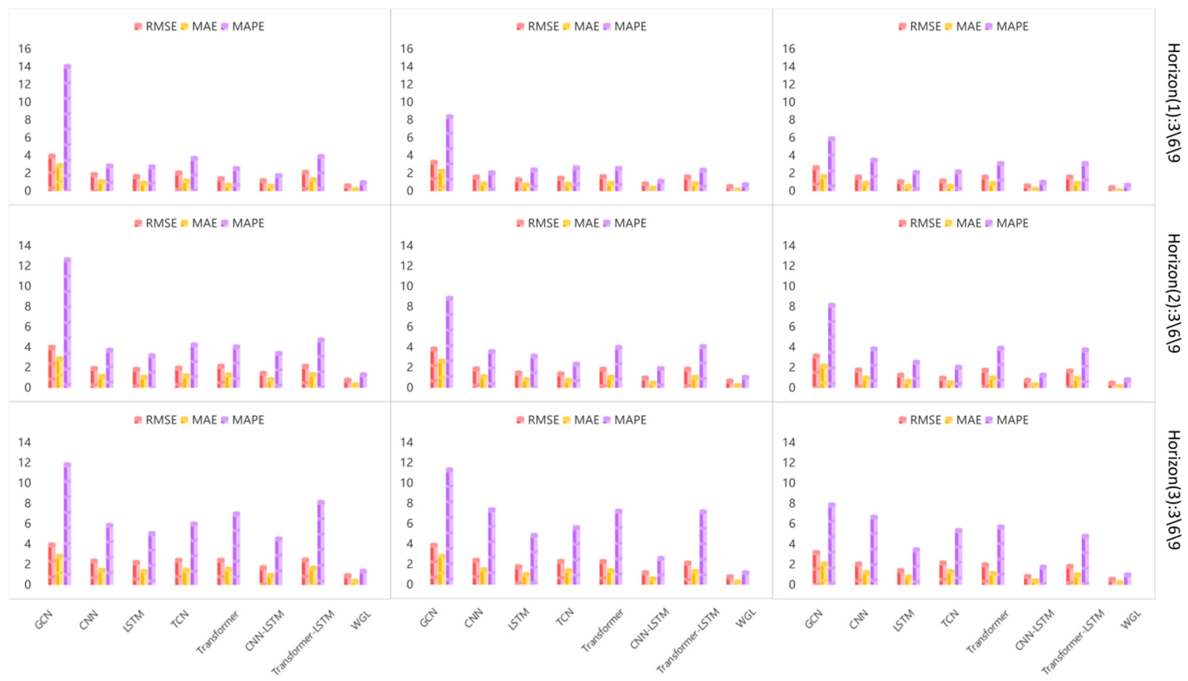
Figure 12 presents comparative results indicating that the proposed WGL framework substantially surpasses all competing baselines across multiple evaluation criteria—namely RMSE, MAE, and MAPE—under various forecasting horizons. WGL not only attains the lowest absolute errors in terms of RMSE and MAE but also delivers distinctly superior performance in relative error (MAPE). Furthermore, as the forecasting horizon extends, WGL exhibits a markedly slower increase in error magnitude, reflecting its enhanced stability and robustness across short-, medium-, and long-term forecasting horizons.

From

Table 7. Comparison of Prediction Performance Based on 18 Wind Farms.

Model	RMSE\MAE\MAPE\Horizon(1)
	STEPS(3)	STEPS(6)	STEPS(9)	STEPS(12)
GCN	5.41\4.09\1.21	3.92\3.03\1.05	3.58\2.76\0.94	3.47\2.68\0.88
CNN	3.70\2.90\1.05	3.65\2.86\1.03	3.61\2.85\1.05	3.52\2.71\0.99
LSTM	3.36\2.56\0.90	3.33\2.53\0.87	3.29\2.49\0.83	3.18\2.37\0.80
TCN	5.49\4.24\1.58	4.05\3.21\1.23	3.68\3.01\1.06	3.22\2.87\1.01
Transformer	5.28\3.92\1.15	5.11\3.81\1.10	4.92\3.65\0.96	4.71\3.51\0.93
CNN-LSTM	2.71\1.87\0.91	2.60\1.75\0.85	2.53\1.71\0.80	2.50\1.68\0.78
Transformer-LSTM	5.21\3.86\1.11	5.09\3.76\1.02	4.87\3.61\0.94	4.65\3.46\0.87
WGL	1.65\1.21\0.65	1.52\1.10\0.60	1.38\0.92\0.51	1.21\0.83\0.47

, it can be observed that the overall errors of most models decrease as the input length increases, indicating that a longer historical window contributes positively to short-term forecasting performance. Among the baseline models, CNN-LSTM consistently outperforms single-architecture models such as LSTM, TCN, and Transformer, while GCN exhibits the weakest performance in this task. Compared with all baselines, WGL achieves the best results across all four input lengths and all three evaluation metrics, with its relative advantage becoming more pronounced at longer input lengths. Specifically, compared with the strong baseline CNN-LSTM, WGL reduces RMSE, MAE, and MAPE by up to approximately 46%, 51%, and 40%, respectively. These results demonstrate that WGL can more effectively leverage long-term temporal information and model key patterns that affect one-step forecasting accuracy.

4. Discussion

Building on prior experimental results, the proposed spatio-temporal graph-based deep learning framework (WGL) shows strong potential for PV power forecasting. Moving toward real-world deployment requires coordination across four areas: cost, safety, governance, and user-centered design. The plan uses cloud–edge collaboration to shift upfront costs into flexible operations, with validation through small, seasonal and climatic pilot tests. It includes safeguards such as encrypted data, access control, model fallback, system protection, and standard maintenance to ensure safety. It also aligns roles, procedures, and MLOps workflows. Finally, it embeds interpretability and uncertainty into alerts to support clear and accountable decisions.

Ensuring generalizability and adaptability across regions and climates requires evaluating target-domain data availability, identifying distribution shifts, developing unified temporal and metadata pipelines, applying localized preprocessing and quality control, and adopting hierarchical transfer strategies such as few-shot tuning, domain adaptation, multi-domain training, or meta-learning, along with calibrated confidence estimation. Cross-climate pilot studies in representative climate zones should be conducted to validate model generalization and economic value, with clear KPIs defined for accuracy, probabilistic calibration, and cost-effectiveness. Online deployment should incorporate concept drift detection and automated fallback, following a pilot-first, post-validation scaling path to transition WGL from a research prototype into a robust and replicable system deployable across diverse environments.

5. Conclusions

In this work, we advance Wavelet–Graph Learning (WGL), an end-to-end and unified modeling paradigm designed for intra-hour, multi-step forecasting of multi-site photovoltaic (PV) power generation. The framework integrates learnable wavelet shrinkage for adaptive noise suppression, a Temporal Multi-Scale Fine-Grained Fusion (T-MSFF) mechanism for extracting complementary temporal representations, and an attention-fusion gate for the dynamic integration of TCN and LSTM architectures. Along the spatial dimension, Graph Self-Attention (GSA) captures latent inter-station dependencies, while Factorized Spatio-Temporal Attention (FSTA) efficiently models long-range, cross-site interactions.

Empirical evaluations demonstrate that WGL consistently and substantially outperforms strong baselines across multiple forecasting horizons, while ablation analyses validate the complementary effects and synergistic contributions of its constituent modules, underscoring both its predictive accuracy and deployment potential. From an engineering standpoint, WGL consolidates denoising, multi-scale fusion, and graph-based spatio-temporal modeling within a unified architecture, thereby minimizing reliance on handcrafted feature engineering and rule-based post-processing. Under constrained computational complexity, it enhances cross-site information integration and effectively represents both short- and long-term dependencies, yielding robust short-term forecasts for practical grid dispatch and storage management.

Beyond algorithmic performance, a systematic assessment was undertaken to examine the framework’s deployment feasibility from the perspectives of safety, economic viability, managerial governance, and human-centered design. This comprehensive evaluation underscores that the successful deployment of WGL depends not only on predictive accuracy but equally on addressing key challenges in data security, model reliability, economic sustainability, organizational integration, and stakeholder trust.

Despite the encouraging results, several aspects warrant further refinement. The current dataset encompasses a limited range of sites and climatic zones; the marginal contributions of the attention submodules merit deeper disentanglement; efficiency indicators—including inference latency, parameter complexity, and energy consumption—require more systematic benchmarking; and the model’s robustness to missing data, distributional shifts, and uncertainty quantification remains to be reinforced. Moreover, the implementation analysis underscores the importance of future research in rigorously addressing cybersecurity vulnerabilities, formulating cost-efficient deployment strategies for large-scale grid environments, and instituting standardized MLOps frameworks for reliable lifecycle management.

References

1. Iheanetu, K.J. Solar photovoltaic power forecasting: A review. Sustainability 2022, 14, 17005. [Google Scholar] [CrossRef]
2. Gupta, P.; Singh, R. PV power forecasting based on data-driven models: A review. Int. J. Sustain. Eng. 2021, 14, 1733–1755. [Google Scholar] [CrossRef]
3. Chodakowska, E.; Nazarko, J.; Nazarko, Ł.; Rabayah, H.S.; Abendeh, R.M.; Alawneh, R. ARIMA models in solar radiation forecasting in different geographic locations. Energies 2023, 16, 5029. [Google Scholar] [CrossRef]
4. Yang, Y.; Yu, T.; Zhao, W.; Zhu, X. Kalman filter photovoltaic power prediction model based on forecasting experience. Front. Energy Res. 2021, 9, 682852. [Google Scholar] [CrossRef]
5. Mayer, M.J.; Yang, D.; Szintai, B. Comparing global and regional downscaled NWP models for irradiance and photovoltaic power forecasting: ECMWF versus AROME. Appl. Energy 2023, 352, 121958. [Google Scholar] [CrossRef]
6. Böök, H.; Lindfors, A.V. Site-specific adjustment of a NWP-based photovoltaic production forecast. Sol. Energy 2020, 211, 779–788. [Google Scholar] [CrossRef]
7. He, Y.; Gao, Q.; Jin, Y.; Liu, F. Short-term photovoltaic power forecasting method based on convolutional neural network. Energy Rep. 2022, 8, 54–62. [Google Scholar] [CrossRef]
8. Ahn, H.K.; Park, N. Deep RNN-based photovoltaic power short-term forecast using power IoT sensors. Energies 2021, 14, 436. [Google Scholar] [CrossRef]
9. Konstantinou, M.; Peratikou, S.; Charalambides, A.G. Solar photovoltaic forecasting of power output using LSTM networks. Atmosphere 2021, 12, 124. [Google Scholar] [CrossRef]
10. Li, Y.; Song, L.; Zhang, S.; Kraus, L.; Adcox, T.; Willardson, R.; Komandur, A.; Lu, N. A TCN-based hybrid forecasting framework for hours-ahead utility-scale PV forecasting. IEEE Trans. Smart Grid 2023, 14, 4073–4085. [Google Scholar] [CrossRef]
11. Campos, F.D.; Sousa, T.C.; Barbosa, R.S. Short-term forecast of photovoltaic solar energy production using lstm. Energies 2024, 17, 2582. [Google Scholar] [CrossRef]
12. Chu, Y.; Wang, Y.; Yang, D.; Chen, S.; Li, M. A review of distributed solar forecasting with remote sensing and deep learning. Renew. Sustain. Energy Rev. 2024, 198, 114391. [Google Scholar] [CrossRef]
13. Al Mouloud, L.; Kheldoun, A.; Oussidhoum, S.; Alharbi, H.; Alotaibi, S.; Alzahrani, T.; Agajie, T.F. Seasonal quantile forecasting of solar photovoltaic power using Q-CNN-GRU. Sci. Rep. 2025, 15, 27270. [Google Scholar] [CrossRef]
14. Wang, J.; Li, G.; Gu, J.; Xu, Z.; Chen, X.; Wei, J. Short term prediction of photovoltaic power with time embedding temporal convolutional networks. Sci. Rep. 2025, 15, 22400. [Google Scholar] [CrossRef]
15. Simeunovic, J.; Schubnel, B.; Alet, P.-J.; Carrillo, R.E. Spatio-temporal graph neural networks for multi-site PV power forecasting. IEEE Trans. Sustain. Energy 2021, 13, 1210–1220. [Google Scholar] [CrossRef]
16. Yang, Y.; Liu, Y.; Zhang, Y.; Shu, S.; Zheng, J. DEST-GNN: A double-explored spatio-temporal graph neural network for multi-site intra-hour PV power forecasting. Appl. Energy 2025, 378, 124744. [Google Scholar] [CrossRef]
17. Zhang, M.; Zhen, Z.; Liu, N.; Zhao, H.; Sun, Y.; Feng, C.; Wang, F. Optimal graph structure based short-term solar PV power forecasting method considering surrounding spatio-temporal correlations. IEEE Trans. Ind. Appl. 2022, 59, 345–357. [Google Scholar] [CrossRef]
18. Zang, H.; Zhang, Y.; Cheng, L.; Ding, T.; Wei, Z.; Sun, G. Multi-site solar irradiance forecasting based on adaptive spatiotemporal graph convolutional network. Expert. Syst. Appl. 2024, 236, 121313. [Google Scholar] [CrossRef]
19. Yao, T.; Wang, J.; Wang, Y.; Zhang, P.; Cao, H.; Chi, X.; Shi, M. Very short-term forecasting of distributed PV power using GSTANN. CSEE J. Power Energy Syst. 2022, 10, 1491–1501. [Google Scholar]
20. Fan, T.; Sun, T.; Liu, H.; Xie, X.; Na, Z. Spatial-temporal genetic-based attention networks for short-term photovoltaic power forecasting. IEEE Access 2021, 9, 138762–138774. [Google Scholar] [CrossRef]
21. Zhen, Z.; Yang, Y.; Wang, F.; Yu, N.; Huang, G.; Chang, X.; Li, G. PV power forecasting method using a dynamic spatio-temporal attention graph convolutional network with error correction. Sol. Energy 2025, 300, 113770. [Google Scholar] [CrossRef]
22. Yang, M.; Wang, Z.; Chen, H. Spatiotemporal attention network for ultra-short-term photovoltaic power forecasting considering spatiotemporal correlations and multiple environmental factors. AIMS Energy 2025, 13, 1104–1132. [Google Scholar] [CrossRef]
23. Jing, S.; Xi, X.; Su, D.; Han, Z.; Wang, D. Spatio-Temporal Photovoltaic Power Prediction with Fourier Graph Neural Network. Electronics 2024, 13, 4988. [Google Scholar] [CrossRef]
24. Jin, M.; Koh, H.Y.; Wen, Q.; Zambon, D.; Alippi, C.; Webb, G.I.; King, I.; Pan, S. A survey on graph neural networks for time series: Forecasting, classification, imputation, and anomaly detection. IEEE Trans. Pattern Anal. Mach. Intell. 2024, 46, 10466–10485. [Google Scholar] [CrossRef] [PubMed]
25. Tan, L.; Kang, R.; Xia, J.; Wang, Y. Application of multi-source data fusion on intelligent prediction of photovoltaic power. Sol. Energy 2024, 277, 112706. [Google Scholar] [CrossRef]
26. Yao, T.; Wang, J.; Wu, H.; Zhang, P.; Li, S.; Xu, K.; Liu, X.; Chi, X. Intra-hour photovoltaic generation forecasting based on multi-source data and deep learning methods. IEEE Trans. Sustain. Energy 2021, 13, 607–618. [Google Scholar] [CrossRef]
27. Liu, X.; Liu, Y.; Kong, X.; Ma, L.; Besheer, A.H.; Lee, K.Y. Deep neural network for forecasting of photovoltaic power based on wavelet packet decomposition with similar day analysis. Energy 2023, 271, 126963. [Google Scholar] [CrossRef]
28. Liu, L.; Zhang, J.; Xue, S. Photovoltaic power forecasting: Using wavelet threshold denoising combined with VMD. Renew. Energy 2025, 249, 123152. [Google Scholar] [CrossRef]
29. Piantadosi, G.; Dutto, S.; Galli, A.; De Vito, S.; Sansone, C.; Di Francia, G. Photovoltaic power forecasting: A Transformer based framework. Energy AI 2024, 18, 100444. [Google Scholar] [CrossRef]
30. Wang, K.; Qi, X.; Liu, H. Photovoltaic power forecasting based LSTM-Convolutional Network. Energy 2019, 189, 116225. [Google Scholar] [CrossRef]
31. Zhang, R.; Wan, X.; Bu, S.; Zhou, M.; Zeng, Q.; Zhang, Z. Interpretable prediction of multi-photovoltaic power stations via spatial-temporal multi-task learning with Transformer-XLSTM. Results Eng. 2025, 28, 107369. [Google Scholar] [CrossRef]
Figure 1. Problem definition structure.
Electronics 14 04492 g001
Figure 2. Distribution plot of Pearson correlation coefficients.
Electronics 14 04492 g002
Figure 3. Heatmap of correlation analysis among factors.
Electronics 14 04492 g003
Figure 4. Diurnal variation of Pearson correlations between meteorological variables and photovoltaic power.
Electronics 14 04492 g004
Figure 5. Network architecture diagram of temporal multi-scale fine fusion.
Electronics 14 04492 g005
Figure 6. (a) Network architecture diagram of Graph Self-Attention and (b) network architecture diagram of Factorized Spatio-Temporal Attention.
Electronics 14 04492 g006
Figure 7. Overall architecture for photovoltaic power forecasting.
Electronics 14 04492 g007
Figure 8. Comparison of error metrics across different horizons.
Electronics 14 04492 g008
Figure 9. Comparison of error metric convergence curves during training across models.
Electronics 14 04492 g009
Figure 10. Comparison of Loss convergence curves during training across models.
Electronics 14 04492 g010
Figure 11. Comparison of photovoltaic power forecasting curves across multiple periods and scenarios (with zoomed-in insets).
Electronics 14 04492 g011
Figure 12. Bar chart comparison of error metrics across different horizons.
Electronics 14 04492 g012