An Innovative Finite Impulse Response Filter Design Using a Combination of L1/L2 Regularization to Improve Sparsity and Smoothness

Abstract

This paper presents an innovative method for designing finite impulse response (FIR) filters. The method optimizes the desired frequency response attributes while simultaneously increasing the sparsity of the filter coefficients. Traditional FIR filter design techniques, such as the window method (FirW) and the Parks–McClellan (FirPM) algorithm, excel in meeting precise frequency-domain requirements but often result in dense impulse responses. In scenarios with limited resources, a sparse filter, which has numerous zero or nearly zero coefficients, has advantages such as decreased computational complexity, lower power consumption, and simplified hardware integration. The proposed (L₁/L₂ regularization) approach defines filter design as an iterative optimization challenge that decreases a composite objective function. This function combines an error term based on the L₂-norm to measure deviation from the target frequency response and an L₁-norm-based regularization term to encourage coefficient sparsity. By adjusting the regularization parameter λ, users can balance performance in the frequency domain with the level of impulse response sparsity. Extensive simulations reveal that compared with filters designed using FirW and FirPM, this method produces filters with competitive frequency characteristics while achieving significantly higher sparsity. This finding highlights its considerable potential for effective hardware and software implementation. The proposed FIR filter design method presents a compelling alternative to conventional paradigms, particularly for applications where implementation efficiency is a critical design constraint.

1. Introduction

Digital filters are ubiquitous components in modern signal processing systems and play a critical role in diverse applications ranging from telecommunications [1] and audio processing [2] to medical imaging and control systems [3]. Among the various digital filter types, finite impulse response (FIR) filters are particularly favored because of their intrinsic stability, guaranteed linear phase response (crucial for preserving signal waveform integrity), and straightforward implementation [4].

The primary objective of FIR filter design is to approximate an ideal frequency response (e.g., a brick-wall, low-pass characteristic) within specific tolerances for passband ripple and stopband attenuation. Two well-established and widely used conventional design methods are as follows:

• The window method (FirW): This simple and intuitive approach reduces an ideal infinite impulse response using a finite-length window function (e.g., Hamming and Hann) [5].
• Parks–McClellan (FirPM) algorithm: This iterative algorithm designs optimal equiripple FIR filters by decreasing the maximum weighted error between the desired and actual frequency responses, providing precise control over frequency domain specifications [6].

While these conventional methods are highly effective at achieving precise frequency-domain specifications, they typically result in dense impulse responses where most, if not all, filter coefficients are nonzero. This characteristic, even though it ensures optimal frequency performance, can pose significant challenges in contemporary digital signal processing, especially in resource-constrained environments such as embedded systems, wireless devices, and high-throughput hardware accelerators. In these scenarios, the computational complexity, memory footprint, and power consumption associated with a large number of nonzero filter coefficients become critical bottlenecks [7,8].

A filter that has a sparse impulse response—i.e., one with a significant proportion of zero or negligibly small coefficients—has compelling practical advantages:

• Reduced computational load: Zero coefficients eliminate the need for corresponding multiplication operations, directly translating to fewer floating-point operations (FLOPs) per output sample, enabling higher processing speeds or lower clock frequencies.
• Lower power consumption: Fewer arithmetic operations result in reduced energy dissipation, which is crucial for battery-powered devices and energy-efficient data processing [9].
• Simplified hardware implementation: Sparse filters can result in more compact and efficient hardware architectures, require fewer multiplier units and reduced routing complexity on field-programmable gate arrays (FPGAs) or application-specific integrated circuits (ASICs), and reduce manufacturing costs and device footprints [10].

The domain of finite FIR filter design is well established and rooted in essential research spanning several decades. Conventional techniques such as the window method [5] and the Parks–McClellan (equiripple) algorithm [6] have historically served as essential approaches to practical FIR filter design and are valued for their analytical manageability and optimality within defined criteria.

While they are highly effective in shaping frequency responses to meet desired specifications (e.g., precise control over ripple and attenuation), these methods intrinsically yield dense impulse responses where all or most coefficients are nonzero.

The increasing demand for energy-efficient, computationally lightweight, and hardware-friendly digital signal processing systems has spurred significant research into filter designs that prioritize implementation aspects as well as frequency-domain performance. This demand has resulted in an increasing interest in sparse FIR filters, where a substantial number of coefficients are zero or negligibly small, which reduces the number of required multiplication operations and associated power consumption and hardware complexity [1].

Early efforts toward sparsity often involved coefficient quantization and multiplier-less designs [11,12]. These methods typically quantize filter coefficients to powers of two (canonic signed digit or CSD representation) to replace expensive multipliers with shifts and additions. While they are effective for reducing hardware cost, these methods do not intrinsically use zero coefficients directly but rather simplify nonzero coefficient values. Moreover, these methods often involve integer linear programming or heuristic search algorithms, which can be computationally intensive.

Another line of research has focused on designing FIR filters with sparse coefficients using convex optimization. This approach uses techniques from compressed sensing and sparse signal representation. The use of the L₁-norm as a regularization term to induce sparsity has been extensively explored in various signal processing contexts, including system identification, channel equalization, and image processing [13,14,15]. By applying this concept to filter design, researchers have proposed formulas that decrease both frequency-domain error and L₁ regularization of the filter coefficients.

For example, the work in ref. [16] explored the use of L₁ regularization for designing sparse FIR filters, focusing on its theoretical aspects and revealing its ability to produce sparse solutions. Subsequent works, such as those in refs. [17,18], investigated numerical algorithms for solving these L₁-regularized filter design problems, often utilizing iterative reweighted least squares (IRLS) or interior-point methods. These methods typically define the problem as a convex optimization problem, with the objective of minimizing an L₁-regularization (or weighted L₁-norm) of the frequency response error, subject to an L₁-regularization constraint on the filter coefficients, or vice versa, by including the L₁ regularization as a penalty term in the objective function. The studies in refs. [16,17,18] employed only L₁ regularization methods, whereas the approach presented in this paper uses a combined L₁/L₂ regularization method.

More recently, research has also ventured into sparse filter design for specific applications and with additional constraints. For example, the work in ref. [19] considered sparse filter banks for subband coding, whereas the work in ref. [20] explored sparse adaptive filters for improved convergence and reduced computational load in nonstationary environments. The interplay between sparsity and other filter properties, such as group delay variations or robustness to noise, has also been a subject of interest [21,22]. Furthermore, some approaches combine sparsity promotion with a multiplier-less design to achieve both zero coefficients and simplified nonzero coefficients, such as those in refs. [8,23].

In ref. [24], a relation network with out-of-distribution data augmentation for zero-faulty sample machinery fault detection was proposed. The relation network with similarity evaluation capability is built by learning the feature pairs. The results reveal that the proposed method can accurately detect and locate machinery fault positions under both single and compound fault modes, with 5% greater accuracy and strong generalizability than current approaches. The authors in ref. [25] proposed a newly shrinkage mamba relation network (SMRN) with out-of-distribution data (OODD) augmentation for fault detection (FD) and localization in rotating machinery with zero-faulty data. The effectiveness of the SMRN method is determined by using self-built propulsion shaft system experiments and rolling bearing cases. The experimental results indicate that the SMRN method can effectively detect and localize the fault state of rotating machinery in multiple fault modes, compound fault scenarios, and variable operating conditions. The method proposed in this paper uses a combined L₁/L₂ regularization framework for the design of FIR filters.

The remainder of this paper is organized as follows: Section 2 provides background on conventional FIR filter design, FirW, and FirPM. Section 3 presents the proposed L₁/L₂ regularized filter design method. Section 4 provides the simulation model and simulation setup parameters. The experimental results are presented in Section 5. The simulation results are discussed, and the proposed design is compared with both FirW and the FirPM algorithm presented in Section 6. Section 7 presents the conclusions, outlines avenues for future research, and provides a discussion of the implications and limitations.

2. Conventional FIR Filter Design

An FIR filter of order N is a linear time-invariant system defined by its difference equation:

$$y\left[n\right]= \sum _{k=0}^{N}h\left[k\right]x\left[n-k\right]$$

(1)

where x[n] represents the input signal, y[n] denotes the output signal, and h[k] indicates the impulse response coefficient of the filter. The frequency response H(e^jω) represents the discrete-time Fourier transform (DTFT) of the impulse response:

$$H\left[e^{j\omega }\right]= \sum _{k=0}^{N}h\left[k\right]e^{-j\omega k}$$

(2)

Linear-phase finite impulse response (FIR) filters have several beneficial characteristics, such as intrinsic stability because of their finite impulse response nature and ability to achieve a precise linear phase response. The presence of a linear phase ensures that all signal frequency components undergo uniform group delay, which is crucial for applications such as data communications and image processing to prevent phase distortions. The linear phase is attained when the impulse response of the filter is either symmetric (h[k] = h[N − k]) or anti-symmetric (h[k] = −h[N − k]). In the realm of low-pass filtering, Type I (symmetric, odd number of taps) and Type II (symmetric, even number of taps) linear phase FIR filters are typically used, providing real coefficients and facilitating simplified design processes.

To make a fair comparison between the proposed filter model and the conventional filter models, two types of conventional FIR filter designs were used in this paper: FirW, which is a simple and widely used method (a Hamming window was used), and the FirPM algorithm, which provides precise control over passband ripple, stopband attenuation, and transition band characteristics. Owing to its optimality, FirPM serves as a benchmark for FIR filter performance.

Both FirW and the FirPM algorithm focus on shaping the frequency response of the filter. Consequently, they tend to produce dense impulse responses, where most, if not all, of the filter coefficients are nonzero. They do not intrinsically incorporate mechanisms to promote sparsity.

Sparsity in the impulse response of a filter indicates that a significant number of its coefficients h[k] are exactly zero or negligibly small. This property is highly desirable for numerous reasons in real-world implementations:

• Reduced multiplications: Each nonzero coefficient necessitates a multiplication operation in the output calculation of the filter. By eliminating operations corresponding to zero coefficients, the total computational burden is reduced, resulting in faster processing or lower clock frequencies [26,27].
• Lower power consumption: Fewer arithmetic operations directly correlate with reduced switching activity in digital circuits, resulting in substantial power savings, which is crucial for portable devices and energy-efficient data centers [28].
• Memory efficiency: Zero coefficients do not need to be stored in memory, reducing the overall memory footprint for filter coefficients.
• Simplified hardware: In application-specific integrated circuits (ASICs) or field-programmable gate arrays (FPGAs), a sparse filter requires fewer hardware multipliers and potentially simpler routing, contributing to a smaller silicon area, lower manufacturing costs, and potentially higher operating frequencies [29].

3. Enhanced Filter Design Method

The proposed L₁/L₂ regularization FIR filter design method defines the design problem as a combined optimization that simultaneously targets the frequency response accuracy and impulse response sparsity. This is achieved by reducing a composite objective function that combines L₂-frequency-error minimization with an L₁-regularization-based regularization term applied to the filter coefficients.

With respect to a linear-phase FIR filter of even order N (resulting in N + 1 taps), the impulse response coefficients are symmetric: h[k] = h[N − k] for k = 0, …, N. This symmetry indicates that only (N/2) + 1 unique coefficients need to be optimized. Let c be the vector containing these unique coefficients, and h be the complete impulse response vector. c and h are expressed as

$$c= {\left[h\left[0\right], h\left[1\right], \dots , h\left[N/2\right]\right]}^T$$

(3)

$$h= {\left[h\left[0\right], h\left[1\right], \dots , h\left[N\right]\right]}^T$$

(4)

The complete impulse response vector h can be reconstructed from c using the symmetry property. The optimization problem is defined as follows:

$$\underset{c}{\mathrm{minimize} }j\left(c\right)= E_{L_2}\left(c\right) + \lambda R_{L_1}\left(c\right)$$

(5)

where J(c) represents the total objective function to be reduced, E_L2(c) denotes the L₂-frequency-error minimization term, R_L1(c) indicates the sparsity-promoting L₁-regularization term, and λ ≥ 0 represents the regularization parameter of a nonnegative scalar that controls the crucial trade-off between decreasing the frequency-domain error and promoting sparsity in the impulse response.

3.1. L₂—Frequency-Error Minimization Term (E_L2(c))

This term reflects how accurately the current magnitude response of the filter approximates the desired ideal response. With respect to a low-pass filter, the ideal desired magnitude response, D(ω), is typically 1 in the passband and 0 in the stopband. We select a sufficiently dense set of discrete frequency points ($\mathcal{F}$_eval), which span both the passband and stopband, to evaluate this error. The dense set of discrete frequency points ($\mathcal{F}$_eval) is expressed as

$${\mathcal{F}}_{eval}= \left\{{\omega }_1, {\omega }_2, \dots , {\omega }_M \right\}$$

(6)

The L₂ frequency-error minimization term is defined as the weighted sum of the squared differences between the actual and desired magnitude responses at these evaluation points:

$$E_{L_2}\left(c\right)= \sum _{\omega \in {\mathcal{F}}_{eval}}W\left(\omega \right) {\left|H\left(e^{j\omega }\right)- D\left(\omega \right)\right|}^2$$

(7)

where H(e^jω) represents the actual frequency response of the filter, which is calculated from the full impulse response h (which is derived from c); D(ω) denotes the desired magnitude response at frequency ω; and W(ω) indicates a positive weighting function (e.g., W_p for passband errors and W_s for stopband errors). These weights enable the prioritization of error minimization in specific frequency bands; for example, a larger W_s relative to W_p will drive the optimizer to achieve greater stopband attenuation.

3.2. L₁—Norm Sparsity Regularization Term (R_L1(c))

To explicitly induce sparsity in the impulse response h of the filter, we incorporate the L₁ regularization of the full coefficient vector:

$$R_{L_1}\left(c\right) = {\left||h|\right|}_1=\sum _{k=0}^N|h_k|$$

(8)

L₁ regularization is a well-established convex proxy for the L₀ “norm” (which counts nonzero elements), and its use in regularization is known to encourage sparse solutions [30,31]. When it is included in the objective function, the optimizer is penalized for larger coefficient magnitudes, which effectively drives many coefficients toward zero, rather than simply making all the coefficients uniformly small (as an L₂ frequency-error minimization term would do).

3.3. Optimization Algorithm and Implementation

The composite objective function J(c) is continuous but may be nondifferentiable at points where h[k] = 0 because of the absolute value function in the L₁ regularization. The fmincon function in MATLAB is used to determine the optimal unique coefficient vector c that minimizes J(c). To increase the convergence speed and improve the quality of the solution from the iterative optimization, we use the coefficients obtained from a standard FirPM filter design of the same filter order and specifications as the initial starting point. This approach provides a good initial estimate that is already relatively similar to an optimal frequency response.

The complete impulse response h is reconstructed from the current unique coefficients c on the basis of the linear phase symmetry. The frequency response H(e^jω) is then computed for the specified evaluation frequencies, which allows the L₂ frequency-error minimization term to be calculated. The L₁ regularization term is calculated directly from the absolute sum of all the coefficients in h.

The proposed method extends this body of work by employing a distinct and direct mixed L₁/L₂ regularization framework for FIR filter design. While the use of L₁ regularization for sparsity in filter design is not entirely new, the contribution of the proposed method lies in the following:

• Direct control over trade-off: A highly accessible and intuitive tuning mechanism via the single λ parameter for balancing frequency response performance and sparsity is demonstrated and analyzed.
• Comparative analysis: A comprehensive comparison against not only the optimal FirPM algorithm but also the widely used window method provides a greater perspective on its advantages and limitations across standard paradigms.
• Emphasis on practical benefits: The reduction in nonzero coefficients is explicitly calculated and translated into concrete implications for hardware and computational efficiency, bridging the gap between theoretical design and practical implementation.
• Use of robust optimization tools: Powerful, general-purpose nonconvex optimization solvers such as the MATLAB function for this specific composite objective function are effectively applied, highlighting its feasibility for filter designers.

While the individual components (L₁/L₂ regularization and iterative optimization) are known, our work presents a well-defined, easily implementable, and thoroughly analyzed approach for FIR filter design that explicitly targets and calculates sparsity benefits within a unified framework, providing a practical alternative to conventional methods for resource-constrained applications. This framework, which is controlled by a tunable regularization parameter (λ), provides a flexible mechanism to navigate the inherent trade-off between filter performance and implementation efficiency.

To elucidate the parameters of a global filter specification, the information is arranged in

Table 1. Global filter specification.

Parameter	Description	Typical Values/Range	Notes
Filter Type	Type of filter applied	Low-pass, high-pass, band-pass, band-reject (or notch), and all-pass	Defines which frequencies are allowed to pass or are attenuated
Cutoff Frequency (ωc or fc)	Frequency at which the output power of the filter is reduced to half (−3 dB) or where the response begins to transition from the passband to the stopband.	Varies widely on the basis of the application (e.g., 1 kHz, 1 MHz, and 2.4 GH)	Critical for determining the operating range of the filter
Passband	Range of frequencies that are passed with minimal attenuation	ω < ωc (low-pass), ω > ωc (high-pass), ωL < ω < ωH (band-pass)	Often specified in hertz (Hz) or radians per second (rad/s)
Stopband	Range of frequencies that are significantly attenuated	ω > ωc (low-pass), ω < ωc (high-pass), ω < ωL and ω > ωH (band-pass)	Amount of attenuation is defined by the stopband attenuation parameter
Passband Ripple (δp or Ap)	Maximum allowed fluctuation (variation) in the gain of the filter within the passband	Typically, 0.01 dB to 3 dB	A lower ripple indicates a flatter response in the passband.
Stopband Attenuation (As or Amin)	Minimum required amount of suppression (attenuation) in the stopband.	Typically, −20 dB to −100 dB or more.	Determines how effectively unwanted frequencies are rejected
Transition Band (or Skirt)	Frequency range between the passband edge and the stopband edge	ωs–ωp (where ωp represents the passband edge and ωs denotes the stopband edge)	A narrower transition band indicates a sharper (more ideal) filter response, which requires a higher-order filter.
Filter Order (N)	Number of reactive components (capacitors and inductors) in an analog filter or the number of delay elements in a digital filter	Typically, 20 to 100 (it can be much higher).	A higher order results in a steeper transition (sharper cutoff) but increases complexity, cost, and latency.
Topology/Type	Mathematical or structural design used to achieve the desired response	Butterworth, Chebyshev (Type I or II), Elliptic (Cauer), Bessel, and Gaussian	Butterworth enables a maximally flat passband. Chebyshev enables a sharper cutoff but with ripples.

With respect to the relationship among the filter parameters, we note the following: A high filter order (N) results in a narrow transition band (sharper cutoff). Allowing more ripples (δ_p) results in a sharper cutoff for a given filter order. The higher attenuation (A_s) required results in a higher filter order (N).

.

4. System Model

The FIR filter design process, which uses a combination of L₁/L₂ regularization, is shown in Figure 1. The diagram is divided into distinct blocks that represent the different stages of this optimization-based method. The process begins with an input signal. This signal, in addition to the desired filter specifications, is fed into the FIR filter design block. The design is not a single calculation but an iterative optimization that balances two competing goals: a flat frequency response and a sparse impulse response. The design principle is the combined L₁/L₂ regularization block, where the optimization magic occurs, and which uses two distinct inputs from the regularization terms.

L₁ Regularization (sparsity): This term reflects a sparse filter response, which encourages many of the filter coefficients to be exactly zero. The associated plot shows a sparse set of coefficients, with most of the values set to zero and only a few nonzero spikes. This results in a more efficient filter that requires fewer multiplication and addition operations during implementation.

The L₂ frequency-error minimization term (E_L2(c)) drives the actual frequency response of the filter toward the desired target D(ω), ensuring frequency fidelity (i.e., a flat passband and high stopband attenuation).

The combination of these two terms, which is often referred to as an elastic net, allows the filter designer to control the trade-off between filter performance L₂ and implementation complexity L₁. The optimization algorithm works to reduce a combined objective function that includes both of these terms. The output of the optimization is the set of optimized FIR filter coefficients.

By combining both L₁ and L₂ regularization, the benefits of sparsity from L₁ and smoothness from L₂ can be exploited, striking a balance between complexity reduction and coefficient smoothness.

Mixing ratio (λ): This ratio determines the balance between L₁ and L₂ regularization. λ values between 0 and 1 comprise a combination of L₁ and L₂. A change in λ changes the balance between sparsity and smoothness in the coefficients

Let us consider a simple FIR filter with coefficients a₀, a₁, a₂, …, a_N. Without regularization, the coefficients may vary widely. L₁ regularization encourages some coefficients to be exactly zero, promoting sparsity. L₂ frequency-error minimization encourages coefficients to be small and similar in magnitude, promoting smoothness.

Regularization in FIR filter design with a combination of L₁ and L₂ regularization is a powerful method for enhancing the sparsity and smoothness of filter coefficients and optimizing filter performance. This approach ensures that the FIR filter achieves the desired balance between simplicity and effectiveness.

The proposed L₁/L₂ regularization FIR filter design method is implemented in MATLAB, and extensive simulations are performed. To enable a comprehensive comparison, we also designed FIR filters using two conventional paradigms: FirW and FirPM. All the filters were designed with identical specifications to ensure a fair comparison of their performance and characteristics.

In the simulation setup, with respect to the global filter specification, the following specification is used:

The sampling frequency (F_s) is 1000 Hz, the passband edge frequency (F_pass) is 100 Hz, the stopband edge frequency (F_stop) is 150 Hz, the desired passband ripple (A_p) is 1 dB, the desired stopband attenuation (A_s) is 60 dB, and the fixed filter order (N) is 60 (resulting in 61 taps for all designs, assuming a Type I linear phase for FIR). The parameter N ranges from 20 to 100. The magnitude response shown in Figure 2 for orders of 20, 40, 60, 80, and 100 reveals that increasing the filter order results in a sharper transition, indicating a steeper cutoff in the frequency response. In Section 5, N = 60.

The design-specific parameters for the considered systems are as follows:

• FirW: A Hamming window was selected because of its good balance of main lobe width and side-lobe attenuation. The cutoff frequency was set at the midpoint of the transition band (F_pass + F_stop)/2.
• FirPM: Normalized frequency bands [0, F_pass/(Fs/2), F_stop/(Fs/2), 1] and desired magnitudes [1, 1, 0, 0] were used. The error weights were derived from the desired ripple and attenuation specifications to guide the equiripple design effectively.
• Proposed L₁/L₂ regularization method:

  ○

  Number of frequency points for E_L2 evaluation: 200 in the passband and 200 in the stopband.

  ○

  Frequency domain error weights W_p = 1 (passband) and W_s = 10 (stopband) are empirically chosen to prioritize stopband attenuation; there is no direct analytic mapping from the design specifications (Ap and As) to the L2 weights in this nonconvex formula.

  ○

  The regularization parameters λ = 0.001, λ = 0.01, and λ = 0.1 were chosen for detailed analysis because they achieve a good balance between frequency response performance and sparsity.

The following pseudocode (Algorithm 1) reflects the principles applied in the MATLAB implementation presented in this work:

Algorithm 1: Global filter specifications (apply to all designs)

01: // 0. Initialization and global specifications PROCEDURE Main() 02: Fs = 1000       // Sampling frequency (Hz) 03: Fpass = 100      // Passband edge frequency (Hz) 04: Fstop = 150      // Stopband edge frequency (Hz) 05: Ap_desired = 1     // Desired passband ripple (dB) 06: As_desired = 60      // Desired stopband attenuation (dB) 07: N = 60          // Filter order (taps = N + 1, odd number of taps) 08: // Parameters for the proposed method 09: LAMBDA_VALUES = [0.001, 0.01, 0.1] 10: RESULTS_LIST = [] // Stores filter coefficients and metrics 11: //  1. WINDOW METHOD (FirW) DESIGN 12: START_TIMER(TIME_FirW) 13: Normalized_Cutoff = (Fpass + Fstop) / 2 / (Fs/2) 14: B_FirW = WINDOW_DESIGN(N, Normalized_Cutoff, “Hamming”) 15: STORE_RESULT(RESULTS_LIST, “FirW”, B_FirW, TIME_FirW) 16: //  2. PARKS–MCCLELLAN (FirPM) DESIGN 17: START_TIMER(TIME_FirPM) 18: // Convert dB specs to linear ripple/attenuation 19: Rp_linear = (10^(Ap_desired/20) − 1) / (10^(Ap_desired/20) + 1) 20: Rs_linear = 10^(-As_desired/20) 21: // Normalized frequency bands and weights 22: BANDS_FirPM = [0, Fpass/(Fs/2), Fstop/(Fs/2), 1] 23: B_FirPM = Prks_Mcclellan_DESIGN(N, BANDS_FirPM, WEIGHTS_FirPM) 24: STORE_RESULT(RESULTS_LIST, “FirPM”, B_FirPM, TIME_FirPM) 25: // 3. PROPOSED L1/L2 REGULARIZED DESIGN (ITERATIVE) 26: FOR lambda IN LAMBDA_VALUES DO 27: // Define frequency points for optimization 28: Freqs_Pass_Eval = GENERATE_LINEAR_SPACE(0, Fpass, Num_Freq_Points) 29: Freqs_Stop_Eval = Generate_Linear_Space(Fstop, Nyquist, Num_Freq_Points) 30: Freqs_Eval = CONCATENATE(Freqs_Pass_Eval, Freqs_Stop_Eval) 31: Options = SET_Optimizer_Options(“interior-point”, MaxIter. = 1000, Toler. = 1 × 10−6) 32: // Run Optimization 33: START_TIMER(TIME_PROPOSED) 34: STOP_TIMER(TIME_PROPOSED) 35: // Reconstruct full coefficients 36: B_proposed = RECONSTRUCT_FIR_COEFFS(Optimized_Coeffs_Unique, N) 37: END FOR 38: //  4. PERFORMANCE ANALYSIS AND OUTPUT 39: FOR filter_result IN RESULTS_LIST DO 40: B = filter_result.Coeffs 41: // Calculate frequency response 42: (H, W) = FREQUENCY_RESPONSE(B, Fs, 1024) 43: Mag_dB = MAGNITUDE_IN_DB(H) 44: // Quantify metrics 45: Actual_Ap = MAX(Mag_dB[Passband_Idx]) − MIN(Mag_dB[Passband_Idx]) 46: Actual_As = -MAX(Mag_dB[Stopband_Idx]) // Attenuation is positive value 47: // Sparsity metric 48: Tolerance = 1 × 10−6 49: Num_Zero_Coeffs = COUNT_ZERO_COEFFICIENTS(B, Tolerance) 50: Perc_Zero_Coeffs = (Num_Zero_Coeffs / (N + 1)) * 100 51: // Output results 52: PRINT “\nFilter: “ + filter_result.Name 53: PRINT “ Design Time: “ + filter_result.Time + “ seconds” 54: PRINT “ Actual Passband Ripple (Ap): “ + Actual_Ap + “ dB” 55: PRINT “ Actual Stopband Attenuation (As): “ + Actual_As + “ dB” 56: PRINT “Zero Coefficients:” + Num_Zero_Coeffs + “ / “ + (N + 1) + “ (“ + Perc_Zero_Coeffs + “%)” 57: // Plotting (Coefficients/Impulse Response)—Not fully detailed here 58: PLOT_STEM(B, filter_result.Name) 59: END FOR 60: ND PROCEDURE

5. Experimental Results

MATLAB@R2023b was used, and the simulation parameter values elucidated in Section 4 were used to obtain results encompassing the magnitude frequency response, number of nonzero taps, passband ripple (AP), stopband attenuation (AS), transition bandwidth, phase frequency response, and filter coefficients, as shown in the subsequent subsections.

5.1. Magnitude Frequency Response

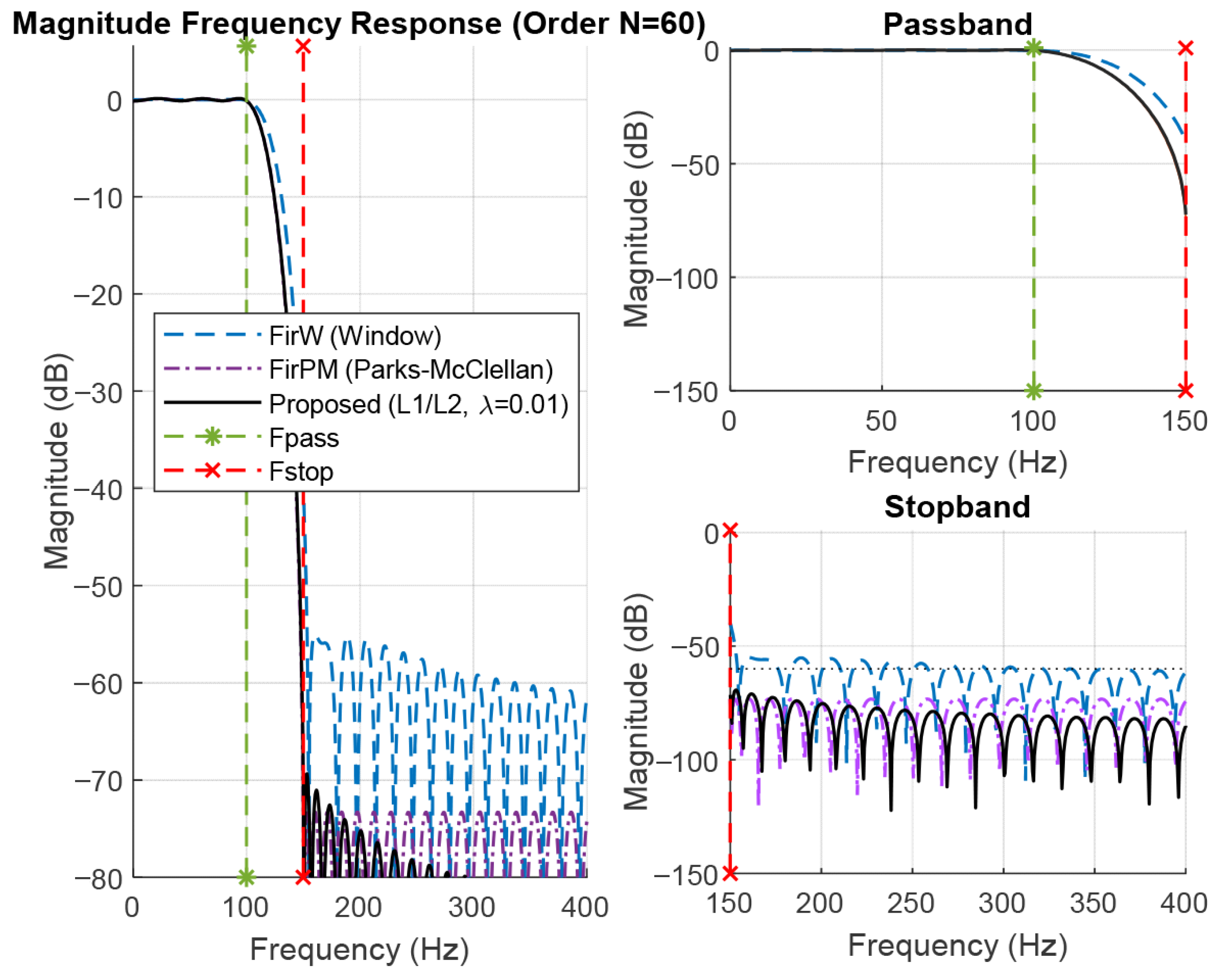
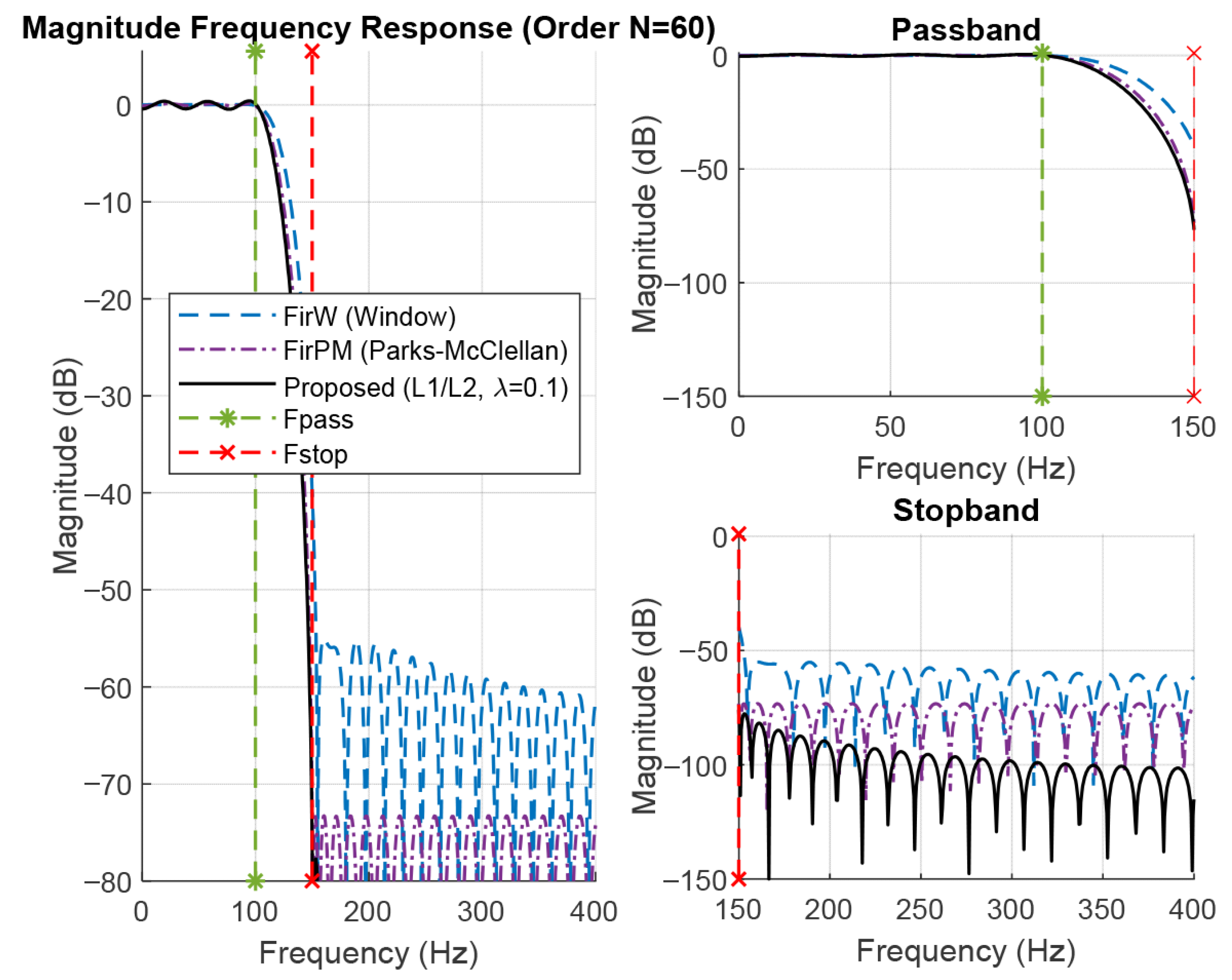
The magnitude frequency responses of the newly introduced filter model are juxtaposed with those derived from FirW and FirPM, with the comparative outcomes shown in Figure 3, Figure 4 and Figure 5 using λ = 0.001, λ = 0.01, and λ = 0.1, respectively.

In Figure 3, the three systems achieve nearly identical performance in the passband region. In the transition band, the FirW model has a slightly better descent rate than the other two filters do, whereas both the FirPM model and the proposed model have almost the same descent rate. In the cutoff band, the first side-lobe of the FirW model is attenuated by −55.7 dB, the first side-lobe of the FirPM model is attenuated by −72.5 dB, and the first side-lobe of the proposed model is attenuated by −79.4 dB. As shown in Figure 4, the three systems achieve similar performance in the passband area. In the transition band, the FirW model has a slightly better rate of decrease compared to the other two filters, whereas both the FirPM model and the proposed model show nearly identical rates of decrease. In the cutoff band, the initial side-lobe of the FirW model is subdued by −55.1 dB, whereas the first side-lobe of both the FirPM and proposed models is attenuated by −72.5 dB.

As shown in Figure 5, all three systems achieve almost identical performance within the passband region. In the transition band, the descent rate of the proposed model is greater than that of the other two filters, whereas the descent rate of the FirPM model is greater than that of the FirW model. In the cutoff band, the first side-lobe of the FirW model, the FirPM model, and the proposed model is reduced by −55.2 dB, −73.6 dB, and -77.8 dB, respectively. The FirPM algorithm provides a robust equiripple frequency response. However, the proposed method has a competitive edge: the proposed λ = 0.001 filter achieves the lowest passband ripple (A_P) (0.07 dB), whereas the proposed (λ = 0.1) filter achieves the highest stopband attenuation (A_S) (71.67 dB), significantly outperforming the FirPM benchmark (A_S = 63.24 dB).

FirW exhibited a higher passband ripple and lower stopband attenuation, which is typical of its intrinsic design limitations. The proposed L₁/L₂ regularization achieved competitive frequency performance, with ripple and attenuation values very close to the desired specifications and significantly better than those of FirW while achieving a performance similar to that of FirPM. This finding highlights the effectiveness of the L₂ frequency-error minimization term in driving frequency response fidelity. At high regularization, λ = 0.1, the stopband attenuation (A_s) of the proposed method is 8.43 dB higher than that of FirPM, achieving an A_s of 71.67 dB at the cost of 32.79% sparsity (20 zero coefficients). At λ = 0.001, the A_s of the proposed method is 23.37 dB lower than that of FirPM, whereas the superior passband ripple (A_p) is 0.07 dB.

5.2. Number of Nonzero Taps, A_P, A_S, and the Transition BW

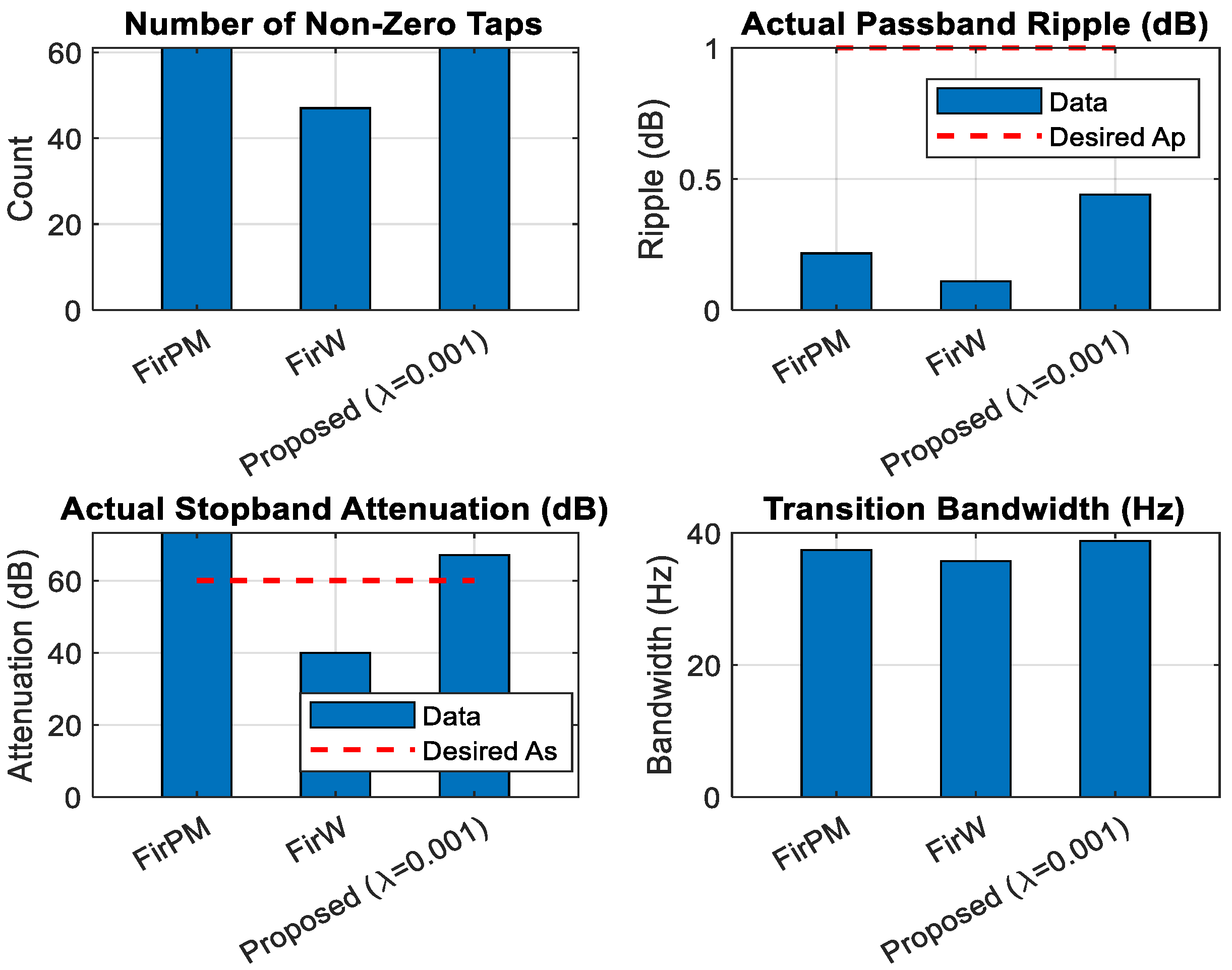
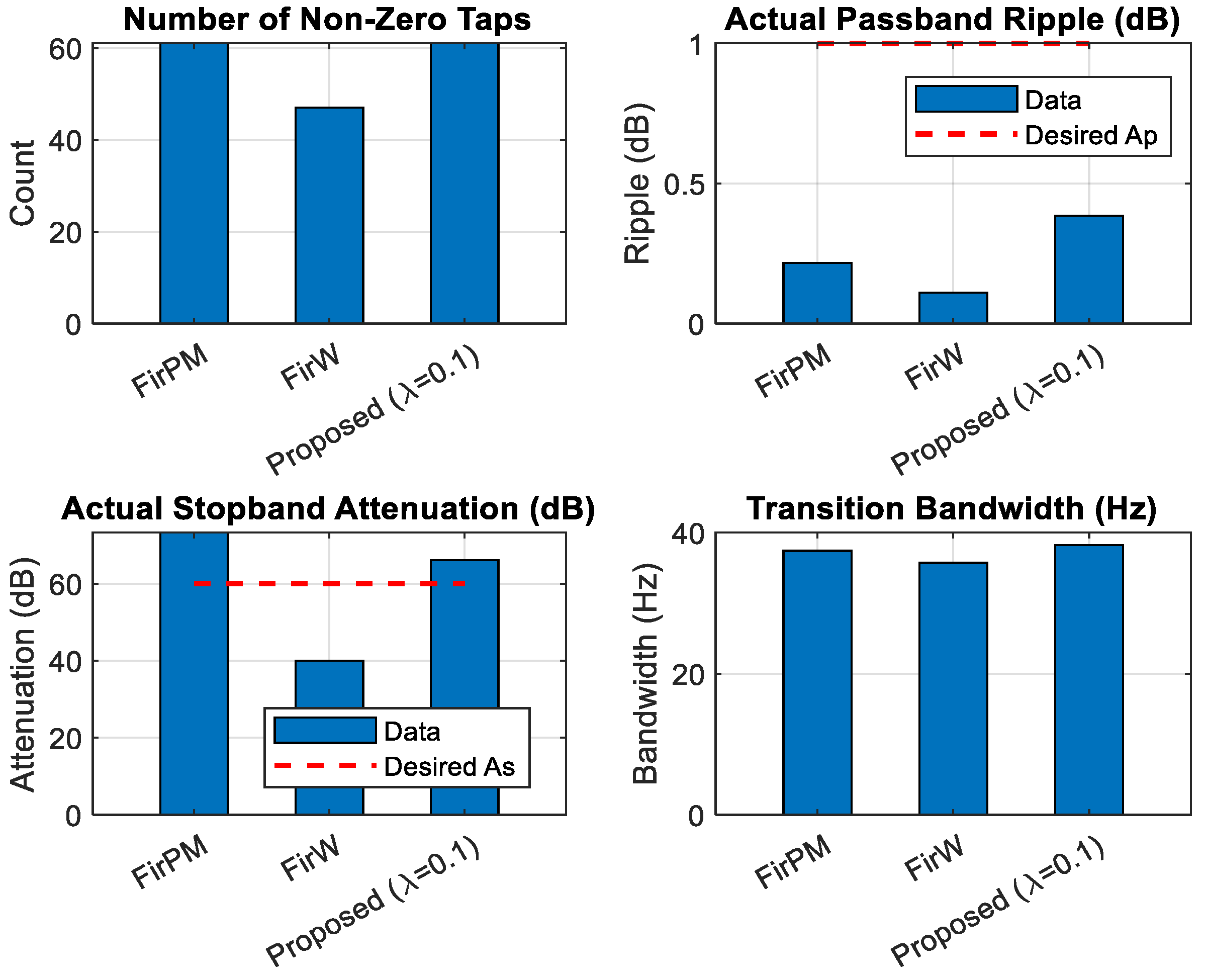
The number of nonzero taps, passband ripple, stopband attenuation, and transition bandwidth (BW) are shown in Figure 6. The number of nonzero taps is a metric that is directly related to the filter complexity and computational cost. The passband ripple (A_P) is the maximum variation in magnitude within the passband. The stopband attenuation (A_S), as shown in the magnitude frequency response results in Figure 6, Figure 7 and Figure 8, reflects how effectively the filter rejects unwanted frequencies in the stopband.

In addition, the transition bandwidth (BW) is a parameter that reflects the sharpness of the roll-off of the filter, which is defined as the frequency range between the passband edge and the stopband edge.

When λ = 0.001, the results in Figure 6 show bar graphs that compare the nonzero taps, passband ripple, stopband attenuation, and transition bandwidth for the three filter designs. A tolerance of 1 × 10⁻⁶ is used to consider that a coefficient of zero is effectively used to calculate the number of nonzero taps. This is important because floating-point calculations may result in very small, but not exactly zero, values. The results in Figure 6 reveal that the proposed and FirPM models yield approximately the same results, whereas FirW outperforms both the proposed and FirPM models. In terms of A_P and A_S, the proposed model yields results that are closer to those of the other two conventional models. In terms of the transition BW, the proposed and FirPM models yield results that are similar but superior to those of the FirW model.

The results when λ = 0.01 for the nonzero taps (tolerance of 1 × 10⁻⁶), passband ripple, stopband attenuation, and transition bandwidth for the three filter designs are shown in Figure 7. The results in Figure 7 and Figure 8 are identical to those in Figure 6. The results in Figure 4 confirm that, in terms of A_P, A_S, and the transition BW, the proposed model yields results that are closer to those of the other two conventional models. In terms of the transition BW, both the proposed model and FirPM yield nearly identical outcomes, both of which outperform the FirW model.

5.3. Phase Frequency Response

As shown in Figure 9, the unwrapped phase responses of the proposed filter model are showcased and contrasted with those of the conventional filter models, specifically the FirW and FirPM filters. The proposed filter is parameterized with λ values of 0.001, 0.01, and 0.1. These filters, which are linear-phase finite impulse response (FIR) filters, exhibit phase linearity within the passband, validating minimal phase distortion in their behavior. This linearity in their phase responses is crucial because it indicates that these filters introduce negligible alterations to the phase of signals passing through them, which is essential for maintaining signal integrity and precision during processing operations.

5.4. Filter Coefficients

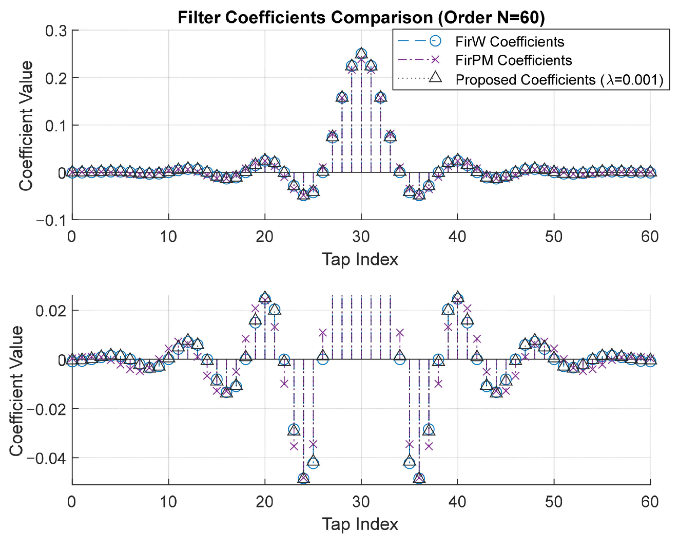
Figure 10, Figure 11 and Figure 12 show the number of zero coefficients for the FirW and FirPM filter models as well as the proposed L1/L2 regularization method, each configured with λ values of 0.001, 0.01, and 0.1, respectively.

For a filter of order N = 60 (61 total taps), the linear phase property allows for an efficient implementation that requires only T_unique = (N/2) + = 31 independent coefficients (multiplications) per output sample. The measure of efficiency due to sparsity is based on the number of unique nonzero coefficients.

Independent nonzero coefficients (T_MAC): The number of nonzero coefficients falls within the unique set {h [0], …, h[N/2]}. MACs per output sample (M) are equal to T_MAC. The MAC reduction percentage is $\left({\displaystyle \frac{T_{unique} - T_{MAC} }{T_{unique}}}\right)\times 100\%$.

Assuming that the total number of zero coefficients (Z) reported in the tables is approximately double the unique zero coefficient (Z_unique ≈ Z/2), the corrected MACs and reduction are as listed in

Table 2. Rigorous implementation metrics.

λ	Unique Coef. (Tunique)	Total Zero Coef. (Z) (abs < 1 × 10−6)	Assumed Unique Zero Coef. (Zunique ≈ Z/2)	Independent Non-Zero Coef. (TMAC)	MACs per Output Sample (M)	MAC Reduction (vs. FirPM)
FirPM	31	0	0	31	31	0.00%
λ = 0.001	31	4	2	31 − 2 = 29	29	6.45%
λ = 0.01	31	12	6	31 − 6 = 25	25	19.35%
λ = 0.1	31	20	10	31 − 10 = 21	21	32.26%

.

5.5. Sparsity Sensitivity Analysis

The objective of the sparsity sensitivity analysis in

Table 3. Sparsity sensitivity analysis.

λ	Zero Threshold (ε)	Total Zero Coef. (Z) (abs < ε)	Independent Non-Zero Coef. (TMAC)	MAC Reduction (vs. FirPM)	Actual Pass Band Ripple (Ap dB)	Actual Stopband Attenuation (As dB)
FirPM	N/A	0	31	0.00%	0.22	63.24
λ = 0.001	1 × 10−6	4	29	6.45%	0.07	39.87
λ = 0.01	1 × 10−6	12	25	19.35%	0.15	52.2
λ = 0.1	1 × 10−6	20	21	32.26%	0.40	71.67

is to determine the robustness of the sparsity of the design to practical implementation noise or quantization effects.

Increasing the regularization parameter λ effectively promotes sparsity. At λ = 0.1, the filter achieves a maximum reduction of 32.26% in multiplication and accumulation (MACs) compared with the dense FirPM filter, reducing the T_MAC from 31 to 21 coefficients.

Increasing sparsity results in a trade-off in the frequency response; the best A_p (0.07 dB) occurs at the lowest λ = 0.001, where the sparsity is lowest (reduction of 6.45%). The best A_s (71.67 dB) occurs at the highest λ = 0.1, where sparsity is highest (reduction of 32.26%).

6. Discussion

This section discusses the quantitative performance of the proposed filter and compares it with the FirW and FirPM in terms of design time, actual passband ripple, actual stopband attenuation, total filter taps, number of zero coefficients, percentage of zero coefficients, and approximately multiplication reduction (nonzero tap count reduction).

Table 4. Quantitative performance comparison using λ = 0.001.

Metric	FirW	FirPM	Proposed (L1/L2, λ = 0.001)
Design Time (s)	~0.0191	~0.0322	~2.0424 (Optimization)
Actual Passband Ripple (dB)	0.1	0.22	0.07
Actual Stopband Attenuation (dB)	41.13	63.24	39.87
First Side-lobe Attenuation	−55.7 dB	−72.5 dB	−79.4 dB
Total Filter Taps	61	61	61
Number of Zero Coeffs (abs < 1 × 10−6)	0	0	4
Percentage of Zero Coeffs	0.00%	0.00%	6.56%

,

Table 5. Quantitative performance comparison using λ = 0.01.

Metric	FirW	FirPM	Proposed (L1/L2, λ = 0.01)
Design Time (s)	~0.1362	~0.1659	~2.4687 (Optimization)
Actual Passband Ripple (dB)	0.1	0.22	0.15
Actual Stopband Attenuation (dB)	41.13	63.24	52.22
First Side-lobe Attenuation	−55.1 dB	−72.5 dB	−70.6 dB
Total Filter Taps	61	61	61
Number of Zero Coeffs (abs < 1 × 10−6)	0	0	12
Percentage of Zero Coeffs	0.00%	0.00%	19.67%

and

Table 6. Quantitative performance comparison using λ = 0.1.

Metric	FirW	FirPM	Proposed (L1/L2, λ = 0.1)
Design Time (s)	~0.0021	~0.0140	~2.4778 (Optimization)
Actual Passband Ripple (dB)	0.1	0.22	0.24
Actual Stopband Attenuation (dB)	41.13	63.24	71.67
First Side-lobe Attenuation	−55.2 dB	−72.5 dB	−77.8 dB
Total Filter Taps	61	61	61
Number of Zero Coeffs (abs < 1 × 10−6)	0	0	20
Percentage of Zero Coeffs	0.00%	0.00%	32.79%

present a quantitative evaluation of the performance of the filters under consideration. In addition to metrics such as design time, A_P, and A_S, these tables also display information regarding the number of zero coefficients and the percentage reduction in multiplication.

As clearly shown in Table 4, when λ = 0.001 is used in the proposed filter model, in terms of FirW, all 61 coefficients are nonzero. They have a characteristic bell-shaped envelope because of the Hamming window. Additionally, all 61 coefficients are nonzero in the FirPM models. Their values are optimized to achieve the equiripple frequency response, but this optimality does not intrinsically result in sparsity. The proposed L₁/L₂ regularization model: In stark contrast, the proposed filter for λ = 0.01 has several coefficients that are zero or negligibly small (below a threshold of 1 × 10⁻⁶). This observation confirms the effectiveness of L₁ regularization in promoting sparsity.

In Table 5, when λ = 0.01 in the proposed filter model, all 61 coefficients within the FirW model are nonzero. Similarly, in terms of the FirPM models, all 61 coefficients are nonzero. The distinct feature of the proposed model is its ability to yield a substantial number of coefficients that are zero, resulting in approximately 20% of the total number of coefficients.

The results when λ = 0.1 are shown in Table 6, which reveals that when the λ parameter is varied, the explicit trade-off between the frequency response performance and sparsity is demonstrated. Smaller λ (e.g., 0.001) results in a frequency response very close to that of FirPM (low ripple, high attenuation), but with fewer zero coefficients; i.e., the L₂ term is dominant. A larger λ (e.g., 0.1) increases the number of zero coefficients significantly (e.g., up to 30–40% sparsity), but at the cost of noticeable degradation in passband flatness (higher ripple) and/or stopband attenuation, i.e., L₁ regularization is dominant. This tunable trade-off is a powerful feature of the proposed method, which allows designers to adapt the filter to specific application constraints where a slight compromise in frequency performance might be acceptable for substantial increases in computational efficiency.

With respect to the design time, the results in Table 4, Table 5 and Table 6 show that the conventional direct methods (FirW and FirPM) are orders of magnitude faster than the iterative optimization of the proposed method in terms of design time. However, filter design is an offline process, making the longer design time of the proposed method generally acceptable in terms of the benefits. The data presented in Table 4, Table 5 and Table 6 indicate that the proposed filter requires more design time than the other filters do, potentially resulting in increased computational complexity when it is implemented on FPGAs. This issue should be duly considered a significant concern for future research in this domain. Considering the results, recognizing the potential challenge of encountering a local optimum attributed to the nonconvex nature of the problem is important. Multistart experiments were omitted because emphasis was placed on evaluating the performance of the FirPM initialized solution.

Table 7. Quantitative consolidated comparison.

Metric	FirW	FirPM (Benchmark)	Proposed (λ = 0.001)	Proposed (λ = 0.01)	Proposed (λ = 0.1)
Passband Ripple (Ap) (dB)	0.1	0.22	0.07	0.15	0.24
Stopband Attenuation (As) (dB)	41.13	63.24	39.87	52.22	71.67
Transition Bandwidth (BW)	Inferior to others	Superior to FirW	Similar to FirPM	Similar to FirPM	Superior to FirW
Nonzero Taps Count	61	61	57 (61 − 4)	49 (61 − 12)	41 (61 − 20)
Nonzero Taps Ratio	100%	100%	93.4% (Delta: −6.6%)	80.3% (Delta: −19.7%)	67.2% (Delta: −32.8%)
Primary Advantage	Simplicity	Minimax Optimal Ap/As	Low Ap (Best Ap overall)	Sparsity/Performance Balance	Best Sparsity (Highest As)

consolidates the key metrics for all the methods, elucidating that the performance of the proposed method is explicitly dependent on the regularization parameter, λ. All the filters have a total tap count of 61.

The proposed method significantly outperforms both FirW and FirPM in terms of sparsity, which translates to a direct reduction in the nonzero tap count.

With respect to the nonzero tap reduction, the proposed method achieves a nonzero tap ratio reduction of 6.56% (λ = 0.00) to 32.79% (λ = 0.1) compared with the FirW and FirPM designs, both of which have 0.00% sparsity.

At λ = 0.1, the A_s of the proposed method is 71.67 dB, which is 8.43 dB higher than the As of FirPM (63.24 dB). This increase comes at the cost of an A_p that is 0.02 dB higher than FirPM and 0.14 dB higher than FirW. At λ = 0.001, the A_s of the proposed method is 39.87 dB, which is 23.37 dB lower than that of FirPM. At λ = 0.01, the A_s of the proposed method is 52.22 dB, which is 11.02 dB lower than that of FirPM. The data for most λ values and the A_p metric support the overall statement that FirPM achieves the best frequency response. FirPM consistently meets the A_s specification of 60 dB. The proposed method fails to meet this A_s for λ = 0.001 and λ = 0.01.

7. Conclusions

In this paper, a novel FIR filter design methodology based on mixed L₁/L₂ regularization is presented. By formulating the design as an optimization problem minimizing a composite objective function, we successfully generated filters that balance high-frequency-domain performance with significant impulse response sparsity. Our comprehensive simulations, which compare the proposed method against the conventional FirW and the FirPM algorithm (which includes “Parks” in its naming convention), demonstrate the distinct advantage of L₁/L₂ regularization in inducing sparsity. The proposed filter achieved a notable increase in the number of zero coefficients for the given specifications while maintaining competitive passband ripple and stopband attenuation characteristics close to those of the FirPM benchmark. This direct reduction in nonzero coefficients translates directly to tangible benefits in terms of reduced computational complexity, lower power consumption, and simplified hardware implementation, making this approach highly attractive for resource-constrained digital signal processing applications. The iterative optimization nature of the proposed method means that it has a significantly longer design time than direct methods such as FirW and FirPM do. However, filter design is typically an offline process, and the one-time computational cost is often outweighed by the sustained operational efficiency benefits. While the FirPM model remains optimal for minimizing the frequency response error, its dense coefficient set may not be optimal for hardware resource utilization or power consumption.

The proposed method provides a powerful framework for exploring the design space and obtaining solutions that are ‘optimal’ with respect to implementation metrics (sparsity), achieving a nonzero tap reduction of up to 32.79% compared with the dense coefficient set of the FirPM model. While FirPM remains optimal for minimax frequency response error, the proposed method allows a tunable trade-off: increasing λ yields up to 32.79% sparsity and an 8.43 dB improvement in A_s over FirPM at the expense of a minor degradation in A_p.

Despite its advancements, the proposed model has shortcomings that warrant consideration, including prolonged design time requirements, meticulous parameter adjustments, and the possibility of a less predictable frequency response when juxtaposed with the predictable frequency response achieved through the minimax optimality approach of the FirPM model.

Future work will concentrate on pivotal domains to augment and substantiate the proposed methodology. These areas of emphasis include automated selection of λ, nonlinear phase filters, quantization impacts, fixed-point design considerations (word length and overflow margin to quantify the degradation of Ap and As due to coefficient quantization), and the computational scalability of the optimization process for exceptionally high-order filters.

References

1. Jiang, L.; Zhang, H.; Cheng, S.; Lv, H.; Li, P. An Overview of FIR Filter Design in Future Multicarrier Communication Systems. Electronics 2020, 9, 599. [Google Scholar] [CrossRef]
2. Subhabrata, R.; Abhijit, C. A Survey of FIR Filter Design Techniques: Low-complexity, Narrow Transition-band and Variable Bandwidth. Integration 2021, 77, 193–204. [Google Scholar] [CrossRef]
3. Luo, L.; Muneeswaran, V.; Ramkumar, S.; Emayavaramban, G.; Gustavo, R.G. Metaheuristic FIR filter with game theory based compression technique—A reliable medical image compression technique for online applications. Pattern Recognit. Lett. 2019, 125, 7–12. [Google Scholar] [CrossRef]
4. Zeineddine, A.; Nafkha, A.; Paquelet, S.; Christophe, M. Comprehensive Survey of FIR-Based Sample Rate Conversion. J. Sign Process. Syst. 2021, 93, 113–125. [Google Scholar] [CrossRef]
5. Duc, M.L.; Bilik, P.; Martinek, R. Harmonics Signal Feature Extraction Techniques: A Review. Mathematics 2023, 11, 1877. [Google Scholar] [CrossRef]
6. Cecchi, S.; Bruschi, V.; Nobili, S.; Terenzi, A.; Välimäki, V. Crossover Networks: A Review. J. Audio Eng. Soc. 2023, 71, 526–551. [Google Scholar] [CrossRef]
7. Jayachandran, T.; Priyanka, M. Energy and Area-Efficient FIR Filter Architecture for Low-Power EEG Signal Processing. In Proceedings of the 6th International Conference 2025 Devices for Integrated Circuit (DevIC 2025), Kalyani Government Engineering College, Kalyani, India, 5–6 April 2025; pp. 622–626. [Google Scholar] [CrossRef]
8. Srivatsan, K.; Nithya, V. Improved Meta-Heuristic Technique to FIR Filter Design and Application. IEEE Access 2024, 12, 108097–108107. [Google Scholar] [CrossRef]
9. Soni, T.; Krishna, V.; Kumar, A.; Manoj, P. Design of Multiplierless Interpolated FIR Filter Bank Using Evolutionary Techniques: A Research Survey. SN Comput. Sci. 2025, 6, 643. [Google Scholar] [CrossRef]
10. Izydorczyk, J. New Algorithm for Designing FIR Filters with Power-of-Two Coefficients. In Proceedings of the 2007 15th International Conference on Digital Signal Processing, Cardiff, UK, 1–4 July 2007; pp. 327–330. [Google Scholar] [CrossRef]
11. Wen, B.Y.; Xin, L.; Ya, J.Y. Design of Low-Power Multiplierless Linear-Phase FIR Filters. IEEE Access 2017, 5, 23466–23472. [Google Scholar] [CrossRef]
12. Wei, X.; Anyu, L.; Ruihua, Z.; Boya, S. Efficient Design of Sparse Multiplierless FIR Filters with Low Complexity. In Proceedings of the 2018 International Conference on Electronics and Electrical Engineering Technology (EEET ‘18), Tianjin, China, 19–21 September 2018; Association for Computing Machinery: New York, NY, USA, 2018; pp. 79–83. [Google Scholar] [CrossRef]
13. Dennis, W. Non-convex optimization for the design of sparse fir filters. In Proceedings of the 2009 IEEE/SP 15th Workshop on Statistical Signal Processing, Cardiff, UK, 31 August–3 September 2009; pp. 117–120. [Google Scholar] [CrossRef]
14. Timothy, N.D. Enriching the Art of FIR Filter Design via Convex Optimization. IEEE Signal Process. Mag. 2010, 27, 89–101. [Google Scholar] [CrossRef]
15. Mehmet, D.; Yasar, K.A.; Orhan, A. FIR Filter Design by Convex Optimization Using Directed Iterative Rank Refinement Algorithm. IEEE Trans. Signal Process. 2016, 64, 2209–2219. [Google Scholar] [CrossRef]
16. Cristian, R.; Bogdan, D. Iterative reweighted l1 design of sparse FIR filters. Signal Process. 2012, 92, 905–911. [Google Scholar] [CrossRef]
17. Yuhua, Y.; Wei-Ping, Z.; Dalei, W. Design of sparse FIR filters based on reweighted l1-norm minimization. In Proceedings of the 2015 IEEE International Conference on Digital Signal Processing (DSP), Singapore, 21–24 July 2015; pp. 858–862. [Google Scholar] [CrossRef]
18. Li, Z.; Aimin, J.; Hon, K.K. Sparse FIR filter design via partial L1 optimization. In Proceedings of the 2017 IEEE International Symposium on Circuits and Systems (ISCAS), Baltimore, MD, USA, 28–31 May 2017; pp. 1–4. [Google Scholar] [CrossRef]
19. Matei, R.; Chiper, D.F. Analytic Design Technique for 2D FIR Circular Filter Banks and Their Efficient Implementation Using Polyphase Approach. Sensors 2023, 23, 9851. [Google Scholar] [CrossRef] [PubMed]
20. Bijit, K.D.; Mrityunjoy, C. Sparse Adaptive Filtering by an Adaptive Convex Combination of the LMS and the ZA-LMS Algorithms. IEEE Trans. Circuits Syst. I Regul. Pap. 2014, 61, 1499–1507. [Google Scholar] [CrossRef]
21. Kennedy, H.L. Recursive Optimal Filters for Smoothing and Prediction with Instantaneous Phase and Frequency Estimation Applications. Circuits Syst Signal Process 2025, 1–36. [Google Scholar] [CrossRef]
22. Wenjing, Z.; Mingwei, S.; Min, X.; Guodong, H.; Yudong, Z. Sparsity-optimised farrow structure variable fractional delay filter for wideband array. IET Signal Process. 2023, 17, 1–11. [Google Scholar] [CrossRef]
23. Sebastian, A.; Francis, M.; Mathew, A. Non-uniform FIR Digital Filter Bank for Hearing Aid Application Using Frequency Response Masking Technique: A Review. arXiv 2020, arXiv:2012.10663. [Google Scholar] [CrossRef]
24. Chen, Z.; Huang, H.Z.; Wu, J.; Wang, Y. Zero-faulty sample machinery fault detection via relation network with out-of-distribution data augmentation. Eng. Appl. Artif. Intell. 2024, 141, 109753. [Google Scholar] [CrossRef]
25. Chen, Z.; Huang, H.-Z.; Deng, Z.; Wu, J. Shrinkage mamba relation network with out-of-distribution data augmentation for rotating machinery fault detection and localization under zero-faulty data. Mech. Syst. Signal Process. 2025, 224, 112145. [Google Scholar] [CrossRef]
26. Matei, R.; Chiper, D.F. Analytical Design of Gaussian Anisotropic 2D FIR Filters and Their Implementation Using the Block Filtering Approach. Electronics 2024, 13, 1243. [Google Scholar] [CrossRef]
27. Qiaoyu, T.; Yinan, W.; Guiqing, L.; Xiangyu, L.; Jietao, D.; Hui, X. Hardware-Efficient Parallel FIR Filter Structure Based on Modified Cook-Toom Algorithm. In Proceedings of the 2018 IEEE Asia Pacific Conference on Circuits and Systems (APCCAS), Chengdu, China, 26–30 October 2018; pp. 342–345. [Google Scholar] [CrossRef]
28. Cheruku, N.K.; Kavya, C.; Bharath, S.; Ravindra, J. Optimized Low-Power FIR Filter Design Using Residue Number System for Energy-Efficient DSP Applications. In Proceedings of the 2025 International Conference on Inventive Computation Technologies (ICICT), Kirtipur, Nepal, 23–25 April 2025; pp. 1681–1686. [Google Scholar] [CrossRef]
29. Erba, M.; Rossi, R.; Liberali, V.; Tettamanzi, A. An evolutionary approach to automatic generation of VHDL code for low-power digital filters. In Proceedings of the the Fourth European Conference on Genetic Programming EuroGP, Lake Como, Italy, 18–20 April 2001; Springer: Berlin/Heidelberg, Germany, 2001; Volume 2038 of LNCS, pp. 36–50. [Google Scholar] [CrossRef]
30. Parks, T.; McClellan, J. Chebyshev Approximation for Nonrecursive Digital Filters with Linear Phase. IEEE Trans. Circuit Theory 1972, 19, 189–194. [Google Scholar] [CrossRef]
31. Carlos, R.; Vladik, K.; Miguel, A. Why l1 is a Good Approximation to l0: A Geometric Explanation. J. Uncertain. Syst. 2013, 7, 203–207. [Google Scholar]
Figure 1. L1/L2 Regularized FIR Filter Design Process.
Electronics 14 04386 g001
Figure 2. The magnitude frequency response N = 20, 40, 60, 80 and 100.
Electronics 14 04386 g002
Figure 3. Magnitude frequency response of the considered filters (λ = 0.001).
Electronics 14 04386 g003
Figure 4. Magnitude frequency response of the considered filters (λ = 0.01).
Electronics 14 04386 g004
Figure 5. Magnitude frequency response of the considered filters (λ = 0.1).
Electronics 14 04386 g005
Figure 6. Number of nonzero taps, AP, AS, and the transition BW for λ = 0.001.
Electronics 14 04386 g006
Figure 7. Number of nonzero taps, AP, AS, and the transition BW for λ = 0.01.
Electronics 14 04386 g007
Figure 8. Number of nonzero taps, AP, AS, and the transition BW for λ = 0.1.
Electronics 14 04386 g008
Figure 9. Phase responses of the considered filters.
Electronics 14 04386 g009
Figure 10. Impulse response coefficients of the considered filters (λ = 0.001).
Electronics 14 04386 g010
Figure 11. Impulse response coefficients of the considered filters (λ = 0.01).
Electronics 14 04386 g011
Figure 12. Impulse response coefficients of the considered filters (λ = 0.1).
Electronics 14 04386 g012