Adversarial Defense for Medical Images

Abstract

The rapid advancement of deep learning is significantly hindered by its vulnerability to adversarial attacks, a critical concern in sensitive domains like medicine where misclassification can have severe, irreversible consequences. This issue directly underscores prediction unreliability and is central to the goals of Explainable Artificial Intelligence (XAI) and Trustworthy AI. This study addresses this fundamental problem by evaluating the efficacy of denoising techniques against adversarial attacks on medical images. Our primary objective is to assess the performance of various denoising models. The authors generate a test set of adversarial medical images using the one-pixel attack method, which subtly modifies a minimal number of pixels to induce misclassification. The authors propose a novel autoencoder-based denoising model and evaluate it across four diverse medical image datasets: Derma, Pathology, OCT, and Chest. Denoising models were trained by introducing Impulse noise and subsequently tested on the adversarially attacked images, with effectiveness quantitatively evaluated using standard image quality metrics. The results demonstrate that the proposed denoising autoencoder model performs consistently well across all datasets. By mitigating catastrophic failures induced by sparse attacks, this work enhances system dependability and significantly contributes to the development of more robust and reliable deep learning applications for clinical practice. A key limitation is that the evaluation was confined to sparse, pixel-level attacks; robustness to dense, multi-pixel adversarial attacks, such as PGD or AutoAttack, is not guaranteed and requires future investigation.

1. Introduction

1.1. Background

The rapid evolution of machine learning technology over time has led to the emergence of various network models. However, despite these advances, deep neural networks (DNNs) are still susceptible to adversarial attacks, which consist of adding adversarial samples to datasets to cause the model to make incorrect predictions. Numerous attack methods, including the Fast Gradient Sign Method (FGSM) [1], Box-Constrained L-BFGS [2], and one-pixel attacks [3], generate adversarial images by introducing malicious perturbations to images. The latter type appears to have garnered the most attention due to their ability to achieve adversarial effects by modifying a minimal number of pixels. In order to counter these effects, many denoising models have been developed to prevent adversarial images from being subject to such attacks by incorporating noise during training, followed by denoising to reconstruct and restore images to their original form. Examples of these models include Noise2Void [4] and Noise2Noise [5]. Additionally, other methods like trigger detection and candidate detection [6] are used to identify pixels that have potentially been tampered with. Adversarial training [7] is another common defense method, in which the model is trained with adversarial samples to enhance its resistance to attacks.

The rapid progress of machine learning has made many tasks easier, with its applications ranging across various fields to ease daily burdens. A prime example is the medical sector, where machine learning models are used to improve the efficiency of diagnoses. However, a significant risk arises from adversarial samples, which can cause a model to make a critical misjudgment, leading to severe consequences. This vulnerability has spurred the development of defense mechanisms and denoising models specifically for medical images.

Beyond standard adversarial training, other methods have been introduced, such as using variational auto encoders to detect one-pixel attacks in mammography images and to restore the original appearance of medical images through denoising and reconstruction [8,9]. While a variety of defense methods against one-pixel attacks exist, they are primarily designed for non-medical image datasets. Consequently, there is a considerable need for further research and development in detecting and restoring medical images that have been tampered with other research [10,11].

1.2. Research Goal

This study aims to restore medical images that are subject to pixel attacks to their original state by adding noise to different models during training for denoising, and to propose an improved denoising autoencoder model that effectively enhances the recovery of images post-attack. Experiments are conducted on four of the original datasets of medMNIST, namely, Chest, OCT, Derma, and Pathology. This study analyzes and compares the efficacy of adversarial attacks and denoising techniques across various medical image datasets. The datasets, which include binary, multi-label, and multi-class classification types, comprise images from diverse modalities such as X-rays, optical coherence tomography (OCT), dermoscopy, and histology. The selection of these specific datasets is motivated by several key factors.

1.2.1. Diverse Imaging Characteristics

These modalities represent a broad spectrum of medical imaging techniques, each with unique data characteristics. X-ray images, for instance, are based on the absorption of ionizing radiation and often have low contrast, while OCT images are high-resolution, cross-sectional views of tissue captured with light. Dermoscopy provides magnified surface-level views of the skin, and histology offers microscopic images of tissue at the cellular level. Evaluating adversarial and denoising methods across this diverse range allows for a more comprehensive understanding of their generalizability and robustness.

1.2.2. Vulnerability and Noise Profiles

Each modality is susceptible to different types of noise and artifacts. OCT images are particularly prone to speckle noise, a granular artifact that can obscure fine details. Histology images, created from tissue sections on slides, can contain artifacts from the staining and processing steps, such as tears, folds, or inconsistent staining. X-ray and dermoscopy images can be affected by patient motion, improper lighting, and variations in equipment. By including these distinct noise profiles, the study can assess the effectiveness of denoising algorithms in different challenging scenarios.

1.2.3. Clinical Significance

The chosen modalities are critical for diagnosing and managing a wide range of diseases. X-rays are foundational for detecting fractures, lung infections, and tumors. OCT is vital for diagnosing retinal diseases like diabetic retinopathy and glaucoma. Dermoscopy is a key tool for the early detection of skin cancer. Histopathology remains the gold standard for cancer diagnosis. The potential for adversarial attacks to manipulate AI-driven diagnostic systems in these critical areas highlights the importance of this research in ensuring the safety and reliability of clinical AI applications.

1.2.4. Data Availability and Complexity

The availability of public datasets for these modalities allows for replicable and comparable research. The datasets also offer different levels of classification complexity, from simple binary tasks (e.g., Normal Vs. Abnormal on an X-ray) to more complex multi-class and multi-label problems (e.g., classifying different types of skin lesions in dermoscopy or various tissue types in histology). This range of complexity enables a thorough evaluation of the models’ resilience to attacks and their performance improvements with denoising.

Therefore, the study is expected to make the following contributions:

• The proposal of an improved denoising autoencoder model.
• A demonstration that the proposed denoising model facilitates a better performance.
• The proposed method regarding detecting one-pixel attacks is better than existing research.

2. Related Works

2.1. One-Pixel Attacks

Of the many different types of adversarial attacks that have been developed in the field of deep learning in recent years, the one-pixel attack has drawn significant attention. These attacks primarily entail the introduction of slight perturbations to the input images, causing the model to produce incorrect results. Early one-pixel attack researchers used a differential evolution algorithm [3,12] to carry out the attacks, which only resulted in perturbing a single pixel in the image to generate an adversarial image. Then, it was found that there was high probability that one-pixel attacks could still successfully deceive the model, despite the original image retaining a certain level of classification confidence.

Additionally, Liu et al. [13] proposed a pixel-level adversarial attack method (Pixel-level Adversarial Attack, PIAA) in 2022, to highlight the issue of excessive perturbation in existing adversarial attacks, which made them detectable by the human eye. PIAA utilized an attention mechanism and pixel-level perturbation to more accurately select sensitive pixels, and then incrementally modified those pixels to generate adversarial samples that effectively attacked DNNs. On the other hand, the differential evolution algorithm generated adversarial samples based on various genotypes and crossover operations. For instance, Tsai et al. [14] investigated one-pixel and multi-pixel level attacks on a Deep Neural Network (DNN) model trained on a variety of medical image datasets. Likewise, Dietrich, Gong and Patlas [15] implemented adversarial artificial intelligence in radiology to test attacks, defenses on diagnostic and interventional imaging. Doshi et al. [16] and Dayarathna et al. [17] applied deep learning approach for biomedical image classification. Gong [18] implemented 3D biomedical image segmentation, classification to conclude detection. Ma et al. [19] processed U-mamba to enhance long-range dependency for biomedical image segmentation. Upadhyay [20] implemented machine learning-based and deep learning-based intrusion detection system.

2.2. Denoising Models in Image Applications

There are many denoising models in the field of machine learning that can restore damaged or attacked images to their original state by adding and removing noise. For instance, Krull et al. [4] introduced a method for training denoising neural networks called Noise2Void in 2019, which does not require clean ground truth data for training, but uses noisy images instead. The special architecture in Noise2Void, known as a blind-spot network, excludes the information of one pixel from that of its surrounding pixels, thereby preventing the neural network from merely memorizing the original value of the input pixel. Instead, the network learns the related information from the surrounding pixels, thereby enhancing the denoising effect.

Nasrin et al. [21] proposed a deep learning-based autoencoder model (R2U-Net base Auto-Encoder) in 2019, which consisted of a combination of the features of R2U-Net and autoencoders. Zhang et al. [22] proposed another denoising model in 2022 called the Swin-Conv-UNet (SC-UNet). A novel Swin-Conv (SC) block was the primary building module incorporated into the UNet architecture. The SC block combined the local modeling capability of the Residual Convolutional Layer (RConv) and the non-local modeling capability of the Swin Transformer Block (SwinT), thereby enhancing its capacity to model features. The experimental results indicated that the SC-UNet achieved better PSNR results under different noise levels and exhibited a good visual effect in denoising images.

2.3. Methods to Restore Images After Adversarial Attacks

In response to increasingly frequent adversarial attacks, scholars have attempted to restore the parts of adversarial images that have been tampered with to their original state, regardless of the type of image. Chen et al. [5] proposed a method called Patch Selection Denoise in 2019. This method achieved defense by removing potential attack pixels in local areas without having to alter many pixels in the whole image. This method comprised a combination of the Noise2Noise model and a patch selection algorithm. It trained the denoising model based on the Noise2Noise framework by generating noisy images by adding random-valued impulse noise to clear images. The patch selection algorithm then scanned the denoised image using a patch window and compared it with the corresponding part of the original image. If the absolute difference in the pixels in the patch greatly exceeded a preset threshold, the patch in the denoised image replaced the corresponding patch. The method was validated by the use of the public dataset CIFAR-10 in order to effectively detect pixels that had been tampered with and restore them to their original state.

Liang et al. [23] also proposed a new type of deep fully convolutional neural network in 2019 called MedianDenoise, In 2021, Husnoo et al. [24] proposed an image restoration algorithm based on the Accelerated Proximal Gradient approach to counter one-pixel attacks. This method involved transforming adversarial images into matrix formats and utilizing sparse matrix separation techniques to separate adversarial pixels, restoring the original image. The method optimized the problematic Robust Principal Component Analysis (RPCA) by minimizing the proximal gradient approximation. This defense mechanism aimed to restore the original image to protect it from adversarial attacks. According to the experimental results, this reconstruction algorithm could effectively mitigate one-pixel attacks on more advanced neural networks and worked effectively on CIFAR-10 and MNIST datasets.

In 2022, Alatalo et al. [8] utilized a variational autoencoder to reconstruct attacked images by first inputting the original image into the variational autoencoder to encode and decode it to obtain a reconstructed and clean image. They then calculated the difference between the original and reconstructed images and used it as an anomaly score. If this score exceeded a preset threshold, it could be determined that the image had been tampered with. In 2024, Surekha et al. [25] and Irede [26] conducted a thorough review on adversarial attack and defense mechanisms in medical imaging to compare the pros and cons. Likewise, Dong et al. [27] conducted surveys on adversarial attack and defense for medical image analysis. Haque et al. [28] proposed adversarial proof disease detection in radiology images.

In 2025, Budathoki and Manish [29] intended to implement adversarial attack for the vision language segmentation models (VLSMs). Zhao et al. [30] further adapted large-vocabulary segmentation for medical images with text prompts to make the best decision. Zheng [31] developed a generalist radiology diagnosis system regarding disease diagnosis on radiology images.

3. Methodology

3.1. Theoretical Basis

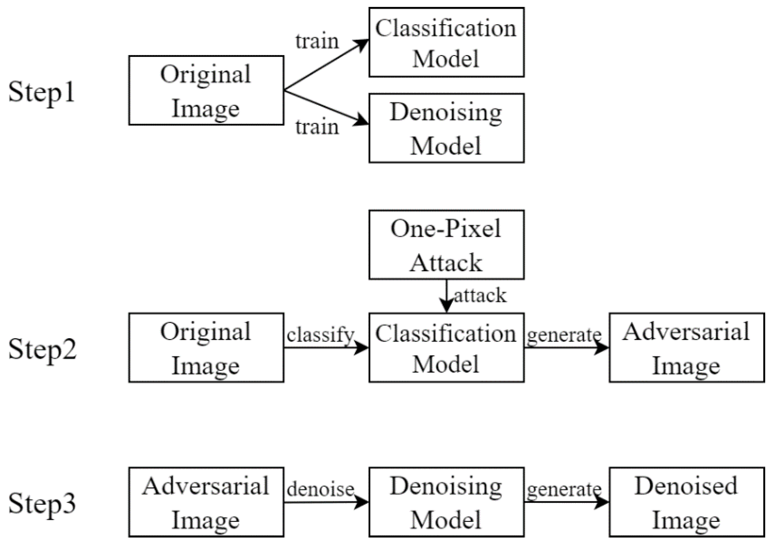
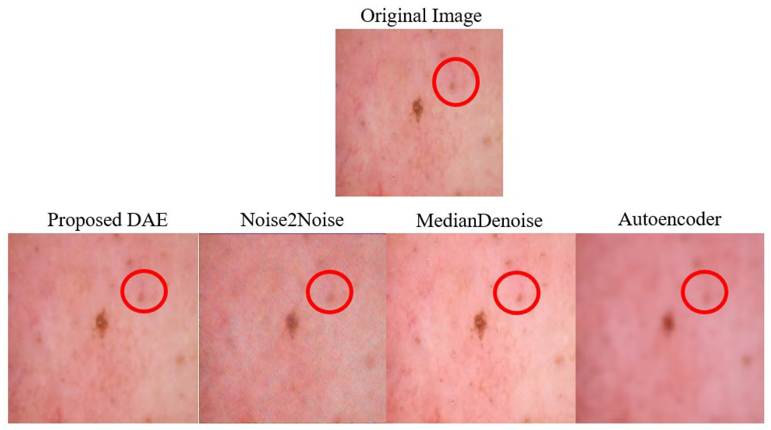
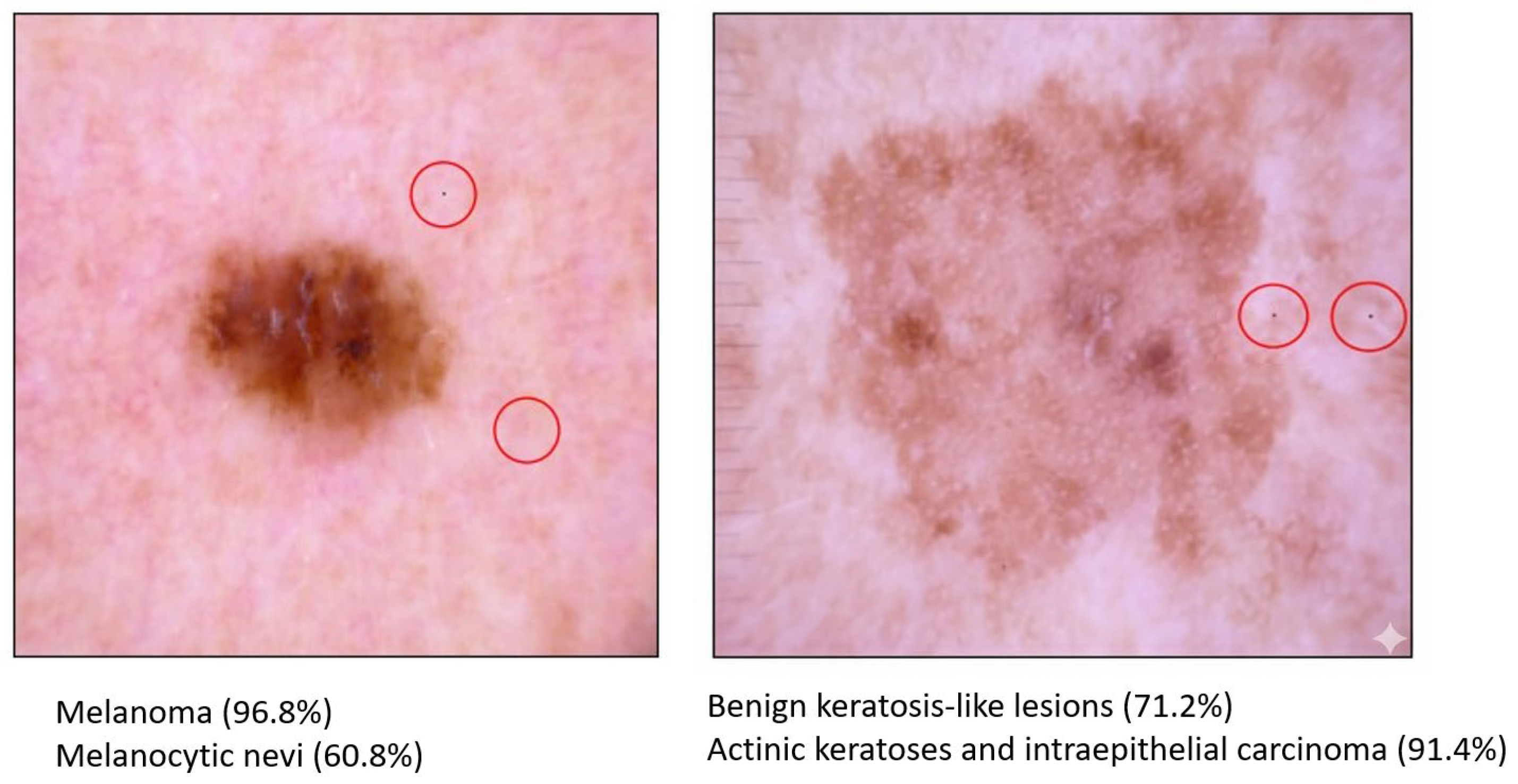
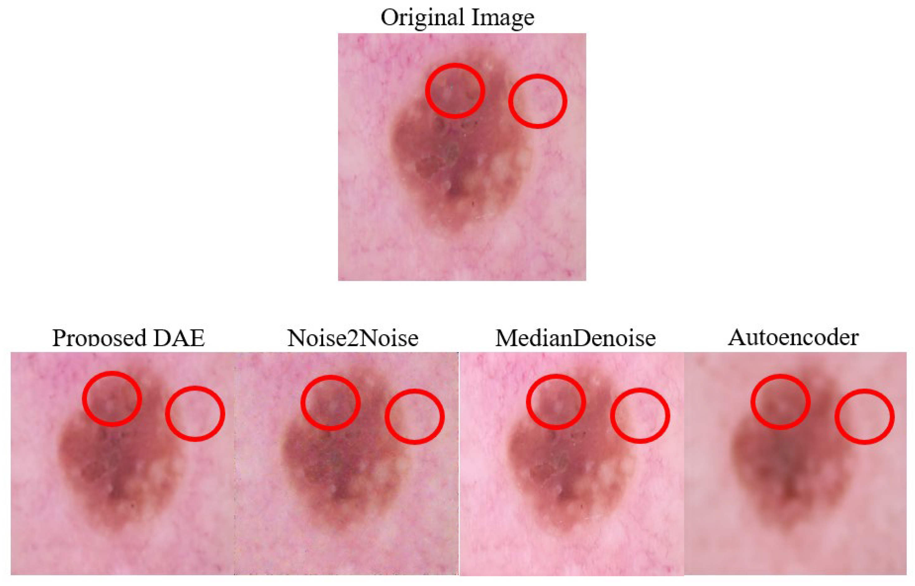
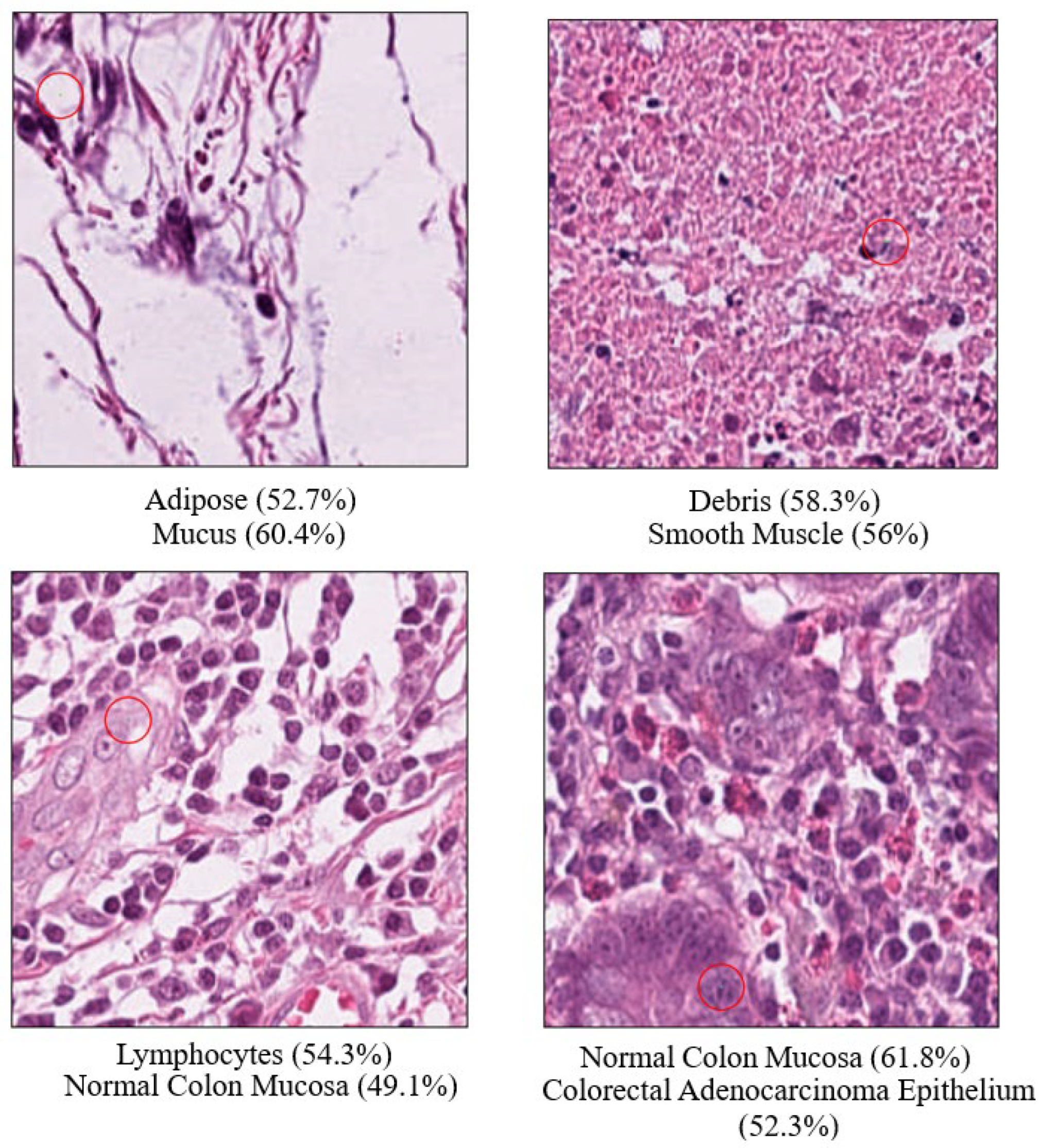
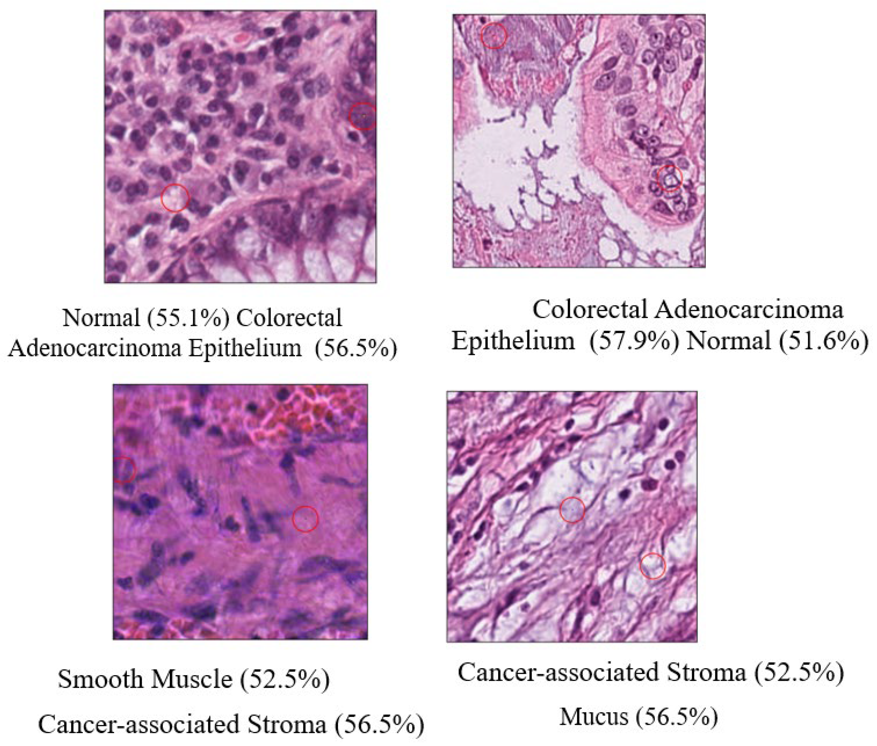
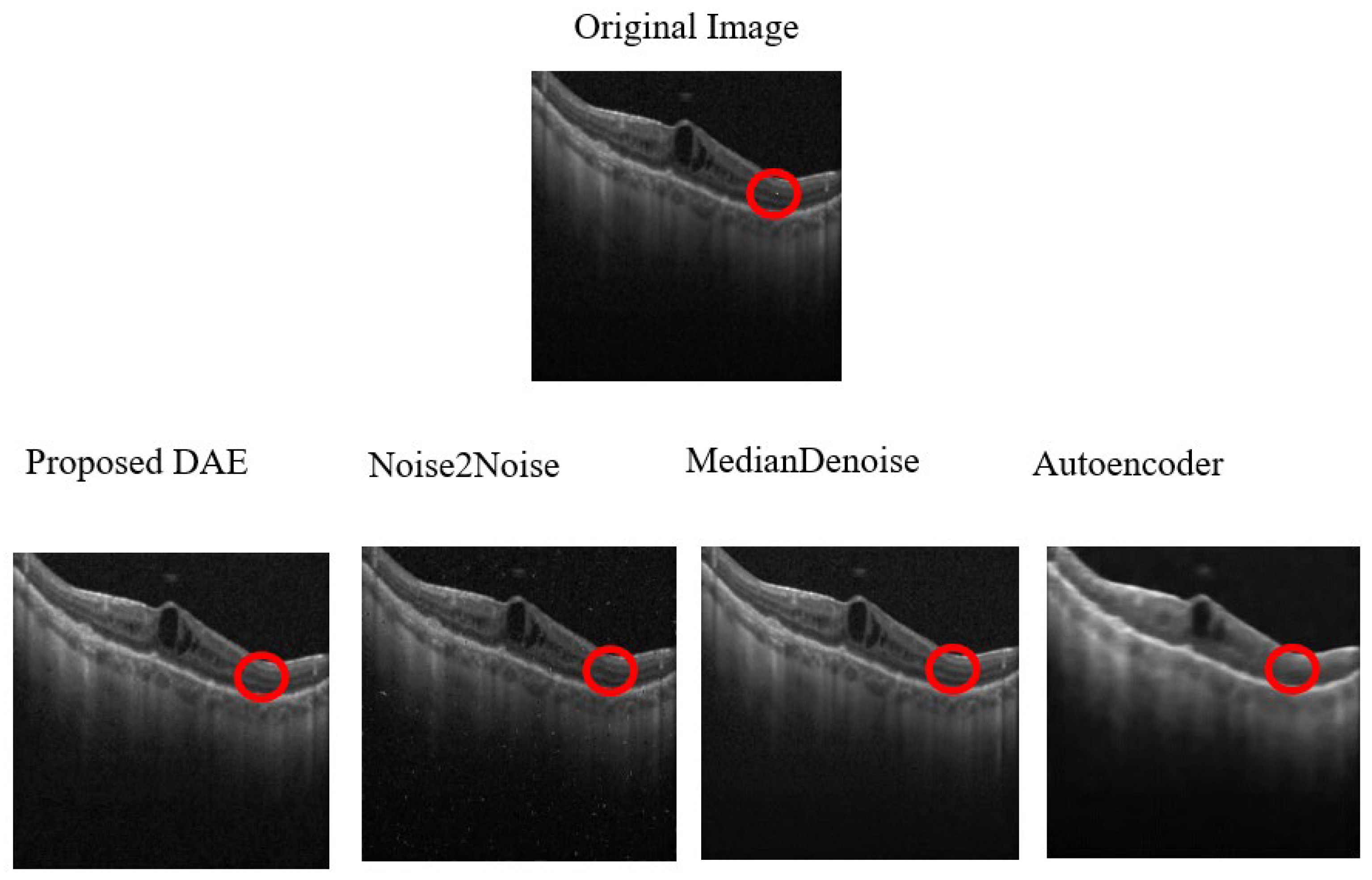
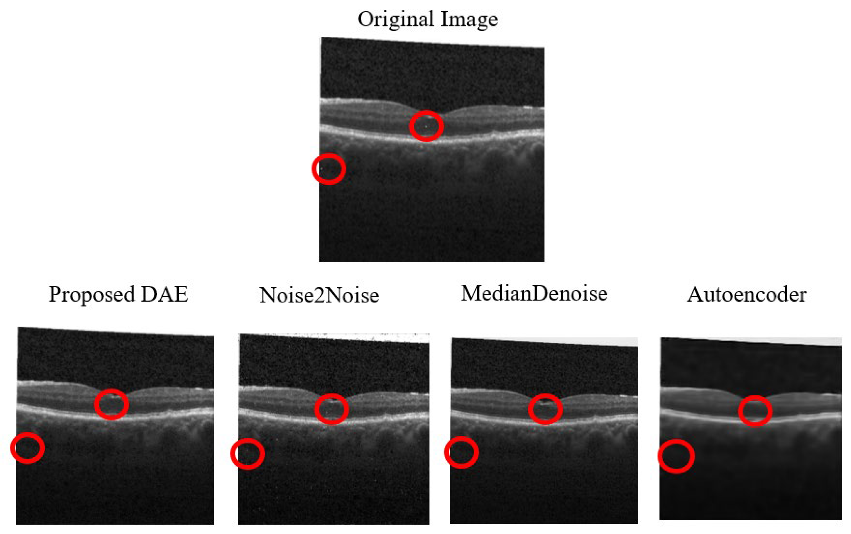
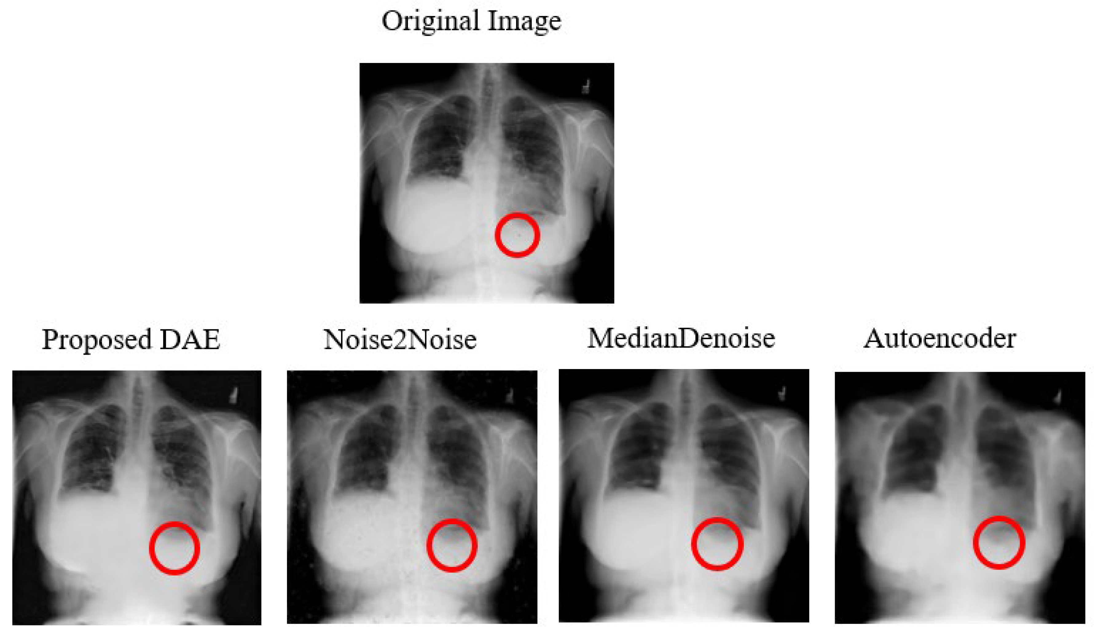
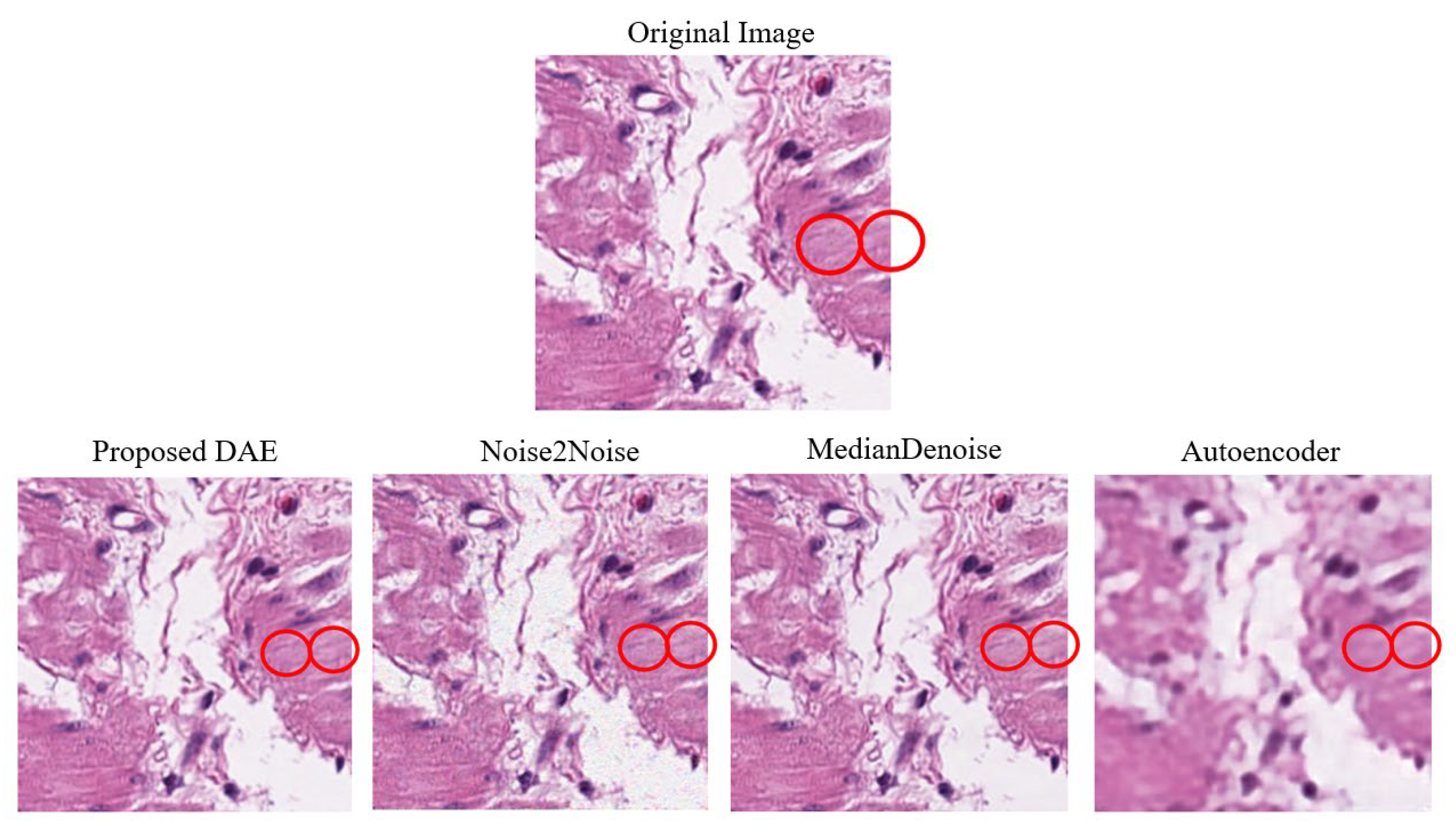
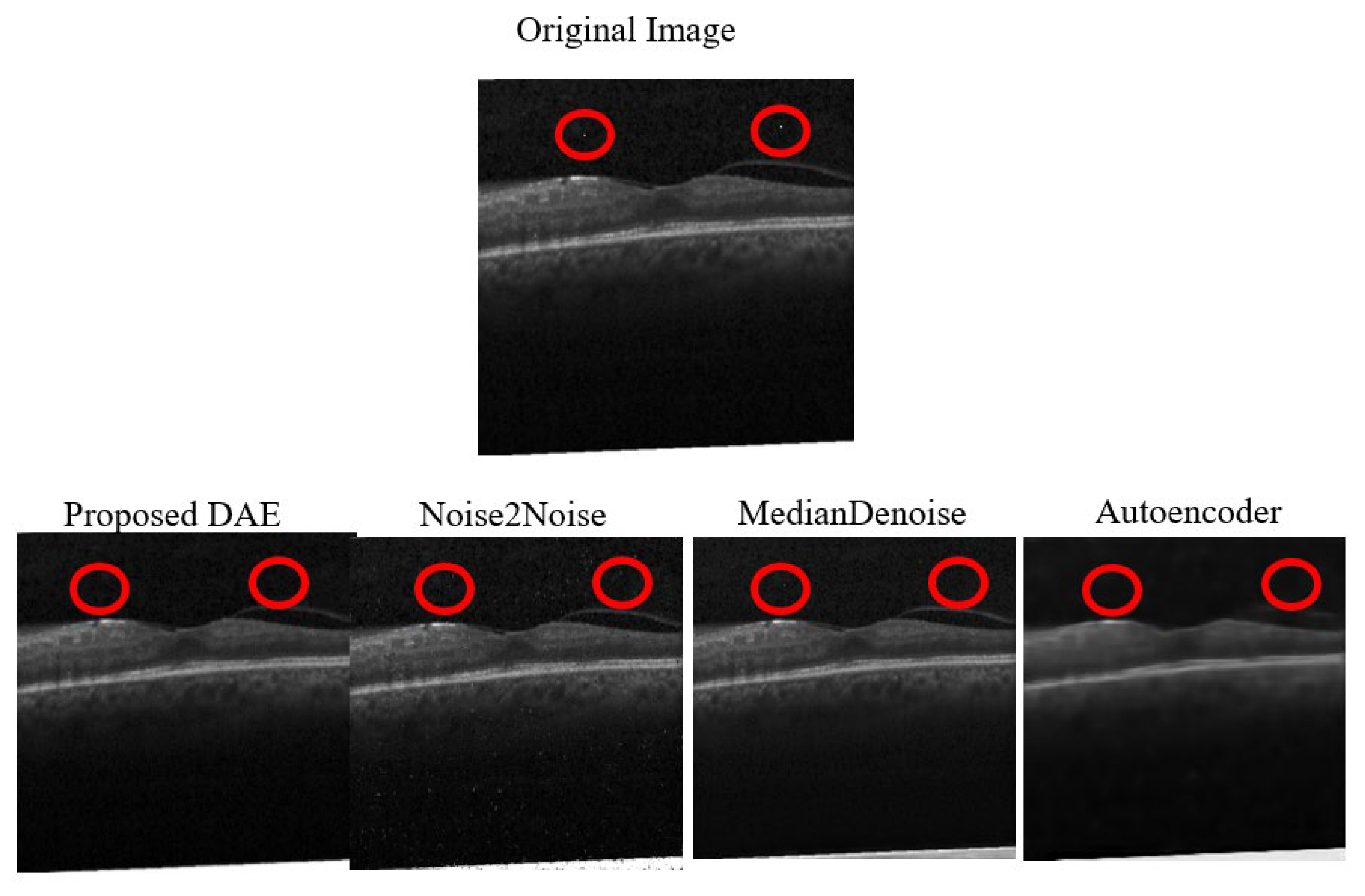
This study is based on applying pixel attacks to images and describing the methods used to restore the attacked images to their original state. The different techniques and theories used in the experiments are described below.

3.1.1. Attack Method

(1)

One-Pixel Attack

The original image is assumed to be represented as an n-dimensional array $x = (x_1,x_2,\dots ,x_n)$, and the machine learning model under attack is denoted as f. The confidence level f(x) can be obtained by inputting the original normal image x into the model f, and then, adversarial images can be generated by perturbing the pixels in the image x. The perturbed pixels can be expressed as. The limit of the perturbation is denoted as L. Given that the set of categories in the dataset is $C = (c_1,c_2,\dots ,c_n)$, and the category of the original image is $c_{ori}$, the goal is to transform it into the adversarial category, where $c_{ori}$, $c_{adv}$ $\in$ C. This problem can be described by the following formula:

$$\underset{{e\left(x\right)}^{\mathrm{*}}}{\max }{f}_{c_{adv}}\left(x+e\left(x\right)\right) subject to {‖e\left(x\right)‖}_0\le L$$

(1)

In the case of a one-pixel attack, since the intention is just to alter a single pixel in the image, the value of L is set to 1, rendering the above objective function as an optimization problem. The most straightforward solution is to make an exhaustive search, which requires trying all combinations composed of the image’s x-coordinates, y-coordinates, and RGB color channels. However, this method requires an enormous amount of time, potentially years, when dealing with large images or images with multiple color channels. For instance, in a 3 × 224 × 224 image, this algorithm must decide the x and y coordinates and the values of the red, green, and blue channels. As each channel has 256 possible combinations and 224 × 224 possible coordinate combinations, 224 × 224 × 256 × 256 × 256 = 841,813,590,016 combinations would need to be applied to generate a single adversarial image. Since it would be inefficient to apply an exhaustive search to this amount of data, differential evolution algorithms are used to generate combinations in these cases.

(2)

Differential Evolution

Differential Evolution (DE) [12] is a branch of the Evolution Strategy (ES) [32], which is designed based on the concept of a natural breeding process. The DE process used in this study is as follows: Initial population, mutation, crossover, selection, termination, and fitness score.

3.1.2. Denoising Model

Different denoising models and combinations will be used in this study to successfully denoise medical images that have been subjected to single pixel attacks, and to compare and analyze the restoration results. Pixel restoration primarily follows the method outlined by Senapati et al. [9], with adjustments made to the model architecture and experimental settings. Three other existing denoising models will also be used for comparison. Image optimization will refer to the approach used by Zhang et al. [22] to more effectively remove noise points from images.

There are several methods to add noise to images, such as salt-and-pepper noise, Gaussian noise, Poisson noise, etc. Among them, random-valued impulsive noise preserves the colors of some pixels and replaces others with random values obtained from a range ${\left[\mathrm{0,1}\right]}^3$ of normalized pixel values cross the RGB channels, rather than replacing them with pure white or black. Each pixel has a probability p of being replaced and a probability 1–p of retaining its original color. Random-valued impulsive noise, compared to Gaussian noise, is a close approximation of the alterations made by single pixel attacks. The different denoising models trained in this study utilize this method of noise addition for denoising purposes. The denoising model architectures used in the study will be introduced separately below, along with their principles.

In the first approach, based on the Noise framework, the authors addressed the single-pixel attack data. Since the noise from these attacks is minimal (a single manipulated pixel), the authors used images with a consistent 10% noise level as both the input and target for model training. For the second, a CNN model incorporating an intermediate layer, we adopted the strategy of Liang et al. [23].

Training images were generated by adding random impulse noise with a noise level incremented by 10% across the range of 10% to 90%, thereby creating a diverse set of noisy inputs. The objective of this training was to optimize the weights for mapping noisy inputs to their clean counterparts. To accommodate the mix of color and grayscale images in the dataset, the number of input layer channels was tailored to the color type of the input image. Both models utilized the Adam optimizer, with training conducted over 100 epochs and a fixed batch size of 16.

(1)

Autoencoder

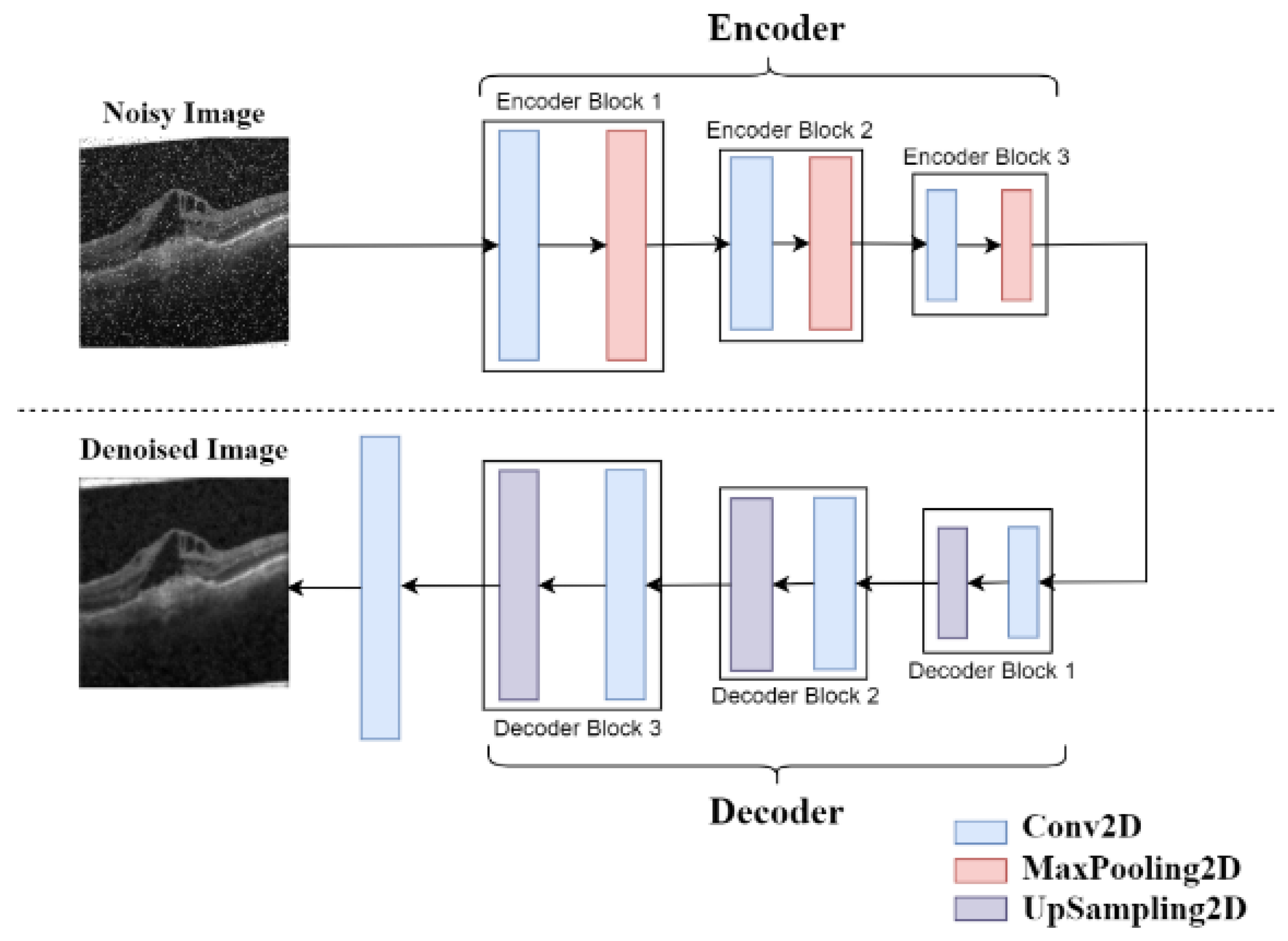
The relatively shallow and straightforward denoising model architecture used by Senapati et al. [9] is shown in Figure 1. Similarly, the decoder part only consisted of three convolutional layers, followed by up-sampling, and finally, an additional convolutional layer was added to reconstruct the image. The details of the single-channel model are presented in

Table 1. Overview of the Autoencoder Single-Channel Layer Outputs and Parameters.

Layer	Layer Type	Output Dimension	Parameters
1	Input	(224, 224, 1)	0
2	Convolution 2-D	(224, 224, 32)	320
3	MaxPooling 2-D	(112, 112, 32)	0
4	Convolution 2-D	(112, 112,8)	2312
5	MaxPooling 2-D	(56, 56, 8)	0
6	Convolution 2-D	(56, 56, 8)	584
7	MaxPooling 2-D	(28, 28, 8)	0
8	Convolution 2-D	(28, 28, 8)	584
9	UpSampling 2-D	(56, 56, 8)	0
10	Convolution 2-D	(56, 56, 8)	584
11	UpSampling 2-D	(112, 112, 8)	0
12	Convolution 2-D	(112, 112, 32)	2336
13	UpSampling 2-D	(224, 224, 32)	0
14	Convolution 2-D	(224, 224, 1)	289
Total Parameters			7009
Trainable Parameters			7009
Non-Trainable Parameters			0

, while those of the RGB three-channel model are shown in

Table 2. Overview of the Autoencoder RGB Channel Layer Outputs and Parameters.

Layer	Layer Type	Output Dimension	Parameters
1	Input	(224, 224, 3)	0
2	Convolution 2-D	(224, 224, 32)	896
3	MaxPooling 2-D	(112, 112, 32)	0
4	Convolution 2-D	(112, 112,8)	2312
5	MaxPooling 2-D	(56, 56, 8)	0
6	Convolution 2-D	(56, 56, 8)	584
7	MaxPooling 2-D	(28, 28, 8)	0
8	Convolution 2-D	(28, 28, 8)	584
9	UpSampling 2-D	(56, 56, 8)	0
10	Convolution 2-D	(56, 56, 8)	584
11	UpSampling 2-D	(112, 112, 8)	0
12	Convolution 2-D	(112, 112, 32)	2336
13	UpSampling 2-D	(224, 224, 32)	0
14	Convolution 2-D	(224, 224, 3)	867
Total Parameters			8163
Trainable Parameters			8163
Non-Trainable Parameters			0

.

(1.1)

Method Validation and Optimization

Experiments were conducted in this study using the AbdomenCT dataset from the Kaggle Medical MNIST, following the experimental set-up by Senapati et al. [9] to validate the original model’s accuracy. The model architecture continued to be modified based on the results of each training session, which led to improved Peak Signal-to-Noise Ratio (PSNR) values. The original dataset image, results of the original study, the experimental results that validated the original model, and the results after optimizing the model are shown from left to right in Figure 2. Meanwhile, the results of denoising from the original study, the validation experiment, and the optimized model are listed in sequence in

Table 3. Validation and Denoising Results of the Optimized Model.

	Paper	Test	Proposed DAE
PSNR	23.91	24.01	30.86
SSIM	0.93	0.92	0.94

.

(2)

Denoising Autoencoder (DAE)

This model refers to the one proposed by Senapati et al. [9] and adjusts the architecture of the original model. An autoencoder is a neural network model primarily used for unsupervised learning and feature learning. Its core concept entails encoding and decoding input data to learn a compressed representation of it while preserving important information. The denoising autoencoder (DAE) used in this study is a variant of autoencoders that are specifically designed to handle noisy data. Unlike traditional autoencoders, the primary goal of DAEs is to restore original noise-free images by learning from noisy input images. They are widely applied to real-world image processing tasks due to their ability to adapt and automatically learn the features of diverse data.

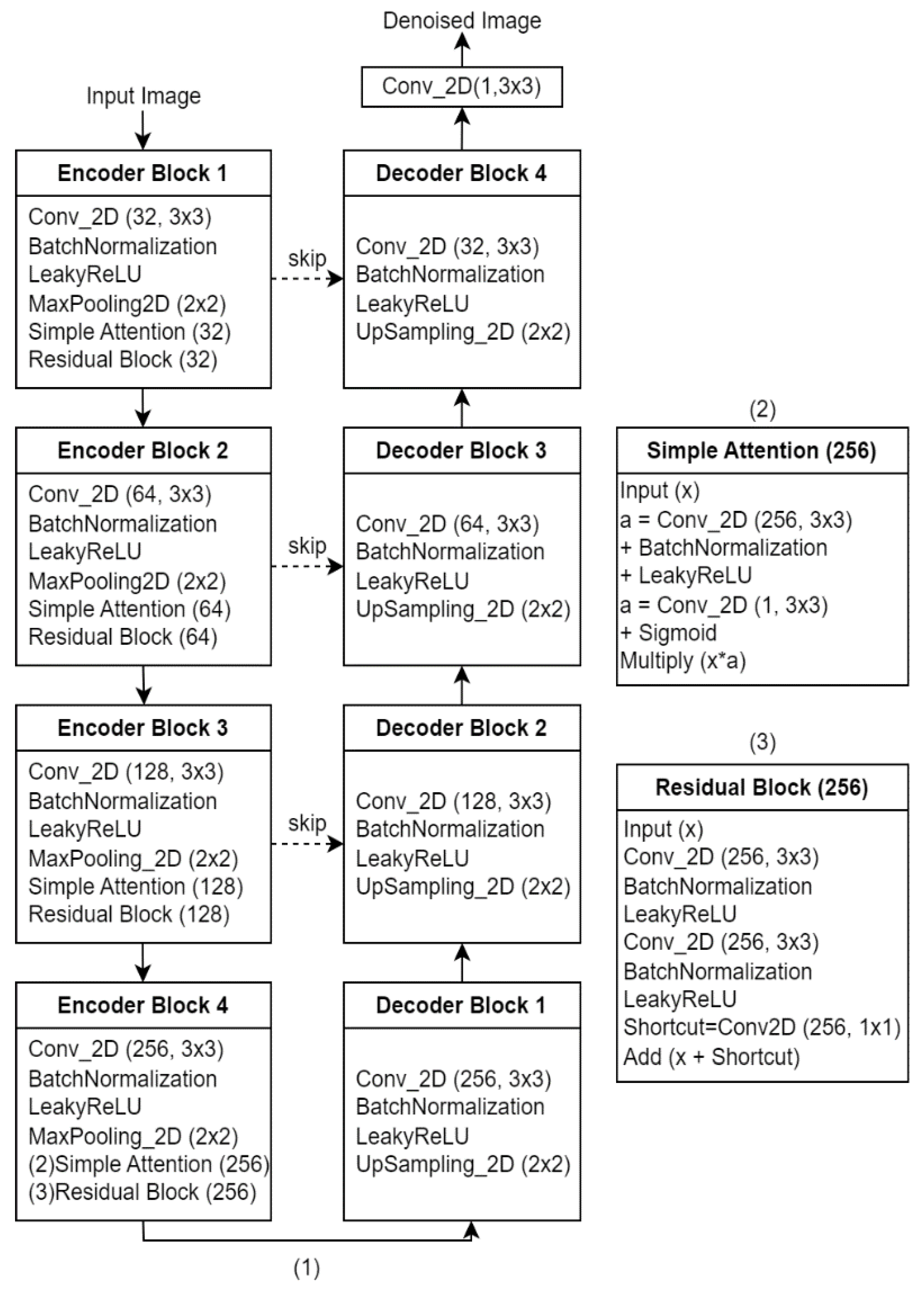
Due to there being considerable room for improvement in the architecture of the original model, sequential adjustments were made to enhance the reconstructed image’s quality and denoising effect. These adjustments were tested using the same Kaggle Abdomen CT public dataset that was used in the original paper, training 10,000 images and testing 2000 images to obtain the average experimental results. The experimental results of the sequential improvements made to the original model architecture are presented in

Table 4. Average Denoising Results of the Model with Sequentially Added Modules.

Model	PSNR	SSIM	MSE	GMSD	FSIM
Original [9]	29.46	0.92	0.0012	0.26	0.13
√	30.65	0.94	0.0009	0.24	0.24
√+★	36.25	0.98	0.0002	0.14	0.36
√+★+▲	36.97	0.98	0.0002	0.15	0.34
√+★+▲+●	37.48	0.99	0.0002	0.13	0.40
Proposed(√+★+▲+●+♦)	40.42	0.99	0.0001	0.1	0.42

Notes: √: increase depth and number of convolutional kernels; ★: Batch Normalization + LeakyReLU; ▲: Simple Attention Layer; ●: Residual Block; ♦: Skip Connection.

, which √ indicates increased depth and number of convolutional kernels, ★ denotes the use of Batch Normalization and LeakyReLU activation, ▲ represents the addition of attention layers, ● signifies residual blocks, and ♦ indicates skip connections. As shown in the table, each module addition resulted in improved experimental outcomes, thereby demonstrating the model’s feasibility.

Additionally, the depth of a model can have a significant impact on its ability to capture the features of an image. However, a model that is too deep may suffer from overfitting, which means that its performance in this study was evaluated to determine if the depth was an issue by reducing and increasing the number of layers in both the encoder and decoder. As in the original paper, the Kaggle Abdomen CT public dataset was used for the test, with 10,000 images for training and 2000 images for testing. The average denoising results for each depth are shown in

Table 5. Average Denoising Results at Different Depths of the Research Model.

Model	PSNR	SSIM	MSE	GMSD	FSIM
3 Layer	38.16	0.99	0.0002	0.13	0.39
Proposed (4 Layer)	40.42	0.99	0.0001	0.1	0.42
5 Layer	37.25	0.99	0.0002	0.13	0.38

. The experimental results indicate that the model achieves a better denoising performance at the current depth by effectively capturing the features of the image without encountering an overfitting issue, thereby validating the appropriateness of the model design at this depth.

The simple architecture of the original model is shown in Figure 3, while the improved model’s simplified architecture is depicted in Figure 4. A detailed schematic of the model can be seen in Figure 4 and Figure 5.

In contrast, non-trainable parameters are primarily found in Batch Normalization layers. As these mean and variance parameters are solely used to normalize the data and otherwise remain fixed throughout this process, with no incremental updates, they are classified as non-trainable. The performance of the model is primarily improved by learning and adjusting the trainable parameters, while the non-trainable parameters are used to normalize the data, which helps to maintain the model’s stability.

(2.1)

Encoder

In the encoding phase, the model transforms the input into a latent representation that captures the primary features of the input image. The noise filter function in the encoder enables the model to perform effectively when dealing with noisy images. The Denoising Autoencoder (DAE) learns to effectively filter out noise while preserving important image information when trained on noisy images, which enhances the model’s robustness and improves its ability to remove unnecessary noise during image reconstruction. 10% random impulse noise is added to images before training to enable the model to perform denoising training. Since the size of the attacked image is 224 × 224, the encoder input size is also set to 224 × 224. A detailed explanation will be provided in this study of the optimizations made to the original model [9] and how these improvements are reflected in the experimental results. These optimizations include increasing the depth of the model and the number of convolutional kernels, using Batch Normalization and LeakyReLU activation functions, introducing a Simple Attention Layer, embedding residual blocks, and adding Skip Connections.

In Figure 4, √ denotes an increase in the model’s depth and the number of convolutional kernels. The ★ symbol indicates the addition of Batch Normalization and LeakyReLU activation functions in the model, significantly improving its training stability and expressiveness. The ▲ symbol represents the introduction of the Simple Attention Layer into the model, which aims to enable the model to focus adaptively on important parts of the input. The ● symbol indicates the embedding of residual blocks, which can also enhance the performance of deep models. Residual blocks introduce skip connections that directly add the input to the output, thereby addressing common issues in deep models, such as vanishing and exploding gradients. Finally, the ♦ symbol represents the addition of Skip Connections, further enhancing the flow of information within the model.

These encoder optimizations enable the model to identify and extract useful information more effectively during the initial feature extraction phase.

(2.2)

Decoder

In the decoding phase, the model maps the latent representation back to the original input to reconstruct the original data. The decoder’s primary goal is feature restoration. By learning to effectively reverse the latent representation generated by the encoder and reconstruct it into the original image, the decoder can rebuild important features from the input image.

This study used a mirrored convolutional layer configuration for the decoder, which was opposite to that of the encoder. The Denoising Autoencoder (DAE) used this mirrored design to take advantage of data symmetry, which improved its learning efficiency and enabled it to more effectively capture the image’s features.

Optimizations to the decoder in the new denoising model compared to the original model described in the paper are explained in detail in the next sections, along with the contribution they made to the improved experimental results.

Due to the mirrored design of the encoder and decoder, the decoder also has a depth of four layers, as indicated by the √ symbol. A deeper decoder can reconstruct images better because the deeper layers can progressively recover detailed information. The network can learn more comprehensive reconstruction features as the depth of the model increases, leading to an improved performance in restoring image details. Additionally, increasing the number of convolutional kernels enhances the model’s capability to capture a richer set of features.

Furthermore, both the encoder and decoder use the Batch Normalization and LeakyReLU activation functions. Batch Normalization helps the model to achieve better reconstruction results, while LeakyReLU facilitates learning in the negative value region, which enhances the model’s expressiveness and stability during decoding, thereby improving its ability to reconstruct features effectively.

In summary, these optimizations ensure that the decoder can more effectively restore the original image features, enhancing denoising and better restoration quality.

(3)

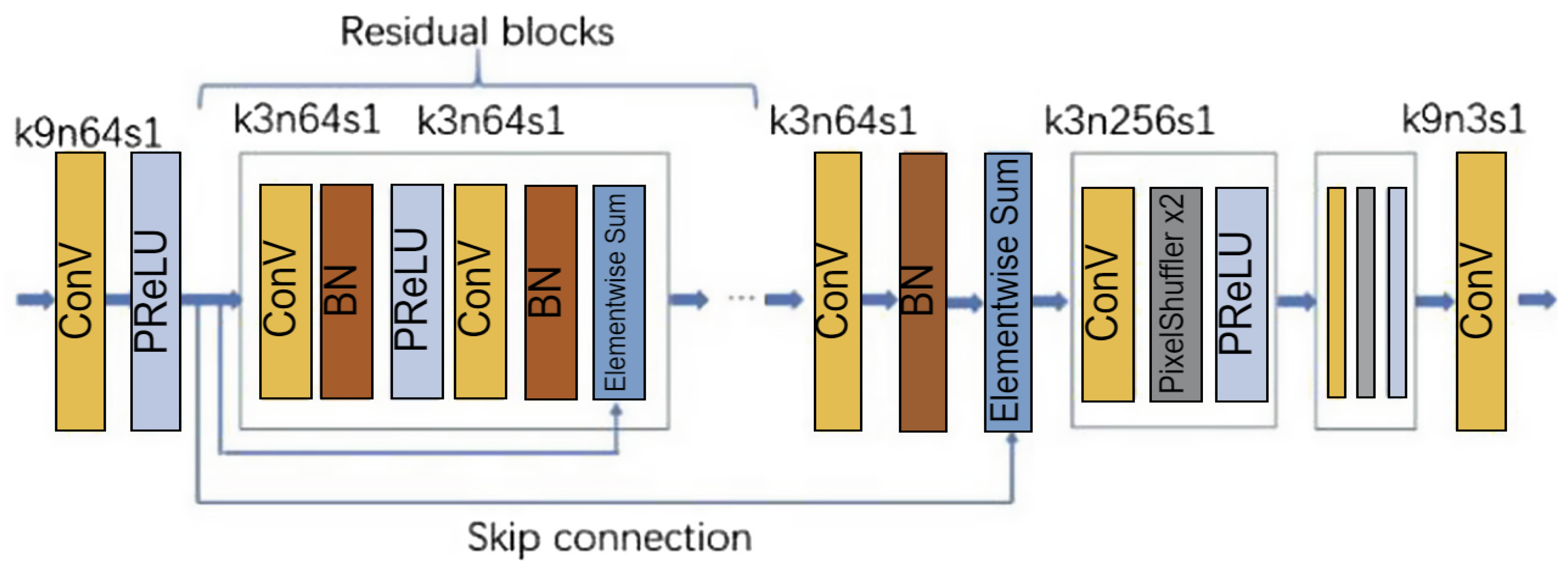
SRResNet Based on Noise2Noise Framework

Chen et al. [5] used the Noise2Noise framework for denoising, disregarding the need to obtain many clean images and making it unnecessary to train with many noisy images and corresponding clean images. The original data only requires some original images to which noise is added to generate multiple noisy images to serve as input images and target images for training the deep learning model. When using the Noise2Noise framework, it is necessary to choose an appropriate deep neural network structure, appropriate noise type, and loss function to defend an image against a one-pixel attack. SRResNet (as shown in Figure 6) is used as the deep learning structure. This generator network in SRGAN is mainly used for image super-resolution (SR) tasks. It improves the image quality by learning the mapping relationship between high-resolution and low-resolution images. This model is mainly constructed of 16 residual blocks. The network structure does not restrict the size of the input image, and the size of the input and output images is the same. This network model can remove Gaussian noise, impulsive noise, Poisson noise, and text. It is suitable for the defense models of many different types of source data because it constructs safe applications. The loss function used here is the annealed version of the L₀ loss function, which is based on the following formula;

$${\left(\left|f_{\theta }\left(\hat{x}\right)-\hat{y}\right|+\epsilon \right)}^{\gamma }$$

(2)

where f represents the neural network model, =10^–8, and ^γ will be annealed linearly from 2 to 0 during training. In this case, the added random noise has the characteristic of zero expectation, and the loss function will not learn the characteristic of the noise. Therefore, the same effect for training will be achieved using noisy and non-noisy images. As a result, the model parameters obtained will be very close to those obtained by training with clean images, which enables the model to be trained to efficiently denoised images without requiring pairs of noisy and corresponding clean images.

(4)

CNN with a Median Layer

Liang et al. [23] proposed this denoising model, which was primarily designed to remove salt-and-pepper noise, a type of impulsive noise. The denoising effect is achieved by combining the deep neural network model with a median filter, a conventional nonlinear filter, which is particularly effective in removing impulsive noise by replacing the center pixel with the median value of a given window. The so-called median layer is defined as the application of the median filter with a moving window method on each feature channel. For example, an RGB color input image corresponds to three feature channels, and there may be multiple sets of features after convolution. Patches of a specified size (e.g., 3 × 3 or 5 × 5) need to be extracted from each channel pixel to apply the filter, and the median of the elements in each patch forms a new sequence. The median layer is applied to each feature channel and then combined to create a new set of features. If the convolution generates 64 feature channels, the median layer will be applied 64 times.

As shown in Figure 7, this is a fully convolutional neural network (FCNN) in which the input data size is not restricted. Its architecture starts with two consecutive median layers, followed by a series of residual blocks and interleaved median layers, while the last part only consists of residual blocks between which median layers are inserted in the first half of the sequence. Each convolutional layer generates 64 features, and the residual blocks are designed as residual connections spanning two layers of 64 feature convolutions, followed by batch normalization layers and rectified linear unit (ReLU) activation functions, as shown in Figure 7b. This model utilizes the simplest L₂ as the objective loss function, and the loss can be simply defined as the mean squared error between the estimated image and the ground truth image. This is because minimizing the mean squared error is directly related to increasing the denoising performance metric, peak signal-to-noise ratio (PSNR).

3.2. Research Design

The experiments of this study were conducted using the medMNIST dataset, a comprehensive collection of diverse medical images. This dataset includes dermatoscopic, hematoxylin & eosin-stained, optical coherence tomography (OCT) scans, and X-rays, each with its own original image size. The medMNIST dataset is highly versatile, supporting both single-label and multi-label classification tasks while also featuring a mix of color and grayscale images. The details of the software implemented in the research are listed in the Appendix A.

The research process can be divided into three stages and is simplified, as shown in Figure 8. The experiment mainly consists of the training stage, the attack stage, and image denoising. Initially, classification and denoising models are trained on different datasets, and single-pixel attacks generate adversarial images. Finally, the “successfully attacked adversarial images,” which are those that failed the classification post-attack, are used as test images. They are then input into the trained denoising models for denoising, and the results of various different models are compared and analyzed. The datasets and experimental details are introduced in the next sections.

3.2.1. Dataset

The experiments were conducted using publicly available medical images from the four original datasets of medMNIST: Derma, Pathology, OCT, and Chest as shown in

Table 6. Overview Information of Dataset.

Name	Number of Data	Number of Class	Original Size of Image	Type of Dataset	Color Information	Type of Image
Derma	10,015	7	600 × 450	Multi-class	Color	Dermatoscopic
Pathology	100,000	10	224 × 224	Multi-class	Color	Hematoxylin & eosin-stained
OCT	109,309	4	(1, 3) × (384~1, 536) × (277~512)	Multi-class	Grayscale	Optical Coherence Tomography
Chest	112,120	14	1024 × 1024	Binary-class multi-label	Grayscale	X-ray

.

(1)

Derma

The Derma dataset [33] consists of multi-class pigmented skin lesions, which are common pigmentary skin disorders. It contains 10,015 color images with dimensions of 3 × 600 × 450 captured by a dermatoscope. An overview of the class data distribution in the dataset is provided in

Table 7. Overview of Derma Dataset.

Class	Disease Type	Count	Percentage
Actinic keratoses and intraepithelial carcinoma	Disease	327	3.27%
Basal cell carcinoma	Disease	514	5.13%
Benign keratosis-like lesions	Normal	1099	10.97%
Dermatofibroma	Normal	115	1.15%
Melanoma	Disease	1113	11.11%
Melanocytic nevi	Normal	6705	66.95%
Vascular lesions	Disease	142	1.42%

, with class names representing the different types of skin lesions displayed in the “Class” column. The class attributes are described in the “Disease Type” column, where “Normal” indicates non-pathological symptoms that do not require treatment, and “Disease” indicates potentially harmful symptoms that do require medical attention. The total number of original data samples in each class is indicated in the “Count” column, and the proportion of each class in the entire dataset is represented in the “Percentage” column.

(2)

Pathology

The Pathology dataset is the original size dataset of pathMNIST, which is described in a previous study [34] as consisting of color images with dimensions of 3 × 224 × 224. The NCT-CRC-HE-100K dataset contains 100,000 images with the same class labels as pathMNIST. An overview of this dataset is provided in

Table 8. Overview of Pathology Dataset.

Class	Disease Type	Count	Percentage
Adipose	Normal	10,407	10.08%
Background	Normal	10,566	10.60%
Debris	Normal	11,512	11.55%
Lymphocytes	Normal	11,557	11.60%
Mucus	Normal	8896	8.93%
Smooth Muscle	Normal	13,536	13.58%
Normal Colon Mucosa	Normal	8763	8.79%
Cancer-associated Stroma	Disease	10,446	10.48%
Colorectal Adenocarcinoma Epithelium	Disease	14,317	14.37%

.

(3)

OCT

The OCT (Optical Coherence Tomography) dataset consists of grayscale images of retinal diseases obtained from optical coherence tomography scans. This multi-class dataset is derived from a previous study [35]. It comprises 109,309 images, the original size of which ranged from (1, 3) × (3841,536) × (277,512), but they were all converted to grayscale for these experiments. An overview of the dataset is provided in

Table 9. Overview of OCT Dataset.

Class	Disease Type	Count	Percentage
Normal	Normal	51,390	47.01%
Choroidal neovascularization	Disease	37,455	34.27%
Diabetic macular edema	Disease	11,598	10.61%
Drusen	Disease	8866	8.11%

.

(4)

Chest

The Chest dataset is a binary-class multi-label dataset comprising 112,120 frontal-view X-ray chest grayscale images in 14 disease categories, derived from the NIH-ChestXray14 dataset [36]. The original size of the images was 1 × 1024 × 1024 pixels. Since there are 14 labels, each of which is represented by either 0 or 1, there are 2¹⁴ = 16,384 possible category combinations. This would require a substantial amount of time to conduct 1,638,400 experiments on the Chest dataset, which would be impractical.

However, the dataset only consists of 247 distinctive combinations, most containing fewer than 100 images and some even fewer than 10. Due to the limited availability of training images, the five single-label category combinations with the highest amount of data were selected for the subsequent defense experiments. This selection ensured that the model could correctly classify all categories of images. The category proportion of the five single-label categories used in this study is listed in

Table 10. Overview Information of Chest Dataset used in This Research.

Class	Disease Type	Original	Percentage
Normal	Normal	60,361	53.84%
Atelectasis	Disease	4215	3.76%
Effusion	Disease	3955	3.53%
Infiltration	Disease	9547	8.51%
Nodule	Disease	2705	2.41%

.

3.2.2. Image Classification

The classification models were first trained on four different medical imaging datasets to evaluate their accuracy. All the datasets, apart from the Chest dataset, were divided into training and testing sets in an 8:2 ratio. The three datasets were handled with the images partitioned into 70% for training, 10% for validation, and the final 20% reserved for control and comparison purposes, ensuring this reserved portion was not included in the training process. However, the Chest dataset had multiple labels, some of which only contained one image, which made it impossible to divide them into separate training and testing sets. Additionally, the “Normal” category was excluded from the multi-label training because all the labels in this category were zero, which could potentially mislead the model to learn in the wrong direction. Meanwhile, the “Normal” class accounted for the largest proportion of the dataset, meaning up to 94% accuracy could be achieved by predicting the cases as “Normal”, but the images from the other categories would not be classified accurately. Therefore, this class was excluded from the training experiments to ensure accurate results.

With regard to the models, convolutional neural networks (CNNs) based on convolutional operations are most commonly used for training image classification tasks. The ResNet [37] series of models has been widely adopted due to their characteristic of deep residual learning, which ensures high performance and good generalization across various visual tasks. Chen et al. [5] and Liang et al. [23] have also utilized these models for image classification tasks. The standard ResNet [38] models are ResNet18, ResNet34, ResNet50, and the largest, ResNet152. ResNet50, with a certain depth, was chosen as the classification model in this research due to its excellent performance in image classification tasks and its deeper architecture, which enables the capture of the more intricate features and patterns in medical images.

4. Experiments and Results

4.1. Experimental Set-Up

4.1.1. Experimental Equipment

Two computers were used to conduct the experiments in this study. Computers A and B were laboratory equipment. The hardware specifications are provided in

Table 11. Hardware Specifications.

Hardware	Component	Information
Computer A	CPU	11th Gen Intel(R) Core(TM) i7-11700KF @ 3.60 GHz
	GPU	NVIDIA GeForce RTX 3060
	RAM	16 GB
Computer B	CPU	11th Gen Intel(R) Core(TM) i7-11700K @ 3.60 GHz
	GPU	NVIDIA GeForce RTX 3090
	RAM	32 GB

.

4.1.2. Parameter Setting

(1)

Classification Model

ResNet50 [37] was the image classification model used in this study, together with a stochastic gradient descent (SGD) optimizer with a learning rate of 0.001 and momentum of 0.9. Each model was trained for 100 epochs with a batch size of 64. Training could be stopped upon meeting the early stopping criteria, which included training accuracy of over 95% and a testing accuracy above 90%.

(2)

One-Pixel Attack

In this experiment, the untrained test sets from four different datasets were first input into the classification models to obtain correctly classified images. These images are then subjected to single-pixel attacks to generate adversarial images, including successful attacks (pixels are altered and misclassified) and unsuccessful attacks. The resulting images were resized to 224 × 224, and only “successfully attacked” adversarial images were used in the subsequent experiments.

All the one-pixel attacks in this study were non-targeted. No crossover was performed during the Differential Evolution (DE) process, and the mutant factor was set at 0.5. The population size was set at 100, and the maximum iteration limit was 100. The process could be terminated if all adversarial images have been generated.

(3)

Denoising Model

Successfully attacked medical images (where pixels had been altered and misclassified) were subjected to image denoising to reconstruct them to closely resemble the original images. Four different denoising models were trained in this study by adding noise to the original images. The successfully attacked images were used as test images to see if the altered pixels could be successfully restored. The results of denoising each model were then analyzed and compared.

Each denoising model was trained on all of the datasets. Since a single pixel attack only alters one pixel per image, resulting in a very low noise ratio, the models used images with a noise level of 10% as both input and test images. The aim of this approach was to train the models to learn the weights of converting noisy input images into clean ones. Different input layer channels were used since the datasets included both grayscale and color images, but all four models used Adam as the optimizer.

Five different image metrics were used to evaluate the similarity between the original and reconstructed images to quantify the denoising effectiveness of the different models in reconstructing images in this study. Each of these metrics is described below.

(1) The Peak Signal-to-Noise Ratio (PSNR) is a measure of image quality used to evaluate the degree of distortion before and after image reconstruction. A higher value indicates a higher similarity between the reconstructed image and the original image, signifying better quality.

$$PSNR=10\cdot {log}_{10}\left({\displaystyle \frac{M{AX}^2}{MSE}}\right)$$

(3)

$MAX$ is the maximum possible pixel value of the image. $MSE$ is the Mean Squared Error between the original and reconstructed images.

(2) The Structural Similarity Index (SSIM) is a metric used to measure the structural similarity of two images by considering the differences in luminance, contrast, and structure to provide a more objective evaluation of the image quality. The value ranges from 0 to 1, where a value closer to 0 indicates less similarity and a value closer to 1 indicates greater similarity.

$$SSIM\left(x,y\right)={\displaystyle \frac{\left(2{\mu }_x{\mu }_y+C_1\right)\left(2{\sigma }_{xy}+C_2\right)}{\left({\mu }_x^2{+\mu }_y^2+C_1\right)\left({\sigma }_x^2+{\sigma }_y^2+C_2\right)}}$$

(4)

$x$ and$y$are the original and reconstructed images, ${\mu }_x^2$ and ${ \mu }_y^2$ are the average luminance values of images $x$ and $y$, ${\sigma }_x^2$ and ${\sigma }_y^2$ are the variances of images$x$and$y$,${\sigma }_{xy}$ is the covariance between images$x$and$y$, $C_1$ and $C_2$ are constants that stabilize the division when the denominator is small.

(3) The Mean Squared Error (MSE) is a metric used to evaluate the difference between two images by calculating the average of the squared differences between corresponding pixels in the reconstructed image and those in the original image. A smaller value indicates a greater similarity between the two images.

$$MSE={\displaystyle \frac{1}{n}}\sum _{i=1}^n{(y_i-{\widehat{y}}_i)}^2$$

(5)

$n$ represents the number of images, $y_i$ represents the true value of the$i$-th image, and ${\widehat{y}}_i$ represents the predicted value of the $i$-th image.

(4) The Gradient Magnitude Similarity Deviation (GMSD) is a metric used to measure the quality of the image by comparing the different gradients of the reconstructed and the original images. The different quality of the images is assessed based on these different gradients. The value ranges from 0 to 1, with a smaller value indicating less distortion.

$$GMSD=\sqrt{{\displaystyle \frac{1}{N}}{\sum }_{i=1}^N{\left(GMS\left(i\right)-GMSM\right)}^2}$$

(6)

$GMS$ is the Average gradient magnitude for each image $i$, $GMSM$ is the global average of $GMS$ across all images. For more details, please refer to [38].

(5) The Feature Similarity Index (FSIM) is a means of evaluating the similarity of the features of the reconstructed and original images. Its value ranges from 0 to 1, with a value closer to 0 indicating less similarity and a value closer to 1 indicating more similarity.

$$FSIM={\displaystyle \frac{{\sum }_{x\in \Omega }{S}_L\left(x\right)\cdot {PC}_m\left(x\right)}{{\sum }_{x\in \Omega }{PC}_m\left(x\right)}}$$

(7)

Here, ${\sum }_{x\in \Omega }{S}_L\left(x\right)$ denotes the sum of local feature similarities $S_L\left(x\right)$ at all pixels $x$ within the region Ω, and ${PC}_m\left(x\right)$ represents the pixel contrast at position $x$. For more details, please refer to [39].

4.2. Pixel Attack of Attacked ResNet50 and Its Denoising Results

4.2.1. Image Classification of ResNet50

The final accuracy results and the number of correctly classified images obtained from training the ResNet50 classification model on four medical imaging datasets are illustrated in

Table 12. Classification Results of ResNet50.

Dataset	Training Accuracy	Test Accuracy	Accurate Images
Derma	99.91%	83.02%	1669
Pathology	98.16%	95.56%	19,111
OCT	96.51%	96.17%	21,024
Chest	95.22%	90.30%	5508

. “Training Accuracy” refers to the accuracy of the training set, “Test Accuracy” represents the accuracy of the test set, and “Accurate Images” indicates the number of correctly classified images in the test set. It can be observed that the classification models achieved good training set accuracy for all datasets. In terms of the accuracy of the test sets, all the datasets apart from Derma, exceeded 90% and demonstrated a certain level of classification accuracy. The Derma dataset’s slightly lower test set accuracy was possibly due to overfitting during the training process. However, it still exhibited a reasonable level of accuracy compared to previous results. Therefore, this classification model was used to determine the classification results in subsequent experiments.

The predictive capabilities of the classification models for each dataset are presented in

Table 13. Prediction Capability of the ResNet50 Derma Classification Model.

Class	Precision	Recall	F1 Score
Actinic keratoses and intraepithelial carcinoma	59%	57%	57%
Basal cell carcinoma	67%	77%	71%
Benign keratosis-like lesions	68%	63%	65%
Dermatofibroma	77%	43%	56%
Melanoma	64%	51%	57%
Melanocytic nevi	90%	94%	92%
Vascular lesions	85%	79%	81%

,

Table 14. Prediction Capability of the ResNet50 Pathology Classification Model.

Class	Precision	Recall	F1 Score
Adipose	100%	99%	99%
Background	100%	100%	100%
Debris	99%	96%	98%
Lymphocytes	100%	100%	100%
Mucus	90%	100%	95%
Smooth Muscle	84%	99%	91%
Normal Colon Mucosa	99%	96%	98%
Cancer-associated Stroma	98%	70%	81%
Colorectal Adenocarcinoma Epithelium	97%	99%	98%

,

Table 15. Prediction Capability of the ResNet50 OCT Classification Model.

Class	Precision	Recall	F1 Score
Normal	96%	98%	97%
Choroidal neovascularization	96%	92%	94%
Diabetic macular edema	86%	83%	85%
Drusen	98%	98%	98%

and

Table 16. Prediction Capability of the ResNet50 Chest Classification Model.

Class	Precision	Recall	F1 Score
Atelectasis	22%	23%	22%
Effusion	37%	38%	38%
Infiltration	28%	35%	31%
Nodule	19%	1%	3%

. The precision and recall for each class are listed to provide a more detailed insight into each model’s classification performance. The following formulas were used for the Recall, Precision, and F1 Scores;

$$Recall={\displaystyle \frac{TP}{TP+FN}}$$

(8)

$$Presision={\displaystyle \frac{TP}{TP+FP}}$$

(9)

$$F1 Score=2\times {\displaystyle \frac{Precision\times Recall}{Precision+Recall}}$$

(10)

Here, $TP$ (True Positives) represents the number of images that are positive and were correctly detected as positive, while $FN$ (False Negatives) represents the number of positive images but were incorrectly detected as negative, and $FP$ (False Positives) represents the number of images that are negative, but were incorrectly detected as positive.

Based on the table, the model performed well in classifying the different categories in the OCT and Pathology datasets. However, in the Chest dataset, due to significant differences in class proportions, the model’s predictive performance remained suboptimal despite excluding the Normal class, which is most likely to mislead the model, and training only on the four most populous “single-label” classes. This may be attributed to the high complexity and imbalance inherent in this binary multi-label dataset, which makes it difficult for the model to predict certain classes accurately. This issue could be rectified by future research adopting the approach used in [40], in which autoencoders were combined with One-Class SVM, which effectively addressed the imbalance problem and could improve the model’s accuracy. Also, the relatively poor classification of Derma may have been due to the smaller number of images in the dataset.

4.2.2. Derma of ResNet50

• One-Pixel Attacks

The four medical imaging datasets were then subjected to a one-pixel attack. The test sets mentioned earlier, which were not being used to train classification models, were put into the models first for classification. The correctly classified images were then subjected to a one-pixel attack. Based on the results of these attacks presented in the first table below, “Test Count” represents the number of test set images correctly classified. The “Success Count” represents the number of successfully attacked images, and the “Success Rate” represents the success rate of each attack category.

The results of attacks on the Derma dataset presented in

Table 17. Results of Derma One-Pixel Attacks.

Class	Disease Type	Test Count	Success Count	Success Rate
Actinic keratoses and intraepithelial carcinoma	Disease	37	12	32.43%
Basal cell carcinoma	Disease	79	14	17.72%
Benign keratosis-like lesions	Normal	139	35	25.18%
Dermatofibroma	Normal	10	3	30.00%
Melanoma	Disease	114	34	29.82%
Melanocytic nevi	Normal	1268	78	6.15%
Vascular lesions	Disease	22	2	9.09%

below show that 178 of the total 1669 images had been successfully attacked, resulting in an overall attack success rate of 10.67%. When calculating the success rate for each category separately, the average attack success rate for the entire dataset was 21.48%. This indicates that two categories in the Derma dataset had a successful attack rate of below 10%, implying that these two categories were less susceptible to successful attacks.

The average denoising results of the Derma dataset of each model are shown in

Table 18. Denoising One-Pixel Attack Image Result of Derma.

Model	PSNR	SSIM	MSE	GMSD	FSIM
Proposed DAE	37.60	0.98	0.0002	0.13	0.48
Noise2Noise [5]	32.00	0.60	50.95	0.25	0.24
MedianDenoise [23]	37.52	0.99	0.0002	0	1
Autoencoder [9]	34.89	0.96	0.0004	0.18	0.29

below. The 178 Derma images that were successfully attacked using One-Pixel attacks and the reconstructed images after denoising by each model are, respectively, shown in Figure 9.

It can also be observed from these results that the DAE model proposed in this study has a similar performance to that of the MedianDenoise in most metrics. The images produced by the model are closer in color to the original images, although the MedianDenoise generates brighter images, while Noise2Noise produces denoised images with more noise compared to others. It is also evident when comparing the four images that the features of the images reconstructed by the Autoencoder are much more blurred than those of the original images. As a result, the proposed method regarding detecting one-pixel attacks is better than existing research [8].

2.

Two-Pixel Attacks

In addition to One-Pixel attacks, images subjected to Two-pixel attacks were also attacked and denoised in this study to verify whether the denoising model proposed in this study could successfully restore the pixels that had been altered in a Two-Pixel attack.

The statistical results of the Two-pixel attacks on the Derma dataset are presented in

Table 19. Derma Two-Pixel Attack Results.

Class	Disease Type	Test Count	Success Count	Success Rate
Actinic keratoses and intraepithelial carcinoma	Disease	100	35	35%
Basal cell carcinoma	Disease	100	25	25%
Benign keratosis-like lesions	Normal	100	36	36%
Dermatofibroma	Normal	100	30	30%
Melanoma	Disease	100	36	36%
Melanocytic nevi	Normal	100	7	7%
Vascular lesions	Disease	100	14	14%

, from which it can be seen that 183 of the total 700 images had been successfully attacked and their categories had been altered, resulting in an overall success rate of 26.14%. This is an improvement from the 10.67% success rate of One-Pixel attacks. Examples of successful Two-Pixel attacks on the Derma dataset are provided in Figure 10 below.

The average denoising results for each model in the Derma dataset are shown in

Table 20. Denoising Two-Pixel Attack Image Result of Derma.

Model	PSNR	SSIM	MSE	GMSD	FSIM
Proposed DAE	37.43	0.98	0.0002	0.13	0.49
Noise2Noise [5]	32.00	0.60	50.95	0.25	0.24
MedianDenoise [23]	37.20	0.99	0.0002	0	1
Autoencoder [9]	34.74	0.96	0.0004	0.18	0.30

below. The Derma images that were attacked successfully using a Two-Pixel attack and the images that were reconstructed after being denoised by each model are shown, respectively, in Figure 11.

4.2.3. Pathology of ResNet50

1.

One-Pixel Attacks

The results of the attack for the Pathology dataset are presented in

Table 21. Pathology One-Pixel Attack Results.

Class	Disease Type	Test Count	Success Count	Success Rate
Adipose	Normal	2056	2	0.10%
Background	Normal	2106	3	0.14%
Debris	Normal	2203	19	0.86%
Lymphocytes	Normal	2305	3	0.13%
Mucus	Normal	1772	2	0.11%
Smooth Muscle	Normal	2691	12	0.45%
Normal Colon Mucosa	Normal	1686	17	1.01%
Cancer-associated Stroma	Disease	1453	73	5.02%
Colorectal Adenocarcinoma Epithelium	Disease	2839	8	0.28%

below. 139 of the total 19,111 images were successfully attacked, resulting in an overall success rate of attacks of 0.73%, which is extremely low. When the success rate was calculated separately for each category, the average success rate of attacks for the entire dataset was 0.9%. Among these categories, only “Cancer-associated Stroma” achieved a relatively higher successful attack rate, while the success rates of the remaining categories were slightly below 1%. Examples of a successful One-Pixel attack on the Pathology dataset are shown in Figure 12 below.

2.

Two-Pixel Attacks

The statistical results of the Two-Pixel attacks on the Pathology dataset are presented in

Table 22. Pathology Two-Pixel Attack Results.

Class	Disease Type	Test Count	Success Count	Success Rate
Adipose	Normal	100	1	1%
Background	Normal	100	1	1%
Debris	Normal	100	1	1%
Lymphocytes	Normal	100	1	1%
Mucus	Normal	100	1	1%
Smooth Muscle	Normal	100	2	2%
Normal Colon Mucosa	Normal	100	2	2%
Cancer-associated Stroma	Disease	100	3	3%
Colorectal Adenocarcinoma Epithelium	Disease	100	1	1%

. 13 of the total 900 images were successfully attacked and had their categories altered, resulting in an overall success rate of 1.44%. This was an improvement on the 0.9% success rate of the One-Pixel attacks. Figure 13 below contains some examples of a successful Two-Pixel attack on the Pathology dataset.

The average denoising results for each model on the Pathology dataset are presented in

Table 23. Denoising Two-Pixel Attack Image Result of Pathology.

Model	PSNR	SSIM	MSE	GMSD	FSIM
Proposed DAE	35.48	0.98	0.0004	0.08	0.87
Noise2Noise [5]	29.12	0.86	38.68	0.18	0.74
MedianDenoise [23]	34.32	0.98	0.0008	0.03	1
Autoencoder [9]	23.36	0.69	0.0059	0.26	0.30

below. Images of the Pathology that were successfully subjected to Two-Pixel attacks, together with the reconstructed images after being denoised by each model are, respectively, shown in Figure 14. The red circles indicate the pixels that were altered during the Two-Pixel attacks.

4.2.4. OCT of ResNet50

1.

One-Pixel Attacks

The results of attacks of the OCT dataset are presented in

Table 24. OCT One-Pixel Attack Results.

Class	Disease Type	Test Count	Success Count	Success Rate
Normal	Normal	10,060	5693	56.59%
Choroidal neovascularization	Disease	7361	121	1.64%
Diabetic macular edema	Disease	2124	78	3.67%
Drusen	Disease	1479	321	21.70%

below. 6213 of the total 21,024 images were successfully attacked, resulting in an overall attack success rate of 29.55%. When calculating the success rate separately for each category, the average attack success rate for the entire dataset was 20.9%. The “Normal” category had the highest success rate of all the categories, indicating that it was the category most vulnerable to attack.

The average denoising results for each model on the OCT dataset are shown in

Table 25. Denoising One-Pixel Attack Image Result of OCT.

Model	PSNR	SSIM	MSE	GMSD	FSIM
Proposed DAE	37.62	0.98	0.0002	0.09	0.83
Noise2Noise [5]	32.11	0.89	10.04	0.21	0.77
MedianDenoise [23]	33.33	0.98	0.0008	0.06	0.99
Autoencoder [9]	30.21	0.91	0.001	0.27	0.25

. The images of OCT that were successfully attacked with One-Pixel attacks are, respectively, shown in Figure 15, along with the reconstructed images after being denoised by each model. The red circles indicate the pixels that were altered during the One-Pixel attacks.

2.

Two-Pixel Attacks

The statistical results of the Two-Pixel attacks on the OCT dataset are presented in

Table 26. OCT Two-Pixel Attack Results.

Class	Disease Type	Test Count	Success Count	Success Rate
Normal	Normal	100	81	81%
Choroidal neovascularization	Disease	100	1	1%
Diabetic macular edema	Disease	100	2	2%
Drusen	Disease	100	35	35%

. 119 of the total 400 images were successfully attacked and had their categories altered, resulting in an overall success rate of 29.75%. This was an improvement on the 29.55% success rate of One-Pixel attacks.

The average denoising results for each model on the OCT dataset are shown in

Table 27. Denoising Two-Pixel Attack Image Result of OCT.

Model	PSNR	SSIM	MSE	GMSD	FSIM
Proposed DAE	37.45	0.98	0.0002	0.09	0.83
Noise2Noise [5]	32.21	0.89	10.08	0.21	0.77
MedianDenoise [23]	33.39	0.97	0.0009	0.06	0.99
Autoencoder [9]	30.11	0.90	0.001	0.27	0.25

below. The images of OCT that were successfully attacked with Two-Pixel attacks are shown, respectively, in Figure 16, along with the reconstructed images after being denoised by each model. The red circles indicate the pixels that were altered during the Two-Pixel attacks.

4.2.5. Chest of ResNet50

1.

One-Pixel Attacks

The results of the attacks for the Chest dataset, specifically five categories, are presented in

Table 28. Chest One-Pixel Attack Results.

Class	Disease Type	Test Count	Success Count	Success Rate
Normal	Normal	4402	3978	90.37%
Atelectasis	Disease	143	137	95.80%
Effusion	Disease	305	285	93.44%
Infiltration	Disease	649	574	88.44%
Nodule	Disease	9	7	77.78%

. 4981 of the total 5508 images were successfully attacked, resulting in an overall attack success rate of 90.43%. When calculating the success rate of each category separately, the average success rate of attacks for the entire dataset was 89.166%. While the success rates of most categories were high, they were lower than 80% for the “Nodule” category. This may have been because a smaller number of data points were available for this category, resulting in a biased estimation.

The high success rate of attack for this dataset could be due to its nature as a binary classification multi-label dataset with 14 labels defining the image categories. Even a slight perturbation on the image could cause the confidence levels of the various labels to fluctuate. If the confidence level of a previously high-confidence label decreases, or if any of the other 13 labels surpass a certain threshold, a change in category is likely to occur. The attacked images that were successful in achieving classification transformation are illustrated in Figure 17 below.

The average denoising results for each model on the Chest dataset are shown in

Table 29. Denoising One-Pixel Attack Image Result of Chest.

Model	PSNR	SSIM	MSE	GMSD	FSIM
Proposed DAE	42.21	0.99	0.0001	0.05	0.88
Noise2Noise [5]	34.61	0.92	12.56	0.25	0.66
MedianDenoise [23]	17.67	0.94	4.17	0.05	0.99
Autoencoder [9]	33.37	0.96	0.0005	0.17	0.63

below. The images of the Chest that were successfully attacked with One-Pixel attacks are, respectively, shown in Figure 18, along with the reconstructed images after being denoised by each model.

2.

Two-Pixel Attacks

The statistical results of the Two-Pixel attacks on the Chest dataset are presented in

Table 30. Chest Two-Pixel Attack Results.

Class	Disease Type	Test Count	Attack Success	Success Rate
Normal	Normal	100	94	94%
Atelectasis	Disease	100	97	97%
Effusion	Disease	100	95	95%
Infiltration	Disease	100	93	93%
Nodule	Disease	100	89	89%

below. 468 of the total 500 images were successfully attacked and had their categories altered, resulting in an overall success rate of 93.6%. This was an improvement on the 90.43% success rate of One-Pixel attacks. Examples of the successful Two-Pixel attacks on the Chest dataset are shown in Figure 19 below.

The average denoising results for each model on the Chest dataset are shown in

Table 31. Denoising Two-Pixel Attack Image Result of Chest.

Model	PSNR	SSIM	MSE	GMSD	FSIM
Proposed DAE	42.19	0.99	0.0001	0.05	0.88
Noise2Noise [5]	34.78	0.92	11.92	0.25	0.65
MedianDenoise [23]	17.94	0.94	4.04	0.05	0.99
Autoencoder [9]	33.39	0.96	0.0005	0.17	0.64

below. The images of the Chest that were successfully attacked with Two-Pixel attacks are, respectively, shown in Figure 20 below, along with the reconstructed images after being denoised by each model.

4.2.6. Overview of Proportion of Successful Attacks on the Dataset

Based on the above experimental results, the number of images generated after One-Pixel attacks on each dataset and the number of class changes are listed in

Table 32. Adversarial Images Number of All Dataset by One-Pixel Attack.

Dataset	Total Image	Success Count	Percentage
Derma	1669	178	10.67%
Pathology	19,111	139	0.73%
OCT	21,024	6213	29.55%
Chest	5508	4981	90.43%

below. “Total Images” represents the total number of adversarial images, “Success Count” represents the number of images that were successfully attacked, and “Percentage” represents the proportion of all adversarial images that was successfully attacked. The number of images generated after Two-Pixel attacks on each dataset is listed in

Table 33. Adversarial Images Number of All Dataset by Two-Pixel Attack.

Dataset	Total Image	Success Count	Percentage
Derma	700	183	26.14%
Pathology	900	13	1.44%
OCT	400	119	29.75%
Chest	500	387	93.6%

for comparison.

The Differential Evolution algorithm was used for single-pixel attacks in this study, with the aim of assessing the model’s robustness by randomly modifying a single pixel in the image. As shown in the table, apart from the type and texture of the image, its size also affects the rate of successful attacks. The rate of success of the attacks on larger images, such as those in the Chest dataset, is greater than that on smaller images, such as those in the Pathology dataset, for the reasons explained below.

As the image size increases, the area of the attack decreases relative to the total image area, allowing for more pixels to be modified, thereby increasing the chances of success. Larger images provide more space for pixel modification, leading to more effective attacks. The size of the image may also affect the model’s sensitivity to single-pixel changes. This increased sensitivity means that, if an attack successfully modifies a pixel, the change may have a significant impact on the model’s final prediction, increasing the rate of successful attacks. However, smaller images may limit the model’s ability to extract features, and there may be insufficient sensitivity to detect single-pixel changes, resulting in a lower attack success rate.

It is evident from the above explanation that the size of the image affects the success rate of single-pixel attacks. As larger images provide more attack space and a higher resolution, single-pixel changes have a greater impact on the model’s prediction ability, thereby increasing the rate of successful attacks. In contrast, single-pixel changes have a smaller impact on images, leading to a lower rate of successful attacks.

In addition to the size of the image, its structure also has a significant impact on the rate of successful attacks. The images in the Chest dataset often have a more apparent and relatively simple structure, allowing attacks to more directly alter the pixel values and affect the model’s prediction ability. Single-pixel modifications more likely to cause classification changes due to this simple structure, and since the Chest is a multi-label binary classification dataset with 14 labels, even minor image disturbances can cause the label confidence level to fluctuate, leading to classification errors. In contrast, as the images in the Pathology dataset have a more complex structure, they typically contain more details and complex patterns, with the result that single-pixel changes are less likely to cause significant variations. The Pathology model may overlook subtle changes in complex structures, leading to a significantly lower rate of successful attacks.

It can be concluded from the above explanation that different successful attack rates can be attributed to factors such as the image size, structure, complexity, and type of dataset. Single-pixel attacks are more effective in the Chest dataset due to its larger image sizes and simpler structures, thereby resulting in higher rates of success. Conversely, the smaller image sizes and complex structures in the Pathology dataset reduce the impact of single-pixel changes on the overall classification results, leading to lower rates of success.

4.3. Pixel Attack of Attacked DenseNet121 and Its Denoising Results

ResNet50 was utilized in the aforementioned experiments as the classification model to perform One-Pixel and Two-Pixel attacks on the different datasets. The images that had been successfully attacked were then subjected to denoising, demonstrating the effectiveness of the proposed denoising model to restore the attacked images. In this section, DenseNet121 will be used as the classification model and the same experiments will be conducted to further verify the generality and robustness of the denoising model. Similarly to the Two-Pixel attack experiment with ResNet50, this experiment follows the settings in Tsai [14]’s paper. For each dataset, 100 images per category are selected for attack, with two pixels altered per image, and the successfully attacked images are then denoised.

4.3.1. Image Classification of DenseNet121

The accuracy results of DenseNet121 trained on four medical image datasets are shown in

Table 34. Classification Results of DenseNet121.

Dataset	Training Accuracy	Testing Accuracy	Accurate Images
Derma	100%	83.91%	1680
Pathology	98.03%	97.63%	19,526
OCT	96.65%	96.48%	21,081
Chest	99.74%	88.24%	5382

, where “Training Accuracy” represents the accuracy on the training set, and “Test Accuracy” represents the accuracy on the test set. As can be confirmed by the table, there is no significant difference in accuracy between DenseNet121 and ResNet50. Most datasets have higher accuracy with DenseNet121, which is likely to be due to its greater depth enabling it to capture more complex features.

4.3.2. Derma of DenseNet121

The statistical results of the Two-pixel attacks on the Derma dataset are presented in

Table 35. DenseNet121 Derma Two-Pixel Attack Results.

Class	Disease Type	Test Count	Success Count	Success Rate
Actinic keratoses and intraepithelial carcinoma	Disease	100	28	28%
Basal cell carcinoma	Disease	100	27	27%
Benign keratosis-like lesions	Normal	100	31	31%
Dermatofibroma	Normal	100	15	15%
Melanoma	Disease	100	28	28%
Melanocytic nevi	Normal	100	6	6%
Vascular lesions	Disease	100	15	15%

, from which it can be observed that 150 of a total of 700 images were successfully attacked and had their categories altered. This resulted in an overall success rate of 21.43%, compared to the ResNet50’s 26.14% success rate.

The average denoising results for each model on the Derma dataset are shown in

Table 36. Denoising DenseNet121 Two-Pixel Attack Image Result of Derma.

Model	PSNR	SSIM	MSE	GMSD	FSIM
Proposed DAE	37.17	0.98	0.0002	0.09	0.74
Noise2Noise [5]	28.99	0.75	40.6	0.29	0.55
MedianDenoise [23]	36.01	0.98	0.0003	0.04	1
Autoencoder [9]	25.99	0.81	0.0034	0.26	0.16

below. The Derma images that were successfully attacked with Two-Pixel attacks are shown, respectively, in Figure 21, along with the reconstructed images after being denoised by each model.

4.3.3. Pathology of DenseNet121

The statistical results of the Two-pixel attacks on the Pathology dataset are presented in

Table 37. DenseNet121 Pathology Two-Pixel Attack Results.

Class	Disease Type	Test Count	Success Count	Success Rate
Adipose	Normal	100	8	8%
Background	Normal	100	1	1%
Debris	Normal	100	1	1%
Lymphocytes	Normal	100	1	1%
Mucus	Normal	100	1	1%
Smooth Muscle	Normal	100	0	0%
Normal Colon Mucosa	Normal	100	1	1%
Cancer-associated Stroma	Disease	100	1	1%
Colorectal Adenocarcinoma Epithelium	Disease	100	0	0%

, from which it can be observed that only 14 of the total 900 images were attacked successfully and had their categories altered. This resulted in an overall success rate of 1.55%, which is an improvement on the 1.44% success rate of Two-Pixel attacks.

The average denoising results for each model on the Pathology dataset are shown in

Table 38. Denoising DenseNet121 Two-Pixel Attack Image Result of Pathology.

Model	PSNR	SSIM	MSE	GMSD	FSIM
Proposed DAE	37.27	0.98	0.0002	0.09	0.74
Noise2Noise [5]	28.99	0.75	40.6	0.29	0.55
MedianDenoise [23]	36.01	0.98	0.0003	0.04	1
Autoencoder [9]	26.52	0.83	0.003	0.25	0.18

below. The images of Pathology that were successfully attacked with Two-Pixel attacks are shown, respectively, in Figure 22, together with the reconstructed images after being denoised by each model.

4.3.4. OCT of DenseNet121

The statistical results of the Two-pixel attacks on the OCT dataset are presented in

Table 39. DenseNet121 OCT Two-Pixel Attack Results.

Class	Disease Type	Test Count	Success Count	Success Rate
Normal	Normal	100	88	88%
Choroidal neovascularization	Disease	100	1	1%
Diabetic macular edema	Disease	100	9	9%
Drusen	Disease	100	30	30%

, from which it can be observed that 128 of the total 500 images were successfully attacked and had their categories altered, which resulted in an overall success rate of 32%. This is an improvement on the 29.75% success rate of Two-Pixel attacks.

The average denoising results for each model on the OCT dataset are shown in

Table 40. Denoising DenseNet121 Two-Pixel Attack Image Result of OCT.

Model	PSNR	SSIM	MSE	GMSD	FSIM
Proposed DAE	37.48	0.98	0.0002	0.09	0.82
Noise2Noise [5]	32.28	0.89	9.8	0.21	0.76
MedianDenoise [23]	33.22	0.97	0.0009	0.06	0.99
Autoencoder [9]	30.13	0.91	0.001	0.27	0.25

below. The images of OCT that were successfully attacked with Two-Pixel attacks are shown, respectively, in Figure 23, along with the reconstructed images after being denoised by each model.

4.3.5. Chest of DenseNet121

The statistical results of the dual-pixel attack on the Chest dataset are presented in

Table 41. DenseNet121 Chest Two-Pixel Attack Results.

Class	Disease Type	Test Count	Attack Success	Success Rate
Normal	Normal	100	100	100%
Atelectasis	Disease	100	99	99%
Effusion	Disease	100	100	100%
Infiltration	Disease	100	98	98%
Nodule	Disease	100	100	100%

, from which it can be observed that 497 of the total 500 images were successfully attacked, resulting in a class change. The overall success rate was 99.4%, which is significantly higher than the 93.6% achieved by ResNet50. On the other hand, ResNet50′s residual structure provides greater stability and resistance to interference, which makes it more capable of withstanding attacks.

The average denoising results for each model on the Chest dataset are shown in

Table 42. Denoising DenseNet121 Two-Pixel Attack Image Result of Chest.

Model	PSNR	SSIM	MSE	GMSD	FSIM
Proposed DAE	42.22	0.99	0.0001	0.05	0.88
Noise2Noise [5]	34.54	0.92	12.57	0.25	0.66
MedianDenoise [14]	12.75	0.93	6.99	0.08	0.98
Autoencoder [9]	33.51	0.96	0.0005	0.16	0.65

below. The images of Chest that were successfully attacked with Two-Pixel attacks are shown, respectively, in Figure 24, along with the reconstructed images after being denoised by each model.

4.3.6. Comparison of Attack Results for Different Classification Models

The rates of successful attacks for ResNet50 and DenseNet121 under Two-Pixel attacks are presented in

Table 43. Success Rates of Two-Pixel Attacks for Different Models.

Dataset	Total Image	ResNet50 Success Percentage	DenseNet121 Success Percentage
Derma	700	26.14%	21.4%
Pathology	900	1.44%	1.56%
OCT	400	29.75%	32%
Chest	500	93.6%	99.4%

, from which it can be observed that DenseNet121 had a lower rate of successful attacks on the Derma dataset compared to ResNet50, while it achieved a higher rate of successful attacks on the other three datasets. This result can be hypothesized to be for the following reasons: Derma may contain unique features or higher variability, which enable DenseNet121 to extract richer and more effective features, thereby enhancing the model’s robustness. These characteristics make it more challenging for the classification model to be attacked, so that the disruption of more critical features is required to affect the classification results.

In addition, although DenseNet121’s depth and dense connections help to capture subtle image features, this ability to extract features can be a double-edged sword in certain situations. These features in the other three datasets may include more vulnerabilities that attackers can exploit, making it easier to disrupt important characteristics and thus increase the successful attack rate.

Since the impact of the classification models on the attack experiments was primarily different, the denoising performance was not significantly different from the denoising results of ResNet50, as indicated by the data and denoised images in the previous section.

4.4. Discussion

This experiment consisted of three parts: image classification, pixel attacks, and training the denoising model. The experimental set-up included two laboratory computers.

The training times for the two models in the image classification phase are presented in

Table 44. ResNet50 Classification Model Training Time.

Dataset	Count	Computer	Time
Derma	10,015	A	182 min 16 s
Pathology	100,000	A	1827 min
OCT	109,309	A	46 min 32 s
Chest	112,120	A	2030 min 35 s

and

Table 45. DenseNet121 Classification Model Training Time.

Dataset	Count	Computer	Time
Derma	10,015	A	197 min 57 s
Pathology	100,000	A	1517 min 44 s
OCT	109,309	A	52 min 14 s
Chest	112,120	A	3319 min 17 s

. Computer A was primarily used for the attacking experiments. Due to their larger number of images, other datasets required several hours to 1–2 days for training, with training time primarily influenced by image quantity. Overall, DenseNet121 generally required more training time than ResNet50 due to its deeper architecture (Figure 25).

The time taken for the One-Pixel attacks is presented in

Table 46. One-Pixel Attack Required Time.

Dataset	Count	Computer	Time
Derma	1669	A	5714 min
Pathology	19,111	A	52,741 min 16 s
OCT	21,024	B	50,349 min 27 s
Chest	5508	B	2864 min 26 s

. The Chest and OCT datasets were attacked using Computer B, with the Chest dataset taking about 2 days to complete attacks on 5 of the classes of interest. These classes contained fewer images, making them easier to attack successfully, which enabled many of the images to meet the early stopping criteria without reaching the maximum iteration limit.

In contrast, the entire OCT dataset took approximately 35 days to complete all the attacks, as it contains over 20,000 images, which significantly increased the time required. The Derma and Pathology datasets were executed on Computer A, taking about 4 and 37 days, respectively, to attack all correctly classified images. The Derma dataset, with fewer images, was completed in less than a week, whereas the Pathology dataset rarely met the early stopping criteria due to its larger size and difficulty in successfully attacking images. Attacks were attempted on each image until the maximum iteration limit was reached before moving to the next. This resulted in substantial overall attack time, from which it was evident that the duration was primarily influenced by both the number of images and the difficulty of successfully attacking the dataset.

Details of the Two-Pixel attacks are presented in

Table 47. Two-Pixel Attack Required Time.

Dataset	Count	Computer	Time
Chest	500	A	186 min 54 s
OCT	400	A	2212 min 26 s
Derma	700	A	4803 min 37 s
Pathology	900	A	5982 min 18 s

. Tsai [14]’s attack settings were adopted, targeting 100 images from each category within the dataset, using Computer A for all the attacks. As can be seen from Table 4 while the Chest dataset required less time due to its relative ease of successful attacks, other datasets took several days to complete the attacks, despite reducing the number of attacked images.

Training the denoising models involved putting all the images from the dataset into the models for training and validation, with the time spent shown in

Table 48. Derma Denoising Model Training Time.

Model	Count	Computer	Time
Proposed DAE	10,015	B	64 min 4 s
Noise2Noise	10,015	B	87 min 4 s
MedianDenoise	10,015	B	133 min 17 s
Autoencoder	10,015	B	67 min 51 s

,

Table 49. Pathology Denoising Model Training Time.

Model	Count	Computer	Time
Proposed DAE	100,000	B	355 min 43 s
Noise2Noise	100,000	B	735 min 41 s
MedianDenoise	100,000	B	1197 min 18 s
Autoencoder	100,000	B	236 min 37 s

,

Table 50. OCT Denoising Model Training Time.

Model	Count	Computer	Time
Proposed DAE	109,309	B	357 min 9 s
Noise2Noise	109,309	B	858 min 40 s
MedianDenoise	109,309	B	981 min 2 s
Autoencoder	109,309	B	249 min 14 s

and

Table 51. Chest Denoising Model Training Time.

Model	Count	Computer	Time
Proposed DAE	112,120	B	1846 min 30 s
Noise2Noise	112,120	B	1457 min 21 s
MedianDenoise	112,120	B	1833 min 44 s
Autoencoder	112,120	B	1420 min 52 s

and Figure 26. It can be observed from the tables that training on the Chest dataset took the longest time for all denoising models, which is likely to be due to the larger sizes of images in the Chest dataset combined with a higher number of images, requiring greater computational demands. On the other hand, the other datasets had fewer images and smaller dimensions, leading to shorter training times.

Despite increasing the number of parameters from over 7000 to more than 3 million, the model’s training time only increased by about one-third. This is believed to be due to the introduction of BatchNormalization layers, which not only help to accelerate the convergence speed of the training, but also stabilizes the training process.

Skip Connections were also employed in this study. These connections allow inputs to be passed directly to later layers, significantly mitigating the vanishing gradient problem and enabling the model to reach convergence faster. The incorporation of Skip Connections into the model not only improved its performance, but also effectively reduced the training time.

Overall, an improved denoising autoencoder was proposed in this study based on experiments, in which four medical image datasets were targets of pixel attacks and the effectiveness of different denoising models was evaluated. One of the results observed from these experiments was that the denoising model used in this study successfully restored pixels during adversarial pixel attacks. Furthermore, the improved model exhibited greater stability in both visual and quantitative metrics compared to other models, and there were no significant differences across various types of datasets, which indicated its potential for broader application. DenseNet121 was used as a classification model for the attacks and the same denoising methods were applied. The results demonstrated that, although the rate of successful attacks varied due to differences in the model architecture, the improved model’s denoising performance on the attacked images remained unaffected, maintaining good results. In summary, the improved model consistently restored images effectively when faced with adversarial attacks, and performed stably across different image datasets, proving its wide applicability and robustness in denoising medical images.

5. Conclusions

The challenge of class imbalance in the Chest dataset is a fundamental problem in medical image classification. Medical datasets are inherently imbalanced, as certain diseases (e.g., pneumonia) are far more prevalent than others (e.g., pleural effusion). A standard classification model, when trained on such data, tends to become biased towards the majority classes, leading to poor performance on the minority classes.

The suggestion to use methods from [40], specifically the combination of autoencoders with One-Class Support Vector Machines (One-Class SVMs), is a viable strategy to mitigate this issue. This approach leverages the autoencoder’s ability to learn a compact representation of the data. Instead of training on all classes, one would train an autoencoder on a specific majority class (e.g., “Normal” chest X-rays) to learn its distribution in a low-dimensional latent space. The One-Class SVM would then be trained on the latent representations of this majority class, effectively learning a decision boundary that encapsulates the “normal” data points. When a new image is presented, if its latent representation falls outside this boundary, it is flagged as an anomaly, or in this case, a potential sign of a disease. This one-class approach can be extended in a one-vs-rest manner, where a separate model is trained to identify each minority class as an anomaly against all other classes. This addresses the imbalance by reframing the problem from a multi-class classification task to a series of anomaly detection problems.

Furthermore, other techniques for addressing class imbalance could be explored. Data augmentation remains a powerful tool, where synthetic examples of the minority classes are generated to increase their representation. Techniques like Adversarial Training can be used to generate synthetic images that are “hard” for the model to classify, thereby forcing it to learn more robust features. Loss function modification is another effective method. The use of a Focal Loss, for example, assigns higher weights to misclassified examples, particularly those from the minority classes, thereby ensuring the model pays more attention to these difficult cases. In future work, the authors intend to extend the training set-up to include more comprehensive attack regimes and benchmark our method against established adversarial robustness standards.

6. Limitations and Future Considerations

This study, while contributing to the understanding of collaborative diagnostic models, presents several key limitations that impact the broader generalizability and reproducibility of its findings.

1.

Composition of the Test Dataset

The test dataset, being of a synthetic nature, did not accurately reflect the real-world prevalence of different diagnoses and was not structured in a typical case–control design. The purposeful inclusion of diagnostically challenging lesions, particularly those with a borderline presentation, while valuable for assessing the model’s performance on difficult cases, may not be representative of the diagnostic challenges encountered in routine clinical practice. Consequently, the extrapolation of these findings to a broader clinical population should be approached with caution.

2.

Lack of Demographic Diversity

A notable limitation of this study is the demographic homogeneity of the cohort, specifically the underrepresentation of individuals with darker skin types. This is a critical factor, as the morphological and dermoscopic features of cutaneous lesions, including those of melanoma, can vary significantly across different skin tones and phototypes. This lack of diversity may compromise the transferability of our findings to a wider population and underscores the need for future research to include more inclusive and representative cohorts to validate the robustness of such diagnostic tools.

3.

Methodological Constraints of a Web-Based Design

The web-based design of this study, while enabling a standardized and controlled evaluation, necessarily excluded crucial clinical context that is integral to a comprehensive in-person examination. This includes valuable information such as patient history, lesion palpation, and the broader clinical appearance of the lesion, which are vital components of a holistic diagnostic process. While this approach served the study’s specific aim of isolating dermoscopic feature interpretation, it may not fully replicate the authentic conditions of real-world clinical diagnosis.

4.

Performance Discrepancies and Proprietary Model Constraints

The observed lower sensitivities for diagnosing challenging melanoma simulators in the human-CNN collaboration, when compared to previous prospective studies, are likely attributable to a confluence of factors. These include the inherent complexity of the lesions selected for this study, the distinct methodological framework (web-based versus in-person diagnosis), and potential inter-rater variability. A further and significant limitation was the use of a proprietary, market-approved binary classifier. Without full access to the model’s source code or its training data, we were unable to conduct a comprehensive analysis of its internal mechanisms or replicate its training parameters. This “black box” characteristic hinders a deeper understanding of the model’s decision-making process and limits the scientific reproducibility of our findings.

5.

The experiments employ fixed, established classifiers (ResNet-50 and DenseNet-121) trained exclusively on original, clinically curated clean medical images—without exposure to denoised outputs or defense-tuned data—to avoid confounding; while this design isolates whether minimal-pixel attacks impair decisions and whether inference-time denoising can restore them, it also reflects a key constraint: The authors are actively pursuing clinical collaboration to enable re-adjudication of labels for denoised and adversarial variants, and will report clinician-validated, end-to-end accuracy restoration on defended images once that support is in place. In the present manuscript the authors instead provide quantitative evidence via improvements in PSNR and SSIM on adversarial test sets (Table 3 and Table 4), which are widely used, validated proxies for image restoration quality. Although these metrics indicate that the research’s denoising outputs are perceptually and structurally closer to clean ground truth—a necessary precondition for recovering correct classification—they are not a substitute for full clinical re-labeling or comprehensive post-denoising accuracy tables against baselines. Securing clinical review and expanding end-to-end benchmarking will therefore be prioritized in future work.

6.

The experiments employ fixed, established classifiers (ResNet-50 and DenseNet-121) trained exclusively on original, clinically curated clean medical images—without exposure to denoised outputs or defense-tuned data—to avoid confounding; while this design isolates whether minimal-pixel attacks impair decisions and whether inference-time denoising can restore them, it also reflects a key constraint: the authors lack direct clinical support to re-adjudicate labels for denoised or adversarial variants, and thus do not report clinician-validated, end-to-end accuracy restoration on defended images. In the present manuscript we instead provide quantitative evidence via improvements in PSNR and SSIM on adversarial test sets (Table 3 and Table 4), which are widely used, validated proxies for image restoration quality. Although these metrics indicate that the research’s denoising outputs are perceptually and structurally closer to clean ground truth—a necessary precondition for recovering correct classification—they are not a substitute for full clinical re-labeling or comprehensive post-denoising accuracy tables against baselines. Securing clinical review and expanding end-to-end benchmarking will therefore be prioritized in future work.