Remaining Useful Life Prediction of SiC MOSFETs Based on SVMD-SSA-Transformer Model

Abstract

Accurately assessing the remaining useful life (RUL) is a significant challenge to the reliability of Silicon Carbide (SiC) MOSFETs and is crucial for their safe operation. Consequently, this paper proposes a novel data-driven prediction method that integrates Successive Variational Mode Decomposition (SVMD), the Sparrow Search Algorithm (SSA), and the Transformer model. The threshold voltage V_th is selected as the degradation parameter for prediction. Firstly, SVMD is utilized to decompose the original V_th data into a degradation trend component and several fluctuation components with different central frequencies, thereby providing a more precise feature for prediction models. Subsequently, based on the Transformer model, trend predictions are conducted on each intrinsic mode function (IMF) derived from SVMD, and these results are aggregated as the final predicted value of V_th. The hyperparameters of the Transformer are optimized using SSA to enhance prediction accuracy. Ultimately, a power cycling platform is constructed to acquire the dataset of the device, where the device is subjected to rated current and 80 °C junction temperature fluctuation stress during testing. Building upon this, the difference between the number of cycles when V_th reaches its upper limit and the current number of cycles is determined as the predicted RUL value. Results demonstrate that compared to both a single Transformer model and the SVMD-Transformer model, the proposed method achieves a higher coefficient of determination (R²) and a lower root mean square error (RMSE), indicating superior prediction performance.

1. Introduction

Due to their advantages of high switching frequency, low on-state resistance, and high operating temperature, SiC power devices have been widely used in the fields of power grids, automobiles, aviation, and aerospace [1]. However, harsh operating conditions impose higher reliability requirements. As key components for energy conversion, their failure can lead to severe economic losses and safety issues [2]. Therefore, studying the RUL of SiC power devices is of crucial importance.

Currently, the predominant approaches for predicting the RUL of power devices can be categorized into three types: model-based methods that rely on Semi-empirical aging models, finite element analysis (FEA) strategies based on physical structures, and data-driven methods focused on aging parameters [3,4,5,6,7].

Due to their low reliance on mechanistic knowledge and strong adaptability to complex scenarios, data-driven methods demonstrate significant advantages in the assessment of RUL. Shuai Lv et al. propose a GTLMSM prediction framework, which integrates Gated Recurrent Unit (GRU), transfer learning, and linear multi-fractional Lévy stable motion (LMSM). This framework utilizes the variation in the turn-on voltage of MOSFETs as a degradation indicator, effectively characterizing the non-Gaussian properties of degradation and achieving trend-adaptive fitting. Consequently, it obtains the RUL and Probability Density Function (PDF) through the Monte Carlo (MC) method [8].

Ibrahim et al. propose an RUL prediction model based on LSTM and GRU. On-resistance is identified as a key failure precursor obtained from accelerated power cycling tests. A comparative analysis of the performance of RNN, LSTM, and GRU reveals that the latter two demonstrate superior performance. The robustness of these models is validated by training from multiple starting points, thereby providing a reliable prediction method for practical applications [9].

Considering the nonlinearity of degradation and the sensitivity of characteristic parameters to load conditions, several studies have employed modal decomposition techniques for enhancing the accuracy of data-driven prediction methods. Huang et al. incorporated the Variational Mode Decomposition (VMD) algorithm into the lifetime assessment of proton exchange membranes, decomposing the monitored fuel cell voltage data into eight distinct modes. They subsequently utilized a Back Propagation (BP) neural network to predict the outcomes for each mode, with the predicted results being superimposed to determine the battery lifespan [10]. However, the effectiveness of VMD depends on the selection of initial parameters and cannot be adaptively adjusted, which limits its applicability. In contrast, Deng et al. integrated the SVMD algorithm with Bi-directional Long Short-Term Memory (BiLSTM) networks to forecast the lifespan of Insulated Gate Bipolar Transistors (IGBTs) [11]. Nevertheless, this approach is characterized by high computational complexity and is vulnerable to the vanishing gradient problem. Among deep learning architectures, the Transformer model has revolutionized the processing of time-series forecasting. Its ability to capture long-range dependencies and intricate relationships within the data suggests a promising approach for accurate and efficient RUL prediction [12,13,14].

Selecting appropriate degradation parameters is crucial for achieving high-precision predictions. Some studies utilize short-circuit current as an aging characteristic parameter [15]. While the linear relationship is advantageous, short-circuit testing can cause irreversible damage to components. Another commonly used degradation parameter is the on-resistance obtained by monitoring the drain current and saturation voltage drop [16]. However, the steep voltage transitions during the switching process of SiC MOSFETs significantly affect the accuracy and reliability of drain-source voltage sampling.

Therefore, this paper employs an SVMD-SSA-Transformer architecture, which is trained on V_th values, to predict the RUL of SiC MOSFETs. The hybrid model employs SVMD to decompose the original signal and utilizes the Transformer model for multi-dimensional parameter life prediction, while applying SSA to optimize the model’s hyperparameters. A comparative analysis is conducted using evaluation metrics to validate the superiority of this novel approach in terms of prediction accuracy and robustness.

The remaining sections of this paper are organized as follows: Section 2 describes the prognostic model developed using the Transformer, SVMD, and SSA. Section 3 delineates the experimental design and setup utilized to collect the accelerated aging degradation data. In Section 4, the parameter settings, the prediction results, and analyses are presented, while conclusions are drawn in Section 5.

2. Methodology

2.1. Sequential Variational Mode Decomposition

The parasitic parameters of SiC MOSFETs show nonlinear behavior and are affected by operational disturbances. As a result, the measured V_th varies in real-world conditions, impacting lifespan prediction accuracy. Given the multi-time scale features and load fluctuation uncertainties, SVMD is used for thorough feature extraction of the original aging parameters.

Compared to EMD and EEMD, VMD has advantages in resolving mode mixing and requires less decomposition time [17]. SVMD is an optimization based on VMD, which mitigates the impact of parameter configuration on decomposition and enhances adaptability. It continuously decomposes a signal into several IMFs with distinct center frequencies [18,19].

The signal x(t) is postulated to be decomposed into the L-th IMF u_L(t) along with a residual voltage x_r(t). As shown in Equation (1).

$$x(t)=u_{\mathrm{L}}(t)+x_{\mathrm{r}}(t)$$

(1)

Certain constraints are introduced during the extraction process, as shown in Equation (2).

$$\begin{array}{l}\underset{u_L,{\omega }_L,x_r}{\min }\{{\alpha }_{SVMD}{‖{\partial }_t\left[(\delta (t)+{\displaystyle \frac{j}{\pi t}})\ast u_L(t)\right]e^{j{\omega }_{L}t}‖}_2^2+{‖{\beta }_L(t)*x_r(t)‖}_2^2+{\displaystyle \sum _{i=1}^{L-1}{‖{\beta }_i(t)*u_L(t)‖}_2^2}\}\\ s.t.\begin{array}{c} x(t)=u_L(t)+x_r(t)\end{array}\end{array}$$

(2)

In the formula, ∂_t indicates the partial derivative at the moment t, while δ(t) denotes the Dirac function. The parameter α_SVMD acts as a penalty factor. The center frequency of the L-th IMF is represented by ω_L, and the impulse response corresponding to the k-th IMF is denoted as β_k(t), with its frequency response ${\stackrel{\wedge }{\beta }}_i(\omega )$ illustrated in Equation (3).

$${\stackrel{\wedge }{\beta }}_i(\omega )={\displaystyle \frac{1}{{\alpha }_{\mathrm{SVMD}}{(\omega -{\omega }_i)}^2}},i=1,2,\dots ,L-1$$

(3)

To effectively limit noise interference during the decomposition and to enhance the signal accuracy of reconstruction, the augmented Lagrangian function is utilized to transform a constrained minimization challenge into an unconstrained optimization task.

$$\begin{array}{ll}\hfill \mathcal{L}(u_L,w_L,\lambda )& ={\alpha }_{\mathrm{SVMD}}{‖{\partial }_t\left[(\delta (t)+{\displaystyle \frac{j}{\pi t}})\ast u_L(t)\right]e^{j{\omega }_{L}t}‖}_2^2+{‖{\beta }_L(t)*x_r(t)‖}_2^2\hfill \\ & +{\displaystyle \sum _{i=1}^{L-1}{‖{\beta }_i(t)*u_L(t)‖}_2^2}+{‖x(t)-\left(u_L(t)+{\displaystyle \sum _{i=1}^{L-1}{u}_i(t)+x_u(t)}\right)‖}_2^2\hfill \\ & +〈\lambda (t),x(t)-\left(u_L(t)+{\displaystyle \sum _{i=1}^{L-1}{u}_i(t)+x_u(t)}\right)〉\hfill \end{array}$$

(4)

Subsequently, Equation (4) is converted to its frequency domain form following Parseval’s theorem. The minimization problem is addressed using the Alternating Direction Method of Multipliers (ADMM). SVMD allows the sequential extraction of all IMFs in the signal, supported by the establishment of convergence criteria and stopping conditions.

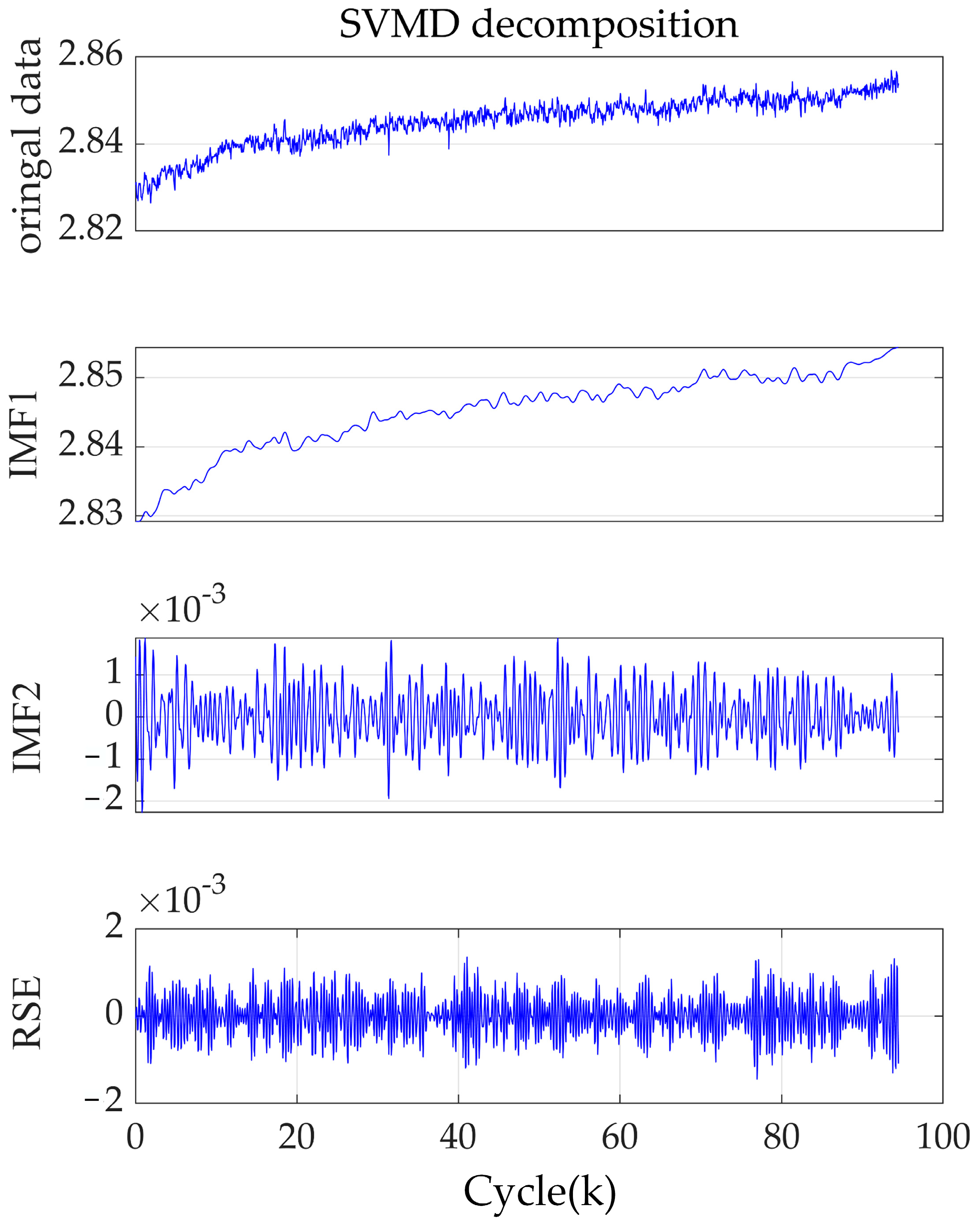
The obtained IMFs are sequentially designated as IMF₁, IMF₂, ..., IMF_L according to their center frequencies, arranged from low to high. Specifically, IMF₁ primarily reflects the trend of threshold voltage variations caused by degradation, whereas IMF₂ to IMF_L demonstrate the effects of load variations at different frequency levels on the threshold voltage. The residual signal error (RSE) is the remaining part after decomposition, induced by higher-frequency noise from the sampling circuit, and its influence can be neglected when the convergence tolerance is small. By applying SVMD, the original sequence is effectively decomposed into trend and fluctuation components.

2.2. Transformer Model

Transformer is a deep learning model that adopts a multi-head attention mechanism, which adaptively weighs the significance of each component of the input data. This mechanism allocates attention scores to various segments of the input, which influences the model’s focus during predictions. This approach captures long-range dependencies, thereby enhancing the model’s ability to recognize degradation of the SiC MOSFETs. Compared to RNN and LSTM, the Transformer leverages multi-head attention mechanisms to process data in parallel rather than sequentially [20,21,22]. The reduction in computational time contributes to its advantages. The Transformer’s self-attention mechanism can be described as follows.

(1) Calculate Query, Key, and Value Matrices: Query, Key, and Value matrices are used to calculate the attention scores, which are derived from the input. The detailed calculation process is shown in Equation (5).

$$Q=X\cdot W^Q,K=X\cdot W^K,V=X\cdot W^V$$

(5)

In the equation, Q, K, and V represent the results of encoding the input samples, followed by linear mapping. The matrix X denotes the input, while W^Q, W^K, and W^V are weight matrices.

(2) Calculate Attention Scores: Attention scores are calculated by performing a dot product between the Query and Key matrices. Following this operation, the resultant values are scaled, and the SoftMax function is applied to derive the final attention scores.

$$Attention(Q,K,V)=soft\max ({\displaystyle \frac{Q{K}^T}{\sqrt{d_K}}})V$$

(6)

In the equation, d_K is the dimensionality of the key vectors.

(3) Multi-Head Attention: The Transformer architecture employs multiple attention heads to capture various dimensions of the relationships present in the data. The results generated by these heads are combined and subjected to a linear transformation, as illustrated in Equation (7).

$$\begin{array}{l}MultiHead(Q,K,V)=Concat(hea{d}_i)W^O\\ where\begin{array}{cc}& hea{d}_i\end{array}=attention(Q{W}_i^Q,K{W}_i^K,V{W}_i^V)\end{array}$$

(7)

In the formula, head_i denotes the i-th attention, while W_i^Q, W_i^K, and W_i^V represent the different weight matrices associated with queries, keys, and values. The matrix W^O denotes the weight matrix for the output linear mapping, and k indicates the total number of attention heads. The parameters of the weight matrices can be learned through model training.

To effectively capture these temporal dependencies, this study employs a sliding window method for dataset reconstruction. This approach effectively addresses the challenge of limited data availability. In this study, the sliding window size is set to 20, with a step size of 1.

2.3. Sparrow Search Algorithm

The Sparrow Search Algorithm (SSA) is an optimization algorithm proposed based on the foraging behavior of sparrows during predation. This algorithm presents several advantages compared to EKF and PF, including robust optimization capabilities and rapid convergence speed [23,24,25]. In this study, a scenario involving n virtual sparrows that are engaged in the food search is considered, while the number of parameters that need to be optimized is d. The operation of this model is characterized by two distinct roles: discoverers and joiners.

Discoverers are sparrows with stronger foraging abilities, providing foraging directions for other sparrows. The position update of discoverers is shown in Equation (8).

$$X_{i,j}^{t+1}=\left\{\begin{array}{l}{X}_{i,j}^t\cdot \exp (-{\displaystyle \frac{i}{{\alpha }_{\mathrm{SSA}}\cdot ite{r}_{\max }}})\begin{array}{cc}& if:R_{SSA}<ST\end{array}\\ X_{i,j}^t+Q_{\mathrm{SSA}}\begin{array}{cc}& if:R_{\mathrm{SSA}}>ST\end{array}\end{array}\right.$$

(8)

In the formula, $X_{i,j}^t$ denotes the current position of the discoverers, iter_max denotes the total number of iterations, and α_SSA is a random number between 0 and 1. Q_SSA is a random number that obeys a normal distribution. R_SSA and ST denote the alarm value and the safety threshold, respectively. When R_SSA < ST, it indicates that there are no natural predators in the vicinity, and the explorer can conduct a global search. If R_SSA ≥ ST, it means that some sparrows have detected the presence of a predator, and all sparrows must take relevant actions.

Joiners should remain vigilant in monitoring the discoverers. Upon identifying superior food sources, they will promptly abandon the competition. The update of the joiners’ positions is represented in Equation (9).

$$X_{i,j}^{t+1}=\left\{\begin{array}{l}{Q}_{\mathrm{SSA}}\cdot \exp ({\displaystyle \frac{X_{worst}^t-X_{i,j}^t}{i^2}})\begin{array}{cc}& if\begin{array}{cc}& i>{\displaystyle \frac{n}{2}}\end{array}\end{array}\\ X_{best}^t-{\displaystyle \frac{1}{d}}\begin{array}{cc}{\displaystyle \sum _{j=1}^d\left|X_{i,j}^t-X_{best}^t\right|\cdot rand(\{-1,1\})}& otherwise\end{array}\end{array}\right.$$

(9)

In the formula, $X_{best}^t$ is the sparrow with the maximum fitness, and $X_{worst}^t$ is the sparrow with the minimum fitness.

When foraging, sparrows alter their foraging paths and emit alarm calls in response to the presence of predators. It is assumed that alarm-calling individuals constitute 10% of the total population, with their initial positions being randomly allocated. This behavior can be mathematically represented in Equation (10).

$$X_{i,j}^{t+1}=\left\{\begin{array}{l}{X}_{best}^t+\beta \cdot (X_{i,j}^t-X_{best}^t)\begin{array}{cc}& f_1\ne f_g\end{array}\\ X_{i,j}^t+K\left({\displaystyle \frac{X_{i,j}^t-X_{worst}^t}{\left|f_i-f_{worst}\right|+\epsilon }}\right)\begin{array}{cc}& f_1=f_g\end{array}\end{array}\right.$$

(10)

In the formula, β is a random number following a normal distribution with a mean of 0 and a variance of 1, and K is a random number within [−1, 1]. The parameter ε is a tiny number to prevent the denominator from being zero. f_worst is the worst fitness value, and f_g is the global optimal fitness value.

2.4. Overall RUL Prediction Framework Construction

The process of predicting the RUL of SiC MOSFETs involves several steps. Initially, raw V_th data is acquired through a power cycling circuit constructed with the device under test. This data is then subjected to outlier removal and linear interpolation for missing entries. The cleaned time-series data are then decomposed into a set of IMFs and RSE using the SVMD method.

During the training phase of the SSA-Transformer model, single-step prediction is employed. After dividing each IMF into training and test sets according to a predetermined ratio, training is conducted separately. By superimposing the prediction results of each IMF, the prediction value of V_th is obtained. RMSE and R² are selected as evaluation metrics to validate the model’s effectiveness.

The training process utilizes SSA to determine the optimal number of attention heads, learning rate, and regularization coefficient for the transformer model. A fitting function is established to minimize the RMSE, and the optimal solution is searched within defined upper and lower bounds. Under normal circumstances, the update step size decays exponentially, allowing it to approach the optimal solution gradually. Conversely, when a hazard is detected, the algorithm randomly generates an update step size to escape local optima. After the set number of iterations, the optimal hyperparameter values are returned. This optimization process is repeated 5 times, and the average of the three best solutions is taken to determine the final values of the model hyperparameters.

Finally, multi-step predictions are achieved through regression until the predicted value reaches the upper limit of V_th, at which point the step difference obtained is considered the RUL. To eliminate the impact of fluctuations on the prediction results, this design employs the sliding window method, where if the average of 5 consecutive predicted values exceeds the upper threshold, a failure is determined. Assuming the RUL prediction results follow a normal distribution, the prediction is repeated 10 times to obtain the variance and mean of the results, thereby determining the prediction interval with 95% confidence. The RUL prediction process is illustrated in Figure 1.

3. Experimental Setup and Execution

3.1. Aging Parameters Analysis

SiC power devices are subjected to multiple forms of stress, including electrical loading, thermal stresses, and mechanical vibrations. These factors contribute to the gradual degradation of the devices over time. As the degradation accumulates to a critical level, it may ultimately lead to the failure of the power devices. According to existing studies, the primary failure modes of SiC MOSFTs are gate oxide failures [26,27,28].

The primary cause of gate oxide failure in SiC MOSFETs is the generation and accumulation of defects within the gate oxide due to electro-thermal stress. During the turn-on and turn-off processes of power devices, carriers tunnel from the SiC semiconductor into the gate oxide under the influence of electrical and thermal stress. 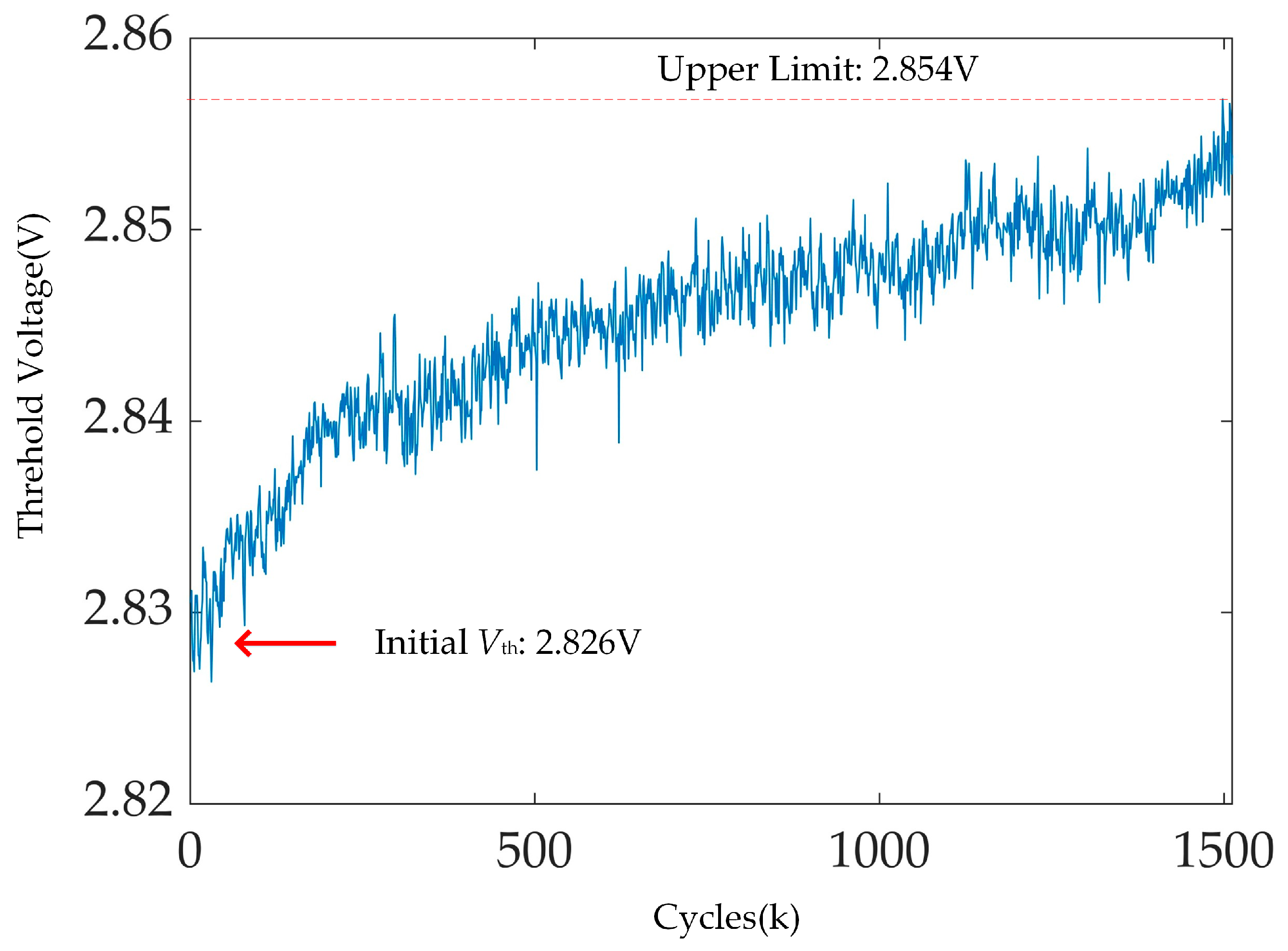These carriers become trapped by interface traps and oxide traps, resulting in a drift of V_th, a phenomenon known as bias temperature instability [29]. Therefore, the degree of gate oxide degradation can be intuitively assessed through changes in the threshold voltage. According to the AQG324 standard, the sample reaches its end-of-life state when V_th increases by 5%.

3.2. Experimental Setup

To obtain the degradation parameter V_th of SiC MOSFETs, a power cycling test platform is established. Power cycling test is a general method for evaluating the reliability of power devices. During the test, heat is generated inside the chip and dissipated through the packaging and cooling system, which is highly similar to actual operating conditions. 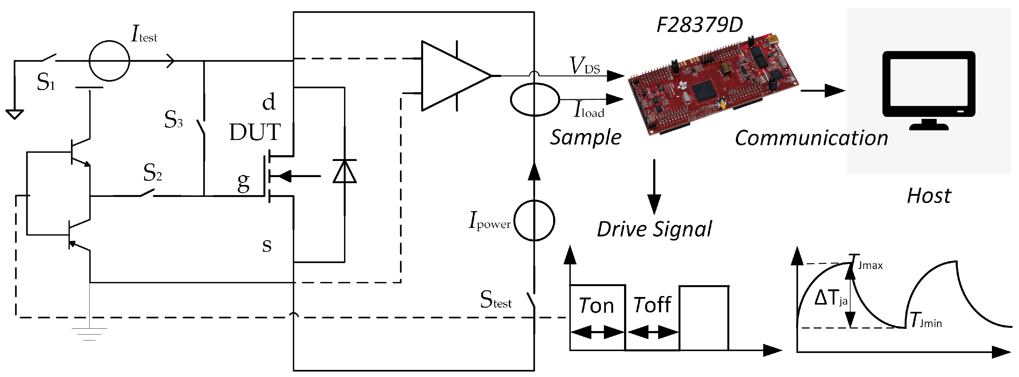Therefore, the power cycling test is considered the most realistic reliability assessment for power devices in practical applications [30,31,32]. The schematic diagram of the power cycling system is shown in Figure 2.

It mainly consists of three parts: the device under test, the driving section, and the sample section. The driving section is responsible for providing periodic current signals to the device under test. As illustrated in Figure 2, during the turn-on time, a current I_power is allowed to flow through the device under test, causing the chip junction temperature to rise. Conversely, during the turn-off time, no current flows through the MOSFETs, resulting in a decrease in the chip junction temperature. As the MOSFETs periodically switch on and off, the junction temperature of the chip fluctuates cyclically between the maximum value T_jmax and the minimum value T_jmin. These repeated temperature fluctuations can induce electro-thermo-mechanical stress in the gate oxide layer of the module. Over time, this stress can lead to the degradation of the module gate, ultimately resulting in device failure.

The sampling section is responsible for executing V_th sampling according to the specified cycle instructions. V_th is defined as the minimum gate-source voltage required for the device to turn on. When the drain-source current just reaches the preset value of on-state, the corresponding gate-source voltage V_gs is the threshold voltage of the MOSFET. Shorting the gate to the source is to utilize the constant current characteristic of the MOSFET saturation region, where the drain current I_d is solely determined by V_gs.

During power cycling, switches S₂ and S_test are closed, while switches S₁ and S₃ remain open. The activation and deactivation of the module are controlled by adjusting the drive signal to regulate the voltage across the gate-source V_GS. Upon reaching the designated number of cycles during power cycling, the sampling process is initiated: S₂ and S_test are opened, and S₁ and S₃ are closed. At this stage, the drive circuit and power supply are disconnected, and the gate and source of the device under test are shorted. The voltage between the drain and source, measured by the test current I_test, represents the V_th. In this study, I_test is set to 5 mA. To enhance measurement accuracy, three devices are evaluated using the designed circuit and a static power analyzer. The designed circuit is calibrated through linear fitting. The initial value of the V_th of the tested module is also obtained during this process.

3.3. Test Conditions & Data Acquisition

In this paper, the device under test selected is the NXH007P120M3F2PTHG, a SiC MOSFET module in F2 package from ONSEMI. This module has a rated current of 149 A, a maximum junction temperature of 175 °C, and an on-resistance of 7 mΩ.

A power test board is designed to provide the interface, driving signals, and an online sampling circuit for V_th to the SiC MOSFET. The control board used in this paper is the LAUNCHXL-F28379D, which is responsible for providing periodic driving signals, collecting, and uploading the sampled data.

In this study, the power cycling test achieved a junction temperature variation of 80 °C. The control signal is set to turn on for 5 s and turn off for 5 s. The load current is set to 150 A, and detection is completed using the Hall sensor DHAB S/125.

To enhance the junction temperature reduction rate of SiC MOSFETs during the turn-off phase, a water-cooling heat dissipation structure is incorporated into the test platform. The water-cooling radiator makes contact with the heat dissipation surface of the module through thermal grease, with the water flow rate set at 3.5 L/min. The chip junction temperature information is obtained by the NTC integrated inside the module. After the temperature field reaches equilibrium, the maximum junction temperature is 115 °C, and the minimum is 35 °C.

The sampling interval of the threshold voltage is set to 10 min, meaning sampling is performed every 60 power cycles. To ensure sampling consistency, the sampling moment is set at the end of the 60th cycle’s T_off period. After sampling is completed, the sampling circuit is disconnected and reconnected to the power cycling circuit. The switching action is performed by 4 MOSFETs, following the rule of opening first and then closing. The experimental conditions are listed in

Table 1. Experimental conditions of the power cycling test.

Parameter	Value
Iload	150 A
VGS	+18 V/−5 V
Ton	5 s
Toff	5 s
[Tjmin, Tjmax]	[35 °C, 115 °C]
Data collection	every 10 min
Ambient temperature	30 ± 2 °C
Cooling water flow rate	3.5 L/min

.

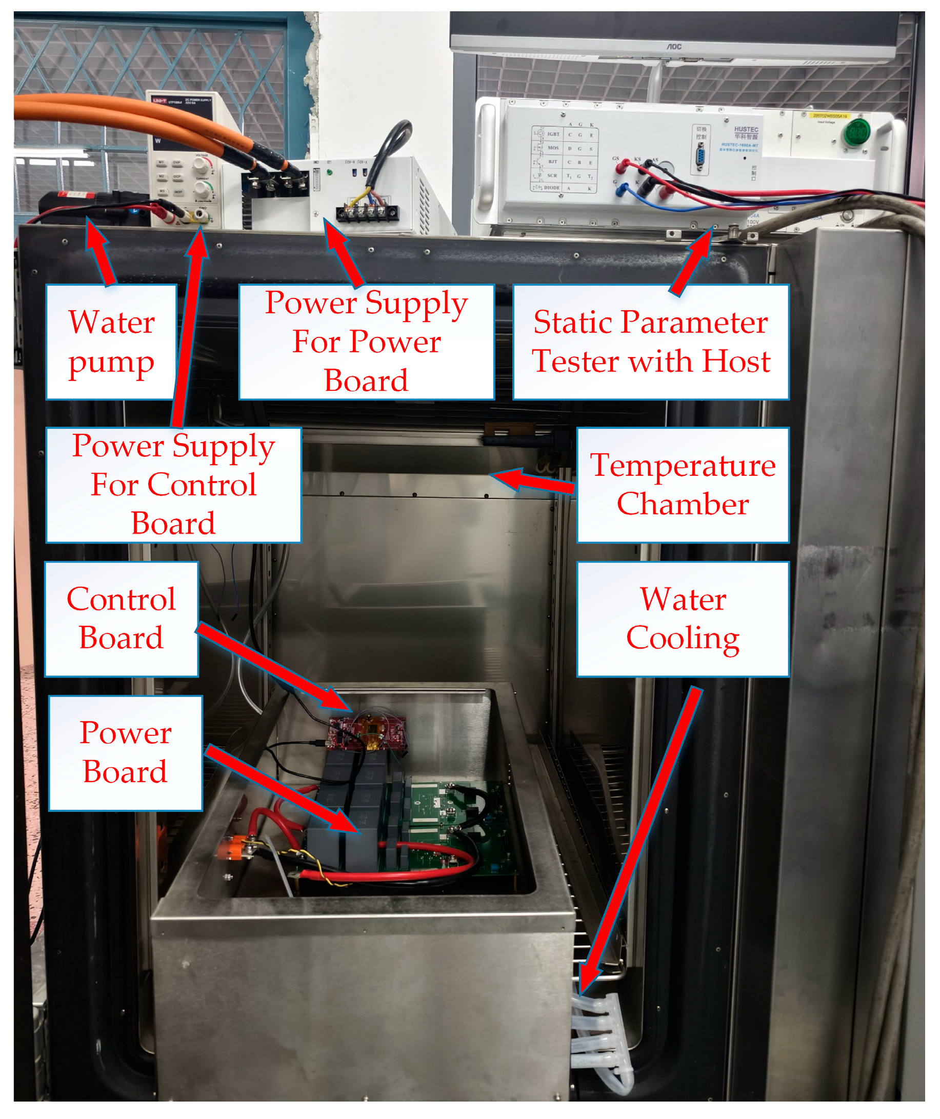
The power cycling test is performed in a temperature chamber to prevent the influence of ambient temperature changes on the aging process. The temperature fluctuation is within 0.5 °C Celsius, and the temperature deviation is within 2 °C Celsius. The test bench is shown in Figure 3.

4. Results

4.1. Model Parameter Settings

On the power cycling test platform designed in this research, 1512 data points were collected over 252 h. The obtained data are shown in Figure 4. After outlier removal and linear interpolation, these data constitute the dataset for this predictive model. It should be noted that this study selects 1% as the threshold for bias voltage degradation upper limit, instead of the commonly used 5%. Under the same sampling time interval, a larger bias voltage range generates a larger volume of data and also increases the number of steps for regression prediction. Of course, such issues can be effectively resolved by increasing the sampling time interval, but the time cost for the threshold degradation test will be significantly increased. This study primarily focuses on the trend changes of devices under aging stress, rather than the performance of devices reaching a specific level of damage. Therefore, to reduce time costs, the upper threshold is determined to be 1%.

The parameters of the dataset are shown in

Table 2. Parameters of the V_th dataset.

Parameters	Value
Dataset scale	1512
Proportion of test set	20%
Initial threshold voltage	2.826 V
Threshold voltage upper limit	2.854 V
Cycle to failure	1496

.

As a key parameter in SVMD, penalty factor α_SVMD is used to balance the data fidelity constraint and the mode compactness. A smaller α_SVMD emphasizes signal fidelity but results in less concentrated spectra. Conversely, a larger α_SVMD prioritizes signal compactness, leading to more concentrated spectra, but with greater reconstruction errors. Considering the lenient requirement for model compactness in this study, α_SVMD is set to 1000. The parameter configuration of SVMD is shown in

Table 3. Parameter settings of SVMD.

Parameters	Value
Penalty factor (αSVMD)	1000
Time-step of the dual ascent (tau)	0
Tolerance of convergence criterion (tol)	1 × 10−6

.

The decomposition results of the degradation data by SVMD are shown in Figure 5. V_th can be observed to have been decomposed into 3 components containing different features. IMF₁ represents the long-term trend of threshold voltage degradation, IMF₂ represents the response to load fluctuations, and RSE is the residual. Since the load is constant in this experiment, the fluctuation component only includes IMF₂ with a small weight.

After decomposing into various IMFs through SVMD, each is input into the corresponding SSA-Transformer for training. SSA is used to obtain the optimal combination of Transformer hyperparameters corresponding to the input data. The key parameters of SSA are shown in

Table 4. Parameter settings of SSA.

Parameters	Value
Pop_size	30
Max_iter	20
Discover_rate	20%
Alarmer_rate	10%

. The hyperparameters optimized using SSA include the number of attention heads, initial learning rate, and regularization coefficient. Their search ranges and final optimization results are shown in

Table 5. The upper and lower boundaries and the optimal values of the Transformer model.

Parameters	Scope	Optimal Value
Self-attention mechanism heads	[2, 64]	24
Learning rate	[1 × 10−6, 1 × 10−1]	1.7 × 10−3
Dropout rate	[1 × 10−5, 1 × 10−1]	8.7 × 10−2

.

When using a transformer for time series prediction, some other parameter configurations are shown in

Table 6. Some other parameter settings of the Transformer model.

Parameters	Title 2
D_model	32
Optimizer	Adam
MaxEpochs	100
MiniBatchSize	256

.

4.2. Evaluation Metrics

The comparative predictive efficacy of the suggested algorithms against other deep learning techniques can be quantitatively assessed through the use of the coefficient of determination R² and the RMSE. RMSE evaluates the prediction performance from the dimensions of error magnitude and accuracy, where smaller values indicate higher prediction accuracy of the model. R² measures the model’s fitting effect on the data, with larger R² values indicating a better fit. The calculation of these parameters is shown in Equations (11) and (12).

$$RMSE=\sqrt{{\displaystyle \frac{1}{n}}{\displaystyle \sum _{i=1}^n{e_i}^2}}=\sqrt{{\displaystyle \frac{1}{n}}{\displaystyle \sum _{i=1}^n{(y_i-\stackrel{\wedge }{y_i})}^2}}$$

(11)

$$R^2=1-{\displaystyle \frac{{\displaystyle \sum _{i=1}^n{(y_i-\stackrel{\wedge }{y_i})}^2}}{{\displaystyle \sum _{i=1}^n{(y_i-\overline{y_i})}^2}}}$$

(12)

4.3. Result Analysis

To demonstrate that the introduction of SVMD and SSA significantly enhances the performance of Transformer-based aging prediction, a comparative experiment is conducted using two algorithms: Transformer and SVMD-Transformer.

Figure 6 presents the prediction results obtained by applying a single Transformer model. The original signal of the threshold voltage contains high-frequency fluctuations, and the model faces a trade-off between overfitting and simulation accuracy, resulting in suboptimal prediction performance.

Figure 7 demonstrates the effect of first decomposing the original signal and then applying the transformer for prediction. After the threshold voltage is decomposed by SVMD, the trend component and fluctuations are retained, while the high-frequency residuals are discarded. This approach ensures prediction accuracy while avoiding overfitting.

Figure 8 illustrates the predictive performance of the model proposed in this study. The original signal is first decomposed, and then the transformer is applied for prediction. SSA is utilized for hyperparameter optimization of the transformer to achieve better predictive performance. As shown in the figure, the optimized hyperparameters result in a closer match to the actual trend and a more detailed reproduction of fluctuations.

To quantitatively evaluate the three models, the test set is used to calculate the R² and RMSE. Figure 9 shows the box plots of R² and RMSE obtained from 10 repeated experiments, displaying the mean and fluctuation range of the evaluation metrics. By integrating SVMD, the model achieved two key improvements: it effectively lowered the RMSE and elevated the R². Meanwhile, SSA-based optimization not only enhanced the stability of the model output but also brought a certain degree of improvement to its predictive performance. The R² value exceeds that of both the Transformer and SVMD-Transformer by 78.5% and 10.2%, respectively. Furthermore, the RMSE is lower than that of the transformer and SVMD-Transformer by 85.9% and 46.8%, respectively. These findings clearly demonstrate that the application of SVMD and SSA significantly improves both the prediction accuracy and robustness of the Transformer model.

Applying the optimal hyperparameters of the Transformer, recursive prediction is conducted starting from the 1210th data point, with the interval to reach the threshold voltage upper limit recorded as the RUL reference value. The experiment is repeated 10 times, yielding a mean of 289.5 and a standard deviation of 6.7 from the experimental data. Assuming the prediction results follow a normal distribution, the 95% confidence interval is obtained as [285, 294] according to Equation (13), while the actual value was 286. This validates the effectiveness of the prediction.

$$95\%confidence interval:[\overline{X}-1.96{\displaystyle \frac{s}{\sqrt{n}}},\overline{X}+1.96{\displaystyle \frac{s}{\sqrt{n}}}]$$

(13)

5. Conclusions

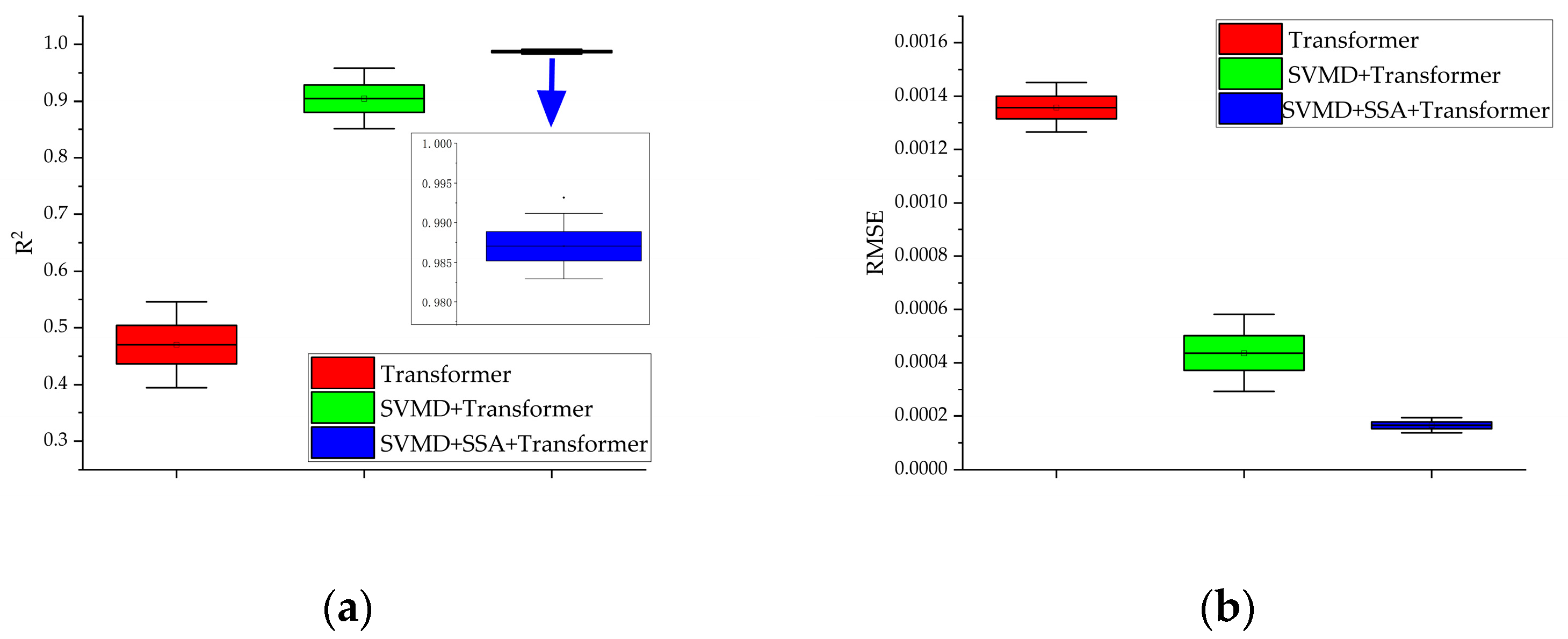
This study proposes an integrated SVMD-SSA-Transformer model to address challenges in SiC MOSFET RUL prediction. The proposed framework encompasses degradation feature selection, data preprocessing, model optimization, and multi-component prediction, providing a scientific solution for power device RUL assessment. Specifically, V_th is selected as the core degradation feature, with real data collected via a power cycling platform; SVMD decomposed chaotic V_th signals into trend and fluctuation components, separating degradation features from load interference and enhancing feature extraction efficiency; and the SSA adaptively optimized Transformer hyperparameters, reducing manual configuration blindness, solving the poor generalization of fixed hyperparameters, and balancing accuracy and robustness. Comparative experiments confirm the model’s superiority, including significantly higher R² and lower RMSE than traditional models and enhanced output stability via SSA optimization. In terms of application and significance, the model is directly applicable to SiC MOSFET RUL assessment, which provides accurate device replacement timelines to avoid system failures and improve application reliability.

This study has the following limitations in experimental design and data acquisition. First, the relatively small sample size and limited variety of samples may restrict the statistical representativeness and generalizability of the research findings. The applicability of this model will be further validated in future studies. Second, the experiment relies solely on a single stress profile, failing to encompass the stress conditions present in various real-world application scenarios, which makes it difficult to comprehensively reflect the aging patterns of equipment under complex working conditions. In the future, we will use finite element simulation software to study the impact of multiple stresses on degradation.