Comparative Analysis of Traditional Statistical Models and Deep Learning Architectures for Photovoltaic Energy Forecasting Using Meteorological Data

Abstract

The integration of photovoltaic (PV) energy into the power grid requires precise forecasting due to its dependence on the variability of weather conditions. This study explores the effectiveness of neural network models for predicting PV energy generation using historical meteorological and temporal data from Austria over a two-year period. We implement and compare multiple neural machine learning approaches, including Multilayer Perceptrons (MLPs), Recurrent Neural Networks (RNNs), and Convolutional Neural Networks (CNNs), against traditional statistical models such as Decision Trees (DTs), Linear Regression (LR), and Random Forest (RF). Our methodology introduces novel data preprocessing techniques, including cyclical encoding of time features, to improve prediction accuracy. Results demonstrate that RNN models outperform other architectures in single-step forecasting, achieving a Mean Squared Error (MSE) of 0.045 and a Mean Absolute Error (MAE) of 0.0427, while CNNs prove superior for multi-step predictions. These findings highlight the potential benefits of applying predictive deep learning techniques for optimal PV energy management, contributing to grid stability and sustainability. This study systematically compares the effectiveness of traditional and deep learning models for photovoltaic energy prediction under the same data preprocessing conditions, including the cyclical encoding of temporal features that provides a continuous representation of the time frame allowing its use as an input feature. This study identifies the specific strengths of each model (RNN for single-step prediction, CNN for multi-step prediction) for Central European climates, validated on Austria’s unique meteorological dataset.

1. Introduction

In recent decades, the addition of renewable energy installations to the power grid has caused an exponential growth in the global electricity distribution system. This growth can be attributed to a number of factors, such as a significant increase in consumption, increased awareness of the environmental damage caused by the production of energy from fossil fuels, and the foreseeable limited availability of fossil fuels [1,2,3].

Photovoltaic (PV) electricity generation, also referred to as solar power, is the product of the conversion of solar radiation through a semiconductor device called a photovoltaic cell [4]. Solar radiation is a renewable, inexhaustible, and non-polluting energy source. The benefits of this technology include the following: (a) there are no greenhouse gas emissions, (b) the possibility of safely storing energy in batteries, (c) ease of implementation and installation at both industrial and residential levels, and (d) its production also leaves a smaller carbon footprint on the environment compared to other energy sources [5].

The amount of PV energy generation is uncertain, mostly due to meteorological variability and panel physical degradation, introducing stability issues in the electricity distribution grid when PV modules are plugged in. Consequently, there has been an increased need to protect the grid, using techniques such as the implementation of distributed generation plants reducing the dependence on large transmission networks, and  the prediction of the amount of PV energy generation [6] using Machine Learning (ML) and other Artificial Intelligence (AI) tools [7,8] exploiting various data sources, including weather data [9]. An accurate prediction will allow better planning of the mix of the generation of electric energy throughout the day since different electricity generation technologies have different orders of response time to commands to increase or decrease production, ranging from weeks for nuclear reactors, several minutes for fossil fuel thermal plants, down to seconds for hydroelectric reservoir systems.

The difficulty of acquiring high-quality data in real time is a major obstacle for the training of robust models capable of taking into account dynamic environmental conditions and making precise adjustments. Addressing these challenges can improve PV energy management and its safe embedding in the global electric grid. In addition, to maintain its stability, the electric grid must be in continuous balance between generation and demand, which becomes increasingly complex as tensions are reduced and demands are disaggregated.

The advent of the PV energy generation technology has given rise to the so-called prosumers, consumers who have private PV installations connected to the grid selling surplus energy to the grid. Hence, further complicating the situation are the highly variable and non-linear characteristics of energy use in buildings, which depend largely on individual consumer habits. Availability of a power generation predictive tools can benefit prosumers by allowing them to make informed decisions about their energy use, adapting their consumption to their generation patterns, based on forecasts. Through better planning energy consumption and production, their dependence on centralized electricity grids can be reduced, encouraging energy self-sufficiency and sustainability, while improving energy security by minimizing uncertainty in supply.

For big energy operators, accurate predictions allow better anticipation of fluctuations in solar energy generation and to make informed decisions in order to ensure a stable supply of energy during periods of peak demand. This ensures a stable energy supply for the community, minimizing the risk of power outages or shortages.

Predictive tools could also enable off-grid communities depending on local PV systems to predict energy availability, enabling better planning of daily activities, thus improving the overall quality of life in remote regions.

In summary, the benefits mentioned will have a positive economic impact on the people and communities that make use of PV energy generation. Facilitating the integration of solar energy into the grid, greenhouse gas emissions can be reduced. In this way, the global dependence on fossil fuels to generate electricity is reduced, which translates into a cleaner environment while contributing to the fight against climate change.

This paper contributes a resourceful use of cyclical time transformations to enable the use of the time axis as an additional variable of the models and the analysis of different models under specific conditions ranging from the baseline model Linear Regression (LR) up to more advanced DL approaches. While LR is widely used in many studies, its linear nature limits its capacity to capture complex patterns in PV energy generation.

The key novelties of this work are as follows: (i) a comparative evaluation of classical and neural network-based models for PV energy prediction exploiting weather and power generation historical data, (ii) the use of cyclical transformations of temporal labels in order to introduce them in the models, thus enhancing model performance, (iii) the recommendation of model types based on forecast horizons, and (iv) a reproducible computational pipeline using public datasets and open-source tools.

The rest of this paper is structured as follows: Section 2 reviews the state of the art. Section 3 describes materials and methods. Section 4 shows experimental results. Section 5 concludes this paper.

2. State of the Art

A summary of the most salient features of the relevant references found in the state-of-the-art examination are given in Table 1. Combined with material and technological innovation in power electronics [10,11], Artificial Intelligence’s (AI) contribution would translate into cost reduction, making PV energy generation more competitive and allowing it to penetrate further into the global energy market, displacing traditional energy sources such as fossil fuels. It may also play a role in the realization of a circular market for renewable energy technologies, allowing more efficient recycling [12], and in the creation of smart grids for smart city development [13].

Machine Learning (ML) and AI techniques have been extensively recognized as useful tools for the improvement of the efficiency and safety of renewable energies, solar, wind and marine [14,15,16], including the aggregation of several renewable energy sources [17]. A recent overview [18] of AI applications in PV systems focuses on three main areas: Maximum Power Point Tracking (MPPT) monitoring, power generation prediction, and fault detection. It analyzes the potential impact of AI in this area, considering its use to increase efficiency, safety, and forecasting performance.

Regarding MPPT, AI can help to optimize the performance of PV energy generation by continuously adjusting their orientation relative to the sun to capture the maximum amount of energy possible. For instance, the relation between the temperature at the PV module surface and the generated power can be modeled by AI techniques [19]. On the other hand, in AI application to power generation prediction, historical power generation and weather data can be analyzed to estimate real-time and future solar energy production. Finally, in the area of fault detection, AI can identify problems or breakdown risk based on early symptoms in order to take appropriate corrective measures in time [20]. Other reviews [21] deal with the use of ML for the planning of energy production for the control of the energy market.

A more specific review of Deep Learning (DL) techniques for predicting PV power generation [22] highlights the Long-Short Term Memory (LSTM) technique for its effectiveness compared to other types of architecture for all time horizons and how Gated Recurrent Unit (GRU) might work better when there is a reduced amount of data to work with. This work also proposes a new DL model architecture to predict industrial PV generation that tackles a universe of problems that can be found in this context, proposing their respective solutions with the aim of maximizing the effectiveness of its prediction. This model considers as input the results of solar radiation and temperature prediction models, the solar PV installation, its degradation, the operation and maintenance data of the plant, radiation, temperature, and efficiency historical data of the installation.Other works [23] apply a dung beetle optimization approach to the hyperparameter tuning of bidirectional LSTMs for ultra-short-term PV energy generation forecasting.

Since forecasting power generation from renewable sources is a current hot topic, application of AI is addressed from many different points of view. For instance, Artificial Neural Networks (ANNs) [24,25,26,27] and other regression models such as K-Nearest Neighbors [28,29], Fuzzy C-means [30], hierarchical non-linear autorregressive exogenous regression [31], quantile regression [32], and hybrid regression mixing Random Forests and LSTMs [33] are proposed for these forecasting tasks, while other works [34] compare several regression approaches, such as Support Vector regression (SVR) and Gaussian Process regression (GPR), over specific datasets. Multi-objective PSO (MOPSO) for training Artificial Neural Networks (ANNs) has been proposed for solar energy generation forecasting [35], while other approaches focus on the use of recurrent neural networks for the same task [36]. Regarding other sources of renewable energy, prediction of wind speed has been proposed using Regression GRUs [37] while Long-Short term memory LSTM [38] and transformer encoders have been demonstrated for prediction of marine energy generation [39].

A model for predicting PV energy generation based on meteorological, temporal, and geographic data from 12 installations in the United States is proposed in [40]. This model excludes irradiance modeling, despite the fact that it is usually considered as very relevant in this type of study [41,42,43,44], due to the practical difficulty of obtaining reliable values. Various validation and evaluation methods were analyzed for 4 different approaches based on the distribution of the training and test data, and whether the data corresponded to the 12 locations or the model was for a specific location. The best results were obtained using Random Forest (RF). Only in 4 of the 12 locations it was better to use exclusively the data from one location. The importance of customizing the prediction models for each specific location to optimize the performance of the models is concluded by the authors. Other works [45] use multiple weather features in order to improve the performance of PV energy generation prediction in zero energy consumption buildings or for the day-ahead prediction of the on-site PV energy generation [46] by data augmentation of local Internet of Things data. Multi-model dynamic combinations using credible weather models are also proposed for short-term PV power generation forecast [47], while clustering the weather features seems to provide advantages in a double layer prediction model that uses GRU-informer and SVRs [48]. Similar approaches search for similar weather days by a sparrow optimization algorithm [49].

Another work [50] compares 24 different machine learning models for the prediction of power output for the next day for 16 PV plants located in Hungary, testing the models over a 2-year period, with at a 15 min resolution for 16 PV plants. The study focused on ready-to-use ML models from a high-level software library (using 21 algorithms from the scikit-learn library and 3 from independent packages (XGBoost, LGBM, CatBoost)). Before training the models, data pre-processing was performed, including removal of night-time data and data from time points with zero power generation, as well as the normalization of inputs and outputs. In addition to analyzing the performance of these models, they also test the effect of the prediction selector and the tuning of hyperparameters. Reviewing their results, the authors concluded that the most accurate model is the Ridge Kernel regression; however, it has the disadvantage of being very slow and using a lot of memory. On the other hand, they highlight how the Multilayer Perceptron (MLP) has a similar accuracy but a shorter training time. Therefore, the authors recommend the first one for scientific research and the second one for practical cases.

The choice of input data may be more relevant than the choice of model [50]: comparing the results using the basic input meteorological data with one that complements it with sun position angles and processed irradiance values, a reduction in the Root Mean Square Error (RMSE) value of 13.1% is achieved. Likewise, the adjustment of the hyperparameters is highlighted as a vital procedure to exploit the potential of the models to the maximum. In the case study [50], they achieved a reduction of 3.1% of the $RMSE$ when compared to the model with the default parameter values. While in the most robust models the difference between using the default hyperparameters or the adjusted ones barely makes a difference, for other models it is vital to avoid errors.

Prediction of energy production in a building-integrated PV system using ML algorithms based on data obtained from a residential photovoltaic installation was reported in [51]. The models use both supervisory Control and Data Acquisition (SCADA) data of electrical production and meteorological data from a measurement installation. The authors analyse 5 ML models (namely RF, Decision Trees, XGBoost, LightGBM, and CatBoost) in conjunction with hyperparameter optimization using grid search to predict hourly power generation from PV, concluding that LightGBM is the most suitable in this context, with results of 0.96 $R^2$. It is also concluded that solar radiation, air temperature, relative humidity, and time of day were the most important features for the model. Table 1 summarizes the revised literature.

Table 1. Comparison of the best-performing models with the State of the Art.

Study (Year)	Model(s) Used	Dataset	Prediction Type	Key Results
Aravena-Cifuentes et al. (2025)	RNN (LSTM), CNN, MLP, DT, LR, RF	Austria (2015–2017)	Single-step: 1 h Multi-step: 24 h	Single-step: RNN (MSE = 0.0045, MAE = 0.0427) Multi-step: CNN (MSE = 0.1956, MAE = 0.2367)
Zoubir et al. (2024) [51]	LightGBM, RF, XGBoost, CatBoost, DT	Residential PV (Morocco)	Hourly	LightGBM (MAE = 0.180, $R^2$ = 0.96)
Quan et al. (2024) [23]	Dung beetle-optimized BiLSTM	Industrial PV	Ultra-short-term	Optimized BiLSTM outperformed standard LSTMs/GRUs (MAE = 0.175)
Chandel et al. (2023) [22]	LSTM, GRU, hybrid DL	Industrial PV	Multi-horizon	LSTM best for all horizons; GRU better with limited data
	Hybrid: Wavelet, DCNN, Quantile Regression		15, 30, 60, and 120 min	MAPE: 0.0382–0.0385 RMSE: 3.8772–14.3381 MAE: 2.0340–8.0759
	Hybrid: CNN, Variational Mode Decomposition		60, 360, and 720 min	RMSE-2.0533 MAE-1.5418 MASE-0.1752
	Hybrid: GRU K-means clustering		12 step size	MAE: 0.0379–0.0409 RMSE: 0.0683–0.725
	PM, ARIMAX, MLP, LSTM, ALSTM		7.5, 15, 30, and 60 min	60 min MAE: PM 2.12 ARIMAX 1.98 MLP 1.63 LSTM 1.48 ALSTM 1.47
Li et al. (2023) [45]	FCM ISD MAOA ESN	Zero-energy buildings	Short-term	MAE: 0.16639
Park et al. (2022) [46]	POST-enCNN	On-site PV (Korea)	Day-ahead	MAE: 2.15 RMSE: 3.83 MAPE(%): 51.7

Table 1. Comparison of the best-performing models with the State of the Art.

Study (Year)	Model(s) Used	Dataset	Prediction Type	Key Results
Aravena-Cifuentes et al. (2025)	RNN (LSTM), CNN, MLP, DT, LR, RF	Austria (2015–2017)	Single-step: 1 h Multi-step: 24 h	Single-step: RNN (MSE = 0.0045, MAE = 0.0427) Multi-step: CNN (MSE = 0.1956, MAE = 0.2367)
Zoubir et al. (2024) [51]	LightGBM, RF, XGBoost, CatBoost, DT	Residential PV (Morocco)	Hourly	LightGBM (MAE = 0.180, $R^2$ = 0.96)
Quan et al. (2024) [23]	Dung beetle-optimized BiLSTM	Industrial PV	Ultra-short-term	Optimized BiLSTM outperformed standard LSTMs/GRUs (MAE = 0.175)
Chandel et al. (2023) [22]	LSTM, GRU, hybrid DL	Industrial PV	Multi-horizon	LSTM best for all horizons; GRU better with limited data
	Hybrid: Wavelet, DCNN, Quantile Regression		15, 30, 60, and 120 min	MAPE: 0.0382–0.0385 RMSE: 3.8772–14.3381 MAE: 2.0340–8.0759
	Hybrid: CNN, Variational Mode Decomposition		60, 360, and 720 min	RMSE-2.0533 MAE-1.5418 MASE-0.1752
	Hybrid: GRU K-means clustering		12 step size	MAE: 0.0379–0.0409 RMSE: 0.0683–0.725
	PM, ARIMAX, MLP, LSTM, ALSTM		7.5, 15, 30, and 60 min	60 min MAE: PM 2.12 ARIMAX 1.98 MLP 1.63 LSTM 1.48 ALSTM 1.47
Li et al. (2023) [45]	FCM ISD MAOA ESN	Zero-energy buildings	Short-term	MAE: 0.16639
Park et al. (2022) [46]	POST-enCNN	On-site PV (Korea)	Day-ahead	MAE: 2.15 RMSE: 3.83 MAPE(%): 51.7

3. Materials and Methods

3.1. Software and Hardware

Experiments are carried out on a laptop with Intel Core i5-10300H CPU clocked at 2.5 GHz. The machine is equipped with 8 GB DDR4 RAM and uses 16.8 GB of virtual memory. Python 3.11.9 language is used to implement the computational experiments. We use the following libraries: tensorflow, tensorflow.keras, keras tuner, visualkeras, and Scikit-learn.

The hyperparameter optimization algorithm is a structured code for training a deep learning model using TensorFlow and Keras Tuner. First, global parameters such as the maximum number of epochs and the directory for storing trained models are defined. The buildModel(hp) function constructs a sequential neural network with Conv1D and LSTM layers, where filters, kernel size, and activation function are selected through hyperparameter tuning. Then, the compileAndFit(model, name, window, patience) function trains the model using Early Stopping to prevent overfitting and ModelCheckpoint to save the best model. After that, a Tuner is configured to explore hyperparameter combinations through a random search with up to 50 trials. Finally, the best model is selected, its summary is displayed, its structure is visualized, and it is trained using the best hyperparameters found.

3.2. Dataset

This work uses two open access datasets downloaded from the Open Power System Data site (https://open-power-system-data.org/background/, (accessed on 24 April 2024)) [52] that are relevant for energy modeling in Europe: Time Series Data [53] and Weather Data [54].

The imported datasets include historical generation and consumption time series data (‘time series 60 min singleindex filter’) and weather data (‘weather data filtered.csv’) are provided in Supplementary Materials. These datasets were merged based on the ‘utc timestamp’ column using an inner join, ensuring that only records with matching timestamps were included.

3.2.1. Time Series Data

This dataset cover 37 European countries. It is available in resolutions of 15, 30, and 60 min. Depending on the country and the chosen time resolution, it can include data on electricity consumption (load), wind and solar power generation, installed capacity, and electricity prices. For hourly resolution, the dataset is contained in a single CSV file of 108,818 rows and 217 columns. The computational experiments reported below are carried out over the data from Austria. The variables included are briefly described below:

• Generation and Consumption

  –

  X_solar_generation_actual: (number): PV energy generation in the country X in MW.

  –

  X_wind_onshore_generation_actual: (number): onshore wind energy generation in country X in MW.

  –

  X_load_entsoe_transparency: (number): total load in country X in MW obtained from ENTSO-E Transparency Platform.

  –

  X_load_entsoe_power_statistics: (number): total load in country X in MW obtained from ENTSO-E Data Portal/Power Statistics.

• Temporal

  –

  utc_timestamp: (datetime): date and time of measurement in UTC format.

  –

  cet_cest_timestamp: (datetime): date and time of measurement in CET-CEST format.

• Other

  –

  interpolated_values: (text): columns where missing values in the original database were estimated by interpolation.

  –

  X_price_day_ahead: (number): daily spot price for country X in Euro per MW/h.

3.2.2. Weather Data

This dataset contains aggregated weather data in hourly resolution for 10 countries in Europe, including data for different NUTS-2 zones in Germany. Hourly aggregated weather data is generated from a weighted average of the data from each country. The dataset has been compiled by downloading, resampling, and merging data from several sources into a single CSV file of 324,361 rows and 193 columns. Depending on the country, the time range of the obtained data can range from 1980 to 2016. The computational experiments reported below are carried out over the data from Austria.

• Meteorological

  –

  X_windspeed_10m (float number): wind speed at 10 m height in country X in ${\displaystyle \frac{\mathrm{m}}{\mathrm{s}}}$.

  –

  X_temperature (float number): temperature in country X in °C.

  –

  X_radiation_direct_horizontal (float number): horizontal direct radiation for country X in ${\displaystyle \frac{\mathrm{W}}{{\mathrm{m}}^2}}$.

  –

  X_radiation_diffuse_horizontal (float number): horizontal diffuse radiation for country X in ${\displaystyle \frac{\mathrm{W}}{{\mathrm{m}}^2}}$.

• Temporal

  –

  utc_timestamp (datetime): date and time of measurement in UTC format.

We renamed relevant columns to improve readability, removing variables that were not used in the modeling process. The ‘utc timestamp’ column was also converted into a datetime format to facilitate time-based feature engineering.

3.3. Preprocessing—Austria Case Study

In this paper, we use only the data corresponding to Austria (called AT in the original database) in hourly resolution and already filtered as provided directly by the website. The Austria dataset combines the country data from the two databases mentioned in the previous section: Time Series Data and Weather Data.

• Time Series Data: This dataset has 108,818 rows and 7 columns, which have information on electricity consumption and solar and wind power generation covering from 31 December 2005 up to 31 May 2018. It is important to note that daily spot price data is not available in this dataset.
• Weather Data: This dataset has 324,361 rows and 5 columns and contains all the weather variables mentioned above. It covers the period from 1 January 1980 to 30 June 2017.

The time series and weather data were fused using the reference of the utc_timestamp key, allowing both sources of information to be combined into a single DataFrame. This column was converted to a suitable date and time format (i.e., datetime).

Since this work seeks to make predictions one hour into the future, it was verified that the data sampling rate was one hour uniformly for all variables and the duration of the studied time span. Data from earlier years is not representative of the actual state of the electric grid, because the number of PV and wind energy installations have grown exponentially in recent years. Therefore, the analysis in this paper uses only the data corresponding to the most recent years available in both datasets, namely the years 2015, 2016, and 2017. Furthermore, in these years, the variables collected in this dataset have no missing values (NaN), so no data imputations are necessary. After this time selection, the consolidated database contains 21,888 rows and 8 columns.

Finally, we give below the variable renaming conducted to facilitate readability of the results:

• utc_timestamp → date_time
• AT_solar_generation_current → portal_load
• AT_wind_onshore_generation_current → calculated_load
• AT_load_entsoe_transparency → solar_generation
• AT_load_entsoe_power_statistics → wind_generation
• AT_temperature → temperature
• AT_radiation_direct_horizontal → radiation_direct
• AT_radiation_diffuse_horizontal → radiation_diffuse

3.4. Feature Engineering

3.4.1. Circular Time Features

As the target application seeks to predict future events by considering past data with strong temporal components, the date and time of the day when the measurements are taken are useful for induction of temporal patterns such as trend or seasonality improving the accuracy of the model.

However, in order to fully exploit the information of these time variables, they must be represented appropriately, since it is impossible for any predictive model to ’discover’ the circular value space of the hours of the day, the days of the week, and the months of the year, e.g., the fact that the hour 24 of one day is the same as the hour 0 of the next day cannot be extracted numerically from the conventional date and time representation. Moreover, night and daylight have a strong influence on both demand and PV energy generation. For these reasons, it is imperative to encode them in a way that represents faithfully this cyclical nature [55].

For the models evaluated in this paper, the format of the variable “date_time” is not adequate to be used as input to any predictive model, hence we transform it into a continuous smooth variable as follows. First, it was converted from datetime format into seconds. We first define the period of one day as $24\times 60\times 60$ = 86,400 s. The period of a year is approximated as $365.2425\times 24\times 60\times 60=\mathrm{31,557,600}$ s. However, this transformation is not enough, we need to consider the time data periodicity using the sine and cosine transformations, which preserve the cyclic characteristics of the variable as coordinates on a circle [55,56]. This transformation encodes the time of day as a point on a unit circle, ensuring that times near midnight are close to those near the start of the day, and ensuring that the seconds at the end of December 31st are close to the seconds at the beginning of January 1st. This transformation is essential, since incorrect handling of time variables can significantly affect the results and the convergence of the algorithms [57]. After this variable transformation, we performed feature selection by removing variables that were not directly relevant to the prediction task, such as “portal load”, “calculated load”, “wind generation”, and “windspeed 10 m”.

To assess the impact of this transformation, we compare the predictive performance of models with and without the cyclic time transformation. The results show that models incorporating these cyclic transformations yield improved accuracy, exploiting the periodic nature of the data. This improvement is particularly evident in scenarios where time-related patterns—such as daily peaks or seasonal variations—are important for prediction.

3.4.2. Correlation Analysis

The Pearson correlation coefficient, defined by Equation (1)

$$r_{xy}={\displaystyle \frac{{\sum }_{i=1}^n(x_i-\overline{x})(y_i-\overline{y})}{\sqrt{{\sum }_{i=1}^n{(x_i-\overline{x})}^2}\sqrt{{\sum }_{i=1}^n{(y_i-\overline{y})}^2}}}$$

(1)

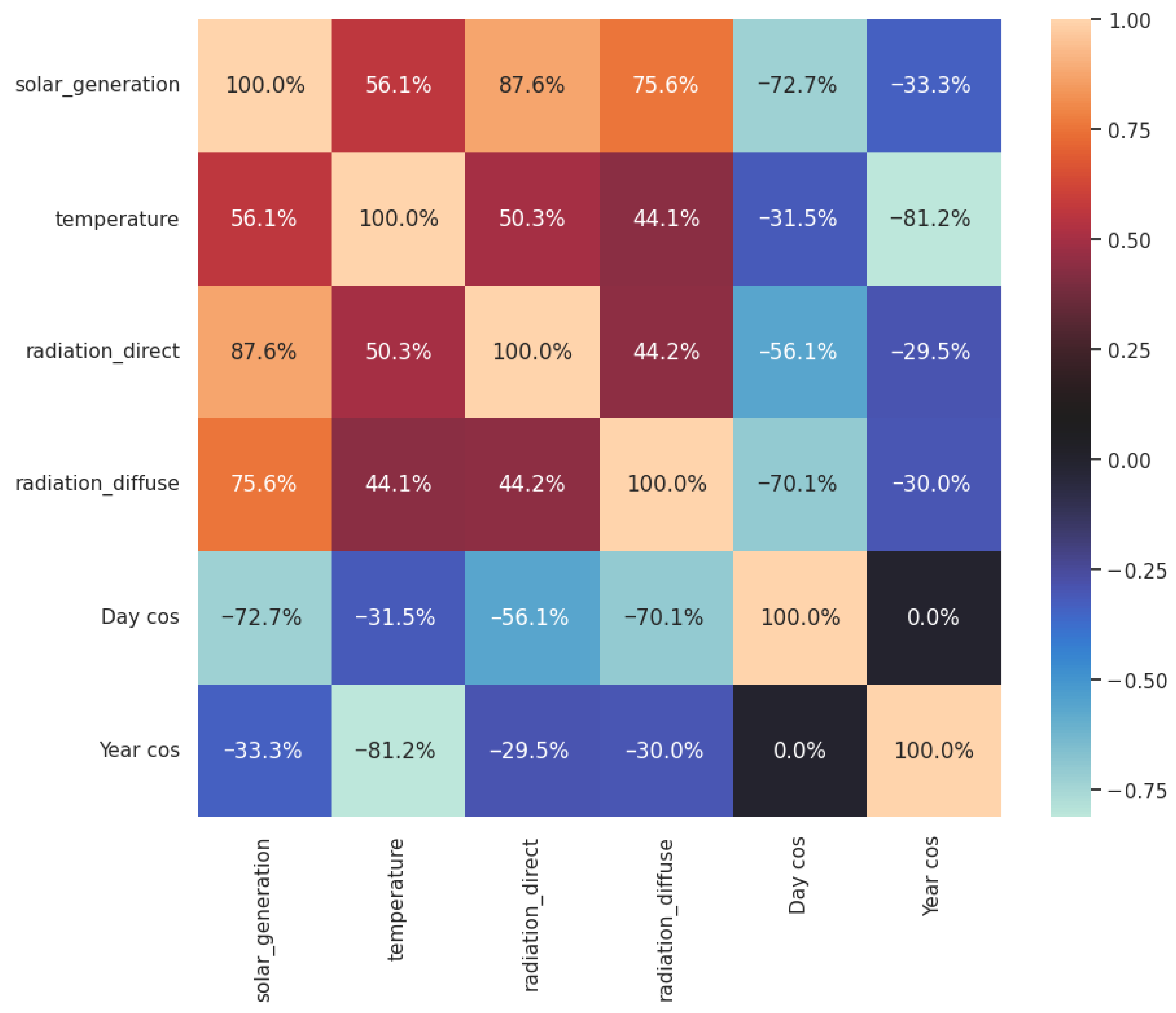
was computed between all pairs of variables in order to determine which variables are highly positive or negatively correlated with the independent variable (i.e., “solar generation”) and between them. The correlation matrix is visualized in Figure 1. Variables highly correlated with the independent variable are the most informative, so they will be selected as inputs for the model. Variables with low correlation and non-significant p-value ($p>0.05$) with the target variable (i.e., “date_time”, “wind_generation”, “Day_sin”, “Year_sin”) were removed. Variables exhibiting high multicollinearity (i.e., “portal_load”, “calculated_load”) were also removed. Removing uncorrelated variables is a common practice in feature engineering in order to reduce model complexity and to improve the efficiency of the learning process [57].

The correlation matrices displayed in Figure 1 (all variables) and Figure 2 (restricted to the selected variables) illustrate the feature selection process. The final feature set retained in Figure 2 includes the most relevant and informative variables: “temperature”, “radiation_direct”, “radiation_diffuse”, “Day_cos”, and “Year_cos”. This selection of variables focuses the model on the key meteorological and cyclical daylight drivers of PV generation, improving efficiency and performance.

3.5. Model Validation

The consolidated database is divided into different sets, considering 70% of the data for training, 20% for validation, and 10% for testing. In order to preserve the temporal information of the data, samples are not randomly reordered or shuffled. Subsequently, the data is normalized by computing the z-scores of each variable independently, excluding the target variable (solar_generation), subtracting its mean, and dividing by its standard deviation, ensuring that the predictive model does not assign greater importance to some features just because, due to their measurement units, they have greater magnitude.

Only training data is used to adjust the normalization scale, preventing data leakage, which occurs when data information outside the training set is accidentally used in model creation, biasing its generalization and prediction capabilities. Therefore, this normalization transformation learned from the training dataset is applied to the validation, and test sets independently.

Time series data is decomposed into sliding windows using a custom class that we call “Window Generator” [58], shown here in pseudo-code as Algorithm 1. Each data window represents a segment of time steps used as inputs to the model, with the corresponding values of the independent variable that the model seeks to predict.

Algorithm 1 Time series sliding window generator

Initialization: (a) Save the training, validation, and test data, which have been previously separated. (b) If labels exist, calculate the indices of their column and those of the rest of the data. (c) Define the window size: input_width, label_width, and shift. (d) Calculate the total window size: total_window_size = input_width + shift. (e) Define input and label indices: i. input_indices = indices from 0 to input_width. ii. label_indices = indices from (total_window_size - label_width) to the end. Window Splitting: (a) Split features (features) into inputs and labels using the defined indices. (b) If there are label columns specified, select corresponding labels. (c) Set up inputs and labels tensors. (d) Return inputs and labels. Generating the dataset: (a) Convert the data to a NumPy array. (b) Create a time series dataset using the total window size (total_window_size) and apply the split_window function. (c) Return the dataset.

3.6. Models

Various regression and neural network techniques were implemented for energy prediction using historical and weather data time series windows as input. Two basic prediction scenarios have been explored: single-step prediction or multi-step prediction, differing in the prediction horizon that can be either one contiguous hour or the next 24 h. The study evaluates traditional ML models and neural network architectures such as Recurrent Neural Network (RNN) and Convolutional Neural Network (CNN).

3.6.1. Baseline

As a comparative baseline, four models were used for both prediction scenarios. The tested models are the following ones, ordered from the simplest to the most complex: the base model, the Linear Regression, the Decision Tree, and the Random Forest. The base model assumes that the next time step will have the same energy generation value as the previous one(s).

3.6.2. One-Step Neural Models

This type of model receives data defined in a sliding input time window, with a defined size, and returns the next single value considering the applied shift.

Linear Perceptron Model

This model differs from linear regression because it is composed of a dense hidden layer with one output neuron, seeking to learn the linear relationships between the selected features and the target variable. This computational architecture is effective for dealing with simple problems where the relationship between the variables is close to or completely linear. The window used for this model contained a time step input, that is, it only takes the most recent data to predict the next one.

Dense Perceptron Model

This Multilayer Perceptron Model (MLP) contains several dense layers, each composed of 64 neurons and using the ReLU activation function. The layer structure is found through a conventional heuristic search. This architecture allows capturing non-linear relationships between variables, including non-linearities, which helps the model to handle more difficult and complicated patterns. As with the linear model, a time step is used as input.

Multiple Input Dense Perceptron Model

This model seeks to modify and expand the scope of the previous one; its architecture includes several dense layers, with the aim of capturing more complex patterns in the data and longer-term trends. This model uses 24 h windows to predict the next hour, allowing the model to learn to make predictions with a greater amount of past information.

Convolutional Neural Network

This CNN-based architecture model uses one-dimensional convolutional layers (Conv1D) with a filter width of 32 to process time sequences. Like the previous model, it receives 24 h time windows as input and, as output, returns the prediction for the next hour.

The CNN architecture is designed to work with gridded data, in which time series are defined over one-dimensional grids [59]. They are characterized by reducing the number of parameters to learn compared to other architectures, which allows for efficient training and increases their ability to capture data patterns that are maintained over a limited period of time [60], making them ideal for real-time applications [59].

Recurrent Neural Network

The RNN model includes an LSTM layer with 32 units, which allows it to remember information from previous steps for a long period, and a final dense layer that computes the output prediction. This architecture is specifically designed to capture long-term dependencies in the data, which is essential when working with complex time series. It is also particularly useful in cases where relationships between data are not immediate but extend across multiple time steps.

3.6.3. Multi-Step Models

Multi-step prediction models use a 24 h window of historical data to predict the next 24 steps (hours) into the future. To achieve this, optimized versions of traditional linear, dense, convolutional, and recurrent models are used. These models are similar to those described above as one-step models but adapted by considering a sequence of 24 steps at a time as the prediction output. In addition, an LSTM-based autoregressive model is incorporated in the comparison.

Baseline Model

The Baseline model does not implement any kind of learning algorithm, i.e., the last value of the input sequence of historical generation values, as it is, is directly used as the predictor for the next value in the output sequence. Its role in the experimental design is to serve as a reference for more advanced models.

Linear Perceptron Model

The Linear model uses the most recent time step in the time window. Its architecture is similar to that of the one-step linear model but optimized to predict multiple future values. It consists of the input layer, a dense layer that produces the predictions, and an output layer that formats the model output properly.

Dense Perceptron Model

This ANN architecture input is the last 24-step window of the data sequence. It has a first hidden dense layer of 512 neurons followed by ReLu activation. The second hidden dense layer of 144 neurons generates the 24 corresponding output predictions. Finally, these results are reorganized in the output layer so that they are displayed properly.

Convolutional Neural Network

The multi-step CNN allows the extraction of local features from the input data, seeking to generate more accurate future predictions, recognizing temporal patterns that are repeated. Its input layer receives the 24-step windows prior to the prediction, followed by a one-dimensional convolutional hidden layer that applies 256 convolutional filters to the sequence, with a kernel of size 24. Next is a dense hidden layer that generates the 24 corresponding predictions to then be reorganized in the output layer to its proper format.

Recurrent Neural Network

The multi-step RNN model is an LSTM architecture. The inputs are a 24-step time windows followed by an LSTM layer with 32 units, whose output passes through a dense hidden, which makes the prediction. Finally, the output layer leaves the result in the appropriate format.

Autoregressive Model

This model predicts one step at a time, but the resulting prediction is re-entered in the model to contribute to the next one-step prediction; this pattern is reproduced throughout the execution of the model. In this way, future predictions are adjusted taking into account previous prediction results. However, errors present in previous predictions can affect the future performance of the model. Finally, LSTM units were used as a base, since they are characterized by capturing long-term temporal dependencies.

4. Results

This section presents the results of the predictive models applied in this work, which are evaluated considering the loss (MSE) and the mean absolute error (MAE) as metrics.

4.1. Results of One-Step Models

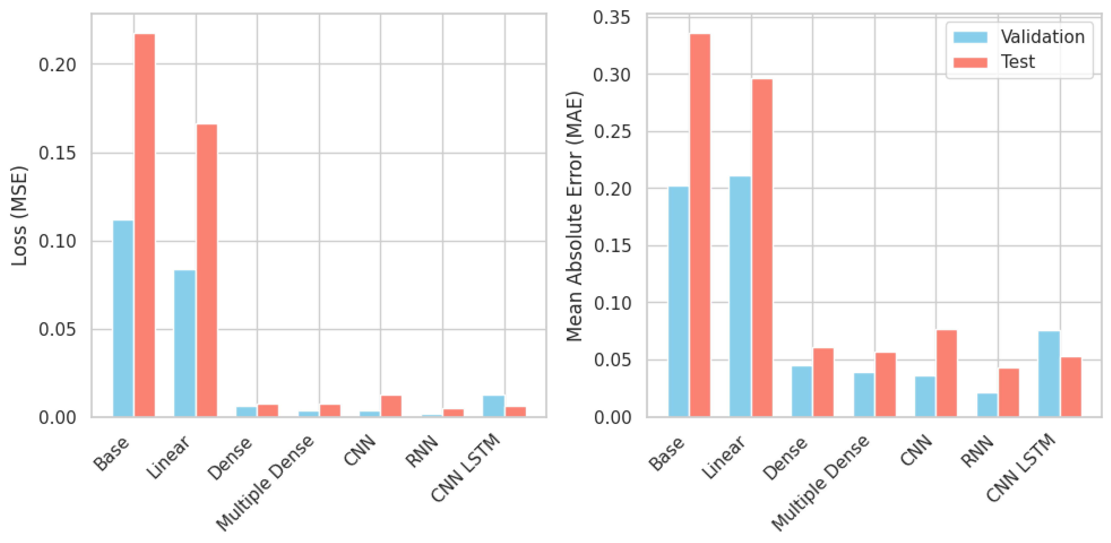
Figure 3 compares five neural network-based models and the reference Base model, i.e., Base, Linear, Dense, Multiple Dense, CNN, and RNN models, showing their performance on both the validation and test sets. It can be seen that the Base model, which is used as a reference, has the highest error values on both sets. The Linear model scarcely improves the Base results, but high MSE and MAE errors are still observed, which suggests that the variables do not have linear relationships with each other. Also, in both models, there are large differences between the validation and test results, which could be indicative of overfitting on the training data.

The dense ANN and CNN-based models have better results than the previous ones, presenting a smaller difference between validation and testing, which suggests that these models have a greater capacity for generalization. Finally, the model that achieves the best results is the RNN-based one, as it shows the lowest value in both error metrics, both for validation and testing.

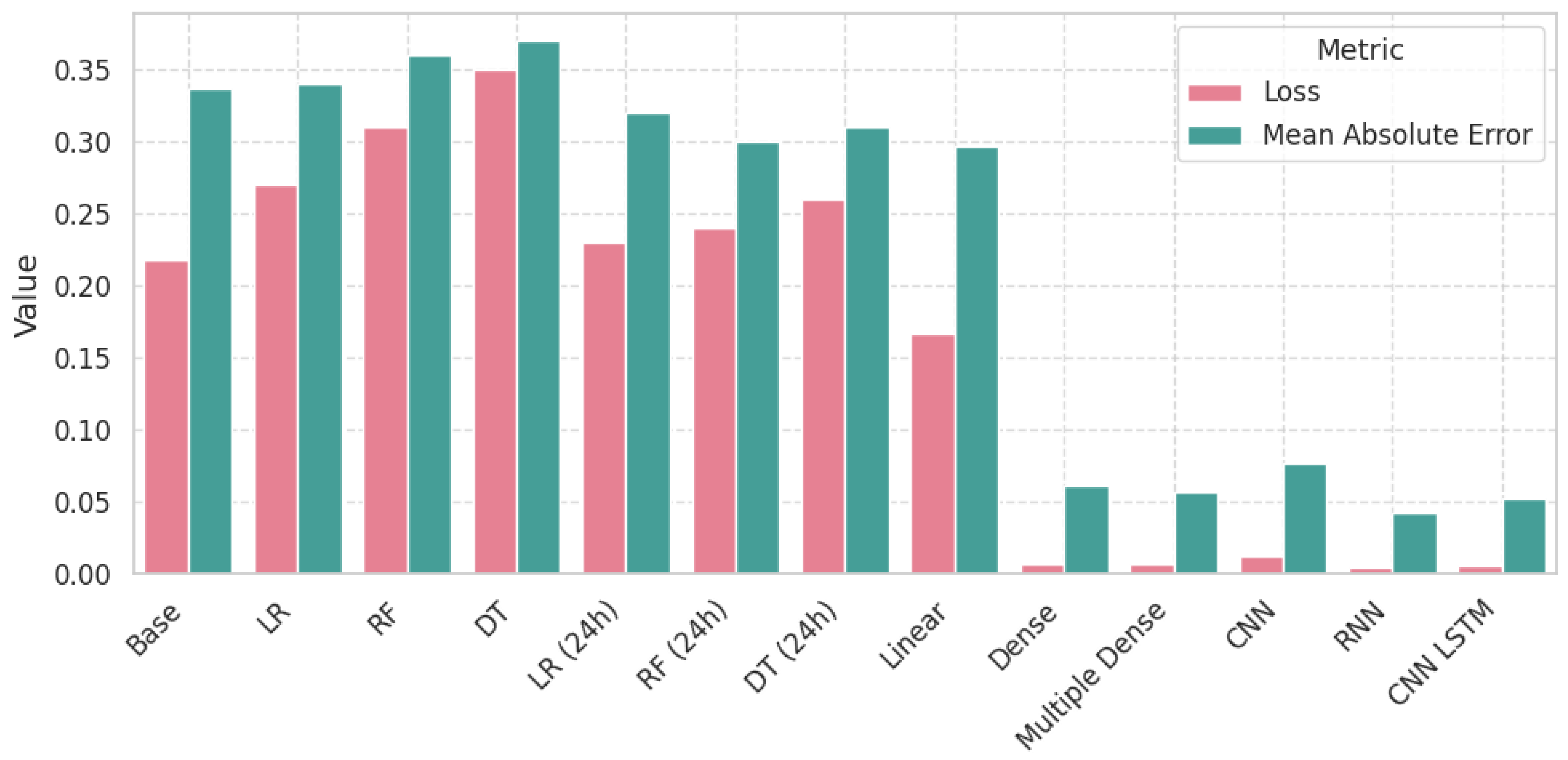
Figure 4 shows detailed results for linear regression (LR), random forest (RF), and decision tree (DT) models and shows the results when using 24 h time windows as the context in them (LR (24 h), RF (24 h), DT (24 h)). It is observed that the more traditional models present higher errors compared to those based on neural networks, considering both metrics. Also, including 24 h time windows as contextual input manages to reduce the prediction error in ML modeling approaches, however not achieving the performance of ANN-based models.

Regarding the ANN models, they clearly show the best comparative performance. Figure 5 shows predictions for sample sliding windows extracted from the test set. The model input (time window) is shown in blue, the real labels in gray, and the model predictions in yellow with a star shape.

4.2. Results of Multi-Step Models

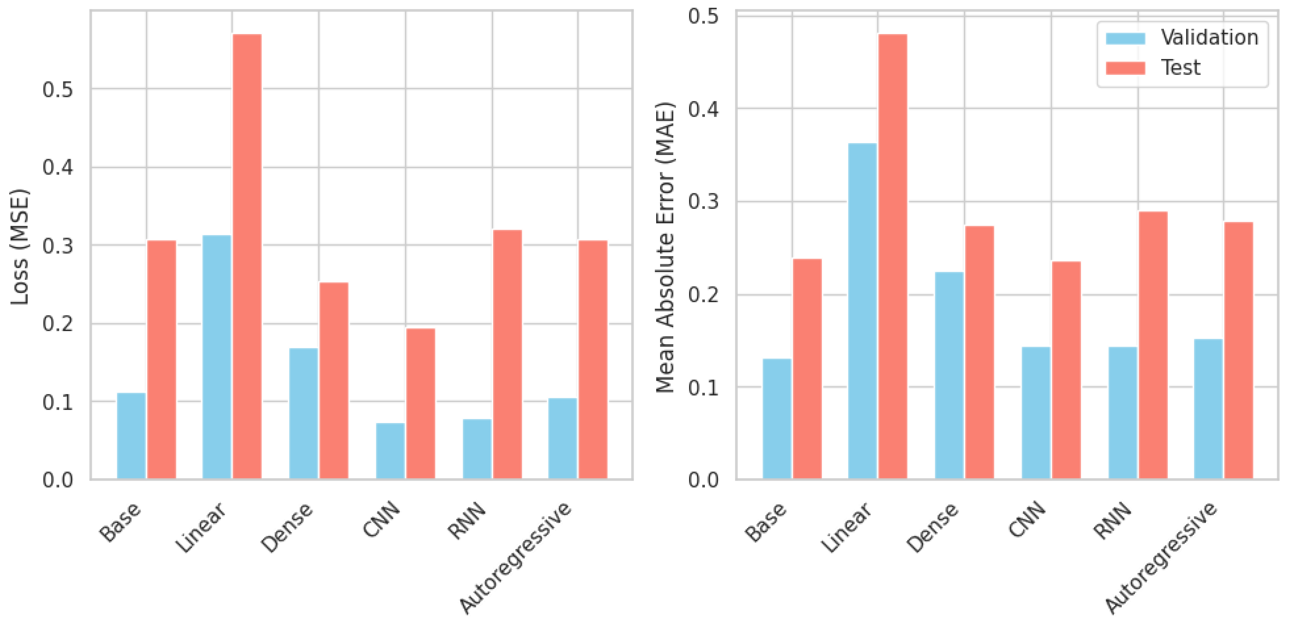
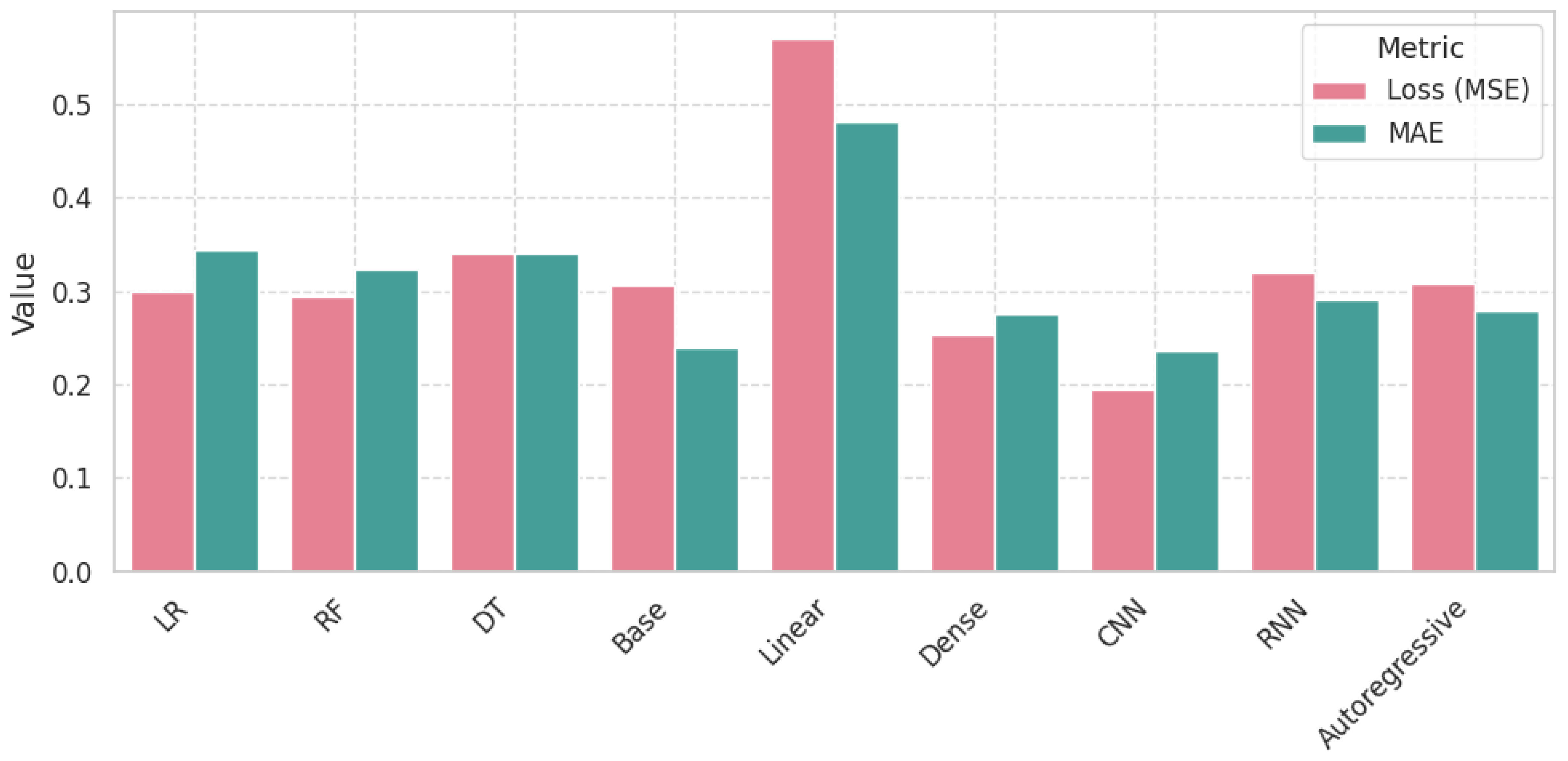
The results obtained for the 24-step (hour) prediction are presented in Figure 6 and Figure 7, comparing the performance of different model architectures both in terms of loss (MSE) and mean absolute error (MAE). The results of traditional models (linear regression (LR), random forests (RF), decision trees (DT)) are included together with those based on neural networks, also considering a hybrid model (Autoregressive model with LSTM modules).

Figure 6 shows the MSE and MAE results of the ANN models over their validation and test sets. The model with the worst results is the Linear model, while the rest of the models show an improvement with respect to these results. The model with the best performance was the CNN architecture.

Figure 7 summarizes the results of all the validated models. The Linear Perceptron model is the one with the worst performance; on the other hand, the CNN model is the one that has the lowest value in both loss and MAE. The rest of the models, both the ML classic ones and those based on ANNs, present similar results, with none standing out prominently over the others.

Figure 8 shows three example windows, providing a qualitative comparison of multi-step forecasts from the CNN and RNN models. It can be seen that the performance differences between both models are rather subtle.

5. Discussion and Conclusions

5.1. Discussion

The analysis of the computational experiments’ results clearly indicates that RNNs, and in particular LSTMs, consistently outperform traditional ML models such as Decision Trees, Linear Regression, and Random Forests in terms of prediction accuracy. The superior performance of LSTMs in single-step and multi-step prediction scenarios can be attributed to their ability to retain long-term dependencies, which is critical when dealing with time series data, such as photovoltaic power generation. This conclusion is in line with the findings of the literature mentioned in the state of the art that highlights the efficiency of LSTMs to capture temporal patterns in complex datasets.

As the results obtained for the LSTM model were satisfactory, its use was expanded using more complex architectures and performing hyperparameter optimization. However, the results reported above were not improved by these more sophisticated approaches. This lack of improvement suggests that the simpler models were already capturing most of the relevant patterns in the data and that the additional model complexities did not bring the expected prediction error reduction.

Convolutional neural networks (CNNs), although initially designed for image recognition, also showed great promise in the context of time series forecasting. Their ability to detect local patterns in the data helped improve predictions, especially in the long term, which was reflected in their superior performance compared to the other architectures in multi-step prediction.

On the other hand, one of the key factors that contributed to the predictive model performance was the inclusion of meteorological data. Solar power generation is highly dependent on environmental conditions such as temperature and solar irradiance. By incorporating these features, the models were able to better anticipate fluctuations in solar power production, which are mainly due to changes in such weather patterns.

In addition, preprocessing the time signal with the sine/cosine transformation significantly helped improve model performance. Representing temporal features, such as time of day or day of year, using these circular transformations allowed models to capture the periodic nature of solar power generation. This signal preprocessing helped the models to generalize across different seasons and times of day, improving the accuracy of short- and long-term forecasts. Without this transformation, the models were unable to uncover recurring seasonal patterns from linear temporal data.

The proposed approach presents several significant advantages. First, the inclusion of cyclical transformations in the temporal variables allows for more accurate capture of the daily and seasonal patterns present in photovoltaic generation, which improves the accuracy of predictions. In addition, the use of a unified pre-processing workflow and the systematic comparison of models under the same experimental conditions provide methodological rigor and reproducibility.

The use of public data and open-source tools promotes transparency and facilitates the replication of experiments. Finally, practical recommendations are offered on what type of neural network to use depending on the prediction horizon (RNN for one-step predictions, CNN for multiple steps), which is valuable for real-world applications.

However, there are also some disadvantages. The performance of the models depends on the availability of clean and complete data, as they were not trained on databases with incomplete or noisy information. Furthermore, models based on deep neural networks require greater computational capacity, which can be an obstacle to their implementation in systems with limited resources.

5.2. Conclusions

In conclusion, the proposed models were able to predict with high accuracy the production of PV energy using available historical values. The results achieved in this work demonstrate the effectiveness of ML models, and specifically deep neural networks for the prediction of photovoltaic energy generation, highlighting RNN architectures as the method with the best results for single-step prediction, and CNNs for multi-step prediction. The integration of meteorological data and circular time features was essential to improve the precision of these models.

Due to the emerging challenge posed by climate change, renewable energies are continuously increasing in socio-economic importance; this is why predictive models, such as those studied in this work, are very useful for improving the management of the electrical grid on the one hand, and, on the other hand, to directly reduce greenhouse gas emissions, especially for the reduction of carbon dioxide emissions by allowing the grid to reduce its dependence on fossil fuels.

The results obtained must be interpreted by taking into account their function as practical tools that provide a useful and replicable approach to improving decision-making in the field of renewable energy generation, its consumption, and possible storage.

This work has demonstrated the potential of deep learning models in photovoltaic energy prediction applications, highlighting the importance of an adequate representation of the data characteristics and the careful consideration of computational costs. In practical implementation, it is important to emphasize the importance of finding an adequate balance between precision and cost when selecting a model for practical field solar energy installations.

5.3. Limitations and Future Work

This study presents several limitations that warrant acknowledgment and future exploration:

• Geographical and Temporal Scope:
  • Validation was conducted exclusively on Austrian data (2015–2017). Generalizability to regions with distinct climatic patterns (e.g., tropical zones with higher irradiance volatility) remains unverified.
  • The dataset excludes extreme weather events (e.g., storms), potentially limiting robustness under anomalous conditions.
• Data Dependency: Model performance relies on high-quality historical data; degradation may occur with noisy or incomplete inputs. Future work will integrate anomaly detection mechanisms to enhance resilience.
• Computational Efficiency: While RNN/CNN architectures achieved high accuracy, their resource demands may hinder deployment in low-infrastructure settings (e.g., edge devices). Simpler models (e.g., Random Forest) could be explored for resource-constrained applications.
• Methodological Refinements: Hyperparameter tuning employed random search, which may yield suboptimal efficiency. Bayesian optimization or evolutionary algorithms will be investigated to accelerate convergence.

Future Directions

• Geographical Transferability: apply transfer learning to adapt models to diverse regions using limited local data.
• Robustness Enhancement: incorporate real-time anomaly detection and data imputation techniques for noisy environments.
• Edge Deployment: develop lightweight model variants (e.g., quantized CNNs) for embedded systems in distributed PV installations.
• Hybrid Physical–AI Modeling: fuse physics-based irradiance models with deep learning to improve extrapolation beyond training conditions.

References

1. U.E.I.A. (EIA). Installed Electricity Capacity. 2022. Available online: https://www.iea.org/reports/renewables-2022 (accessed on 12 July 2024).
2. I.R.E.A. (IRENA). Renewable Energy Statistics 2024. 2024. Available online: https://www.irena.org/Publications/2024/Jul/Renewable-energy-statistics-2024 (accessed on 12 July 2024).
3. I.R.E.A. (IRENA). Renewable Power Generation Costs in 2022. 2023. Available online: https://www.irena.org/Publications/2023/Aug/Renewable-Power-Generation-Costs-in-2022 (accessed on 12 July 2024).
4. Lameirinhas, R.A.M.; Torres, J.P.N.; de Melo Cunha, J.P. A Photovoltaic Technology Review: History, Fundamentals and Applications. Energies 2022, 15, 1823. [Google Scholar] [CrossRef]
5. Charpentier, B.; Cristianetti, R.; Denelle, F.; Dolle, N.; Falcone, G.; Griffiths, C.; Jethwa, D.; Primrose, J.; Seiller, B.; Taupy, J.A.; et al. Specifications for the application of the United Nations Framework Classification for Fossil Energy and Mineral Reserves and Resources 2009 to Renewable Energy Resources; UNECE: Geneva, Switzerland, 2016. [Google Scholar]
6. Wang, M.; Peng, J.; Luo, Y.; Shen, Z.; Yang, H. Comparison of different simplistic prediction models for forecasting PV power output: Assessment with experimental measurements. Energy 2021, 224, 120162. [Google Scholar] [CrossRef]
7. Górriz, J.; Álvarez Illán, I.; Álvarez-Marquina, A.; Arco, J.E.; Atzmueller, M.; Ballarini, F.; Barakova, E.; Bologna, G.; Bonomini, P.; Castellanos-Dominguez, G.; et al. Computational approaches to Explainable Artificial Intelligence: Advances in theory, applications and trends. Inf. Fusion 2023, 100, 101945. [Google Scholar] [CrossRef]
8. Li, L.L.; Wen, S.Y.; Tseng, M.L.; Wang, C.S. Renewable energy prediction: A novel short-term prediction model of photovoltaic output power. J. Clean. Prod. 2019, 228, 359–375. [Google Scholar] [CrossRef]
9. Villemin, T.; Farges, O.; Parent, G.; Claverie, R. Monte Carlo prediction of the energy performance of a photovoltaic panel using detailed meteorological input data. Int. J. Therm. Sci. 2024, 195, 108672. [Google Scholar] [CrossRef]
10. Coelho, S.; Machado, J.; Monteiro, V.; Afonso, J.L. Chapter 11—Power electronics technologies for renewable energy sources. In Recent Advances in Renewable Energy Technologies; Jeguirim, M., Ed.; Academic Press: Cambridge, MA, USA, 2022; pp. 403–455. [Google Scholar] [CrossRef]
11. Mousavi Ajarostaghi, S.S.; Mousavi, S.S. Solar energy conversion technologies: Principles and advancements. In Solar Energy Advancements in Agriculture and Food Production Systems; Elsevier: Amsterdam, The Netherlands, 2022; pp. 29–76. [Google Scholar] [CrossRef]
12. Ghosh, S.; Yadav, R. Future of photovoltaic technologies: A comprehensive review. Sustain. Energy Technol. Assessments 2021, 47, 101410. [Google Scholar] [CrossRef]
13. Peratikou, S.; Charalambides, A.G. Short-term PV energy yield predictions within city neighborhoods for optimum grid management. Energy Build. 2024, 323, 114773. [Google Scholar] [CrossRef]
14. Jha, S.K.; Bilalovic, J.; Jha, A.; Patel, N.; Zhang, H. Renewable energy: Present research and future scope of Artificial Intelligence. Renew. Sustain. Energy Rev. 2017, 77, 297–317. [Google Scholar] [CrossRef]
15. Afridi, Y.; Ahmad, K.; Hassan, L. Artificial Intelligence Based Prognostic Maintenance of Renewable Energy Systems: A Review of Techniques, Challenges, and Future Research Directions. Int. J. Energy Res. 2021, 46, 21619–21642. [Google Scholar] [CrossRef]
16. Yousef, L.A.; Yousef, H.; Rocha-Meneses, L. Artificial Intelligence for Management of Variable Renewable Energy Systems: A Review of Current Status and Future Directions. Energies 2023, 16, 8057. [Google Scholar] [CrossRef]
17. Li, Y.; Janik, P.; Schwarz, H. Prediction and aggregation of regional PV and wind generation based on neural computation and real measurements. Sustain. Energy Technol. Assess. 2023, 57, 103314. [Google Scholar] [CrossRef]
18. Hu, J.; Lim, B.H.; Tian, X.; Wang, K.; Xu, D.; Zhang, F.; Zhang, Y. A Comprehensive Review of Artificial Intelligence Applications in the Photovoltaic Systems. CAAI Artif. Intell. Res. 2024, 3, 9150031. [Google Scholar] [CrossRef]
19. Rezaul Karim, S.; Sarker, D.; Monirul Kabir, M. Analyzing the impact of temperature on PV module surface during electricity generation using machine learning models. Clean. Energy Syst. 2024, 9, 100135. [Google Scholar] [CrossRef]
20. Parenti, M.; Fossa, M.; Delucchi, L. A model for energy predictions and diagnostics of large-scale photovoltaic systems based on electric data and thermal imaging of the PV fields. Renew. Sustain. Energy Rev. 2024, 206, 114858. [Google Scholar] [CrossRef]
21. Tsai, W.C.; Tu, C.S.; Hong, C.M.; Lin, W.M. A Review of State-of-the-Art and Short-Term Forecasting Models for Solar PV Power Generation. Energies 2023, 16, 5436. [Google Scholar] [CrossRef]
22. Chandel, S.S.; Gupta, A.; Chandel, R.; Tajjour, S. Review of deep learning techniques for power generation prediction of industrial solar photovoltaic plants. Sol. Compass 2023, 8, 100061. [Google Scholar] [CrossRef]
23. Quan, R.; Qiu, Z.; Wan, H.; Yang, Z.; Li, X. Dung beetle optimization algorithm-based hybrid deep learning model for ultra-short-term PV power prediction. iScience 2024, 27, 111126. [Google Scholar] [CrossRef] [PubMed]
24. Boza, P.; Evgeniou, T. Artificial Intelligence to Support the Integration of Variable Renewable Energy Sources to the Power System. Appl. Energy 2021, 290, 116754. [Google Scholar] [CrossRef]
25. Raza, M.Q.; Khosravi, A. A Review on Artificial Intelligence Based Load Demand Forecasting Techniques for Smart Grid and Buildings. Renew. Sustain. Energy Rev. 2015, 50, 1352–1372. [Google Scholar] [CrossRef]
26. Shapi, M.K.M.; Ramli, N.A.; Awalin, L.J. Energy Consumption Prediction by Using Machine Learning for Smart Building: Case Study in Malaysia. Dev. Built Environ. 2021, 5, 100037. [Google Scholar] [CrossRef]
27. Ridha, H.M.; Hizam, H.; Mirjalili, S.; Othman, M.L.; Ya’acob, M.E.; Wahab, N.I.B.A.; Ahmadipour, M. A novel prediction of the PV system output current based on integration of optimized hyperparameters of multi-layer neural networks and polynomial regression models. Next Energy 2025, 8, 100256. [Google Scholar] [CrossRef]
28. Wahid, F.; Kim, D. A Prediction Approach for Demand Analysis of Energy Consumption Using K-Nearest Neighbor in Residential Buildings. Int. J. Smart Home 2016, 10, 97–108. [Google Scholar] [CrossRef]
29. Martínez-Álvarez, F.; Troncoso, A.; Riquelme, J.C.; Aguilar-Ruiz, J.S. Energy Time Series Forecasting Based on Pattern Sequence Similarity. IEEE Trans. Knowl. Data Eng. 2011, 23, 1230–1243. [Google Scholar] [CrossRef]
30. Sun, F.; Li, L.; Bian, D.; Ji, H.; Li, N.; Wang, S. Short-term PV power data prediction based on improved FCM with WTEEMD and adaptive weather weights. J. Build. Eng. 2024, 90, 109408. [Google Scholar] [CrossRef]
31. Al-Dahidi, S.; Alrbai, M.; Rinchi, B.; Al-Ghussain, L.; Ayadi, O.; Alahmer, A. A tiered NARX model for forecasting day-ahead energy production in distributed solar PV systems. Clean. Eng. Technol. 2024, 23, 100831. [Google Scholar] [CrossRef]
32. Massidda, L.; Bettio, F.; Marrocu, M. Probabilistic day-ahead prediction of PV generation. A comparative analysis of forecasting methodologies and of the factors influencing accuracy. Sol. Energy 2024, 271, 112422. [Google Scholar] [CrossRef]
33. Dewi, T.; Mardiyati, E.N.; Risma, P.; Oktarina, Y. Hybrid Machine learning models for PV output prediction: Harnessing Random Forest and LSTM-RNN for sustainable energy management in aquaponic system. Energy Convers. Manag. 2025, 330, 119663. [Google Scholar] [CrossRef]
34. Tripathi, A.K.; Aruna, M.; Elumalai, P.; Karthik, K.; Khan, S.A.; Asif, M.; Rao, K.S. Advancing solar PV panel power prediction: A comparative machine learning approach in fluctuating environmental conditions. Case Stud. Therm. Eng. 2024, 59, 104459. [Google Scholar] [CrossRef]
35. Aler, R.; Huertas-Tato, J.; Valls, J.M.; Galván, I.M. Improving Prediction Intervals Using Measured Solar Power with a Multi-Objective Approach. Energies 2019, 12, 4713. [Google Scholar] [CrossRef]
36. Souabi, S.; Chakir, A.; Tabaa, M. Data-driven prediction models of photovoltaic energy for smart grid applications. Energy Rep. 2023, 9, 90–105. [Google Scholar] [CrossRef]
37. Peng, Z.; Peng, S.; Fu, L.; Lu, B.; Tang, J.; Wang, K.; Li, W. A novel deep learning ensemble model with data denoising for short-term wind speed forecasting. Energy Convers. Manag. 2020, 207, 112524. [Google Scholar] [CrossRef]
38. Mousavi, S.M.; Ghasemi, M.; Dehghan Manshadi, M.; Mosavi, A. Deep Learning for Wave Energy Converter Modeling Using Long Short-Term Memory. Mathematics 2021, 9, 871. [Google Scholar] [CrossRef]
39. Chen, Y.; Zhang, D.; Li, X.; Peng, Y.; Wu, C.; Pu, H.; Zhou, D.; Cao, Y.; Zhang, J. Significant Wave Height Prediction through Artificial Intelligent Mode Decomposition for Wave Energy Management. Energy AI 2023, 14, 100257. [Google Scholar] [CrossRef]
40. Aravena-Cifuentes, A.P.; Nuñez-Gonzalez, J.D.; Elola, A.; Ivanova, M. Development of AI-Based Tools for Power Generation Prediction. Computation 2023, 11, 232. [Google Scholar] [CrossRef]
41. Maciel, J.N.; Ledesma, J.J.G.; Junior, O.H.A. Hybrid prediction method of solar irradiance applied to short-term photovoltaic energy generation. Renew. Sustain. Energy Rev. 2024, 192, 114185. [Google Scholar] [CrossRef]
42. Roldán-Blay, C.; Abad-Rodríguez, M.F.; Abad-Giner, V.; Serrano-Guerrero, X. Interval-based solar photovoltaic energy predictions: A single-parameter approach with direct radiation focus. Renew. Energy 2024, 230, 120821. [Google Scholar] [CrossRef]
43. Singh, K.; Mistry, K.D.; Patel, H.G. Optimizing power loss in mesh distribution systems: Gaussian Regression Learner Machine learning-based solar irradiance prediction and distributed generation enhancement with Mono/Bifacial PV modules using Grey Wolf Optimization. Renew. Energy 2024, 237, 121590. [Google Scholar] [CrossRef]
44. Zhang, Z.; Huang, X.; Li, C.; Cheng, F.; Tai, Y. CRAformer: A cross-residual attention transformer for solar irradiation multistep forecasting. Energy 2025, 320, 135214. [Google Scholar] [CrossRef]
45. Li, N.; Li, L.; Huang, F.; Liu, X.; Wang, S. Photovoltaic power prediction method for zero energy consumption buildings based on multi-feature fuzzy clustering and MAOA-ESN. J. Build. Eng. 2023, 75, 106922. [Google Scholar] [CrossRef]
46. Park, J.; Kim, J.; Lee, S.; Choi, J.K. Machine learning based photovoltaic energy prediction scheme by augmentation of on-site IoT data. Future Gener. Comput. Syst. 2022, 134, 1–12. [Google Scholar] [CrossRef]
47. Dai, H.; Zhen, Z.; Wang, F.; Lin, Y.; Xu, F.; Duić, N. A short-term PV power forecasting method based on weather type credibility prediction and multi-model dynamic combination. Energy Convers. Manag. 2025, 326, 119501. [Google Scholar] [CrossRef]
48. Xu, X.; Guan, L.; Wang, Z.; Yao, R.; Guan, X. A double-layer forecasting model for PV power forecasting based on GRU-Informer-SVR and Blending ensemble learning framework. Appl. Soft Comput. 2025, 172, 112768. [Google Scholar] [CrossRef]
49. Li, Y.; Huang, W.; Lou, K.; Zhang, X.; Wan, Q. Short-term PV power prediction based on meteorological similarity days and SSA-BiLSTM. Syst. Soft Comput. 2024, 6, 200084. [Google Scholar] [CrossRef]
50. Markovics, D.; Mayer, M.J. Comparison of machine learning methods for photovoltaic power forecasting based on numerical weather prediction. Renew. Sustain. Energy Rev. 2022, 161, 112364. [Google Scholar] [CrossRef]
51. Zoubir, Z.; Es-sakali, N.; Er-retby, H.; Mghazli, M.O. Prediction of energy production in a building-integrated photovoltaic system using machine learning algorithms. Procedia Comput. Sci. 2024, 236, 75–82. [Google Scholar] [CrossRef]
52. Wiese, F.; Schlecht, I.; Bunke, W.D.; Gerbaulet, C.; Hirth, L.; Jahn, M.; Kunz, F.; Lorenz, C.; Mühlenpfordt, J.; Reimann, J.; et al. Open Power System Data – Frictionless data for electricity system modelling. Appl. Energy 2019, 236, 401–409. [Google Scholar] [CrossRef]
53. Muehlenpfordt, J. Data Package Time Series. 2018. Available online: https://data.open-power-system-data.org/time_series/2018-06-30 (accessed on 12 May 2024).
54. Pfenninger, S.; Staffell, I. Data Package Weather Data. 2018. Available online: https://data.open-power-system-data.org/weather_data/2018-09-04 (accessed on 12 May 2024).
55. Allison, D. How to Encode the Cyclic Properties of Time with Python. 2018. Available online: https://medium.com/@dan.allison/how-to-encode-the-cyclic-properties-of-time-with-python-6f4971d245c0 (accessed on 12 May 2024).
56. Kaleko, D. Feature Engineering–Handling Cyclical Features. 2017. Available online: https://blog.davidkaleko.com/feature-engineering-cyclical-features.html (accessed on 12 May 2024).
57. Zheng, A.; Casari, A. Feature Engineering for Machine Learning: Principles and Techniques for Data Scientists; O’Reilly Media: Sebastopol, CA, USA, 2018. [Google Scholar]
58. Abadi, M.; Agarwal, A.; Barham, P.; Brevdo, E.; Chen, Z.; Citro, C.; Corrado, G.S.; Davis, A.; Dean, J.; Devin, M.; et al. TensorFlow: Large-Scale Machine Learning on Heterogeneous Systems. 2015. Available online: http://tensorflow.org/ (accessed on 12 May 2024).
59. Amarasinghe, K.; Marino, D.L.; Manic, M. Deep neural networks for energy load forecasting. In Proceedings of the 2017 IEEE 26th International Symposium on Industrial Electronics (ISIE), Edinburgh, UK, 19–21 June 2017; pp. 1483–1488. [Google Scholar] [CrossRef]
60. Sadouk, L. CNN approaches for time series classification. Time Ser. Anal.-Data Methods Appl. 2019, 5, 57–78. [Google Scholar]
Figure 1. Correlation matrix between all variables contained in the database.
Electronics 14 04263 g001
Figure 2. Correlation matrix between the variables selected for training the predictive models.
Electronics 14 04263 g002
Figure 3. MSE and MAE results of one-step models based on neural networks.
Electronics 14 04263 g003
Figure 4. Comparative results of one-step models.
Electronics 14 04263 g004
Figure 5. Window examples of the solar generation one-step ahead predictions achieved by the RNN optimal model. (a) Example window 1. (b) Example window 2. (c) Example window 3.
Electronics 14 04263 g005
Figure 6. Comparative MSE and MAE results of multi-step models based on neural networks.
Electronics 14 04263 g006
Figure 7. Comparative MSE and MAE results of multi-step models including ML approaches.
Electronics 14 04263 g007
Figure 8. Sample windows for solar generation multi-step predictions by the two best neural network-based models, namely CNN and RNN. (a) CNN predictions. Example window 1. (b) RNN predictions. Example window 1. (c) CNN predictions. Example window 2. (d) RNN predictions. Example window 2. (e) CNN predictions. Example window 3. (f) RNN predictions. Example window 3.
Electronics 14 04263 g008
Disclaimer/Publisher’s Note: The statements, opinions and data contained in all publications are solely those of the individual author(s) and contributor(s) and not of MDPI and/or the editor(s). MDPI and/or the editor(s) disclaim responsibility for any injury to people or property resulting from any ideas, methods, instructions or products referred to in the content.