Article

A Novel Gating Adversarial Imputation Method for High-Fidelity Restoration of Missing Electrical Disturbance Data

by
Lidan Chen
1,
Guangxu Feng
2,* and
Lei Wang
1,*
1
School of Shipping and Maritime Studies, Guangzhou Maritime University, Guangzhou 510725, China
2
State Key Laboratory of Internet of Things for Smart City and Department of Electrical and Computer Engineering, University of Macau, Macau, China
*
Authors to whom correspondence should be addressed.
Electronics 2025, 14(20), 4108; https://doi.org/10.3390/electronics14204108
Submission received: 19 July 2025 / Revised: 13 October 2025 / Accepted: 17 October 2025 / Published: 20 October 2025
(This article belongs to the Special Issue Cyber-Physical System Applications in Smart Power and Microgrids)

Abstract

The ongoing evolution of cyber-physical power systems renders them susceptible to frequent and multifaceted electrical disturbances. Critically, missingness resulting from cascading cyber-physical failures severely impedes the ability to accurately monitor and diagnose these electrical disturbances. To address this serious challenge, this paper proposes a novel gating adversarial imputation (GAI) framework specially tailored for the high-fidelity restoration of missing electrical disturbance data. The proposed GAI efficiently introduces the latest gating mechanism into a stability-improved adversarial imputation process, enabling robust feature representation while maintaining high imputation accuracy. To validate its efficacy, a synthetic dataset encompassing 15 distinct disturbance types is constructed based on precise mathematical equations and standard missingness. A comprehensive experimental evaluation demonstrates that the proposed GAI consistently outperforms five representative imputation benchmarks across all tested missing percentages. Moreover, GAI effectively preserves the original critical characteristics during data recovery, thereby enhancing accurate system monitoring and operational security.

1. Introduction

Modern electrical grids are undergoing a paradigm shift towards complex cyber-physical power systems (CPPSs) [1]. The tremendous transformation is driven by the need to accommodate a massive influx of distributed energy resources (DERs), optimize daily operational efficiency, and improve the whole system’s reliability [2]. Fulfilling these requirements requires the deep integration of advanced information and communication technologies, such as phasor measurement units (PMUs) and wide-area monitoring systems (WAMS), into the physical and electrical infrastructure [3].
The rapid development of WAMS offers a comprehensive and real-time snapshot of power system states, thus significantly improving monitoring efficiency [4]. Its success relies on two critical conditions. Firstly, complete observability is achieved through optimal placement so that system states can be fully reconstructed from PMU measurements [5]. Secondly, the communication network in WAMS must possess adequate channel capacity to reliably transmit high-resolution data from PMUs to phasor data concentrators (PDCs) [6] under strict bandwidth and latency constraints. This limitation on channel capacity becomes paramount for timely system response to fast-developing electrical transients [7].
Concurrently, the intricate coupling of cyber and physical components, compounded by the proliferation of inverter-based resources, nonlinear loads, and grid automation, has fundamentally altered electrical characteristics [8]. In addition, as system operations become more dynamic due to DER penetration, shifting load patterns, topology changes, and other uncertainties, the system becomes increasingly complex and harder to monitor and control [9]. As a consequence, this renders the CPPS highly susceptible to frequent and multifaceted electrical disturbances. More specifically, electrical disturbances, namely, power quality disturbances (PQDs), encompassing voltage sags, swells, harmonics, various transients, and frequency fluctuations, pose a severe threat to system reliability.
Under these more complex and less predictable operating conditions, the consequences of electrical disturbances are amplified, spanning from triggering equipment malfunctions, causing huge economic losses, and even cascading into widespread blackouts [10]. These evolving conditions increase the risk that a localized cyber or physical disturbance will propagate, triggering widespread failures across the cyber-physical infrastructure. Hence, accurate and efficient monitoring on these electrical disturbances is critical to the secure operation of CPPS.
The efficacy of the disturbance monitoring systems is fundamentally dependent on the acquisition of complete and high-fidelity measurements [11]. However, data integrity challenges, especially missingness, frequently stem from various cyber-physical failures, such as measurement sensor faults [12], communication failure, and data manipulation attacks [13]. The prevalence of missing data severely compromises the CPPS monitoring capabilities, resulting in the misidentification or omission of critical disturbance events, causing erroneous state estimations, and undermining the efficacy of data-driven control algorithms [14]. Together, these deficiencies constitute a direct threat to the operational security of a system.
Within the monitoring scenarios of CPPS, data missingness among electrical disturbances concretely manifests as missing values in crucial PMU measurement streams. According to the reports of system operators at China Southern Power Grid, approximately 10% to 30% of PMU measurements are affected by missing issues during daily operations [15]. Here, we detail common factors causing missing PMU data. Even under some particular circumstances, cyberattacks lead to missingness on purpose [16]. For example, the global positioning system (GPS) spoofing attack in [16] renders PMU measurements of the specific temporal or spatial index inaccurate or even unusable. But there is no publicly available incident reports regarding missingness events by cyberattacks. Synchrophasor communication failures and device malfunctions constitute the main causes of missing PMU data. The relevant issues are mentioned in [14,15,17]. The majority of existing studies do not benchmark against realistic data missingness patterns, typically simulating missingness through the random deletion of data points. In particular, in [15], only real-world PMU measurements of Guangdong power grid are tested, and this dataset contains real missing data. Notably, this reveals that the simulated missingness and original missingness are comparable according to the results.
The prevailing works for handling missing data typically assume that the underlying missingness mechanism is either missing completely at random (MCAR) or missing at random (MAR). Therein, MCAR is preferred and widely used in generating missing PMU data artificially, such as [15,17], etc. For example, to simulate missingness in [17], a  1 6 -second data segment is deliberately removed from a randomly selected 10% of PMUs. This removal is specifically timed to coincide with the peak of each 2 s event. All peak data points have a equal chance of being removed. The missing percentage is around 8.33% for each missing PMU.
To deal with missing measurement data, various data imputation strategies have been proposed in the literature. Conventional statistical methods, including mean imputation and forward fill, are computationally simple but largely ineffective for the highly dynamic, subtle, and non-linear waveform characteristics of disturbance signals, often introducing huge bias and distortion [18]. An improvement is provided by traditional machine learning imputation methods, such as random forest (RF) imputation, which can exploit the inherent correlations within a dataset to generate more accurate and contextually plausible estimates [19]. However, these models may still struggle to represent the underlying data distribution, particularly for intricate temporal and distinct disturbance characteristics. To overcome these limitations, the focus has increasingly concentrated on generative adversarial networks (GANs). A representative work in this area is the generative adversarial imputation net (GAIN) algorithm [20], which utilizes a generator to produce missing values and a discriminator to distinguish between generated and observed parts, thus constraining the generator to learn the underlying distribution [21]. While effective, basic GAN architectures are faced with significant training instability issues [22]. This has facilitated the emergence of advanced and domain-specific architectures like SolarGAN [23], which is a Wasserstein GAN (WGAN) variant engineered to enhance training stability and accuracy for time-series data. Despite these advancements, existing methods still struggle to achieve both the high-fidelity restoration of subtle disturbance characteristics and robust imputation performance.
In order to address the critical challenge, this paper introduces a novel gating adversarial imputation (GAI) framework. Central to the proposed methodology is a dynamic gating architecture [24] that operates on a principle analogous to the self-attention mechanism. The integration of this gating mechanism endows our model with the unique capability to preserve and restore the high-fidelity characteristics of disturbance signals. Furthermore, adversarial imputation loss is rigorously constrained, thereby ensuring a consistent and convergent learning process. A comprehensive experimental evaluation demonstrates that the proposed GAI excels at preserving critical disturbance characteristics while maintaining high imputation accuracy.
This research contributes to the field in the following key aspects:
1.
First of all, an innovative GAI framework is proposed for the high-fidelity restoration of missing electrical disturbance data.
2.
The critical introduction of a gating architecture significantly enhances imputation robustness and feature representation, preserving critical original characteristics.
3.
A refined experimental environment is carefully designed using a high-quality disturbance dataset with standard missingness.
4.
Imputation training’s stability is maintained by applying a strict clipping on the adversarial imputation loss.
The remaining sections are briefly described here. The problem formulation of missing electrical disturbances is outlined in Section 2. Then, the architecture and underlying mechanisms of the proposed GAI method are detailed in Section 3. Next, Section 4 presents a comprehensive experimental verification with a high-quality disturbance dataset and state-of-the-art benchmarks. This paper concludes in Section 5 with a brief summary and discussion of future research directions.

2. Problem Formulation

This section offers a theoretical problem formulation of electrical disturbances and the relevant data missingness. Firstly, rigorous mathematical models about different types of disturbances are presented. Subsequently, the core challenge of missing data issues among electrical disturbances is defined and characterized.

2.1. Electrical Disturbance Modeling

Electrical disturbances, also known as power quality disturbances (PQDs), typically refer to anomalous deviations among voltages or currents from a normal electrical power supply [25]. These disturbances severely damage the lifespan of electrical devices and the operation efficiency of power systems. Therein, voltage disturbances are seen as the most common power quality issues [26].
In the settings used for this study, a normal voltage waveform is formulated as follows:
V ( t ) = A [ 1 ± α ( u ( t t 1 ) u ( t t 2 ) ) ] s i n ( w t ) , α 0.1 ,   T t 2 t 1 9 T
where A denotes the maximum voltage magnitude, and α controls voltage magnitude variations below 0.1. u ( t ) represents the step function, and T = 0.02 s is the signal period. t 1 and t 2 adjust the variation duration that varies between T and 9 T . In addition, w = 2 π T refers to the angular frequency. Unlike the previous ideal settings of normal signals in [27,28], the formulation in (1) explicitly accommodates minor fluctuations within normal voltage waveforms. In addition, exactly replicated signals are rare in real-world operations owing to system noise and environmental perturbations.
In general, electrical disturbances can be categorized according to the relevant waveform characteristics, duration, frequency, and amplitude. Following the guidance of the IEEE Standard-1159 [29], apart from normal signals, 15 types of electrical disturbances are characterized and defined on the basis of the precise parametric equations from [11]. All disturbance types are demonstrated in Table 1, and the relevant parametric equations are displayed in Figure 1. For instance, the parametric equation of interruption is written as follows:
V ( t ) = A [ 1 α ( u ( t t 1 ) u ( t t 2 ) ) ] s i n ( w t ) , 0.9 α 1 , T t 2 t 1 9 T
where α adjusts a notable magnitude change between 0.1 and 0.9.
To model the characteristics of real electrical disturbances under complicated cyber-physical power system environments, single and composite disturbance types are incorporated. More specifically, there are seven single disturbances, five double disturbances, and three triple disturbances. In the way, + denotes signal synthesis here. The established models are parameterized based on matching physical characteristics. For duration-based events such as sag, swell, and interruption, α and u ( t ) are utilized to precisely adjust the magnitude and duration of the deviation. While for transient phenomena, including impulsive transients, oscillatory transients, and spikes, a dedicated parameter K controls the peak amplitude. Separately, β f governs the frequency modulation for Flicker.
The process of generating electrical disturbance datasets follows a structured synthesis protocol based on the aforementioned mathematical parametric equations. In the way, a detailed description of step-by-step implementation is demonstrated in Section 4.1.1.
A prominent feature of this algorithm is its explicit handling of fragment selection to prevent repetition, a measure taken to maximize the diversity and realism of the resulting dataset.

2.2. Missingness in Disturbance Data

Missingness issues in electrical disturbance data are described here. Data integrity in the PMU measurements is of paramount importance to the reliable analysis of disturbances. However, missing phenomena are prevalent within these time-series measurements. To develop and validate countermeasures for handling such data gaps, it is essential to understand the underlying mechanism of missingness issues.
In the field of statistics, these issues are systematically categorized into three principal mechanisms of data missingness, including MCAR, MAR, and missing not at random (MNAR) [30]. Their corresponding descriptions are outlined as follows:
  • MAR: This holds if the probability of a missing entry is conditional only upon the observed information and independent of the unobserved missing values [31,32].
  • MCAR: This holds when the missing probability is entirely independent of both observed and unobserved variables [33]. This indicates that missingness occurs as a purely stochastic process, with every data point having an equal and constant probability of being absent.
  • MNAR: This occurs when the missing probability of a value is dependent on the unobserved data itself [34]. In this case, a non-ignorable selection bias is introduced, which cannot be corrected without explicitly modeling the missingness process.
In most real-world applications, the missingness mechanism is assumed to be either MAR or MCAR because the presence of MNAR requires strong and impractical assumptions about the relationship between missing values and missing probabilities. This is because, in real daily operations of modern power systems, the occurrence of missing PMU data events tends to be random, and the missingness mechanism is unknown, so MAR or MCAR is preferred here.
The input electrical disturbance data containing missing values is expressed as the vector V o . To formally identify and intuitively demonstrate the positions of these missingness values, a binary mask M is introduced. The elements of M are set to 1 if the corresponding value in V o is missing, and it is 0 otherwise:
M i j = 1 if V o i j i s N a N 0 if V o i j i s n o t N a N
The mathematical modeling of MAR can be expressed using the following formula:
P ( M = 1 V o , ξ ) = P ( M = 1 V obs , ξ ) ,
where ξ denotes the dependency relation, and V o = ( V obs , V miss ) and V obs refer to the non-missing observed data. Usually, it is assumed that the missingness relation has a linear logistic relationship ξ = W with the observed data V obs . This can be expressed as follows:
ξ = W · V obs ,
where parameters of W are random numbers.
For the missingness analysis of electrical disturbance data from PMUs, the assumption of MCAR is both realistic and methodologically sound [20,21]. As the occurrence of missingness usually results from random power system events, the probability of missing data is independent of measurements. This characteristic is in agreement with the MCAR assumption. Its corresponding mathematical expression is
P ( M = 1 V o , ξ ) = P ( M = 1 ξ )
where this condition reveals that missingness shows no information about the data values, thereby imposing no systematic bias during data recovery. In addition, MCAR is frequently adopted in power system analytics as a foundational assumption for generating synthetic missing data [15,17,35].
As a consequence, MCAR is preferred here to simulate missingness artificially so that the experimental scenarios closely approximate real-life settings, enabling a credible assessment of the imputation algorithm.

3. Proposed Gating Adversarial Imputation

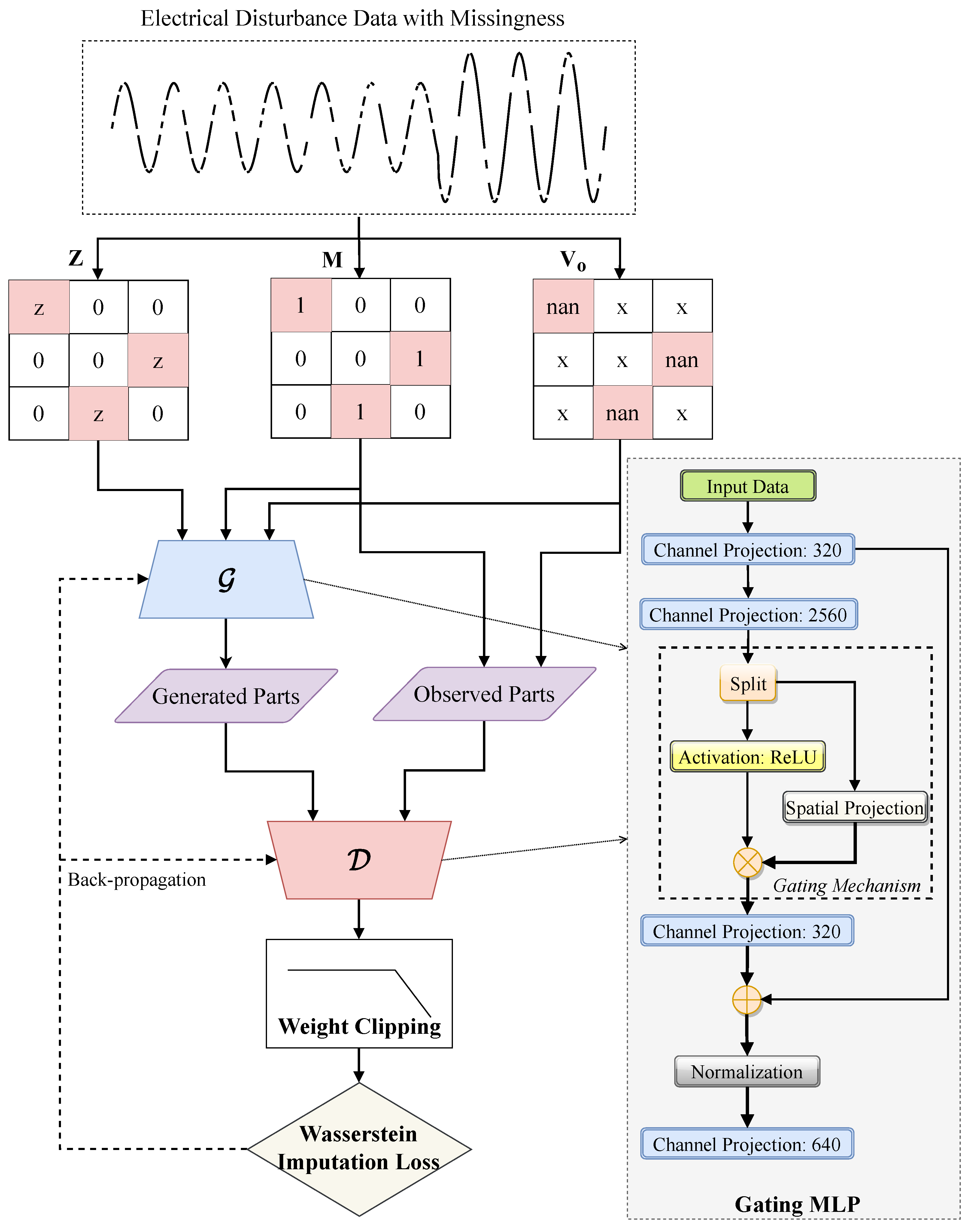
This section introduces the methodology of the proposed gating adversarial imputation, specifically designed to address the issues of missing disturbance data. The general flowchart of the proposed methodology is displayed in Figure 2. It uniquely consists of a gating mechanism and an improved adversarial imputation framework. The gating mechanism provides powerful feature representation capabilities for the adversarial imputation process. Moreover, improved adversarial imputation ensures inherent training stability and robust imputation feature preservation.

3.1. Gating Mechanism

The gating MLP structure proposed by [24] offers an approximating alternative to lite transformers. To model intricate feature dependencies, it leverages channel projections in conjunction with spatial projections modulated by the gating mechanism. As shown in Figure 2, first of all, the input disturbance vector V in is processed by two channel projection layers. The initial layer performs dimensionality reduction for computational efficiency. And the second layer expands the feature dimension, preparing the vector for the split operation essential for the gating mechanism that models spatial interactions. The output X through the initial two projection layers is expressed as
X = F θ 2 F θ 1 ( V in )
where F θ 1 and F θ 2 denote the projection functions parameterized by θ 1 and θ 2 . To implement the gating mechanism, X is split into two intermediate representations, X 1 and X 2 , for processing in two parallel branches. In the branch of X 1 , it undergoes the activation function σ . Concurrently, the second branch applies a spatial projection to X 2 to capture cross-token dependencies. The gating mechanism is subsequently realized by the element-wise multiplication of the outputs from these two branches:
G ( X ) = σ ( X 1 ) S ( X 2 )
where G ( X ) is the gated output, and ⊙ denotes the element-wise Hadamard product. In addition, S ( · ) represents the spatial projection function. Following the gating mechanism, the resulting vector G ( X ) is processed by the projection layer F θ 3 to restore its dimensionality to match the output after the first projection. Through the classic residual connection, the resulting output X ¯ is written as
X ¯ = F θ 3 ( G ( X ) ) + F θ 1 ( V in )
Finally, a separate projection layer F θ 4 is employed to transform the vector X ¯ to the original input dimension. The final output V out is formulated as
V out = F θ 4 ( X ¯ )
Note that the normalization operation has been omitted for clarity in this description.

3.2. Improved Adversarial Imputation

The gating MLP architecture, as detailed in the previous subsection, forms the foundational building blocks for our proposed adversarial imputation methodology. The adversarial imputation framework typically consists of the discriminator D and the generator G . Therein, G is utilized to generate realistic imputation values for missing data points, and D is trained to distinguish between observed complete and generated data pairs. In particular, both D and G are built on the aforementioned gating MLP structures, endowing them with the capacity for efficient feature representation.
As G requires a complete vector as input, V g is constructed by substituting the missing parts in V o with random vector Z from a uniform distribution. The data input portion of G is formulated as
V g = M Z + ( 1 M ) V o
where the whole input to G is expressed as the concatenation [ V g , 1 M ] .
Then, D serves as an adversarial critic to discriminate between the observed complete data and the generated output of G . The disturbance data input to D is formulated as
V d = M G ( [ V g , 1 M ] ) + ( 1 M ) V o
where G ( [ V g , M ] ) is the generated output of G . Different from the standard GAIN algorithm, the hint mechanism is excluded here to compel D to learn intrinsic data dependencies more deeply while also mitigating computation burden. As a consequence, D receives the imputed vector V d as the sole input, enabling a more robust assessment of imputation quality. Wasserstein discrimination loss is adopted for training D , which aims to minimize the difference between observed and generated data [11]. The relevant loss of D is formulated as
L D = E ( 1 M ) D ( V d ) E ( 1 M ) D ( G ( V g , 1 M ) )
where the discrimination output pairs ( 1 M ) D ( V d ) and ( 1 M ) D ( G ( V g , 1 M ) ) in the position of the observed parts are utilized to measure loss.
To mitigate instability issues during adversarial training, such as gradient vanishing, weight clipping is imposed on the parameter space of D [22]. It constrains all parameters of D to remain within in a compact range [ δ , δ ] during the whole training process, thereby enforcing a strict 1-Lipschitz constraint [36]. Weight clipping is formulated as
Θ D δ .
where the clipping operation is applied immediately after each gradient update.
In the subsequent training phase, the parameter G is tuned under the adversarial guidance of D . In the way, the parameters of D are fixed here. The generation loss L GEN is built exclusively from the discrimination output corresponding to the generated data points. It is written as
L GEN = E M D ( V d ) .
By the gradient backpropagation of L GEN , Θ G is updated to generate imputation values that are more likely to be judged as real by D . However, depending merely on the generation loss results in a severe problem, G may tend to generate plausible imputation values that easily fool D yet deviates greatly from the ground truth. To tackle this issue, the mean squared error (MSE) loss, namely, reconstruction loss, is introduced and works as an efficient regularization term. It directly penalizes the distance between the generated and originally observed data, thus ensuring that G preserves the underlying characteristics of the observed parts. The formulation for this MSE loss is displayed as follows:
L MSE = E ( 1 M ) V o ( 1 M ) G ( [ V g , 1 M ] ) 2 .
By a combination of (15) and (16), the overall loss of G is actually a weighted sum of the generation and reconstruction loss terms. The loss L G is formulated as
L G = L GEN + γ L MSE = E M D ( V d ) + γ E ( 1 M ) V o ( 1 M ) G ( [ V g , 1 M ] ) 2 .
where γ denotes the trade-off coefficient between L GEN and L MSE .
Once the adversarial imputation training process is over, meaning that L D and L G have converged, the eventual imputed disturbance data V * can be written as follows:
V * = M G * ( [ V g , 1 M ] ) + ( 1 M ) V o
where G * represents the optimal generator model.
In general, the training procedures of the proposed gating adversarial imputation algorithm is demonstrated in Algorithm 1. The outer while loop, which is set to run for a fixed number of N epochs, contains an inner for loop that runs for K iterations. Inside these loops, the algorithm performs matrix operations and the forward and backward passes of G and D .
Algorithm 1 Proposed Gating Adversarial Imputation Algorithm
  • Input: Disturbance data with missing values V o , random variables Z , clipping factor δ , tuning factor γ , training epochs N learning rate η , critic iterations K
  • Output: Recovered disturbance data V *
  1:
Construct D , G as gating MLP models Θ D , Θ G
  2:
while the adversarial imputation training is not over do
  3:
   for  e p o c h = 1 to N do
  4:
       Derive missingness mask M from V o
  5:
       Input of G : V g M Z + ( 1 M ) V o
  6:
       Input of D : V d M G ( [ V g , 1 M ] ) + ( 1 M ) V o
  7:
       Loss of D : L D E ( 1 M ) D ( V d ) E ( 1 M ) D ( G ( V g , 1 M ) )
  8:
       Weight clipping: Θ D c l i p p i n g ( Θ D , δ , δ )
  9:
        Θ D Θ D + η D [ L D ( 1 M , V g , V d ) ]
10:
     for  i t e r a t i o n = 1 , , K  do
11:
          Generation loss: L GEN E M D ( V d )
12:
          MSE loss: L MSE E ( 1 M ) V o ( 1 M ) G ( [ V g , 1 M ] ) 2
13:
          Loss of G : L G L GEN + γ L MSE
14:
           Θ G Θ G η G [ L G ]
15:
     end for
16:
   end for
17:
end while
18:
Recovered data V * = M G * ( [ V g , 1 M ] ) + ( 1 M ) V o

4. Experiments and Results

This section is divided into two parts: experimental settings and results. First, the procedures for data generation and the overall experimental configuration are described. Following this, the performance of the proposed imputation method is validated and analyzed.

4.1. Experimental Settings

4.1.1. Disturbance Data Generation

First of all, disturbance data generation is introduced. The steps of the electrical disturbance generation process are detailed as follows:
Step 1:
Assign basic constant parameters like the normalized amplitude A = 1 , fundamental frequency f = 50 Hz, and fundamental angular frequency ω = 100 π ; then, define the array of parametric equations with random parameters.
Step 2:
Initialize the disturbance output array V k with a 16 × 641 -shaped zero array. Here, 16 is the number of disturbance types, and 641 is the sum of signal length 640 and its corresponding label length 1.
Step 3:
For each iteration k, a different random seed s e e d ( k ) is set for array V k .
Step 4:
For each disturbance type l a b e l , run the parametric equation F ED ( l a b e l ) . Then, assign it with l a b e l into the corresponding array V l a b e l k .
Step 5:
For each iteration k, output an array V k and stack all V k together into the dataset V .
Step 6:
Shuffle the generated dataset V in random order. The total shape of V is ( 20 · i t e r a t i o n s ) × 641 .
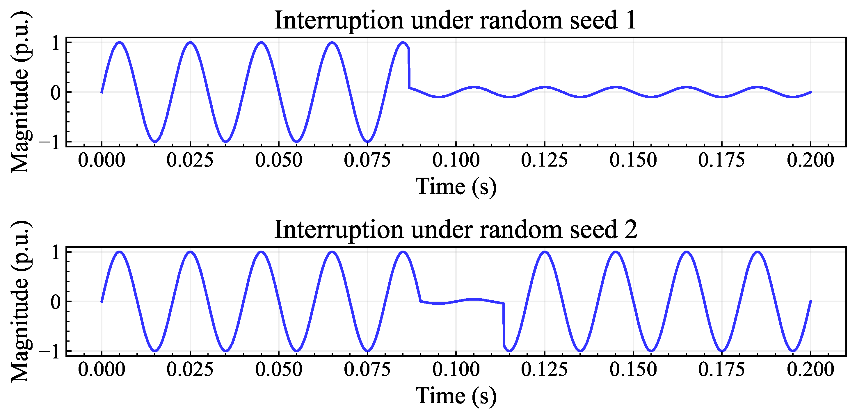
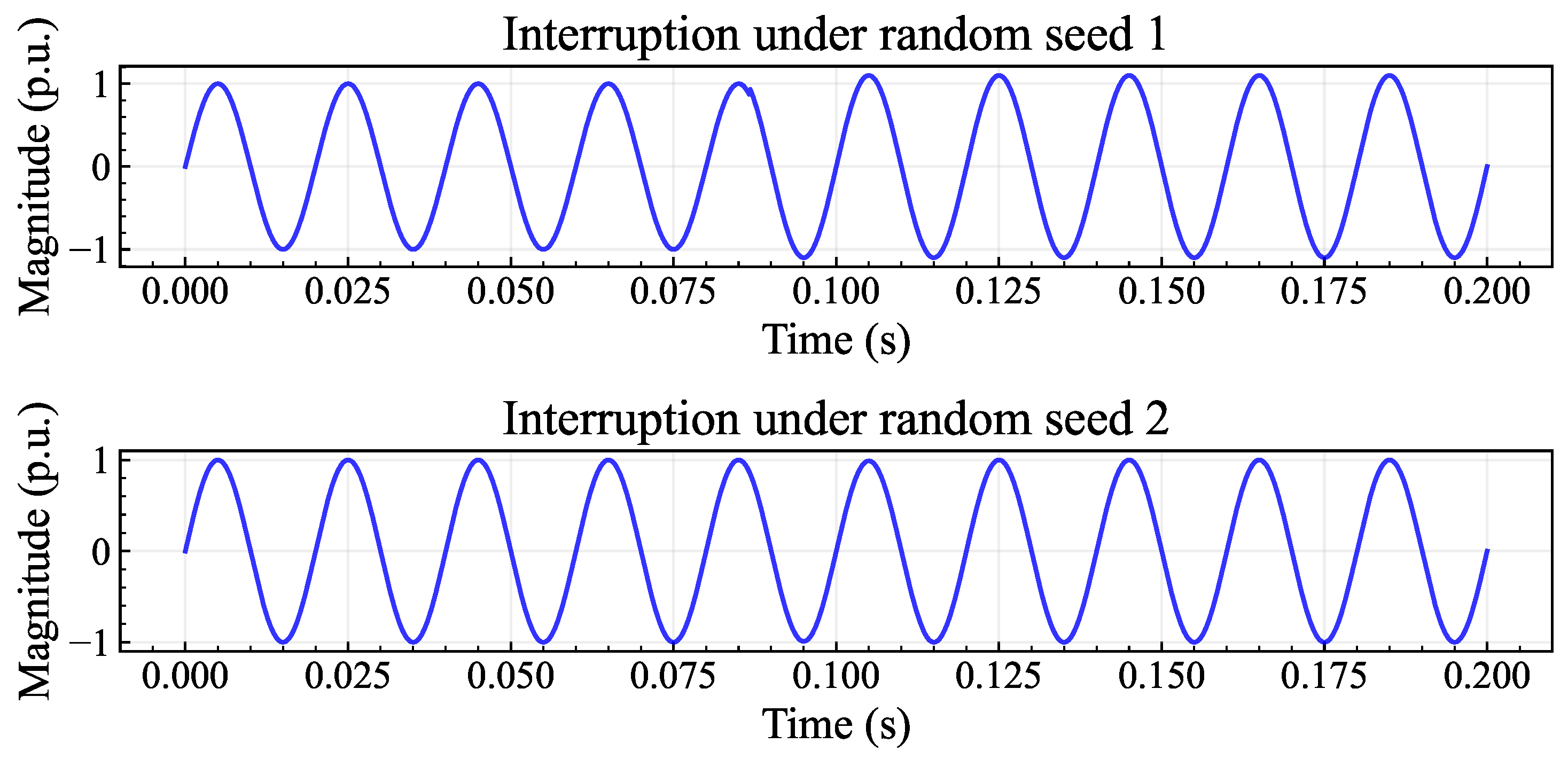
To prevent the same signal segments from being generated, random number and random seed are two key mechanisms. Therein, the random number is applied into the stochastic parameterization of the equations, such as random magnitude scaling parameters, random frequency scaling parameters, random time duration parameters, etc. And a random seed is utilized to ensure that the random parameters output a different value each time. Taking interruption as an example, with n u m p y . r a n d o m . r a n d as r a n d [37], α can be expressed as 0.1 · r a n d ( ) + 0.9 . So under different random seeds, random parameters α , t 1 , t 2 output different values, and the corresponding waveforms of Interruption are shown in Figure 3. Similarly, the waveforms of normal signals are displayed in Figure 4. It can observed that the signal fragments are different under different seeds, thereby ensuring that each simulated signal represents a distinct realization of a disturbance class, thereby producing a diverse and challenging dataset for model validation.
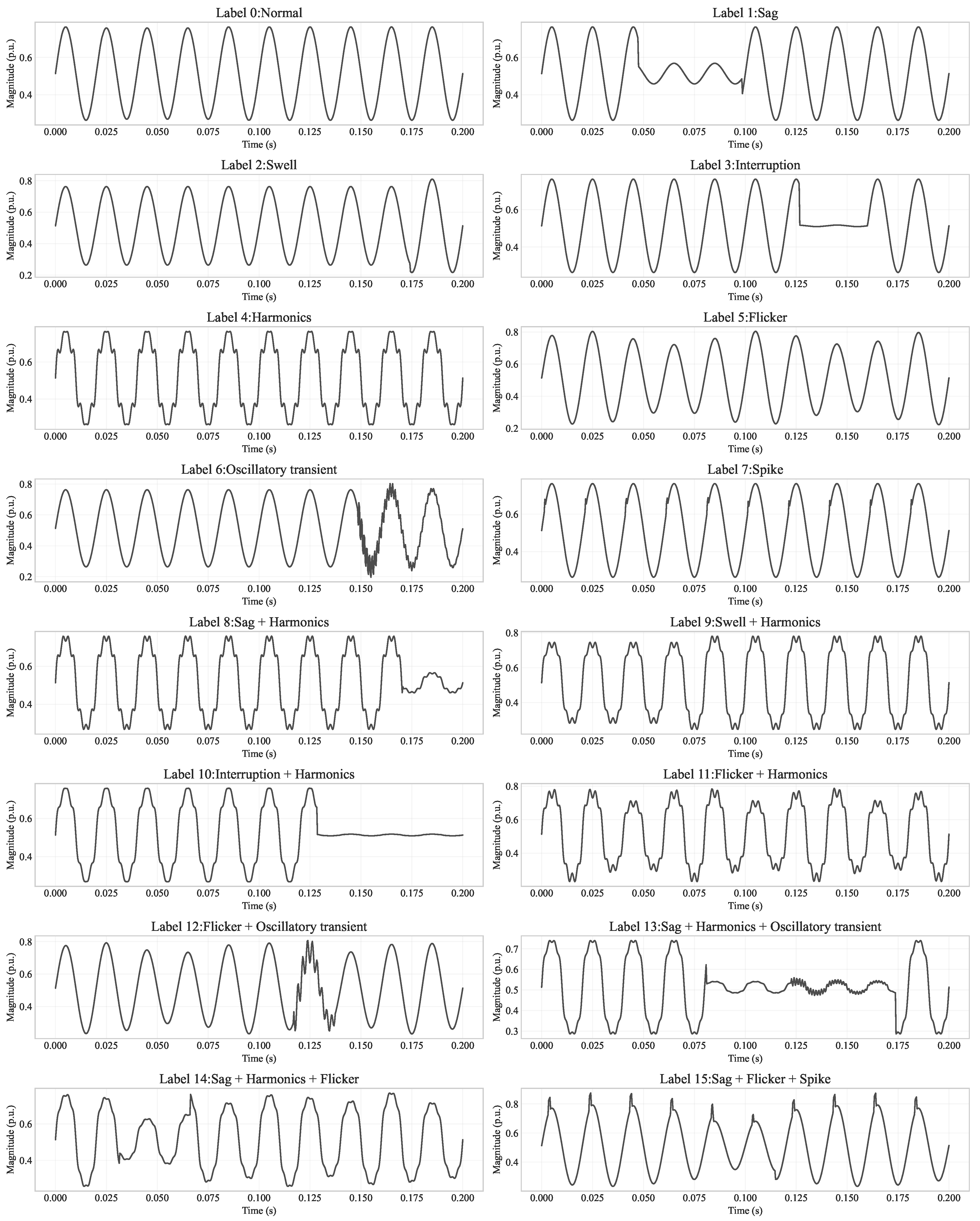
The generated 16 types of signals are visualized in Figure 5. The fundamental frequency f is 50 Hz, and each sample has 10 cycles, so each signal segment length is 0.2 s. The sampling frequency here is set to 3200 Hz, and this means that each sample has 640 sampling points.
Subsequently, the MCAR mechanism is applied to the complete disturbance data to generate a dataset with missing values. To comprehensively evaluate imputation performance, the missing percentage ranges from 10% to 80%.

4.1.2. Experimental Configuration

All experiments were implemented in a Python 3.8.6 [38] environment using Jupyter Notebooks, with the deep learning components built upon the TensorFlow framework. All figures presented in this paper are generated using the Matplotlib 3.5.3 library [39]. The generated dataset comprises a total of 6000 samples, consisting of 1500 samples for normal signals and 300 samples for each disturbance type.
As to the proposed GAI method, the model is trained for a total of 12,000 epochs to guarantee good convergence. During training, the batch size is set to 160. Notably, the random vector Z is drawn from a uniform distribution U ( 0 ,   0.01 ) . For optimization of D and G , Adam optimizers are configured with a conservative learning rate: η = 1 × 10 4 . For the loss of G , the tuning factor γ is set to 1000 according to [11]. Through conducting a sensitivity analysis on the model’s training with different γ values, a γ of 1000 provides the best trade-off. For the loss of D , the optimal clipping factor δ is identified as 0.01 through a systematic greedy search over a set of candidate values. This value is also recommended in [22].
Concerning performance evaluation metrics, both quantitative metrics and qualitative visualization are involved. Quantitative metrics include the root mean squared error (RMSE), mean absolute error (MAE), mean absolute percentage error (MAPE), and coefficient of determination (R2). As a separate note, if R2 reaches 1.0, this implies a superior model fit. For qualitative evaluation, t-distributed stochastic neighbor embedding (t-SNE) is utilized for recovery comparisons.
To validate the efficacy of the proposed GAI, five representative imputation methods are chosen as the benchmarks, including two baselines and three state-of-the-art (SOTA) algorithms. The baselines, mean and forward fill imputation, are not detailed here. And the three SOTA algorithms are listed below:
1.
RF refers to random forest imputation. RF iteratively fits a forest of decision trees to the observed data; then, the model is utilized to predict missing data [19].
2.
SolarGAN performs temporal data imputation by a simple Wasserstein GAN with a weak 1-Lipschitz constraint [23]. The configuration is taken from [11].
3.
EGAIN [20] stands for the enhanced GAIN algorithm. It is enhanced by a structured five-layer MLP with 2560, 640, 640, 640, and 640 units.
For consistency across all experiments, the critical hyperparameters of SOTA methods are kept in alignment with the proposed GAI.

4.2. Imputation Performance Evaluation

The imputation performance evaluation in this section is composed of imputation scoring and characteristic analyses.

4.2.1. Analysis of Imputation Scores

Here, we present a comprehensive analysis of imputation scoring performances. The performance comparison of different imputation methods across different missing rates is demonstrated in Table 2. Generally speaking, the performance of all imputation methods degrades as the missing percentage increases. Notably, the proposed GAI undoubtedly shows superiority across all evaluation metrics and all missing percentages. More specifically, GAI achieves the lowest MAE, MAPE, and RMSE values, indicating the lowest number of imputation errors. At a low missing percentage of 10%, the MAE of the proposed GAI is 28.6% lower than the second-best EGAIN and 54.5% lower than the common RF. When compared to EGAIN under the extreme 80% missingness, the proposed GAI achieves a remarkable decrease of 63.1% in MAE, 61.5% in MAPE, and 73.2% in RMSE. Across all missing percentages, GAI achieves an average MAE reduction of 29.71% in contrast to EGAIN. As for R2, the proposed GAI exhibits very graceful degradation, beginning at a near-perfect R2 of 0.9949 at 10% missingness and maintaining an excellent 0.9336 even when the missing percentage is 80%. In conclusion, these imputation results vigorously validate the superiority of the proposed GAI method, making it practical for challenging real-world applications.
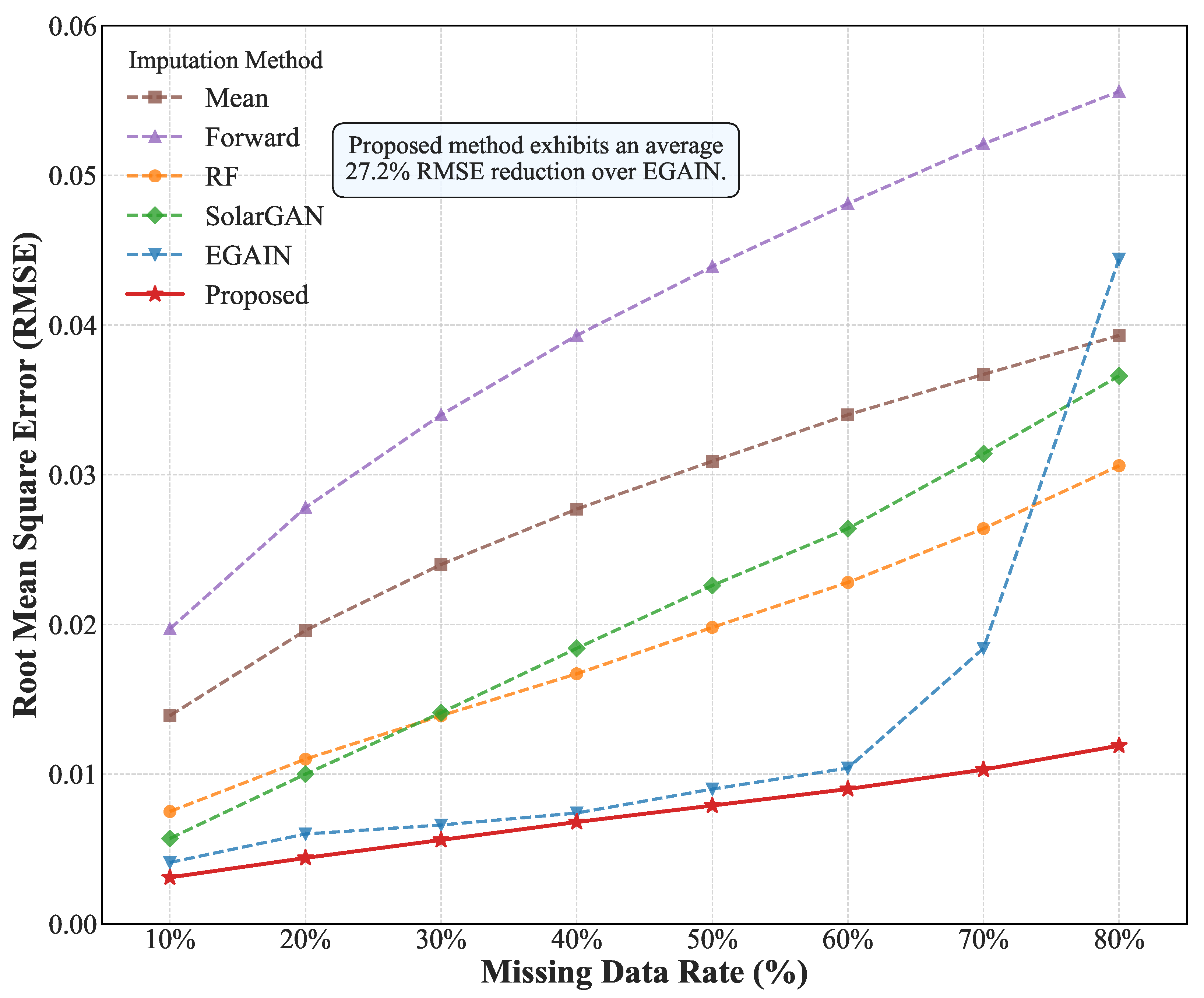
For convenience, the curves of RMSE performance under different missing percentages are displayed in Figure 6. It can be observed that the proposed GAI consistently maintains the lowest RMSE values throughout all missing data percentages. While the runner-up model, EGAIN, maintains stable imputation performance for missingness percentages between 10% and 60%, its performance collapses sharply at missingness levels above 70%, performing worse than the simple forward baseline at 80% missingness. By contrast, the proposed method exhibits an average 27.2% RMSE reduction over EGAIN. Generally, Figure 6 clearly demonstrates the imputation robustness of the proposed GAI across various missingness percentages.
Furthermore, a specific imputation analysis is carried out for each disturbance type. When the missing percentage is 20%, the corresponding performance is displayed in Figure 7. On the whole, it is seen that the proposed GAI achieves a significant MAE reduction for the majority of disturbance types compared to EGAIN. The only exceptions were for flicker + oscillatory transient and interruption disturbances, where the MAE increased by 16.8% and 1.8%, respectively. The underperformance on flicker + oscillatory transient may be attributed to the gating mechanism in the GAI. This mechanism appears to prioritize high-frequency and sharp oscillatory transient features over the lower-frequency characteristics of flicker.
Above all, a rigorous evaluation of imputation scores reveals that the proposed GAI method exhibits exceptional error reduction and robustness, establishing its state-of-the-art performance in this domain.

4.2.2. Analysis of Imputation Characteristics

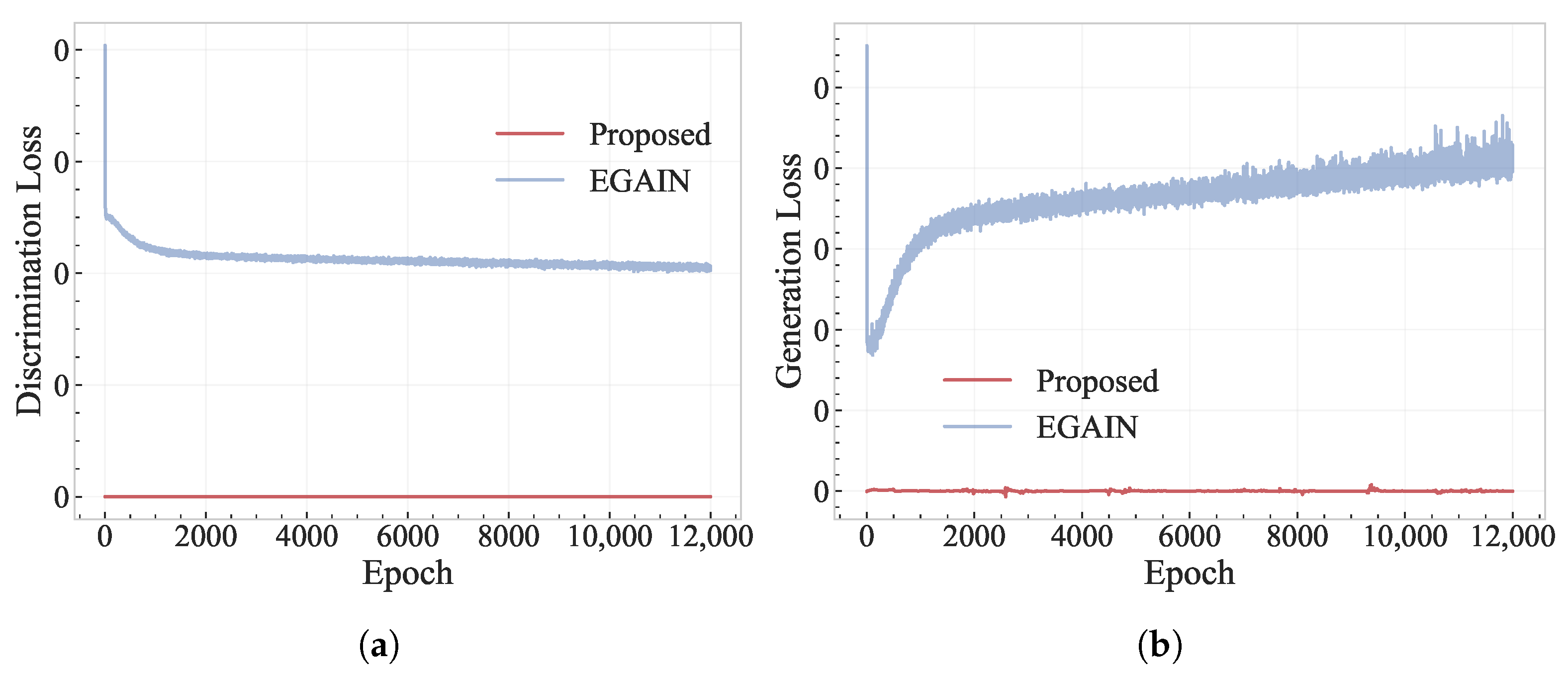
This section describes the analysis of imputation characteristics, comprising the training process, recovery characteristics, and feature representations. Initially, to display the training process, the loss curves at a missingness of 20% are presented in Figure 8. Intuitively, it is observed that the proposed GAI achieves a significantly smoother loss trajectory and converges more instantly and precisely to zero compared to EGAIN. Conversely, the training process of EGAIN is characterized by instability. Therein, the discriminator loss of EGAIN exhibits a terrible convergence, plateauing at a value of approximately 0.4, and its generation loss exhibits continued and high-amplitude oscillations. The results above confirm that the proposed GAI has extraordinary training stability and learning efficiency, benefiting directly from the incorporation of the well-constrained Wasserstein imputation loss.
To visually evaluate the fidelity of the recovered disturbance data, Figure 9 displays the waveforms of the incomplete and recovered signals in the 20% data missingness condition. Together with Figure 5, it is seen that the proposed GAI accurately reconstructs all disturbance types from the missing data. More importantly, the fundamental characteristics and critical features are both preserved with high fidelity. Ultimately, these results highlight the effectiveness of the proposed GAI for high-fidelity signal recovery.
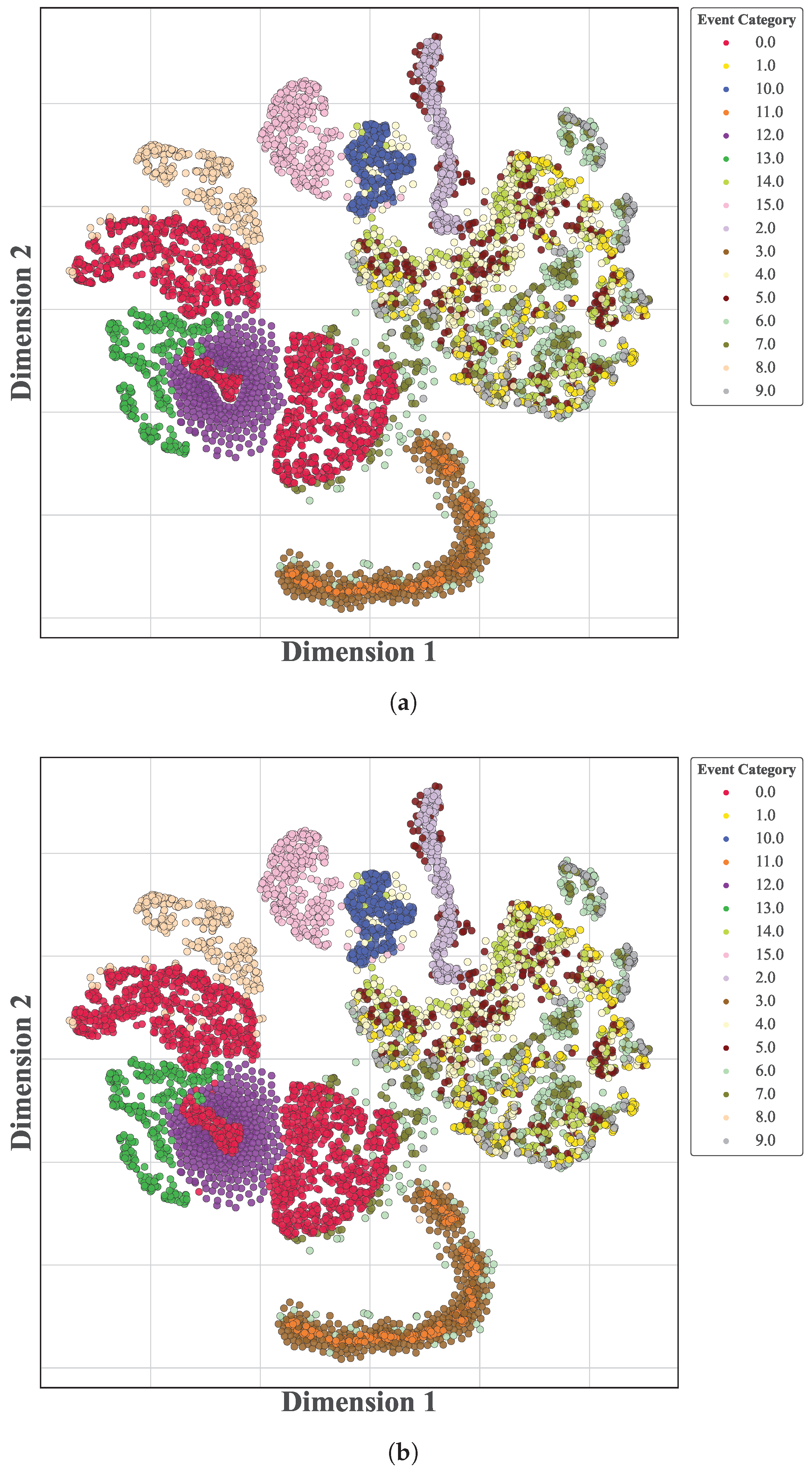
Finally, t-SNE visualization plots are utilized to assess the quality of the feature representation from recovered disturbance data. As demonstrated in Figure 10, the t-SNE analysis reveals that the recovered data forms closed and well-separated clusters for each disturbance type, verifying that essential discriminative information is preserved. Furthermore, the recovered t-SNE is highly similar to the ground-truth one, underscoring the high-fidelity recovery of the original characteristics and crucial features of each disturbance type. Together, these results confirm that the proposed GAI maintains the high-fidelity feature representation of the original disturbance data, ensuring that critical information is preserved across the imputation process.

5. Conclusions

In this paper, an innovative and effective gating adversarial imputation (GAI) framework is proposed for the high-fidelity restoration of missing electrical disturbance data. By uniquely integrating a gating MLP structure with a stable Wasserstein adversarial imputation process, the proposed GAI model achieves both robust feature representation and high imputation accuracy.
To simulate real-world situations, a high-quality dataset comprising 15 distinct disturbance types is generated based on well-defined mathematical parametric equations and subsequently subjected to a widely used missing data mechanism. A comprehensive experimental evaluation validates the exceptional imputation performance of the proposed GAI. In contrast to five representative imputation benchmarks, GAI consistently demonstrates state-of-the-art performances across all tested missing percentages. Notably, it achieved an average RMSE reduction of 27.2% over the runner-up model EGAIN. Beyond its quantitative accuracy, the GAI model exhibits exceptional training stability and rapid convergence, a direct result of its well-constrained Wasserstein loss function. Crucially, the analysis confirmed that GAI preserves the fundamental characteristics and critical features of the original signals, ensuring that essential diagnostic information is precisely recovered. These findings establish GAI as a robust and highly effective solution for high-fidelity data restoration, making it a valuable tool for enhancing the reliability of cyber-physical power system monitoring and analysis. To enhance its robustness and practical utility, future studies will investigate the performance of this imputation framework in scenarios with highly skewed disturbance distributions, which more closely emulate real-world operational data.

Author Contributions

Conceptualization, G.F. and L.C.; methodology, G.F.; software, G.F.; validation, G.F.; formal analysis, G.F. and L.C.; investigation, L.C. and L.W.; resources, L.C. and G.F.; data curation, L.C.; writing—original draft preparation, G.F.; writing—review and editing, L.C. and G.F.; visualization, G.F.; supervision, L.C.; project administration, L.W.; funding acquisition, L.C. and L.W. All authors have read and agreed to the published version of the manuscript.

Funding

This research was funded by the National Natural Science Foundation of China under Grant 62001169 and the Open Foundation of Guangdong Provincial Key Laboratory of Green Energy Technology under Grant KFJJ5.

Institutional Review Board Statement

Not applicable.

Informed Consent Statement

Not applicable.

Data Availability Statement

The original contributions presented in this study are included in this article. Data is contained within the article through simulation generation.

Conflicts of Interest

The authors declare no conflicts of interest.

Abbreviations

The following abbreviations are used in this manuscript:
GAIGating adversarial imputation;
CPPSCyber-physical power system;
MLPMulti-layer perceptron;
PMUPhasor measurement unit;
PQDPower quality disturbance;
MARMissing at random;
MCARMissing completely at random;
MNARMissing not at random;
SOTAState of the art;
EGAINEnhanced generative adversarial imputation net;
RMSERoot mean squared error;
MAEMean absolute error;
MAPEMean absolute percentage error.

References

  1. Feng, G.; Lao, K.W.; Chen, G. Out-of-Distribution Detection of Unknown False Data Injection Attack with Logit-Normalized Bayesian ResNet. IEEE Trans. Smart Grid 2024, 15, 6005–6017. [Google Scholar] [CrossRef]
  2. Sugunaraj, N.; Balaji, S.R.A.; Chandar, B.S.; Rajagopalan, P.; Kose, U.; Loper, D.C.; Mahfuz, T.; Chakraborty, P.; Ahmad, S.; Kim, T.; et al. Distributed Energy Resource Management System (DERMS) Cybersecurity Scenarios, Trends, and Potential Technologies: A Review. IEEE Commun. Surv. Tutor. 2025. [Google Scholar] [CrossRef]
  3. Alvarez-Alvarado, M.S.; Apolo-Tinoco, C.; Ramirez-Prado, M.J.; Alban-Chacón, F.E.; Pico, N.; Aviles-Cedeno, J.; Recalde, A.A.; Moncayo-Rea, F.; Velasquez, W.; Rengifo, J. Cyber-physical power systems: A comprehensive review about technologies drivers, standards, and future perspectives. Comput. Electr. Eng. 2024, 116, 109149. [Google Scholar] [CrossRef]
  4. Vahidi, S.; Ghafouri, M.; Au, M.; Kassouf, M.; Mohammadi, A.; Debbabi, M. Security of wide-area monitoring, protection, and control (WAMPAC) systems of the smart grid: A survey on challenges and opportunities. IEEE Commun. Surv. Tutor. 2023, 25, 1294–1335. [Google Scholar] [CrossRef]
  5. Theodorakatos, N.P.; Babu, R. Hybrid Optimization Strategies for Global Optimality in Non-Convex Programming Using SQP and IPMs: Avoiding the Maratos Effect in PMU Placement–A Case Study. J. Phys. Conf. Ser. 2025, 3027, 012041. [Google Scholar] [CrossRef]
  6. Phadke, A.G.; Bi, T. Phasor measurement units, WAMS, and their applications in protection and control of power systems. J. Mod. Power Syst. Clean Energy 2018, 6, 619–629. [Google Scholar] [CrossRef]
  7. Theodorakatos, N.P.; Babu, R.; Theodoridis, C.A.; Moschoudis, A.P. Mathematical models for the single-channel and multi-channel PMU allocation problem and their solution algorithms. Algorithms 2024, 17, 191. [Google Scholar] [CrossRef]
  8. Tang, H.; Wu, J.; Chen, L.; Liu, Z.; Wu, F.; Li, K.; Wu, Z.; Yu, F.; Bi, Q. A control optimization model for CVaR risk of distribution systems with PVs/DSs/EVs using Q-learning powered adaptive differential evolution algorithm. Int. J. Electr. Power Energy Syst. 2021, 132, 107209. [Google Scholar]
  9. Xygkis, T.C.; Löfberg, J.; Korres, G.N. Investigation of Optimal Phasor Measurement Selection for Distribution System State Estimation Under Various Uncertainties. IEEE Trans. Instrum. Meas. 2025, 74, 1–16. [Google Scholar] [CrossRef]
  10. Ravi, T.; Sathish Kumar, K. Analysis, monitoring, and mitigation of power quality disturbances in a distributed generation system. Front. Energy Res. 2022, 10, 989474. [Google Scholar] [CrossRef]
  11. Feng, G.; Lao, K.W. Wasserstein Adversarial Learning for Identification of Power Quality Disturbances with Incomplete Data. IEEE Trans. Ind. Inform. 2023, 19, 10401–10411. [Google Scholar] [CrossRef]
  12. Du, J.; Hu, M.; Zhang, W. Missing data problem in the monitoring system: A review. IEEE Sensors J. 2020, 20, 13984–13998. [Google Scholar] [CrossRef]
  13. Elimam, M.; Isbeih, Y.J.; Azman, S.K.; El Moursi, M.S.; Al Hosani, K. Deep learning-based PMU cyber security scheme against data manipulation attacks with WADC application. IEEE Trans. Power Syst. 2022, 38, 2148–2161. [Google Scholar] [CrossRef]
  14. Li, Z.; Liu, H.; Zhao, J.; Bi, T.; Yang, Q. A power system disturbance classification method robust to PMU data quality issues. IEEE Trans. Ind. Inform. 2021, 18, 130–142. [Google Scholar] [CrossRef]
  15. Zhu, L.; Lin, J. Learning spatiotemporal correlations for missing noisy PMU data correction in smart grid. IEEE Internet Things J. 2020, 8, 7589–7599. [Google Scholar] [CrossRef]
  16. Wang, Y.; Hespanha, J.P. Distributed estimation of power system oscillation modes under attacks on GPS clocks. IEEE Trans. Instrum. Meas. 2018, 67, 1626–1637. [Google Scholar] [CrossRef]
  17. Foggo, B.; Yu, N. Online PMU Missing Value Replacement Via Event-Participation Decomposition. IEEE Trans. Power Syst. 2021, 37, 488–496. [Google Scholar] [CrossRef]
  18. Ribeiro, S.M.; Castro, C. Missing data in time series: A review of imputation methods and case study. Learn. Nonlinear Model. 2022, 20, 31–46. [Google Scholar] [CrossRef]
  19. Hong, S.; Lynn, H.S. Accuracy of random-forest-based imputation of missing data in the presence of non-normality, non-linearity, and interaction. BMC Med Res. Methodol. 2020, 20, 199. [Google Scholar] [CrossRef]
  20. Yoon, J.; Jordon, J.; Schaar, M. Gain: Missing data imputation using generative adversarial nets. In Proceedings of the International Conference on Machine Learning, Stockholm, Sweden, 10–15 July 2018; pp. 5689–5698. [Google Scholar]
  21. Li, Q.; Yang, X.; Xie, X.; Liu, G. The data recovery strategy on machine learning against false data injection attacks in power cyber physical systems. Meas. Control 2025, 58, 632–642. [Google Scholar] [CrossRef]
  22. Arjovsky, M.; Chintala, S.; Bottou, L. Wasserstein generative adversarial networks. In Proceedings of the International Conference on Machine Learning, Sydney, Australia, 6–11 August 2017; pp. 214–223. [Google Scholar]
  23. Zhang, W.; Luo, Y.; Zhang, Y.; Srinivasan, D. SolarGAN: Multivariate Solar Data Imputation Using Generative Adversarial Network. IEEE Trans. Sustain. Energy 2021, 12, 743–746. [Google Scholar] [CrossRef]
  24. Liu, H.; Dai, Z.; So, D.; Le, Q.V. Pay attention to mlps. Adv. Neural Inf. Process. Syst. 2021, 34, 9204–9215. [Google Scholar]
  25. Caicedo, J.E.; Agudelo-Martínez, D.; Rivas-Trujillo, E.; Meyer, J. A systematic review of real-time detection and classification of power quality disturbances. Prot. Control Mod. Power Syst. 2023, 8, 1–37. [Google Scholar] [CrossRef]
  26. Martinez, R.; Castro, P.; Arroyo, A.; Manana, M.; Galan, N.; Moreno, F.S.; Bustamante, S.; Laso, A. Techniques to locate the origin of power quality disturbances in a power system: A review. Sustainability 2022, 14, 7428. [Google Scholar] [CrossRef]
  27. Razo-Hernandez, J.R.; Valtierra-Rodriguez, M.; Amezquita-Sanchez, J.P.; Granados-Lieberman, D.; Gomez-Aguilar, J.F.; Rangel-Magdaleno, J.d.J. Homogeneity-PMU-based method for detection and classification of power quality disturbances. Electronics 2018, 7, 433. [Google Scholar] [CrossRef]
  28. Chen, S.; Li, Z.; Pan, G.; Xu, F. Power quality disturbance recognition using empirical wavelet transform and feature selection. Electronics 2022, 11, 174. [Google Scholar] [CrossRef]
  29. IEEE Std 1159-2019; IEEE Recommended Practice for Monitoring Electric Power Quality. IEEE: Piscataway, NJ, USA, 2019. [CrossRef]
  30. Little, R.J. Missing data assumptions. Annu. Rev. Stat. Its Appl. 2021, 8, 89–107. [Google Scholar] [CrossRef]
  31. Heitjan, D.F.; Basu, S. Distinguishing “missing at random” and “missing completely at random”. Am. Stat. 1996, 50, 207–213. [Google Scholar] [PubMed]
  32. Moreno-Betancur, M.; Chavance, M. Sensitivity analysis of incomplete longitudinal data departing from the missing at random assumption: Methodology and application in a clinical trial with drop-outs. Stat. Methods Med. Res. 2016, 25, 1471–1489. [Google Scholar] [CrossRef] [PubMed]
  33. Jamshidian, M.; Jalal, S. Tests of homoscedasticity, normality, and missing completely at random for incomplete multivariate data. Psychometrika 2010, 75, 649–674. [Google Scholar] [CrossRef] [PubMed]
  34. Steck, H. Training and testing of recommender systems on data missing not at random. In Proceedings of the 16th ACM SIGKDD International Conference on Knowledge Discovery and Data Mining, Washington, DC, USA, 25–28 June 2010; pp. 713–722. [Google Scholar]
  35. Li, Q.; Xu, Y.; Chew, B.S.H.; Ding, H.; Zhao, G. An integrated missing-data tolerant model for probabilistic PV power generation forecasting. IEEE Trans. Power Syst. 2022, 37, 4447–4459. [Google Scholar] [CrossRef]
  36. Petzka, H.; Fischer, A.; Lukovnikov, D. On the regularization of Wasserstein GANs. In Proceedings of the International Conference on Learning Representations, Vancouver, BC, Canada, 30 April–3 May 2018. [Google Scholar]
  37. Harris, C.R.; Millman, K.J.; Van Der Walt, S.J.; Gommers, R.; Virtanen, P.; Cournapeau, D.; Wieser, E.; Taylor, J.; Berg, S.; Smith, N.J.; et al. Array programming with NumPy. Nature 2020, 585, 357–362. [Google Scholar] [CrossRef] [PubMed]
  38. Van Rossum, G.; Drake, F.L., Jr. Python Tutorial; Centrum voor Wiskunde en Informatica: Amsterdam, The Netherlands, 1995; Volume 620. [Google Scholar]
  39. Hunter, J.D. Matplotlib: A 2D graphics environment. Comput. Sci. Eng. 2007, 9, 90–95. [Google Scholar] [CrossRef]
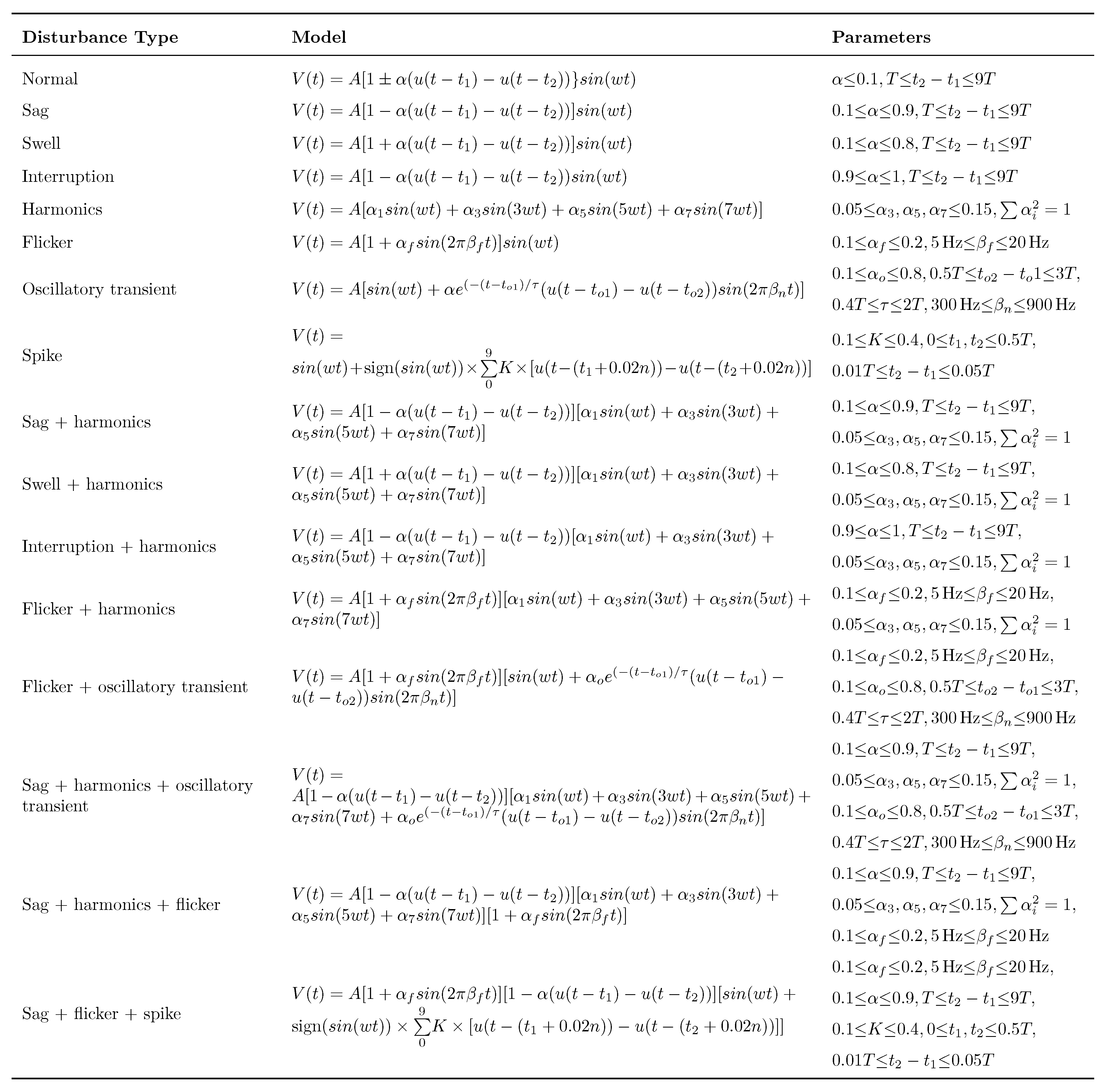
Figure 1. Mathematical modeling of electrical disturbance signals.
Electronics 14 04108 g001
Figure 2. Flowchart of the proposed gating adversarial imputation (GAI).
Electronics 14 04108 g002
Figure 3. Waveforms of interruption under different random seeds.
Electronics 14 04108 g003
Figure 4. Waveforms of normal voltage signals under different random seeds.
Electronics 14 04108 g004
Figure 5. Waveforms of 16 electrical disturbance types.
Electronics 14 04108 g005
Figure 6. RMSE curves of various imputation methods across different missing percentages.
Electronics 14 04108 g006
Figure 7. MAE performance for each disturbance type under a missing percentage of 20%.
Electronics 14 04108 g007
Figure 8. Training loss curves of EGAIN and the proposed GAI: (a) discrimination loss. (b) generation loss.
Electronics 14 04108 g008
Figure 9. Waveforms of incomplete and recovered disturbance data.
Electronics 14 04108 g009
Figure 10. t-SNE plots of ground-truth and recovered disturbance data: (a) ground-truth disturbance data; (b) recovered disturbance data.
Electronics 14 04108 g010
Table 1. Disturbance types and their corresponding labels.
LabelDisturbance TypeLabelDisturbance Type
0Normal8Sag + harmonics
1Sag9Swell + harmonics
2Swell10Interruption + harmonics
3Interruption11Flicker + harmonics
4Harmonics12Flicker + oscillatory transient
5Flicker13Sag + harmonics + oscillatory transient
6Oscillatory transient14Sag + harmonics + flicker
7Spike15Sag + flicker + spike
Table 2. Performance comparison of imputation methods across different missing rates.
Missing
Percentage
MeanForwardRFSolarGANEGAINProposed
MAE (Mean Absolute Error)
10%0.00290.00410.00110.00100.00070.0005
20%0.00580.00810.00230.00270.00140.0009
30%0.00870.01220.00370.00480.00190.0014
40%0.01160.01630.00540.00710.00240.0021
50%0.01450.02030.00750.00990.00340.0027
60%0.01740.02440.00970.01280.00430.0034
70%0.02030.02850.01280.01620.00600.0042
80%0.02320.03250.01630.02000.01490.0055
MAPE (Mean Absolute Percentage Error)
10%0.00670.00930.00240.00230.00160.0010
20%0.01330.01850.00530.00600.00330.0021
30%0.01990.02780.00860.01080.00420.0032
40%0.02660.03720.01240.01620.00550.0046
50%0.03320.04630.01720.02240.00770.0060
60%0.03990.05570.02240.02940.00990.0076
70%0.04660.06510.02930.03710.01290.0095
80%0.05310.07430.03750.04570.03170.0122
RMSE (Root Mean Square Error)
10%0.01390.01970.00750.00570.00410.0031
20%0.01960.02780.01100.01000.00600.0044
30%0.02400.03400.01390.01410.00660.0056
40%0.02770.03930.01670.01840.00740.0068
50%0.03090.04390.01980.02260.00900.0079
60%0.03400.04810.02280.02640.01040.0090
70%0.03670.05210.02640.03140.01840.0103
80%0.03930.05560.03060.03660.04440.0119
R2 (Coefficient of Determination)
10%0.89940.79800.96490.96970.99320.9949
20%0.79940.59820.92690.88300.98790.9907
30%0.70010.39770.88260.84160.97970.9855
40%0.59900.19650.83400.76280.97450.9784
50%0.5000−0.00390.77060.64740.96320.9706
60%0.3997−0.19930.70110.47970.95050.9618
70%0.3009−0.40160.60600.32380.84560.9495
80%0.2002−0.59920.47310.13560.10770.9336
Disclaimer/Publisher’s Note: The statements, opinions and data contained in all publications are solely those of the individual author(s) and contributor(s) and not of MDPI and/or the editor(s). MDPI and/or the editor(s) disclaim responsibility for any injury to people or property resulting from any ideas, methods, instructions or products referred to in the content.