Finite-Time Fuzzy Tracking Control for Two-Stage Continuous Stirred Tank Reactor: A Gradient Descent Approach via Armijo Line Search

Abstract

This paper proposes a novel finite-time adaptive fuzzy control strategy for two-stage continuous stirred tank reactor (CSTR) systems. The method integrates the gradient descent (GD) algorithm with Armijo line search to dynamically adjust the learning rate, thereby optimizing the parameters of fuzzy logic systems (FLSs) for fast and accurate approximation of unknown nonlinear functions. The proposed control scheme, based on finite-time stability theory, ensures convergence of system states to the desired trajectory within finite time. Compared with conventional adaptive fuzzy control methods, the approach effectively addresses the issues of slow convergence and low approximation accuracy, significantly reducing approximation error while enhancing convergence performance. Simulation results on a two-stage CSTR system verify that the proposed controller achieves rapid convergence and high approximation accuracy.

1. Introduction

Continuous stirred tank reactor (CSTR) systems serve as core equipment in industrial processes such as petrochemicals, bio-pharmaceuticals, and chemical manufacturing [1,2]. The continuous mixing and agitation in CSTR systems ensure reaction stability and uniformity. Accurate control of variables, including temperature, pressure, and material flow rate, enables the regulation of reaction kinetics and product outcomes, thereby improving process accuracy. This is particularly critical in processes requiring high-purity products, where even minor deviations can lead to significant yield losses. In recent years, with advances in industrial production, interconnected multi-reactor configurations have become increasingly common, and two-stage CSTR systems are widely used in chemical production. These systems not only improve the overall reactant conversion rate but also reduce total reaction costs. However, controlling CSTR systems remains challenging due to their complex nonlinear dynamics, time-varying characteristics, and strong mass–heat transfer coupling.

During the early period of industrial applications, Proportional–Integral–Derivative (PID) control algorithms [3,4] were widely applied in CSTR systems due to their simple structure and ease of implementation. However, as the demand for high precision, fast dynamic response, and strong anti-interference capabilities in chemical processes increases, traditional PID control methods struggle to meet these requirements. In recent years, research on CSTR control has gradually shifted to nonlinear methods, such as sliding mode control (SMC) [5,6,7], model predictive control (MPC) [8,9], and feedback linearization [10,11]. For two-stage CSTR systems, Reference [8] proposed an MPC method with parameter-adaptive correction, while Reference [6] introduced a distributed output consensus framework integrating integral SMC and MPC. Additionally, Reference [12] implemented a model reference adaptive control (MRAC) method based on the MIT rule for temperature control of the cascaded CSTR systems.

These methods have shown superior performance in handling nonlinear dynamics, but they often require accurate system models or complex parameter tuning, which limits their practical application. In related works, fuzzy logic systems (FLSs) [13,14,15,16] and neural networks (NNs) [17,18,19] have been extensively applied to approximate unknown nonlinear functions relying on their powerful nonlinear approximation and self-regulation capabilities. In the engineering domain, FLSs have been applied to the activated sludge process in Reference [20], and FLSs have also been leveraged for fault diagnosis and safety protection in Reference [21]. For two-stage CSTR systems, Reference [22] employed a fuzzy logic system (FLS) to approximate unknown functions and developed an adaptive control framework, while Reference [23] proposed a fuzzy adaptive control method for CSTR systems subject to full-state constraints and actuator faults.

Although FLSs can effectively approximate nonlinear functions, their adaptive law parameter update rules are complex, and the design of fuzzy basis functions is often limited by experience, resulting in insufficient approximation accuracy. Therefore, improving the approximation capability of fuzzy systems has gained attention. Reference [24] remodeled the approximation error with traditional fixed constants as a time-varying function and leveraged online fuzzy inference for real-time compensation. Meanwhile, References [25,26] have proposed adaptive NN controllers that optimize parameter updates using a gradient descent (GD) algorithm, which provides an effective approach for parameter adaptive control. However, investigations that apply GD to optimize the parameter-update mechanism in fuzzy control systems remain limited. Furthermore, most existing works rely on the GD algorithm with a fixed step size. Although this method is simple, it struggles to balance iteration efficiency and convergence stability.

Furthermore, most current approaches typically rely on uniform ultimate boundedness theory, which guarantees system convergence only as time approaches infinity. However, practical engineering applications often require the system to reach a stable state within a finite time. For instance, in the chemical batch processes, reaction time directly impacts production efficiency and energy consumption. Consequently, finite-time control (FTC) theory has gradually become a prominent research focus, as demonstrated in [27,28,29,30], which explores FTC applications in various industrial scenarios. Among the most widely adopted techniques are homogeneous FTC, adding power integrator, fractional power state feedback, and terminal sliding mode (TSM) control, which have shown remarkable effectiveness in handling nonlinear system dynamics. On this basis, theoretical breakthroughs form the foundation of engineering applications. References [31,32] first established a Lyapunov-based finite-time stability theory. This theory innovatively introduces fractional-order Lyapunov functions to ensure convergence within a pre-specified time bound, marking a breakthrough from traditional infinite-time stability analysis. Then, according to the Lyapunov method, the finite-time stabilization problem for nonlinear systems has been extensively handled in References [33,34,35,36]. Reference [37] proposed a finite-time adaptive fuzzy control strategy. However, it is only applicable to strict-feedback systems. A novel finite-time adaptive fuzzy control strategy for pure-feedback systems is designed in [38], which overcomes the strict-feedback constraint by integrating an NNs approximation with terminal sliding mode control (TSMC). For CSTR systems, Reference [39] proposed a finite-time adaptive fuzzy control method that employs an integral barrier Lyapunov function (iBLF) to handle output constraints with a finite-time adaptive controller, while Reference [23] focused on adaptive fixed-time fuzzy controllers for CSTR systems. Nevertheless, most studies target single-stage CSTR systems, and finite-time control specifically for two-stage CSTR systems remains limited.

To address the challenges of improving convergence accuracy and speed, this paper proposes a finite-time adaptive fuzzy control system based on the GD algorithm with Armijo line search. The main contributions of this paper are as follows:

• References [34,38] adopt NN-type adaptive controllers that use a constant learning rate for parameter updates. This paper optimizes the FLS parameters by GD algorithm with Armijo line search on a cost tied to the FLS approximation error. The Armijo rule adaptively selects the step size, reducing manual retuning and improving convergence reliability. To the best of our knowledge, this is the first application of GD-based FLSs tuning with Armijo line search to a two-stage CSTR system.
• Reference [26] establishes an asymptotic stability controller rather than finite-time stability. Such a guarantee lacks a deterministic settling-time bound, which is often mandatory for two-stage CSTR systems. In contrast, this paper integrates FLSs with finite-time stability criteria, ensuring that the states reach the desired trajectories within a finite time. Consequently, the proposed method meets fast-response requirements for two-stage CSTR systems.

The rest of this paper is organized as follows. Section 2 first reviews the necessary preliminaries and formulates the problem, and establishes the nonlinear dynamic model of the two-stage CSTR system. In Section 3, we propose an adaptive fuzzy tracking control method for the transformed nonlinear system and carry out the convergence analyses. In Section 4, we analyze computational complexity of the proposed method. Section 5 demonstrates the effectiveness of the proposed method through simulation examples. Finally, Section 6 concludes the paper.

Notation: Throughout this paper, $V_A$ and $V_B$ denote the reactor volumes; $R_A$ and $R_B$ the recirculation rates; $F_A$ and $F_B$ the outlet flows; ${\theta }_A$ and ${\theta }_B$ the reaction time constants; and F the inlet flow that delivers feed concentration $C_F$ to reactor B. $K_A$ and $K_B$ represent temperature-invariant reaction rate constants; $C_A$ and $C_B$ the product concentrations of reactors A and B; $x_1$ and $x_2$ are the system states; u the control input; $y_d$ and ${\dot{y}}_d$ the reference signal and its derivative, respectively; and $e_1$ and $e_2$ the tracking errors; ${\alpha }_1$ denotes the virtual control; E the error energy; J the cost function; V the Lyapunov function; and $\eta$ the step size of the GD algorithm. For adaptive fuzzy approximations, the parameters used are ${\widehat{\theta }}_1$ and ${\widehat{\theta }}_2$, paired with basis functions ${\varphi }_1(·)$, ${\varphi }_2(·)$, while $d_1$ and $d_2$ denote noise. All these notations are used consistently throughout the paper.

2. Preliminaries and Problem Description

2.1. Preliminaries

 Definition 1

([40]). The equilibrium point $x=0$ of the nonlinear system $\dot{x}=f\left(x\right)$ is semi-global practical finite-time stable (SGPFS) if, for every initial condition $x\left(t_0\right)=x_0$, there exists a sufficiently small positive number $\epsilon >0$ and a finite settling time $T(\epsilon ,x_0)<\infty$ such that the state $x\left(t\right)$ satisfies $\parallel x\left(t\right)\parallel <\epsilon ,\forall t\ge t_0+T$.

 Lemma 1

([41]). For $a_i\in \mathbb{R},i=1,\dots ,n,0<p\le 1$, the following relationship holds

$$\begin{array}{c}\hfill (\sum _{i=1}^n|a_i{|)}^p\le \sum _{i=1}^n|a_i{{|}^p\le n^{1-p}(\sum _{i=1}^n|a_i|)}^p.\end{array}$$

(1)

 Lemma 2

([42]). For real variables z and ζ, and any positive constants μ, θ, and ι, the following inequality holds

$$\begin{array}{c}\hfill {\left|z\right|}^{\mu }{\left|\zeta \right|}^{\theta }\le {\displaystyle \frac{\mu }{\mu +\theta }}{\iota \left|z\right|}^{\mu +\theta }+{\displaystyle \frac{\theta }{\mu +\theta }}{\iota }^{-{\displaystyle \frac{\mu }{\theta }}}{\left|\zeta \right|}^{\mu +\theta }.\end{array}$$

(2)

 Lemma 3

([38]). Consider the nonlinear system $\dot{x}=f\left(x\right)$. If there exists a smooth positive-definite function $V\left(x\right)$ and constants $c>0$, $0<\beta <1$, $\varrho >0$, and $0<\zeta <1$ such that

$$\dot{V}\left(x\right)\le -c{V}^{\beta }\left(x\right)+\varrho ,\forall t\ge 0,$$

(3)

then the system is SGPFS. Moreover, the trajectory $x\left(t\right)$ converges to the set

$${\Omega }_x=\left\{x\mid V^{\beta }\left(x\right)\le {\displaystyle \frac{\varrho }{(1-\zeta )c}}\right\}$$

(4)

within a finite time $T_r$ bounded by

$$T_r\le {\displaystyle \frac{1}{(1-\beta )\zeta c}}\left[V^{1-\beta }\left(x\left(0\right)\right)-{\left({\displaystyle \frac{\varrho }{(1-\zeta )c}}\right)}^{(1-\beta )/\beta }\right].$$

(5)

2.2. Two-Stage Continuous Stirred Tank Reactor Systems

This study focuses on a two-stage CSTR system. As shown in Figure 1, the system employs a series-connected dual reactor, which is frequently considered in the chemical industry [43,44]. This modular design enables stage-specific control of operational conditions like residence time and reactant mixing profiles, allowing optimal adaptation to complex reaction kinetics and product quality requirements. The dynamic behavior of the system is governed by its operational and design parameters, which are shown in

Table 1. Symbols and units of the two-stage continuous stirred tank reactor model.

Symbol	Model Variable	Unit
$C_F$	Feed Concentration	$\mathrm{mol}/\mathrm{L}$
$C_A$, $C_B$	Outlet Concentration	$\mathrm{mol}/\mathrm{L}$
$R_A$, $R_B$	Recirculation Flow Rate	$\mathrm{L}/\min$
$K_A$, $K_B$	Reaction Constant	${\min }^{-1}$
F	Feed Flow Rate	$\mathrm{L}/\min$
$F_A$, $F_B$	Outlet Flow Rate	$\mathrm{L}/\min$
$V_A$, $V_B$	Reactor Volume	L
${\theta }_A$, ${\theta }_B$	Reaction Time	min

.

To facilitate analysis, it is assumed that the reaction temperature is maintained at a constant value in both reactors. Fixing the temperature simplifies the model while still capturing the essential interactions between mass transfer and chemical reactions. In this case, the key controlled variables are the product concentrations $C_A$ and $C_B$ from reactors A and B, respectively, along with the feed concentration $C_F$. In particular, $C_A$ and $C_B$ reflect conversion and selectivity across the two stages and determine the downstream composition. Their regulation via $C_F$ and the flow and recirculation settings shapes the system’s transient and steady state behavior. Under ideal conditions, the governing Equation (6) can be derived through material and energy balance principles.

$$\begin{array}{c}\hfill \left\{\begin{array}{c}{V}_A{\dot{C}}_A=(1-R_B)C_B-F_A{C}_A-V_A{K}_A{C}_A\hfill \\ V_B{\dot{C}}_B=F{C}_F+R_A{C}_A-F_B{C}_B-V_B{K}_B{C}_B\hfill \end{array}\right.\end{array}$$

(6)

According to Equation (6), the residence times are defined by ${\displaystyle \frac{1}{{\theta }_A}}={\displaystyle \frac{F_A}{V_A}}$ and ${\displaystyle \frac{1}{{\theta }_B}}={\displaystyle \frac{F_B}{V_B}}$, linking each reactor’s outlet flow rate to its volume. For compactness, define states $x_1=C_A$ and $x_2=C_B$, and the input $u=C_F$. With these definitions, the material balances in Equation (6) can be written in concise form as

$$\begin{array}{c}\hfill \left\{\begin{array}{c}{\dot{x}}_1={\displaystyle \frac{1-R_B}{V_A}}{x}_2-({\displaystyle \frac{1}{{\theta }_A}}+K_A)x_1\hfill \\ {\dot{x}}_2={\displaystyle \frac{F}{V_B}}u+{\displaystyle \frac{R_A}{V_B}}{x}_1-({\displaystyle \frac{1}{{\theta }_B}}+K_B)x_2.\hfill \end{array}\right.\end{array}$$

(7)

Define $k_1={\displaystyle \frac{1-R_B}{V_A}},k_2={\displaystyle \frac{F}{V_B}},f_1\left(x_1\right)=-({\displaystyle \frac{1}{{\theta }_A}}+K_A)x_1$, and $f_2\left({\overline{x}}_2\right)={\displaystyle \frac{R_A}{V_B}}{x}_1-({\displaystyle \frac{1}{{\theta }_B}}+K_B)x_2$, where ${\overline{x}}_2$ denotes the state vector ${[x_1,x_2]}^T$. Thus, the system (7) can be concisely expressed as

$$\left\{\begin{array}{c}{\dot{x}}_1=k_1{x}_2+f_1\left(x_1\right)\hfill \\ {\dot{x}}_2=k_{2}u+f_2\left({\overline{x}}_2\right)\hfill \\ y=x_1\hfill \end{array}\right.$$

(8)

where $x_1,x_2\in \mathbb{R}$, $u\in \mathbb{R}$, and $y\in \mathbb{R}$ denote the system states, control input, and output, respectively. The functions $f_i(·)$ for $i=1,2$ are unknown, while $k_1$ and $k_2$ are known constants. The objective of this paper is to design a control input u such that the output y accurately tracks a given reference signal $y_d$, with all signals remaining bounded. Define a vector function ${\overline{y}}_d={[y_d,{\dot{y}}_d]}^T$, where ${\dot{y}}_d$ denotes the first-order derivative of $y_d$. To facilitate controller design, the following assumptions are introduced.

 Assumption 1.

The desired trajectory $y_d\left(t\right)$ and its first-order derivative ${\dot{y}}_d$ are continuous and known, with both being uniformly bounded.

 Assumption 2.

The unknown functions $f_i(·)$ for $i=1,2$ are smooth and continuous.

 Remark 1.

The smoothness and continuity of the unknown functions $f_i(·)$ in Assumption 2 guarantee that system dynamics are free of discontinuities or singularities, enabling Lyapunov-based stability analysis.

2.3. Fuzzy Logic Systems

In this paper, a fuzzy logic system is employed to approximate the unknown nonlinear functions $f_i(·)$ for $i=1,2$. The set of IF-THEN rules can be expressed as

$$\begin{array}{cc}\hfill R_i:& \mathrm{IF}{x}_1\mathrm{is}{F}_1^i,\mathrm{and}\cdots \mathrm{and},x_n\mathrm{is}{F}_n^i,\hfill \\ & \mathrm{THEN}y\mathrm{is}{B}^i,i=1,2,\dots ,N\hfill \end{array}$$

where $x=[x_1,\dots ,x_n]\in {\mathbb{R}}^n$ represents the input variable, $y\in \mathbb{R}$ is the output variable, and $F_j^i,B^i,j=1,2,\dots ,n$ are fuzzy sets, N denotes the total number of fuzzy rules.

By using the singleton fuzzifier, product inference, and center-average defuzzifier, the fuzzy logic system can be expressed as

$$\begin{array}{c}\hfill y\left(x\right)={\displaystyle \frac{{\sum }_{i=1}^N{\Theta }_i{\prod }_{j=1}^n{\mu }_{F_j^i}\left(x_j\right)}{{\sum }_{i=1}^N\left[{\prod }_{j=1}^n{\mu }_{F_j^i}\left(x_j\right)\right]}}\end{array}$$

(9)

where ${\mu }_{F_j^i}\left(x_j\right)$ is the membership function of $F_j^i$, and ${\Theta }_i=ma{x}_{y\in R}{\mu }_{B^i}\left(y\right)$. Define $\theta ={[{\Theta }_1,{\Theta }_2,\dots ,{\Theta }_N]}^T$, and the fuzzy basis function ${\varphi }_i\left(x\right)$ is expressed as

$$\begin{array}{c}\hfill {\varphi }_i\left(x\right)={\displaystyle \frac{{\prod }_{j=1}^n{\mu }_{F_j^i}\left(x_j\right)}{{\sum }_{i=1}^N\left[{\prod }_{j=1}^n{\mu }_{F_j^i}\left(x_j\right)\right]}}.\end{array}$$

(10)

Define $\varphi \left(x\right)={[{\varphi }_1\left(x\right),{\varphi }_2\left(x\right),\dots ,{\varphi }_N\left(x\right)]}^T$. The FLS can be written as

$$\begin{array}{c}\hfill y\left(x\right)={\theta }^T\varphi \left(x\right).\end{array}$$

(11)

If the membership functions are Gaussian functions, which are a common choice for their smoothness and interpretability, the membership function ${\mu }_{F_j^i}\left(x_j\right)$ takes the form of:

$$\begin{array}{c}\hfill {\mu }_{F_j^i}\left(x_j\right)=exp\left(-{\displaystyle \frac{{(x_j-b_{ji})}^2}{{\sigma }_{ji}^2}}\right)\end{array}$$

(12)

where $b_{ji}$ is the center and ${\sigma }_{ji}$ is the width of the j-th input fuzzy set in the i-th rule.

 Lemma 4

([45]). Suppose that $U_x$ is a compact set in ${\mathbb{R}}^n$. For any real continuous function $f\left(x\right)$ defined on the compact set $U_x$ and for any given small $\delta >0$, there exists a fuzzy logic system $y\left(x\right)$ as follows:

$$\begin{array}{c}\hfill \underset{x\in U_x}{sup}|f\left(x\right)-y\left(x\right)|\le \delta .\end{array}$$

(13)

3. Finite-Time Adaptive Fuzzy Learning Control Design

This paper investigates an unknown nonlinear system described by Equation (8). We propose a finite-time adaptive fuzzy control scheme that integrates the backstepping technique with a GD algorithm featuring an Armijo line search.

Step 1: Consider the first subsystem ${\dot{x}}_1=k_1{x}_2+f_1\left(x_1\right)$. Define the tracking error as $e_1=x_1-y_d$. The time derivative of $e_1$ can be expressed as

$${\dot{e}}_1={\dot{x}}_1-{\dot{y}}_d.$$

(14)

Choosing a Lyapunov function as

$$V_{p_1}={\displaystyle \frac{1}{2k_1}}{e}_1^2.$$

(15)

Based on Equations (8) and (14), the time derivative of $V_{p_1}$ is

$$\begin{array}{cc}\hfill {\dot{V}}_{p_1}& ={\displaystyle \frac{1}{k_1}}{e}_1{\dot{e}}_1\hfill \\ \hfill & ={\displaystyle \frac{1}{k_1}}{e}_1(k_1{x}_2+f_1\left(x_1\right)-{\dot{y}}_d)\hfill \\ \hfill & =e_1(x_2+{\displaystyle \frac{1}{k_1}}{f}_1\left(x_1\right)-{\displaystyle \frac{1}{k_1}}{\dot{y}}_d).\hfill \end{array}$$

(16)

Define a new function as ${\widehat{f}}_1={\displaystyle \frac{1}{k_1}}{f}_1\left(x_1\right)$. The unknown nonlinear function ${\widehat{f}}_1$ can be approximated by an FLS as

$$\begin{array}{c}\hfill {\widehat{f}}_1={{\theta }_1^{*}}^T{\varphi }_1\left(x_1\right)+{\epsilon }_1.\end{array}$$

Let ${\tilde{\theta }}_1={\theta }_1^{*}-{\widehat{\theta }}_1$ denote the parameter estimation error. Then the following expression is derived:

$${\widehat{f}}_1={\widehat{\theta }}_1^T{\varphi }_1\left(x_1\right)+{\tilde{\theta }}_1^T{\varphi }_1\left(x_1\right)+{\epsilon }_1$$

(17)

where ${\epsilon }_1\le {\overline{\epsilon }}_1$, and ${\overline{\epsilon }}_1$ is a sufficiently small constant. Define a virtual control signal ${\alpha }_1$ and a tracking error $e_2=x_2-{\alpha }_1$. The time derivative of $V_{p_1}$ can be expressed as

$$\begin{array}{cc}\hfill {\dot{V}}_{p_1}& =e_1(x_2+{\widehat{\theta }}_1^T{\varphi }_1\left(x_1\right)+{\tilde{\theta }}_1^T{\varphi }_1\left(x_1\right)+{\epsilon }_1-{\displaystyle \frac{1}{k_1}}{\dot{y}}_d)\hfill \\ \hfill & =e_1(e_2+{\alpha }_1+{\widehat{\theta }}_1^T{\varphi }_1\left(x_1\right)-{\displaystyle \frac{1}{k_1}}{\dot{y}}_d)+e_1{\tilde{\theta }}_1^T{\varphi }_1\left(x_1\right)\hfill \\ \hfill & +e_1{\epsilon }_1.\hfill \end{array}$$

(18)

By Young’s inequality, the following inequality is established as

$$\begin{array}{cc}\hfill e_1{\tilde{\theta }}_1^T{\varphi }_1\left(x_1\right)+e_1{\epsilon }_1& \le e_1^2+{\displaystyle \frac{1}{4}}{\tilde{\theta }}_1^T{\tilde{\theta }}_1+{\displaystyle \frac{1}{2}}{e}_1^2+{\displaystyle \frac{1}{2}}{\epsilon }_1^2\hfill \\ \hfill & \le {\displaystyle \frac{3}{2}}{e}_1^2+{\displaystyle \frac{1}{4}}{\tilde{\theta }}_1^T{\tilde{\theta }}_1+{\displaystyle \frac{1}{2}}{\overline{\epsilon }}_1^2.\hfill \end{array}$$

(19)

Substituting Equation (19) into Equation (18) yields

$$\begin{array}{cc}\hfill {\dot{V}}_{p_1}\le & e_1(e_2+{\alpha }_1+{\widehat{\theta }}_1^T{\varphi }_1\left(x_1\right)-{\displaystyle \frac{1}{k_1}}{\dot{y}}_d+{\displaystyle \frac{3}{2}}{e}_1)\hfill \\ \hfill & +{\displaystyle \frac{1}{4}}{\tilde{\theta }}_1^T{\tilde{\theta }}_1+{\displaystyle \frac{1}{2}}{\overline{\epsilon }}_1^2.\hfill \end{array}$$

(20)

The virtual control signal ${\alpha }_1$ is designed as

$${\alpha }_1=-{\widehat{\theta }}_1^T{\varphi }_1\left(x_1\right)+{\displaystyle \frac{1}{k_1}}{\dot{y}}_d-{\displaystyle \frac{3}{2}}{e}_1-c_1{e}_1^{2\beta -1}$$

(21)

where $\beta ={\displaystyle \frac{2n-1}{2n+1}}$, n is a natural number, and $c_1>0$ is a design constant. Inserting Equation (21) into Equation (20), the inequality is denoted by

$${\dot{V}}_{p_1}\le e_1{e}_2-c_1{e}_1^{2\beta }+{\displaystyle \frac{1}{4}}{\tilde{\theta }}_1^T{\tilde{\theta }}_1+{\displaystyle \frac{1}{2}}{\epsilon }_1^2.$$

(22)

Define a new Lyapunov function as

$$\begin{array}{c}\hfill V_1=V_{p_1}+{\displaystyle \frac{1}{2{\eta }_1}}{\tilde{\theta }}_1^T{\tilde{\theta }}_1.\end{array}$$

(23)

The time derivative of $V_1$ is

$$\begin{array}{c}\hfill {\dot{V}}_1\le e_1{e}_2-c_1{e}_1^{2\beta }+{\displaystyle \frac{1}{4}}{\tilde{\theta }}_1^T{\tilde{\theta }}_1+{\displaystyle \frac{1}{2}}{\epsilon }_1^2-{\displaystyle \frac{1}{{\eta }_1}}{\tilde{\theta }}_1^T{\dot{\widehat{\theta }}}_1.\end{array}$$

(24)

Choose a cost function $J_1={\displaystyle \frac{1}{2}}{E}_1^2$, where $E_1=f_1\left(x_1\right)-{\widehat{\theta }}_1^T{\varphi }_1\left(x_1\right)$ represents the approximation error of the FLS. From Equation (8), we can obtain $f_1\left(x_1\right)={\dot{x}}_1-k_1{x}_2$. Consequently, $E_1$ can be written as

$$E_1={\dot{x}}_1-k_1{x}_2-{\widehat{\theta }}_1^T{\varphi }_1\left(x_1\right).$$

(25)

According to the GD algorithm, the iterative equation of the parameter ${\widehat{\theta }}_1$ is provided as follows:

$$\begin{array}{cc}\hfill {\widehat{\theta }}_1(k+1)& ={\widehat{\theta }}_1\left(k\right)-{\eta }_1\nabla J_1\hfill \\ \hfill & ={\widehat{\theta }}_1\left(k\right)+{\eta }_1({\dot{x}}_1-k_1{x}_2-{\widehat{\theta }}_1^T{\varphi }_1\left(x_1\right)){\varphi }_1\left(x_1\right)\hfill \\ \hfill k\ge 0,k\in \mathbb{N}\end{array}$$

(26)

where ${\eta }_1$ denotes the learning rate, determining the step size of parameter updates at each iteration. To obtain ${\eta }_1$, we employ the Armijo line search, a fundamental strategy that ensures the cost function decreases sufficiently at each iteration. Specifically, given a descent direction $d_1\left(k\right)=-\nabla J_1$ at the point ${\widehat{\theta }}_1\left(k\right)$, a step size ${\eta }_1$ is said to satisfy the Armijo condition if

$$\begin{array}{c}\hfill J_1({\widehat{\theta }}_1\left(k\right)+{\eta }_1{d}_1\left(k\right))\le J_1\left({\widehat{\theta }}_1\left(k\right)\right)+m_1{\eta }_1\nabla J_1{({\widehat{\theta }}_1\left(k\right))}^T{d}_1\left(k\right)\end{array}$$

(27)

where $m_1\in (0,1)$ is a constant called the reduction factor. For practical implementation, it is preferable to choose $m_1\in (0,0.5]$, as this range ensures the Armijo sufficient-decrease condition and leads to a guaranteed linear convergence rate of the GD algorithm with Armijo line search. The update procedure for ${\eta }_1\left(k\right)$ is described in Algorithm 1.

Algorithm 1 Adaptive Learning Rate Update via Armijo Line Search

1: Input: Initial step size ${\eta }_0>0$, current parameter ${\widehat{\theta }}_1\left(k\right)$, objective function $J_1\left(\widehat{\theta }\right)$ 2: Parameter: Reduction factor $m_1\in (0,1)$ 3: Output: Adapted learning rate ${\eta }_1$ 4: $d_1\left(k\right)\leftarrow -\nabla J_1\left({\widehat{\theta }}_1\left(k\right)\right)$ {Compute descent direction} 5: $g_1\left(k\right)\leftarrow \nabla J_1\left({\widehat{\theta }}_1\left(k\right)\right)$ {Calculate gradient value} 6: ${\eta }_1\leftarrow {\eta }_0$ {Initialize learning rate} 7: while $J_1({\widehat{\theta }}_1\left(k\right)+{\eta }_1{d}_1\left(k\right))>J_1\left({\widehat{\theta }}_1\left(k\right)\right)+m_1·{\eta }_1·g_1{\left(k\right)}^{\top }{d}_1\left(k\right)$ do 8:    ${\eta }_1\leftarrow m_1·{\eta }_1$ {Armijo condition check and step size update} 9: end while 10: return ${\eta }_1$ {Return optimized learning rate}

 Remark 2.

To further verify the reliability of the parameter-update mechanism in the proposed control strategy, we analyze the convergence of the GD algorithm with Armijo line search for FLS parameter optimization. Consider the per-step quadratic objective function, which is defined as:

$$\begin{array}{c}\hfill J_i(\widehat{\theta })=\frac{1}{2}{\left(f_i\left(x_i\right)-{\varphi }_i^{\top }{\widehat{\theta }}_i\right)}^2\end{array}$$

(28)

For this cost function, the Hessian matrix is ${\varphi }_i{\varphi }_i^{\top }$, and the Lipschitz constant of the gradient $\nabla J_i({\widehat{\theta }}_i)$ is bounded by the spectral norm of the Hessian matrix. This indicates that $\nabla J_i({\widehat{\theta }}_i)$ satisfies a Lipschitz condition with constant $L_i={\parallel {\varphi }_i\parallel }^2$. This controller adopts Armijo line search to select the step size at each iteration. Under standard line-search assumptions, GD with Armijo’s sufficient decrease rule guarantees global convergence to a first-order stationary point in the sense that ${lim}_{k\to \infty }\parallel \nabla J_i({\widehat{\theta }}_k)|=0$. This follows from Zoutendijk’s condition [46] for Armijo line-search methods with sufficient decrease. Moreover, if $m\in (0,{\displaystyle \frac{1}{2}}]$, according to Reference [47], this method achieves linear convergence rate.

A real variable t is introduced to interpolate the discrete parameter updates ${\widehat{\theta }}_1\left(k\right)$ into a continuous function ${\widehat{\theta }}_1\left(t\right)$.

$$\begin{array}{c}\hfill {\widehat{\theta }}_1\left(t\right)=(t-k)({\widehat{\theta }}_1(k+1)-{\widehat{\theta }}_1\left(k\right))+{\widehat{\theta }}_1\left(k\right).\end{array}$$

(29)

The continuity of ${\widehat{\theta }}_1\left(t\right)$ in t is guaranteed by the linear interpolation structure. From this continuity property, we directly derive that

$$\begin{array}{cc}\hfill {\dot{\widehat{\theta }}}_1& ={\widehat{\theta }}_1(k+1)-{\widehat{\theta }}_1\left(k\right)\hfill \\ \hfill & =-{\eta }_1\nabla J_1={\eta }_1{E}_1{\varphi }_1\left(x_1\right).\hfill \end{array}$$

(30)

Substituting Equation (25) into Equation (30) yields

$${\dot{\widehat{\theta }}}_1={\eta }_1({\dot{x}}_1-k_1{x}_2-{\widehat{\theta }}_1^T{\varphi }_1\left(x_1\right)){\varphi }_1\left(x_1\right).$$

(31)

 Remark 3.

The linear interpolation in Equation (29) ensures that ${\widehat{\theta }}_1\left(t\right)$ is differentiable with respect to t, and its derivative simplifies to the difference of discrete updates ${\widehat{\theta }}_1(k+1)-{\widehat{\theta }}_1\left(k\right)$. This connects discrete-time parameter adaptation to continuous-time system dynamics. It is critical for analyzing continuous-time stability in adaptive control.

By leveraging Young’s inequality and the property that the fuzzy basis function ${\varphi }_1\left(x_1\right)$ takes values in the interval $[0,1]$, the following inequality can be derived:

$$\begin{array}{cc}\hfill -E_1{\tilde{\theta }}_1^T{\varphi }_1\left(x_1\right)& \le -({\tilde{\theta }}_1^T{\varphi }_1\left(x_1\right)+{\epsilon }_1){\tilde{\theta }}_1^T{\varphi }_1\left(x_1\right)\hfill \\ \hfill & \le -{\tilde{\theta }}_1^T{\tilde{\theta }}_1{\varphi }_1^2\left(x_1\right)-{\epsilon }_1{\tilde{\theta }}_1^T{\varphi }_1\left(x_1\right)\hfill \\ \hfill & \le -{\tilde{\theta }}_1^T{\tilde{\theta }}_1^2{\varphi }_1^2\left(x_1\right)+{\displaystyle \frac{1}{2}}{\tilde{\theta }}_1^T{\tilde{\theta }}_1{\varphi }_1^2\left(x_1\right)+{\displaystyle \frac{1}{2}}{\epsilon }_1^2\hfill \\ \hfill & \le -{\displaystyle \frac{1}{2}}{\tilde{\theta }}_1^T{\tilde{\theta }}_1+{\displaystyle \frac{1}{2}}{\overline{\epsilon }}_1^2.\hfill \end{array}$$

(32)

Substitution of Equations (32) and (30) into Equation (24) yields

$$\begin{array}{cc}\hfill {\dot{V}}_1& \le e_1{e}_2-c_1{e}_1^{2\beta }+\frac{1}{4}{\tilde{\theta }}_1^T{\tilde{\theta }}_1+\frac{1}{2}{\epsilon }_1^2-\frac{1}{{\eta }_1}{\tilde{\theta }}_1^T{\dot{\widehat{\theta }}}_1\hfill \\ \hfill & \le e_1{e}_2-c_1{e}_1^{2\beta }+\frac{1}{4}{\tilde{\theta }}_1^T{\tilde{\theta }}_1+\frac{1}{2}{\epsilon }_1^2-E_1{\tilde{\theta }}_1^T{\varphi }_1\left(x_1\right)\hfill \\ \hfill & \le e_1{e}_2-c_1{e}_1^{2\beta }+\frac{1}{4}{\tilde{\theta }}_1^T{\tilde{\theta }}_1+\frac{1}{2}{\epsilon }_1^2-\frac{1}{2}{\tilde{\theta }}_1^T{\tilde{\theta }}_1+\frac{1}{2}{\overline{\epsilon }}_1^2\hfill \\ \hfill & \le e_1{e}_2-c_1{e}_1^{2\beta }-\frac{1}{4}{\tilde{\theta }}_1^T{\tilde{\theta }}_1+{\overline{\epsilon }}_1^2.\hfill \end{array}$$

(33)

The coupling term $e_1{e}_2$ will be addressed in the subsequent step.

Step 2: Consider the error $e_2=x_2-{\alpha }_1$. The time derivative ${\dot{e}}_2$ is expressed as

$$\begin{array}{c}\hfill {\dot{e}}_2={\dot{x}}_2-{\dot{\alpha }}_1.\end{array}$$

(34)

Define a Lyapunov function as

$$\begin{array}{c}\hfill V_{p_2}={\displaystyle \frac{1}{2k_2}}{e}_2^2.\end{array}$$

(35)

Take the time derivative of $V_{p_2}$ as

$$\begin{array}{cc}\hfill {\dot{V}}_{p_2}& ={\displaystyle \frac{1}{k_2}}{e}_2{\dot{e}}_2\hfill \\ \hfill & =e_2(u+{\displaystyle \frac{1}{k_2}}{f}_2\left({\overline{x}}_2\right)-{\displaystyle \frac{1}{k_2}}{\dot{\alpha }}_1).\hfill \end{array}$$

(36)

Define ${\widehat{f}}_2={\displaystyle \frac{1}{k_2}}{f}_2\left({\overline{x}}_2\right)$ and ${\theta }_2^{*}={\widehat{\theta }}_2+{\tilde{\theta }}_2$, according to FLS, ${\widehat{f}}_2$ can be written as

$$\begin{array}{cc}\hfill {\widehat{f}}_2& ={{\theta }_2^{*}}^T{\varphi }_2\left({\overline{x}}_2\right)+{\epsilon }_2\hfill \\ \hfill & ={\widehat{\theta }}_2^T{\varphi }_2\left({\overline{x}}_2\right)+{\tilde{\theta }}_2^T{\varphi }_2\left({\overline{x}}_2\right)+{\epsilon }_2\hfill \end{array}$$

(37)

where ${\epsilon }_2\le {\overline{\epsilon }}_2$ and ${\overline{\epsilon }}_2$ is a sufficiently small constant. Subsequently, substituting Equation (37) into Equation (36) yields

$$\begin{array}{cc}\hfill {\dot{V}}_{p_2}=& e_2(u+{\widehat{\theta }}_2^T{\varphi }_2\left({\overline{x}}_2\right)-{\displaystyle \frac{1}{k_2}}{\dot{\alpha }}_1)+e_2{\tilde{\theta }}_2^T{\varphi }_2\left({\overline{x}}_2\right)\hfill \\ \hfill & +e_2{\epsilon }_2.\hfill \end{array}$$

(38)

Similarly to Equation (24), based on Young’s inequality, the following inequality holds

$$\begin{array}{cc}\hfill e_2{\tilde{\theta }}_2^T{\varphi }_2\left({\overline{x}}_2\right)+e_2{\epsilon }_2& \le e_2^2+{\displaystyle \frac{1}{4}}{\parallel {\tilde{\theta }}_2\parallel }^2+{\displaystyle \frac{1}{2}}{e}_2^2+{\displaystyle \frac{1}{2}}{\epsilon }_2^2\hfill \\ \hfill & \le {\displaystyle \frac{3}{2}}{e}_2^2+{\displaystyle \frac{1}{4}}{\tilde{\theta }}_2^T{\tilde{\theta }}_2+{\displaystyle \frac{1}{2}}{\overline{\epsilon }}_2^2.\hfill \end{array}$$

(39)

Inserting Equation (39) into Equation (38) results in

$$\begin{array}{cc}\hfill {\dot{V}}_{p_2}=& e_2(u+{\widehat{\theta }}_2^T{\varphi }_2\left({\overline{x}}_2\right)-{\displaystyle \frac{1}{k_2}}{\dot{\alpha }}_1+{\displaystyle \frac{3}{2}}{e}_2)+{\displaystyle \frac{1}{4}}{\tilde{\theta }}_2^T{\tilde{\theta }}_2\hfill \\ \hfill & +{\displaystyle \frac{1}{2}}{\overline{\epsilon }}_2^2.\hfill \end{array}$$

(40)

The control input u is designed as

$$\begin{array}{c}\hfill u=-{\widehat{\theta }}_2^T{\varphi }_2\left({\overline{x}}_2\right)+{\displaystyle \frac{1}{k_2}}{\dot{\alpha }}_1-{\displaystyle \frac{3}{2}}{e}_2-e_1-c_2{e}_2^{2\beta -1}.\end{array}$$

(41)

Inserting Equation (41) into Equation (40), the following expression is obtained

$$\begin{array}{c}\hfill {\dot{V}}_{p_2}\le -e_1{e}_2-c_2{e}_2^{2\beta }+{\displaystyle \frac{1}{4}}{\tilde{\theta }}_2^T{\tilde{\theta }}_2+{\displaystyle \frac{1}{2}}{\overline{\epsilon }}_2^2.\end{array}$$

(42)

Choose a new Lyapunov function as

$$\begin{array}{c}\hfill V_2=V_{p_2}+{\displaystyle \frac{1}{2{\eta }_2}}{\tilde{\theta }}_2^T{\tilde{\theta }}_2.\end{array}$$

(43)

The time derivative of $V_2$ is

$$\begin{array}{c}\hfill {\dot{V}}_2=-e_1{e}_2-c_2{e}_2^{2\beta }+{\displaystyle \frac{1}{4}}{\tilde{\theta }}_2^T{\tilde{\theta }}_2+{\displaystyle \frac{1}{2}}{\overline{\epsilon }}_2^2-{\displaystyle \frac{1}{{\eta }_2}}{\tilde{\theta }}_2{\dot{\widehat{\theta }}}_2.\end{array}$$

(44)

Based on the GD algorithm, we define a cost function as $J_2={\displaystyle \frac{1}{2}}{E}_2^2$, where $E_2=f_2\left({\overline{x}}_2\right)-{\widehat{\theta }}_2^T{\varphi }_2\left({\overline{x}}_2\right)$ represents the approximation error of the FLS for $f_2\left({\overline{x}}_2\right)$.

The iterative equation of ${\widehat{\theta }}_2$ can be expressed as

$$\begin{array}{c}\hfill {\widehat{\theta }}_2(k+1)={\widehat{\theta }}_2\left(k\right)-{\eta }_2\nabla J_2\end{array}$$

(45)

where ${\eta }_2$ is the learning rate of $J_2$. For a descent direction $d_2\left(k\right)=-\nabla J_2$ at the point ${\theta }_2\left(k\right)$, the step size ${\eta }_2$ satisfies the Armijo condition when

$$\begin{array}{c}\hfill J_2({\widehat{\theta }}_2\left(k\right)+{\eta }_2{d}_2\left(k\right))\le J_2\left({\widehat{\theta }}_2\left(k\right)\right)+m_2{\eta }_2\nabla J_2{\left({\theta }_2\left(k\right)\right)}^T{d}_2\left(k\right)\end{array}$$

(46)

where $m_2\in (0,1)$ is the reduction factor. According to Remark 2, it is preferable to select $m_2\in (0,0.5]$. The update for ${\eta }_2$ follows the same approach used to update the learning rate in the first step. Introduce a variable t, which yields

$${\widehat{\theta }}_2\left(t\right)=(t-k)({\widehat{\theta }}_2(k+1)-{\widehat{\theta }}_2\left(k\right))+{\widehat{\theta }}_2\left(k\right).$$

(47)

Then the derivative of ${\widehat{\theta }}_2$ is expressed as

$$\begin{array}{cc}\hfill {\dot{\widehat{\theta }}}_2& ={\widehat{\theta }}_2(k+1)-{\widehat{\theta }}_1\left(k\right)\hfill \\ \hfill & =-{\eta }_2\nabla J_2\hfill \\ \hfill & ={\eta }_2{E}_2{\varphi }_2\left({\overline{x}}_2\right).\hfill \end{array}$$

(48)

Therefore, the adaptation law for ${\widehat{\theta }}_2$ becomes

$$\begin{array}{c}\hfill {\dot{\widehat{\theta }}}_2={\eta }_2({\dot{x}}_2-k_{2}u-{\widehat{\theta }}_2^T\varphi \left({\overline{x}}_2\right)){\varphi }_2\left({\overline{x}}_2\right).\end{array}$$

(49)

According to Young’s inequality, the following inequality holds

$$\begin{array}{cc}\hfill -E_2{\tilde{\theta }}_2^T{\varphi }_2\left({\overline{x}}_2\right)& \le -({\tilde{\theta }}_2^T{\varphi }_2\left({\overline{x}}_2\right)+{\epsilon }_2){\tilde{\theta }}_2^T{\varphi }_2\left({\overline{x}}_2\right)\hfill \\ \hfill & \le -{\tilde{\theta }}_2^T{\tilde{\theta }}_2{\varphi }_2^2\left({\overline{x}}_2\right)-{\epsilon }_2{\tilde{\theta }}_2^T{\varphi }_2\left({\overline{x}}_2\right)\hfill \\ \hfill & \le -{\tilde{\theta }}_2^T{\tilde{\theta }}_2{\varphi }_2^2\left({\overline{x}}_2\right)+{\displaystyle \frac{1}{2}}{\tilde{\theta }}_2^T{\tilde{\theta }}_2{\varphi }_2^2\left({\overline{x}}_2\right)+{\displaystyle \frac{1}{2}}{\epsilon }_2^2\hfill \\ \hfill & \le -{\displaystyle \frac{1}{2}}{\tilde{\theta }}_2^T{\tilde{\theta }}_2+{\displaystyle \frac{1}{2}}{\overline{\epsilon }}_2^2.\hfill \end{array}$$

(50)

Substituting Equation (50) into Equation (44) yields

$$\begin{array}{c}\hfill {\dot{V}}_2\le -e_1{e}_2-c_2{e}_2^{2\beta }-{\displaystyle \frac{1}{4}}{\tilde{\theta }}_2^T{\tilde{\theta }}_2+{\overline{\epsilon }}_2^2.\end{array}$$

(51)

The Lyapunov function for the entire system is defined through the combination of Equations (23) and (43) as

$$\begin{array}{c}\hfill V=V_1+V_2.\end{array}$$

(52)

The time derivative of V is then evaluated as

$$\begin{array}{cc}\hfill \dot{V}& ={\dot{V}}_1+{\dot{V}}_2\hfill \\ \hfill & \le -\sum _{i=1}^2{c}_i{e}_i^{2\beta }-\sum _{i=1}^2{\displaystyle \frac{1}{4}}{\tilde{\theta }}_i^T{\tilde{\theta }}_i+\epsilon \hfill \\ \hfill & \le -c\sum _{i=1}^2(e_i^{2\beta }+{\tilde{\theta }}_i^T{\tilde{\theta }}_i)+\epsilon .\hfill \end{array}$$

(53)

where $\epsilon ={\overline{\epsilon }}_1^2+{\overline{\epsilon }}_2^2$ and $c=min\{c_i,{\displaystyle \frac{1}{4}},i=1,2\}$. By Lemma 1, the expression transforms into

$$\begin{array}{c}\hfill -c\sum _{i=1}^2{e}_i^{2\beta }\le -c{(\sum _{i=1}^2{e}_i^2)}^{\beta }.\end{array}$$

(54)

Based on Lemma 2, let $z=1,\zeta ={\sum }_{i=1}^2{\tilde{\theta }}_i^T{\tilde{\theta }}_i,\mu =1-\beta ,\theta =\beta ,\iota ={\beta }^{{\displaystyle \frac{\beta }{1-\beta }}}$, the result in Equation (55) is obtained.

$$\begin{array}{c}\hfill {(\sum _{i=1}^2{\tilde{\theta }}_i^T{\tilde{\theta }}_i)}^{\beta }\le (1-\beta )\iota +(\sum _{i=1}^2{\tilde{\theta }}_i^T{\tilde{\theta }}_i)\end{array}$$

(55)

Inserting Equations (54) and (55) into Equation (53) results in

$$\begin{array}{cc}\hfill \dot{V}& \le -c{(\sum _{i=1}^2{e}_i)}^{\beta }-c{(\sum _{i=1}^2{\tilde{\theta }}_i^T{\tilde{\theta }}_i)}^{\beta }+{\epsilon }^{\prime }\hfill \\ \hfill & \le -c{V}^{\beta }+{\epsilon }^{\prime }\hfill \end{array}$$

(56)

where ${\epsilon }^{\prime }=(1-\beta )\iota c+\epsilon$. All signals in the system are guaranteed to be SGPFS through the application of Lemma 3. Let

$$T^{*}={\displaystyle \frac{1}{(1-\beta )\gamma c}}\left[V^{1-\beta }(X\left(0\right),\Theta \left(0\right))-{\left({\displaystyle \frac{{\epsilon }^{\prime }}{(1-\gamma )c}}\right)}^{(1-\beta )/\beta }\right].$$

(57)

with $\gamma \in (0,1)$, $X\left(0\right)={(x_1\left(0\right),x_2\left(0\right))}^T$, and $\Theta \left(0\right)={({\theta }_1\left(0\right),{\theta }_2\left(0\right))}^T$. Therefore, according to Lemma 3, it follows that, $\forall t\ge T^{*},V^{\beta }(X,\Theta )\le {\displaystyle \frac{{\epsilon }^{\prime }}{(1-\gamma )c}}$.

Furthermore, according to the definition of V, for $\forall t\ge T^{*}$, one has

$$|y-y_d|\le {\left({\displaystyle \frac{\epsilon ’}{(1-\gamma )c}}\right)}^{{\displaystyle \frac{1}{2\beta }}}$$

(58)

Specifically, the tracking error converges to a small neighborhood of the origin and stays within it for all $t\ge T^{*}$.

 Remark 4.

The GD algorithm with Armijo line search facilitates Lyapunov analysis by adaptively adjusting the step size at each iteration. This guarantees a sufficient decrease of the Lyapunov function, preventing excessively small steps that slow convergence and overly aggressive steps that harm stability. Moreover, the parameter-update mechanism reduces the approximation residuals entering the lumped term in ${\epsilon }^{\prime }$, thereby shrinking the ultimate bounded set. As a result, the residual effect in the Lyapunov derivative is weakened, which accelerates the decay of V and shortens the settling time. Collectively, these properties explain the faster convergence observed in the simulations.

4. Computational Complexity Analysis

A detailed analysis of the computational complexity of the proposed method is provided in this section. This analysis focuses on quantifying the online computational burden per control cycle, with particular attention to its scaling behavior with respect to key system parameters.

Let N represent the number of fuzzy basis functions in each FLS. Since the Armijo line-search method primarily adjusts the step size, it can reuse the precomputed fuzzy basis functions ${\varphi }_i\left(x_i\right)$ ($i=1,2$) and cached intermediate results from the current control cycle. The dominant arithmetic operations in one Armijo trial are divided into three key parts, namely, the prediction of the unknown nonlinear function via FLSs, the calculation of the approximation error, and the update of FLS parameters. These operations collectively require $O\left(N\right)$ multiply–accumulate (MAC) operations per FLS. For one Armijo line-search process, which involves B update trials and requires the update of M FLSs, the total computational cost for parameter updates scales as $C=O\left(MBN\right)$. Furthermore, the computational complexity for approximating unknown nonlinear functions using FLSs is $O\left(MN\right)$. The complexity of the actual control input in Equation (41) is linear, resulting in a complexity of $O\left(1\right)$ since the complexity of ${\widehat{\theta }}_2^T{\varphi }_2$ is already accounted for in the FLS approximation. Therefore, the total computational complexity of per control cycle is dominated by the parameter update module with the Armijo line-search, yielding an asymptotic complexity of $O\left(MBN\right)$.

This complexity analysis confirms that the online computational load per control cycle grows linearly with both the number of FLSs, the number of basis functions, and the steps of the Armijo line search. As analyzed in Remark 2, the gradient $\nabla J_i\left({\theta }_i\right)$ satisfies a Lipschitz condition, which guarantees that the Armijo line search terminates in finite steps, with $B\le B_{\max }$.Therefore, the worst-case complexity is $O\left(M{B}_{\max }N\right)$. Considering that $B_{max}$ is a constant, this worst-case complexity is linear in both the number of FLSs, M, and the number of fuzzy basis functions, N. Such linear complexity results in a computational load that remains sufficiently low to fit within the real-time budget of standard industrial control hardware.

5. Simulation Examples

In this section, a two-stage CSTR system is utilized to validate the effectiveness of the proposed finite-time fuzzy tracking control method. The volumes of both reactors are set to $V_A=V_B=0.5$ L, the feed flow rate is $F=0.5$ L/min, the recirculation flow rates for reactors A and B are identical at $R_A=R_B=0.5$ L/min, the residence times for both stages are ${\theta }_A={\theta }_B=2$ min and the temperature-invariant reaction rate constants are $K_A=K_B=0.3{\min }^{-1}$. Based on these configurations, the system coefficients in the dynamic model are calculated as $k_1=k_2=1$. The desired output trajectory for the system is defined as $y_d=0.5sin\left(0.4t\right)sint$ mol/L, which is selected to simulate a typical time-varying production requirement in chemical processes. To approximate the unknown nonlinear dynamics of the system, the membership functions for the input variables of the FLSs are defined as

$$\begin{array}{cccc}\hfill {\mu }_{F_i^1}\left(x_i\right)& =exp(-0.5{(x_i+1)}^2)\hfill & \hfill {\mu }_{F_i^2}\left(x_i\right)& =exp(-0.5{(x_i+0.75)}^2)\hfill \\ \hfill {\mu }_{F_i^3}\left(x_i\right)& =exp(-0.5{(x_i+0.5)}^2)\hfill & \hfill {\mu }_{F_i^4}\left(x_i\right)& =exp(-0.5{(x_i+0.25)}^2)\hfill \\ \hfill {\mu }_{F_i^5}\left(x_i\right)& =exp(-0.5{\left(x_i\right)}^2)\hfill & \hfill {\mu }_{F_i^6}\left(x_i\right)& =exp(-0.5{(x_i-0.25)}^2)\hfill \\ \hfill {\mu }_{F_i^7}\left(x_i\right)& =exp(-0.5{(x_i-0.5)}^2)\hfill & \hfill {\mu }_{F_i^8}\left(x_i\right)& =exp(-0.5{(x_i-0.75)}^2)\hfill \\ \hfill {\mu }_{F_i^9}\left(x_i\right)& =exp(-0.5{(x_i-1)}^2)\hfill \end{array}$$

(59)

Accordingly, the fuzzy basis functions are formulated as

$$\begin{array}{cc}\hfill {\varphi }_{1j}\left(x_1\right)& ={\displaystyle \frac{{\mu }_{A_1^j}\left(x_1\right)}{{\sum }_{j=1}^9{\mu }_{A_1^j}\left(x_1\right)}}\hfill \\ \hfill {\varphi }_{2j}\left(x_2\right)& ={\displaystyle \frac{{\mu }_{A_1^j}\left(x_1\right){\mu }_{A_2^j}\left(x_2\right)}{{\sum }_{j=1}^9{\mu }_{A_1^j}\left(x_1\right){\mu }_{A_2^j}\left(x_2\right)}}.\hfill \end{array}$$

(60)

Consequently, ${\varphi }_1\left(x_1\right)$ and ${\varphi }_2\left(x_2\right)$ can be constructed as

$$\begin{array}{c}\hfill {\varphi }_1\left(x_1\right)={[{\varphi }_{11}\left(x_1\right),{\varphi }_{12}\left(x_1\right),\dots ,{\varphi }_{19}\left(x_1\right)]}^T\\ \hfill {\varphi }_2\left(x_2\right)={[{\varphi }_{21}\left(x_2\right),{\varphi }_{22}\left(x_2\right),\dots ,{\varphi }_{29}\left(x_2\right)]}^T\end{array}$$

(61)

Following the control design framework in Section 3, the virtual control input, real controller, and adaptive parameter update laws for the proposed method are designed as follows

$$\begin{array}{cc}\hfill {\alpha }_1& =-{\widehat{\theta }}_1^T{\varphi }_1\left(x_1\right)+{\displaystyle \frac{1}{k_1}}{\dot{y}}_d-{\displaystyle \frac{3}{2}}{e}_1-c_1{e}_1^{2\beta -1}\hfill \\ \hfill u& =-{\widehat{\theta }}_2^T{\varphi }_2\left({\overline{x}}_2\right)+{\displaystyle \frac{1}{k_2}}{\dot{\alpha }}_1-{\displaystyle \frac{3}{2}}{e}_2-e_1-c_2{e}_2^{2\beta -1}\hfill \\ \hfill {\dot{\widehat{\theta }}}_1& ={\eta }_1({\dot{x}}_1-k_1{x}_2-{\widehat{\theta }}_1^T{\varphi }_1\left(x_1\right)){\varphi }_1\left(x_1\right)\hfill \\ \hfill {\dot{\widehat{\theta }}}_2& ={\eta }_2({\dot{x}}_2-k_{2}u-{\widehat{\theta }}_2^T\varphi \left({\overline{x}}_2\right)){\varphi }_2\left({\overline{x}}_2\right)\hfill \end{array}$$

(62)

To satisfy the finite-time stability criteria $c_i>0(i=1,2)$ and $\beta =\frac{2n-1}{2n+1}$, the paremeters are set as $c_1=15$, $c_2=10$, and $n=10$, which yields $\beta =\frac{19}{21}$. The initial values of the FLS parameters are set to ${\widehat{\theta }}_1\left(0\right)={[0,0,0,0,0,0,0,0,0]}^T$ and ${\widehat{\theta }}_2\left(0\right)={[0,0,0,0,0,0,0,0,0]}^T$. For the Armijo line search, the reduction factors are set to $m_1=m_2=0.5$, and the step sizes are initialized at ${\eta }_1\left(0\right)={\eta }_2\left(0\right)=0.05$. Based on practical considerations, the initial states of the two-stage CSTR systems are chosen as $x_1\left(0\right)=0.5,x_2\left(0\right)=0$. The simulations were performed using the default numerical solver ode45, which is a variable-step Runge–Kutta method in MATLAB 2020b.

5.1. Example 1: Comparative Analysis Under Nominal Conditions

To demonstrate the effectiveness and superiority of the proposed strategy under nominal conditions, two sets of comparative experiments are conducted. The first experiment compares the proposed method with a conventional adaptive fuzzy control approach, while the second contrasts it with a fuzzy-based SMC strategy that adopts the same parameter update mechanism as the proposed method. To ensure the fairness of performance evaluation, all comparative control methods were implemented under identical system parameters, desired trajectories, and initial conditions.

The conventional adaptive fuzzy control serves as a baseline, differing from the proposed method in two aspects. Firstly, its parameter adaptation law relies on adaptive parameter update rules rather than GD, which generally leads to slower convergence. Secondly, it does not incorporate the FTC framework, such that the convergence of system states is merely guaranteed asymptotically. For the conventional controller, its system states are denoted as $x_1^c$ and $x_2^c$. The output tracking error is $e_1^c=x_1^c-x_d$, and the virtual tracking error is $e_2^c=x_2^c-{\alpha }_1$. The virtual control input, actual control input, parameter update laws are presented as follows:

$$\begin{array}{cc}\hfill {\alpha }_1^c& =\frac{1}{k_1}\left(-{\widehat{\theta }}_1^{c^T}{\varphi }_1\left(x_1\right)+{\dot{y}}_d-\frac{1}{2}{e}_1^c-c_1^c{e}_1^c\right)\hfill \\ \hfill u^c& =\frac{1}{k_2}\left(-{\widehat{\theta }}_2^{c^T}{\varphi }_2\left({\overline{x}}_2\right)+{\dot{\alpha }}_1^c-\frac{1}{2}{e}_2^c-c_2^c{e}_2^c-k_1{e}_1^c\right)\hfill \\ \hfill {\dot{\widehat{\theta }}}_1^c& ={\gamma }_1{e}_1^c{\varphi }_1\left(x_1\right)-{\sigma }_1{\widehat{\theta }}_1^c\hfill \\ \hfill {\dot{\widehat{\theta }}}_2^c& ={\gamma }_2{e}_2^c{\varphi }_2\left({\overline{x}}_2\right)-{\sigma }_2{\widehat{\theta }}_2^c.\hfill \end{array}$$

(63)

For a fair comparison, the control parameters $c_1^c$, $c_2^c$, membership function, Armijo line search parameters, desired trajectory, and model parameters are all kept identical to those of the proposed controller. Specifically, the fixed parameters of the conventional adaptive fuzzy control are set to ${\gamma }_1=1$, ${\gamma }_2=1$, ${\sigma }_1=1$, and ${\sigma }_2=1$. Additionally, the initial states remain consistent to ensure fair comparison between the infinite-time control strategy and the proposed method.

Secondly, the simulation also conducts a fuzzy-based SMC method for comparison. The method adopts a sliding surface designed to enforce trajectory tracking, which is defined as:

$$\begin{array}{cc}\hfill s& =e_2^{smc}+\lambda e_1^{smc}\hfill \end{array}$$

(64)

where $e_1^{smc}=x_1^{smc}-y_d$ denotes the output tracking error, and $e_2^{smc}={\dot{x}}_1^{smc}-{\dot{y}}_d$ is the derivative of the tracking error. The control law is defined as:

$$\begin{array}{cc}\hfill u_{smc}& ={\ddot{y}}_d-{\widehat{\theta }}_2^{sm{c}^T}{\varphi }_2\left({\overline{x}}_2\right)-\lambda (x_2+{\widehat{\theta }}_1^{sm{c}^T}{\varphi }_1\left(x_1\right)-{\dot{y}}_d)-k\mathrm{sat}\left(\frac{s}{{\beta }_{\mathrm{smc}}}\right).\hfill \end{array}$$

(65)

In this method, the parameter vectors ${\widehat{\theta }}_1^{smc},{\widehat{\theta }}_2^{smc}$ are updated online by the same GD algorithm with Armijo line search, maintaining the same reduction factor and initial steps. For the specific SMC parameters, the sliding surface gain is set to $\lambda =10$, the switching gain is configured as $k=2$, and the boundary layer thickness is assigned as ${\beta }_{\mathrm{smc}}=0.02$.

To quantitatively evaluate the tracking performance of the proposed method and the comparative methods, some commonly used metrics in control system analysis are introduced, namely, the Root Mean Square Error (RMSE), the Integral of Absolute Error (IAE), and the Integral of Time-weighted Absolute Error (ITAE). These criteria are defined as follows:

$$\begin{array}{cc}\hfill \mathrm{RMSE}& =\sqrt{{\displaystyle \frac{1}{T}}{\int }_0^T{e}_1^2\left(t\right)dt}\hfill \\ \hfill \mathrm{IAE}& ={\int }_0^T\left|e_1\left(t\right)\right|dt\hfill \\ \hfill \mathrm{ITAE}& ={\int }_0^{T}t·\left|e_1\left(t\right)\right|dt\hfill \end{array}$$

(66)

Additionally, the time required for the three methods to restrict the error within the range of $0.01$ is statistically analyzed. As shown in

Table 2. Performance comparison of different control methods under nominal conditions.

Control Method	Time for Error $<0.01$ (s)	RMSE (${10}^{-3}$)	IAE	ITAE
Conventional Adaptive Fuzzy Control	0.46	3.926	0.195851	0.966123
Fuzzy-Based SMC	$1.90$	11.377	0.780447	2.212518
Proposed Finite-Time Adaptive Fuzzy Control	0.37	3.806	0.142353	0.641499

, the proposed method outperforms the other two across all evaluation metrics. It achieves the time when the error is less than 0.01, faster than both comparative methods, and its RMSE, IAE, and ITAE values are all smaller than those of the conventional adaptive fuzzy control and fuzzy-based SMC.

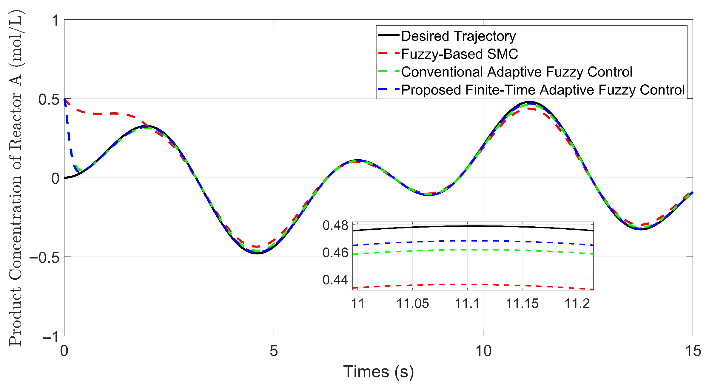
The simulation results are presented in Figure 2, Figure 3, Figure 4, Figure 5 and Figure 6. Figure 2 depicts the tracking error response curves. The total error under the proposed method converges to a neighborhood of $0.01$ within $0.37$ s, which is faster than that of conventional adaptive fuzzy control within $0.46$ s and fuzzy-based SMC within $1.90$ s. Additionally, it can be observed that the error of the proposed method is smaller compared to other methods. Particularly in the stable phase after error convergence, the error fluctuation amplitude of the proposed method is smoother. This result clearly demonstrates that the proposed method enhances the convergence speed and accuracy. In Figure 3, the comparison of tracking performance between the system output $x_1$ and the reference trajectory $y_d$ confirms the controller’s effectiveness. The finite-time strategy achieves superior tracking accuracy, with the output trajectory adhering more closely to the reference signal than those of the other two methods.

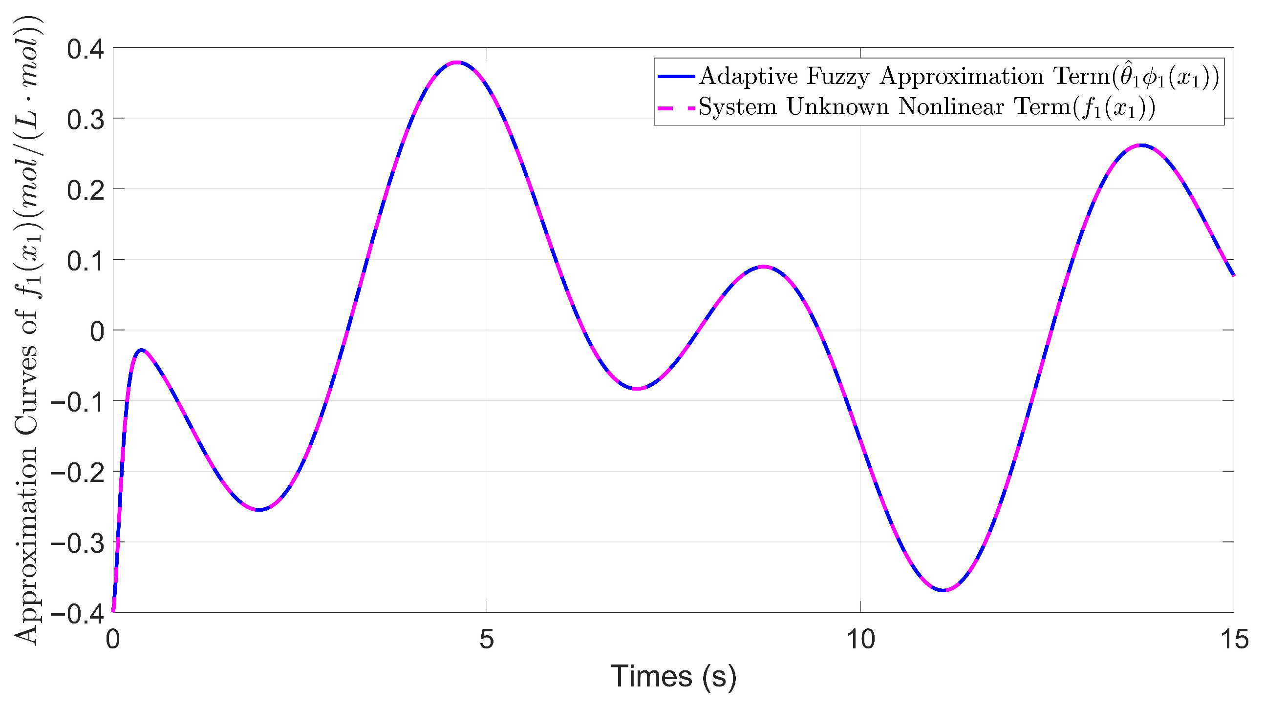
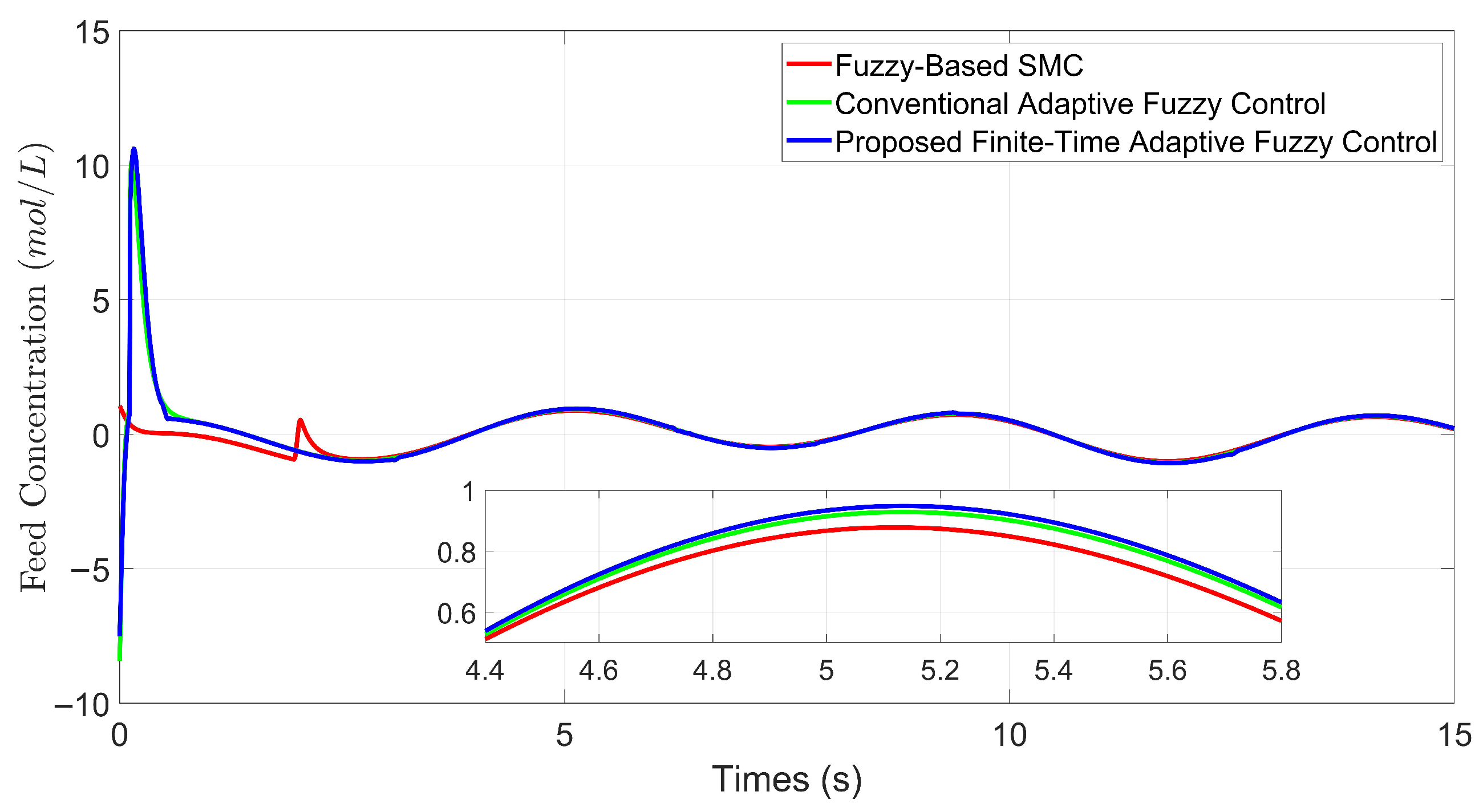
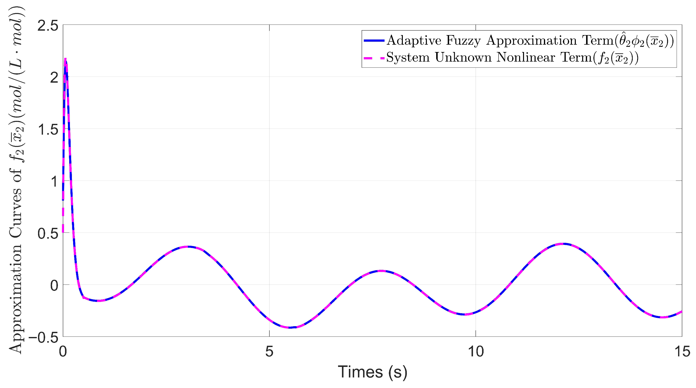
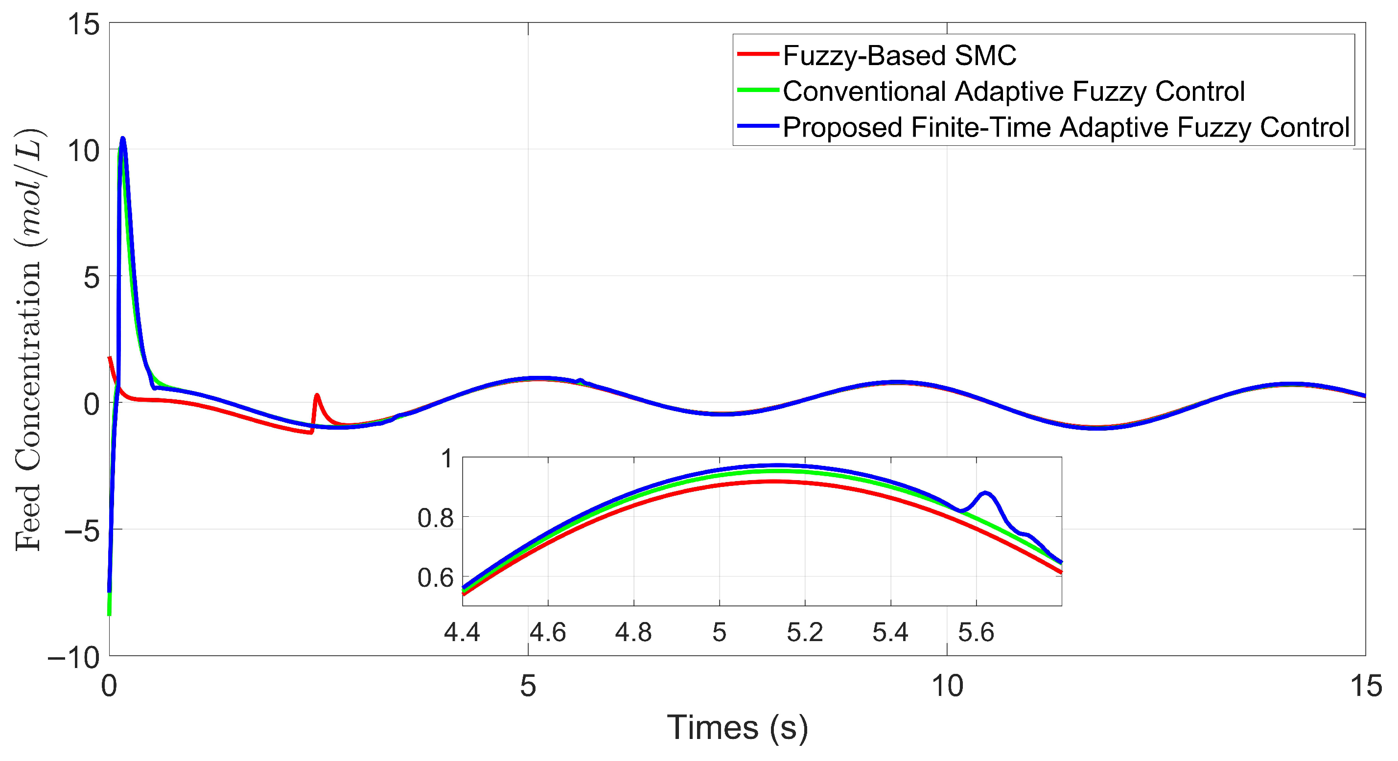
For the estimation of uncertain nonlinear terms, Figure 4 and Figure 5 present the approximation processes of $f_1(·)$ and $f_2(·)$ using FLSs optimized by the GD algorithm with Armijo line search. The results reveal that the system can rapidly and accurately approximate the unknown nonlinear functions when using the proposed method. As shown in Figure 6, the proposed controller exhibits more aggressive compensation during transients, leading to a slightly higher peak magnitude, which is a typical trade-off associated with achieving finite-time convergence.

The simulation results are in complete agreement with the theoretical analyses, thereby demonstrating the proposed method’s advantages in terms of tracking accuracy and convergence speed.

5.2. Example 2: Comparative Analysis Under Disturbance Conditions

Robustness against external disturbances is a critical performance requirement for industrial two-stage CSTR systems, such as feed composition fluctuations and flow rate perturbations. To verify the robustness of the proposed control strategy under disturbances, this section introduces time-varying external disturbances into the model. The disturbances are designed to simulate typical industrial perturbations. These disturbances are designed to simulate typical industrial perturbations. Specifically, the disturbance affecting the concentration dynamics of reactor A is defined as $d_1=-0.5sin\left(0.1t\right)$ mol/L, while the disturbance acting on reactor B is expressed as $d_2=0.2cos\left(0.1t\right)$ mol/L.

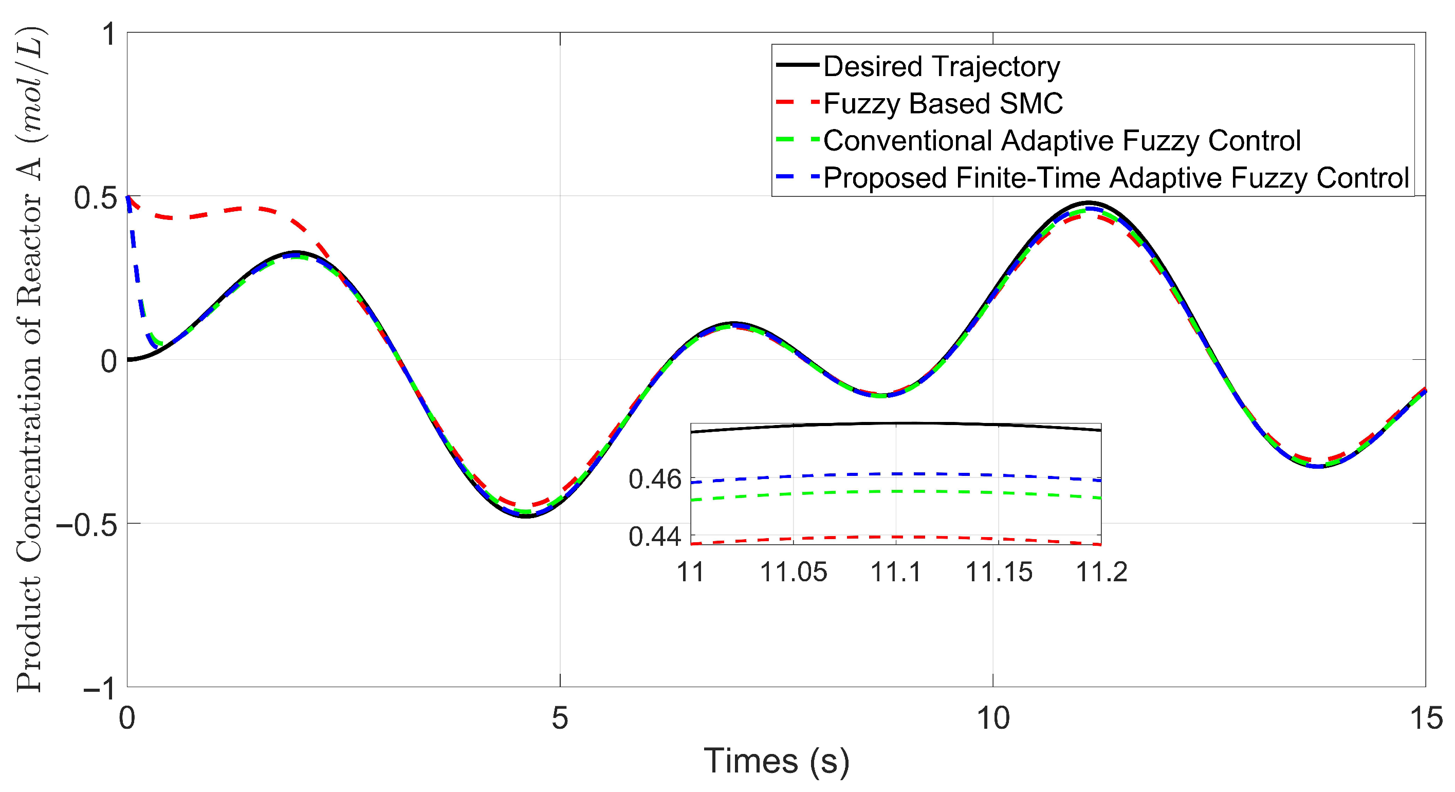
The dynamic response curves of the three control methods under disturbances are presented in Figure 7, Figure 8, Figure 9, Figure 10 and Figure 11, and their quantitative performance metrics are summarized in

Table 3. Performance comparison of different control methods under disturbance conditions.

Control Method	Time for Error $<0.01$ (s)	RMSE (${10}^{-3}$)	IAE	ITAE
Conventional Adaptive Fuzzy Control	0.75	3.586	0.291084	1.377014
Fuzzy-Based SMC	1.90	8.046	0.780444	2.212526
Proposed Finite-Time Adaptive Fuzzy Control	0.58	3.312	0.218131	1.022666

.

Even in the presence of time-varying external disturbances, the proposed method consistently delivers the best overall performance. The tracking error converges more rapidly, the output trajectory adheres more closely to the reference, and all quantitative indicators are uniformly lower than those of conventional adaptive fuzzy control and fuzzy-based SMC. These results, observed across the full disturbance range considered, substantiate the superior robustness of the proposed approach and its ability to maintain high-precision tracking under perturbations. Where applicable, improvements are also statistically significant, further confirming the reliability of the observed gains.

6. Conclusions

This paper proposes a finite-time adaptive fuzzy control strategy based on the GD algorithm with Armijo line search for a two-stage CSTR system. The designed controller ensures that the system’s states converge to the desired trajectory within a finite time, and its tracking error convergence speed is faster compared with the conventional adaptive fuzzy control and fuzzy-based SMC. The employment of finite-time stability, GD with Armijo line search, and adaptive fuzzy systems provides an effective solution for industrial scenarios requiring rapid convergence and high precision. Future work will focus on developing optimization algorithms with smaller estimation errors and higher convergence speeds, and then applying them to finite-time adaptive fuzzy control systems. From the perspective of engineering application, subsequent work needs to clarify the deployment process of the proposed method in actual industrial scenarios. On this basis, its application can be extended to multi-reactor network systems to improve the overall control performance of complex chemical production processes.

References

1. Brison, A.; Rossi, P.; Derlon, N. Single CSTR can be as effective as an SBR in selecting PHA-storing biomass from municipal wastewater-derived feedstock. Water Res. X 2023, 18, 100165. [Google Scholar] [CrossRef]
2. Czyżniewski, M.; Łangowski, R. An observability and detectability analysis for non-linear uncertain CSTR model of biochemical processes. Sci. Rep. 2022, 12, 22327. [Google Scholar] [CrossRef]
3. Wang, Z.; Zhang, Y.; Li, D. Temperature Optimization Control of CSTR. In Proceedings of the 2020 IEEE International Conference on Information Technology, Big Data and Artificial Intelligence (ICIBA), Chongqing, China, 6–8 November 2020. [Google Scholar]
4. So, G.B.; Jin, G.G. Fuzzy-based nonlinear PID controller and its application to CSTR. Korean J. Chem. Eng. 2018, 35, 819–825. [Google Scholar] [CrossRef]
5. Abadi, A.S.S.; Dehkordi, P.H.; Hajiyan, R.; Kowalik, R. Design and real-time evaluation of a novel observer-based predefined-time controller for the industrial processes. ISA Trans. 2024, 156, 551–564. [Google Scholar] [CrossRef] [PubMed]
6. Zhang, Y.; Li, F.; Gao, S.; Zhao, D.; Yan, X.; Spurgeon, S. Output consensus for interconnected heterogeneous systems via a combined model predictive control and integral sliding mode control with application to CSTRs. Control Eng. Pract. 2024, 153, 106100. [Google Scholar] [CrossRef]
7. Liu, Z.; Zhang, Z.; Lin, W.; Yu, X.; Buccella, C.; Cecati, C. Disturbance Rejection-Based Motion Control of Linear Motors Via Integral Sliding Mode Observer. IEEE Trans. Ind. Electron. 2025, 72, 3061–3071. [Google Scholar] [CrossRef]
8. Xie, S.; Xie, Y.; Gui, W.; Yang, C. Weighted-coupling CSTR modeling and model predictive control with parameter adaptive correction for the goethite process. J. Process Control 2018, 68, 254–267. [Google Scholar] [CrossRef]
9. Wang, G.; Jia, Q.-S.; Qiao, J.; Bi, J.; Zhou, M. Deep learning-based model predictive control for continuous stirred-tank reactor system. IEEE Trans. Neural Netw. Learn. Syst. 2020, 32, 3643–3652. [Google Scholar] [CrossRef] [PubMed]
10. Tofighi, S.R.; Bayat, F.; Merrikh-Bayat, F. Robust feedback linearization of an isothermal continuous stirred tank reactor: H mixed-sensitivity synthesis and DK-iteration approaches. Trans. Inst. Meas. Control 2017, 39, 344–351. [Google Scholar] [CrossRef]
11. Yazdi, M.B.; Jahed-Motlagh, M. Stabilization of a CSTR with two arbitrarily switching modes using modal state feedback linearization. Chem. Eng. J. 2009, 155, 838–843. [Google Scholar] [CrossRef]
12. Mathew, E.; Pawar, T.; Jaganatha Pandian, B. Control of a Coupled CSTR Process using MRAC-MIT Rule. In Proceedings of the 2019 Innovations in Power and Advanced Computing Technologies (i-PACT), Vellore, India, 22–23 March 2019; pp. 1–5. [Google Scholar]
13. Cao, L.; Yao, D.; Li, H.; Meng, W.; Lu, R. Fuzzy-based dynamic event triggering formation control for nonstrict-feedback nonlinear MASs. Fuzzy Sets Syst. 2023, 452, 1–22. [Google Scholar] [CrossRef]
14. Meda-Campaña, J.A.; Rodríguez-Manzanarez, R.A.; Ontiveros-Paredes, S.D.; de Jesús Rubio, J.; Tapia-Herrera, R.; Hernández-Cortés, T.; Obregón-Pulido, G.; Aguilar-Ibáñez, C. An algebraic fuzzy pole placement approach to stabilize nonlinear mechanical systems. IEEE Trans. Fuzzy Syst. 2021, 30, 3322–3332. [Google Scholar] [CrossRef]
15. Ma, M.; Wang, T.; Qiu, J.; Karimi, H.R. Adaptive Fuzzy Decentralized Tracking Control for Large-Scale Interconnected Nonlinear Networked Control Systems. IEEE Trans. Fuzzy Syst. 2021, 29, 3186–3191. [Google Scholar] [CrossRef]
16. Qiu, J.; Ma, M.; Wang, T. Event-Triggered Adaptive Fuzzy Fault-Tolerant Control for Stochastic Nonlinear Systems via Command Filtering. IEEE Trans. Syst. Man Cybern. Syst. 2022, 52, 1145–1155. [Google Scholar] [CrossRef]
17. Li, D.; Li, D. Adaptive tracking control for nonlinear time-varying delay systems with full state constraints and unknown control coefficients. Automatica 2018, 93, 444–453. [Google Scholar] [CrossRef]
18. Li, S.; Ahn, C.K.; Guo, J.; Xiang, Z. Neural-network approximation-based adaptive periodic event-triggered output-feedback control of switched nonlinear systems. IEEE Trans. Cybern. 2020, 51, 4011–4020. [Google Scholar] [CrossRef]
19. Liang, H.; Chen, L.; Pan, Y.; Lam, H.K. Fuzzy-based robust precision consensus tracking for uncertain networked systems with cooperative–antagonistic interactions. IEEE Trans. Fuzzy Syst. 2022, 31, 1362–1376. [Google Scholar] [CrossRef]
20. López-Estrada, F.R.; Astorga-Zaragoza, C.M.; Theilliol, D.; Ponsart, J.C.; Valencia-Palomo, G.; Torres, L. Observer synthesis for a class of Takagi–Sugeno descriptor system with unmeasurable premise variable. Application to fault diagnosis. Int. J. Syst. Sci. 2017, 48, 3419–3430. [Google Scholar] [CrossRef]
21. Arifi, A.; Bouallègue, S. Takagi–Sugeno fuzzy-based approach for modeling and control of an activated sludge process. Int. J. Dyn. Control 2024, 12, 3123–3138. [Google Scholar] [CrossRef]
22. Liu, L.; Liu, Y.-J.; Tong, S. Fuzzy-Based Multierror Constraint Control for Switched Nonlinear Systems and Its Applications. IEEE Trans. Fuzzy Syst. 2019, 27, 1519–1531. [Google Scholar] [CrossRef]
23. Chen, Y.F.; Tang, B.; Liu, Q.H. Adaptive fixed-time fuzzy control for delayed recycling continuous stirred tank reactor with asymmetric time-varying full-state constraints. J. Frankl. Inst. 2025, 362, 107410. [Google Scholar] [CrossRef]
24. Kang, S.; Liu, P.X.; Wang, H. Adaptive Fuzzy Finite-Time Command Filtering Control for Flexible-Joint Robot Systems Against Multiple Actuator Constraints. IEEE Trans. Circuits Syst. II Express Briefs 2023, 70, 4554–4558. [Google Scholar] [CrossRef]
25. Qiu, J.; Ma, M.; Wang, T.; Gao, H. Gradient descent-based adaptive learning control for autonomous underwater vehicles with unknown uncertainties. IEEE Trans. Neural Netw. Learn. Syst. 2021, 32, 5266–5273. [Google Scholar] [CrossRef]
26. Yang, X.; Zheng, X. Gradient descent algorithm-based adaptive NN control design for an induction motor. IEEE Trans. Syst. Man Cybern. Syst. 2019, 51, 1027–1034. [Google Scholar] [CrossRef]
27. Zhao, J.; Li, X.; Yu, X.; Wang, H. Finite-time cooperative control for bearing-defined leader-following formation of multiple double-integrators. IEEE Trans. Cybern. 2022, 52, 13363–13372. [Google Scholar] [CrossRef] [PubMed]
28. Li, Y.; Li, K.; Tong, S. Reinforcement learning-based adaptive finite-time performance constraint control for nonlinear systems. IEEE Trans. Syst. Man Cybern. Syst. 2024, 54, 1335–1344. [Google Scholar] [CrossRef]
29. Zhao, G.-H.; Liu, S.J. Decentralized adaptive finite-time stabilization for a class of non-local Lipschitzian large-scale stochastic nonlinear systems. Automatica 2025, 171, 111900. [Google Scholar] [CrossRef]
30. Li, R.; Jin, F.F. Finite-time stabilization output-feedback control of Schrödinger’s equation. J. Process Control 2024, 140, 103258. [Google Scholar] [CrossRef]
31. Bhat, S.P.; Bernstein, D.S. Continuous finite-time stabilization of the translational and rotational double integrators. IEEE Trans. Autom. Control 2002, 43, 678–682. [Google Scholar] [CrossRef]
32. Bhat, S.P.; Bernstein, D.S. Finite-time stability of continuous autonomous systems. SIAM J. Control Optim. 2000, 38, 751–766. [Google Scholar] [CrossRef]
33. Wang, H.; Yu, W.; Ren, W.; Lü, J. Distributed adaptive finite-time consensus for second-order multiagent systems with mismatched disturbances under directed networks. IEEE Trans. Cybern. 2021, 51, 1347–1358. [Google Scholar] [CrossRef]
34. Li, D.; Wang, D.; Liu, L.; Gao, Y. Adaptive finite-time tracking control for continuous stirred tank reactor with time-varying output constraint. IEEE Trans. Syst. Man Cybern. Syst. 2021, 51, 5929–5934. [Google Scholar] [CrossRef]
35. Sang, H.; Wang, P.; Zhao, Y.; Nie, H.; Fu, J. Input–Output Finite-Time Stability for Switched T–S Fuzzy Delayed Systems with a Time-Dependent Lyapunov–Krasovskii Functional Approach. IEEE Trans. Fuzzy Syst. 2023, 31, 3823–3837. [Google Scholar] [CrossRef]
36. Huang, J.; Wen, C.; Wang, W.; Song, Y.D. Design of adaptive finite-time controllers for nonlinear uncertain systems based on given transient specifications. Automatica 2016, 69, 395–404. [Google Scholar] [CrossRef]
37. Yang, Y.; Hua, C.; Guan, X. Adaptive fuzzy finite-time coordination control for networked nonlinear bilateral teleoperation system. IEEE Trans. Fuzzy Syst. 2013, 22, 631–641. [Google Scholar] [CrossRef]
38. Wang, F.; Chen, B.; Liu, X.; Lin, C. Finite-time adaptive fuzzy tracking control design for nonlinear systems. IEEE Trans. Fuzzy Syst. 2017, 26, 1207–1216. [Google Scholar] [CrossRef]
39. Li, D.; Wang, Y.; Liu, Y.-J.; Liu, L. IBLFs-based adaptive fuzzy control for Continuous Stirred Tank Reactors with full state constraints and actuator faults. J. Process Control 2023, 124, 14–24. [Google Scholar] [CrossRef]
40. Zhu, Z.; Xia, Y.; Fu, M. Attitude stabilization of rigid spacecraft with finite-time convergence. Int. J. Robust Nonlinear Control 2011, 21, 686–702. [Google Scholar] [CrossRef]
41. Bruckner, A.M.; Bruckner, J.B.; Thomson, B.S. Problems in Real Analysis: Advanced Calculus on the Real Axis; Springer: New York, NY, USA, 2008; pp. 294–300. [Google Scholar]
42. Qian, C.; Lin, W. Non-Lipschitz continuous stabilizers for nonlinear systems with uncontrollable unstable linearization. Syst. Control Lett. 2001, 42, 185–200. [Google Scholar] [CrossRef]
43. Yan, X.; Chen, M.; Feng, G.; Wu, Q.; Shao, S. Fuzzy Robust Constrained Control for Nonlinear Systems with Input Saturation and External Disturbances. IEEE Trans. Fuzzy Syst. 2021, 29, 345–356. [Google Scholar] [CrossRef]
44. Liu, L.; Yin, S.; Zhang, L.; Yin, X.; Yan, H. Improved results on asymptotic stabilization for stochastic nonlinear time-delay systems with application to a chemical reactor system. IEEE Trans. Syst. Man Cybern. Syst. 2017, 47, 195–204. [Google Scholar] [CrossRef]
45. Wang, L.X. Fuzzy systems are universal approximators. In Proceedings of the IEEE International Conference on Fuzzy Systems, San Diego, CA, USA, 8–12 March 1992; pp. 1163–1170. [Google Scholar]
46. Wei, Z.X.; Li, G.Y.; Qi, L.Q. New nonlinear conjugate gradient formulas for large-scale unconstrained optimization problems. Appl. Math. Comput. 2006, 179, 407–430. [Google Scholar] [CrossRef]
47. Karimi, H.; Nutini, J.; Schmidt, M. Linear Convergence of Gradient and Proximal-Gradient Methods Under the Polyak-Łojasiewicz Condition. In Proceedings of the European Conference on Machine Learning and Knowledge Discovery in Databases, Riva del Garda, Italy, 19–23 September 2016; Springer: Berlin/Heidelberg, Germany, 2016; Volume 9851, pp. 795–811. [Google Scholar]
Figure 1. Two-stage continuous stirred tank reactor system.
Electronics 14 04069 g001
Figure 2. Concentration tracking error under nominal conditions.
Electronics 14 04069 g002
Figure 3. Product concentration of reactor A and desired concentration trajectory under nominal conditions.
Electronics 14 04069 g003
Figure 4. The unknown nonlinear function f 1 and FLS approximation function θ ^ 1 T ϕ 1 ( x 1 ) under nominal conditions.
Electronics 14 04069 g004
Figure 5. The unknown nonlinear function f 2 and FLS approximation function θ ^ 2 T ϕ 2 ( x 2 ) under nominal conditions.
Electronics 14 04069 g005
Figure 6. The feed concentration of the two-stage CSTR system under nominal conditions.
Electronics 14 04069 g006
Figure 7. Concentration tracking error under time-varying external disturbances.
Electronics 14 04069 g007
Figure 8. Product concentration of reactor A and desired concentration trajectory under time-varying external disturbances.
Electronics 14 04069 g008
Figure 9. The unknown nonlinear function f 1 and FLS approximation function θ ^ 1 T ϕ 1 ( x 1 ) under time-varying external disturbances.
Electronics 14 04069 g009
Figure 10. The unknown nonlinear function f 2 and FLS approximation function θ ^ 2 T ϕ 2 ( x 2 ) under time-varying external disturbances.
Electronics 14 04069 g010
Figure 11. The feed concentration of the two-stage CSTR system under time-varying external disturbances.
Electronics 14 04069 g011