Transfer Entropy-Based Causal Inference for Industrial Alarm Overload Mitigation

Abstract

In tightly coupled Industrial Control Systems (ICS), abnormal disturbances often propagate throughout the process, triggering a large number of time-correlated alarms that exceed the handling capacity of the operator. Consequently, a key challenge is how to leverage the directional and temporal characteristics of disturbance propagation to alleviate alarm overload. This paper proposes a delay-sensitive causal inference approach for industrial alarm analysis to address this problem. On the one hand, time delay estimation is introduced to precisely align the responses of two sensor sequences to disturbances, thereby improving the accuracy of causal relationship identification in the temporal domain. On the other hand, a multi-scale subgraph fusion strategy is designed to address the inconsistency in causal strength caused by disturbances of varying intensities. By integrating significant causal subgraphs from multiple scenarios into a unified graph, the method reveals the overall causal structure among alarm variables and provides guidance for alarm mitigation. To validate the proposed method, a case study is conducted on the Tennessee Eastman Process. The results demonstrate that the approach identifies causal relationships more accurately and reasonably and can effectively reduce the number of alarms by up to 51.6%.

1. Introduction

In Industrial Control Systems, multiple highly coupled control loops operate in coordination to perform sophisticated closed-loop control tasks. These loops ensure that key physical and chemical variables, such as temperature, pressure, flow rate, and concentration remain within specified ranges, thereby maintaining the continuity and safety of production operations [1,2]. However, the strong interdependence among process variables, which underpins these control strategies, also facilitates the rapid amplification and propagation of disturbances. Such disturbances can cascade through the process chain and affect multiple subsystems, often triggering a chain reaction. A single sensor fault or a targeted cyber attack may not only cause localized disruption, but also lead to non-periodic, cross-variable anomalies that exhibit strong inter-variable correlations. For example, a malfunctioning control valve might cause deviations in downstream readings such as temperature, pressure, and concentration, resulting in the rapid activation of multiple alarms in a short period of time [3,4].

Due to the limited understanding of alarm interrelationships, operators are often overwhelmed by a flood of alarms, many of which are triggered by the same disturbance. To address alarm overload, it is crucial to uncover the underlying causal relationships among alarms, particularly by identifying upstream variables that trigger cascades. This allows for operators to focus on a few critical alarms rather than being distracted by a large number of derivative alarms. Consequently, discovering causal structures has become a key research issue for enhancing both the efficiency and the reliability of alarm management.

In general, causal inference aims to assess whether one event exerts a direct influence on another [5]. When applied to industrial alarm analysis, causal inference methods can help to reveal how sensor variables depend on each other. They can also uncover hidden propagation pathways that are difficult to detect using traditional process knowledge. By mapping these causal relationships, operators can quickly trace upstream and downstream relationships within large alarm sequences. This process greatly reduces the complexity of alarm management and lightens the cognitive workload of operators. However, existing data-driven or structure-based causal discovery methods remain limited in industrial contexts due to two fundamental challenges.

First, the misalignment of response delays between variables in ICSs can significantly undermine the accuracy of causal inference. Although some existing methods consider time-lag effects, they typically assume fixed delays or employ non-fixed delays without clear physical interpretability. In ICSs, causal responses are inherently influenced by factors such as physical distance, control loop latency, and actuator inertia, resulting in dynamic time lags [2]. When such dynamics are modeled statically or without proper interpretation, the resulting mappings between disturbance and response sequences become misaligned. In that case, variables that have already responded may be confused with those that have not yet reacted. This misalignment may introduce spurious causal links or obscure real but delayed causal relations, ultimately degrading the reliability and accuracy of causal inference.

Second, multi-source disturbances in ICSs create different levels of causal strength among variables, which challenges the completeness of causal identification. During operation, control loops often experience disturbances of varying magnitudes and at different times. These conditions generate heterogeneous causal patterns. Weaker disturbances may cause only subtle causal effects, which can be easily overshadowed by dominant influences from stronger anomalies. As a result, the system’s overall causal landscape becomes unbalanced. This imbalance can obscure the full landscape of causal interactions, leading to incomplete representations of the underlying propagation structure.

To overcome these challenges, this paper proposes a novel alarm relation analysis framework based on modified transfer entropy. The innovation of the framework lies in two aspects: (i) Dynamic time delays are explicitly incorporated into the transfer entropy computation, ensuring accurate alignment of cause–effect sequences. Compared with static delay settings [6,7,8,9] and unexplained delay selection methods [10,11,12,13,14,15], this design achieves higher accuracy and interpretability in causal inference. (ii) A multi-scale subgraph fusion strategy is developed to distinguish and integrate causal relationships across different disturbance levels. Unlike existing methods that focus only on single-scenario relationships [6,10,11,12,13,14,16,17,18], the proposed method captures a richer set of causal relationships with improved accuracy and robustness. By fusing local causal fragments into a global propagation structure, the method also provides clear practical advantages in alarm management. In particular, the framework enables operators to filter redundant alarms and reduce alarm flooding, thereby supporting safer and more efficient operation of industrial processes.

The main contributions of this paper are as follows:

• We propose a method to mitigate industrial alarm overload. The method relies on causal inference and identifies causal relationships through precise disturbance–response mapping, which enhances the accuracy of alarm processing.
• We develop a multi-scale subgraph fusion strategy that discriminates between causal influences induced by strong and weak disturbances, effectively bridging the relational boundaries caused by disturbance magnitude.
• We validate our method on the Tennessee Eastman Process, demonstrating superior causal inference capability and significant reduction in alarm volume.

The rest of this paper is organized as follows: Section 2 focuses on introducing existing methods of causal inference and summarizing shortcomings. Section 3 presents the proposed method, which concludes the overall framework and details of our method. A case study based on the Tennessee Eastman Process is performed in Section 4. And Section 5 compares some existing methods with ours and discusses the results. Finally, the work is concluded in Section 6.

2. Related Work

Causal inference is a fundamental technique for large-scale alarm analysis. It provides an efficient analytical framework, particularly for industrial systems characterized by complex technological processes and periodic operations. Some previous research traditionally relied on qualitative information about process mechanisms and expert knowledge to infer relationships [19]. However, such approaches are limited by system scale and cannot be easily generalized to other industrial domains. In recent years, data-driven approaches have compensated for this shortcoming to some extent. With the ability to mine causality, data-driven approaches can provide dynamic information hidden in a state of flux when expert knowledge is limited.

According to the classification in [20], data-driven causal inference methods can be divided into two categories: linear and nonlinear. Among them, Granger causality analysis and transfer entropy, as typical methods of the mentioned categories, are also the two most commonly used methods in causal inference [21]. Granger causality relies on assuming a linear vector autoregressive model to verify the effect of one sequence on the future occurrence of a term in another sequence [22]. However, researchers have found that Granger causality has great limitations, which is reflected in the nonlinear causality of most variables [23,24]. The linearity requirement is undoubtedly ideal and strict for highly complex industrial control systems that contain monitored variables. Previous studies [25] have extended the applicability of Granger causality by relaxing nonlinear assumptions. Nevertheless, the results obtained from transfer entropy are generally more accurate and more visually interpretable [26].

In contrast, the transfer entropy is more applicable to the analysis of industrial alarms as a non-parametric causality inference method [16]. Therefore, this paper utilizes the transfer entropy-based approach for causal inference of industrial alarms, which is the focus of the following related work. To improve clarity and visualization, we compare our method with existing approaches in

Table 1. Comparison of related work.

	Main Techniques	Dynamic Alignment	Interpretability	Causal Graph
[6]	Modified transfer entropy	No	Yes	Yes
[16]	Modified transfer entropy	Yes	Yes	No
[17]	Modified transfer entropy	Yes	No	Yes
[18]	Transfer entropy & Conditional mutual information	Yes	No	Yes
[10]	Transfer entropy & Granger casuality	No	No	Yes
[11]	Modified transfer entropy	Yes	No	Yes
[12]	Transfer entropy	Yes	No	No
[7]	Transfer entropy & Bayesian networks	No	No	Yes
[13]	Modified transfer entropy & Bayesian networks	Yes	No	No
[14]	Transfer entropy & Bayesian networks	Yes	No	Yes
[15]	Modified transfer entropy	Yes	No	Yes
[8]	Modified transfer entropy	No	No	Yes
[9]	Modified transfer entropy	No	No	Yes
[27]	Renyi transfer entropy	No	No	No
Ours	Modified transfer entropy	Yes	Yes	Yes

. The comparison highlights their main techniques, the treatment of dynamic time delay, the interpretability of parameter selection, and whether a causality graph is provided.

For the transfer entropy calculation method, some studies [6,11,17] made improvements. Bauer et al. [6] introduced the concept of prediction horizon to compensate for the neglect of time delay of the original transfer entropy calculation method. They analyzed how parameter selection affects significance levels and proposed strategies for more reasonable parameter combinations. Based on this work, Shu et al. [17] incorporated sequence coherence before and after the delay to further improve transfer entropy estimation. However, Zhu et al. [11] argued that fixed delay intervals could not capture the dynamics of most real-world processes. They therefore enhanced the adaptability of the present-sequence intervals, making transfer entropy more responsive to varying temporal dependencies.

Jizba et al. [27] extended the conventional Shannon entropy-based TE to analyze coupled time sequences generated from known dynamic systems. Their approach enabled the detection of causal directions within these sequences. Zhang et al. [16] proposed a new framework to improve the calculation of transfer entropy, using the information granulation as a prior step to determine the window length for performing data compression. It is worth noting that this method can reduce the computational complexity significantly, but may introduce the risk of losing useful information. For early fault diagnosis, Qi et al. [15] proposed a Dynamic Data Stream Transfer Entropy (DSTE) algorithm. This algorithm incorporates data stream techniques to support continuous data updating and applies clustering methods for data compression, thereby improving the efficiency of causality analysis. Ekhlasi et al. [8] refined the measurement of causal strength by counting the number of significant connections between repeated segments during the computation of transfer entropy. And Falkowski et al. [9] proposed an improved transfer entropy method from the perspective of probability density functions. By selecting the best-fitting distribution from Cauchy, $\alpha$-stable, Laplace, Huber, and t-location scale distributions, they enhanced causality detection in multiloop control systems and demonstrated the influence of distribution selection on the performance of transfer entropy.

Several studies have also integrated transfer entropy with other methods to enhance causal inference. It is common to combine transfer entropy and Bayesian network to infer causality. Luo et al. [13] eliminated the effect of the common cause variable and utilized a greedy search algorithm to derive the relational structure. Considering the self-interference of industrial variables, Meng et al. [7] proposed a scoring function for Bayesian network structures based on family transfer entropy. This approach effectively eliminated the impact of self-interference during network evaluation. Conversely, De Abreu et al. [14] used transfer entropy results to determine the input order of a Bayesian structure learning algorithm. They introduced virtual nodes to remove the indirect relationship by judging the delay, while Su et al. [18] proposed a hybrid method based on the transfer entropy and modified conditional mutual information, which used conditional mutual information to distinguish between direct and indirect relationships.

In addition, Hu et al. [10] applied the transfer entropy and Granger causality to different scenarios of causal inference. And they extracted alarm association variables based on process information to reduce the number of involved process variables. Similar to the paper by [10], Suresh et al. [12] combined a data-driven causal graph with a process model-based approach so as to identify causality more accurately. Specifically, they first classified variables hierarchically using structural information from flowsheets and then applied transfer entropy to determine their relationships. However, the requirement of structural information will limit the application scenarios of this method.

Despite these advances, most of the existing approaches face additional limitations when applied to complex industrial contexts. First, the scalability of these methods to high-dimensional multivariate systems is limited, since the computational cost of joint probability estimation grows rapidly with the number of variables. Second, nonlinear interactions that are common in industrial processes are often not sufficiently captured by traditional entropy-based measures with fixed assumptions on distribution or delay structure. Third, only some of them consider the influence of dynamic time delays on sequence mapping [11,12,13,14,15,17,18]. Although these methods adapt delay values by maximizing transfer entropy, this strategy can lead to spurious correlations if the response alignment between sequences is inaccurate. Finally, most studies assume a single disturbance source, overlooking the varying causal strengths that arise in multi-disturbance industrial systems.

To address these issues, we propose a method that dynamically estimates the time delay to accurately align the response timing between two sequences during transfer entropy computation, thereby avoiding the introduction of spurious causal relationships and enhancing the interpretability of the analysis. Finally, the causal analysis results are visualized by generating and integrating subgraphs under multiple disturbance scenarios, which assists operators in improving efficiency when responding to large volumes of alarms.

3. Proposed Method

As a concise way to represent causal relationships among multiple alarm variables, the causal graph illustrates how one variable can influence another through the transitive nature of the control process. This graph is constructed from transfer entropy calculations, where each node represents an alarm variable and each directed edge indicates a causal relationship between variables.

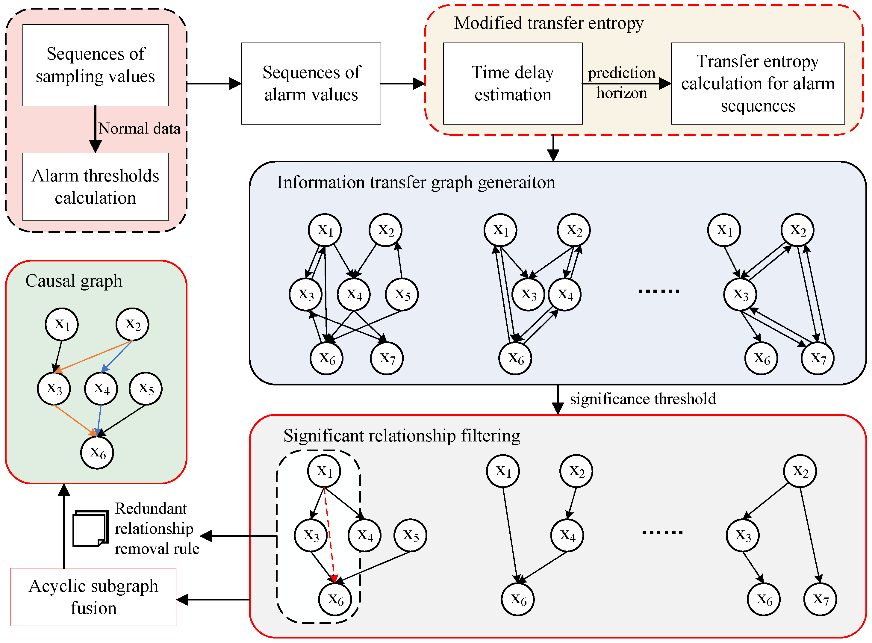
To provide an overview of the proposed framework, Figure 1 outlines the key steps involved in generating the causal graph and the logical connections between them. The core idea can be summarized in three stages: First, the corrected transfer entropy is applied to estimate potential dependencies among variables. Second, significance thresholds and a removal rule are introduced to filter out spurious relationships. Finally, the significant causal links identified from all subgraphs are integrated to form the complete causal graph.

3.1. Introduction of Transfer Entropy

Transfer entropy is derived from the information entropy [28]. Information entropy was introduced to measure the relationship between uncertainty and probability of occurrence. Based on the principle that low-probability events can convey more information, the lower the probability is, the greater the uncertainty is and the higher the information entropy is. However, the information entropy is an independent measure, and thus cannot help to describe the information transferred between two events or sequences. Therefore, Schreiber et al. [29] proposed the transfer entropy based on the definition of the information entropy to measure the amount of information transferred from variable y to x as Equation (1).

$$\begin{array}{c}\hfill t(y\to x)=\sum _{x_{i+1},x_i^{\left(k\right)},y_i^{\left(l\right)}}(p(x_{i+1},x_i^{\left(k\right)},y_i^{\left(l\right)})\\ \hfill log{\displaystyle \frac{p(x_{i+1}\mid x_i^{\left(k\right)},y_i^{\left(l\right)})}{p(x_{i+1}\mid x_i^{\left(k\right)})}})\end{array}$$

(1)

where $x_{i+1}$ and $x_i^{\left(k\right)}=[x_i,x_{i-1},\cdots ,x_{i-k+1}]$ represent the value of x at time $i+1,i,\cdots ,i-k+1$, respectively. $y_i^{\left(l\right)}=[y_i,y_{i-1},\cdots ,y_{i-l+1}]$ represents the value of y at time $i,\cdots ,i-l+1$. $p(x_{i+1},x_i^{\left(k\right)},y_i^{\left(l\right)})$ denotes the joint probability, $p(x_{i+1}\mid x_i^{\left(k\right)},y_i^{\left(l\right)})$ and $p(x_{i+1}\mid x_i^{\left(k\right)})$ denote the conditional probability, and k and l indicate the dimensions of x and y, respectively.

The modified transfer entropy proposed by Bauer et al. [6] considers time difference a step further. The prediction horizon they introduced, h, enables the transfer entropy to describe the sequence lag. The $x_{i+1}$ was represented as $x_{i+h}$ to parameterize the time difference.

Based on the research of Bauer et al. [6], Shu et al. [17] assumed that the sequence strictly followed the Markov property. In other words, the values of variables in the same sequence are only relevant to their previous moment. Therefore, the $x_i^{\left(k\right)}$ was replaced by $x_{i+h-1}^{\left(k\right)}$.

3.2. Modified Transfer Entropy Based on Time Delay Estimation

The three adjustable parameters are $k,l$, and h. k and l determine the dimension of the sequence x and y extracted at the current moment and affect the statistics of the joint and conditional probabilities. However, h determines the position of the sequence x and y that we extracted for the uncertainty calculation. For delay-sensitive sequences, the choice of the prediction horizon h greatly affects the results of the transfer entropy. To obtain a more accurate transfer entropy, we optimize the method for determining h. The cross-correlation function (CCF) is usually used in signal processing to estimate the delay between two signals [30,31]. In our method, we have innovatively introduced the CCF into the processing of alarm sequences to optimize the calculation of transfer entropy.

CCF reflects the degree of mutual matching between two sequences in a relative position. In practice, the CCF of two sequences is equal to the linear convolution of the first sequence after folding and conjugating with the second sequence. As the alarm sequence is a discrete sequence, the CCF can be expressed as Equation (2):

$$R\left(\tau \right)=\sum _{t=-\infty }^{+\infty }x\left(t\right)·y(t-\tau )$$

(2)

where $\tau$ is the time delay.

When Equation (2) reaches its maximum at $\tau ={\tau }_0$, it indicates that the two sequences are most strongly correlated at ${\tau }_0$. Therefore, the time delay of the two sequences can be derived as the position where the function Equation (2) reaches its maximum. ${\tau }_0$ can be calculated using Equation (3):

$${\tau }_0=argmaxR\left(\tau \right)=argR\left({\tau }_0\right)$$

(3)

The exact time delay estimated by the CCF is assigned to the prediction horizon, h. Thus, the modified transfer entropy in our method is expressed as Equation (4):

$$\begin{array}{c}\hfill t(y\to x)=\sum _{x_{i+{\tau }_0},x_{i+{\tau }_0-1}^{\left(k\right)},y_i^{\left(l\right)}}(p(x_{i+{\tau }_0},x_{i+{\tau }_0-1}^{\left(k\right)},y_i^{\left(l\right)})\\ \hfill log{\displaystyle \frac{p(x_{i+{\tau }_0}\mid x_{i+{\tau }_0-1}^{\left(k\right)},y_i^{\left(l\right)})}{p(x_{i+{\tau }_0}\mid x_{i+{\tau }_0-1}^{\left(k\right)})}})\end{array}$$

(4)

In addition, to illustrate the effectiveness of our improvement, two sequences with obvious time delays are used to show the relationship between transfer entropy and time delay. As shown in Figure 2, y is 4 points ahead of x. Reflecting in the transfer entropy, the value of time delay ${\tau }_0$, which is 4 for the two example sequences, makes $t(y\to x)$ reach the maximum at $h={\tau }_0=4$. The estimation of the time delay significantly enhances the reasonableness of transfer entropy calculation between the two sequences.

3.3. Multi-Scale Significance Relationships Filtering

In scenarios with multiple disturbance sources, using a single global significance threshold for transfer entropy may introduce bias in causal inference. In such cases, strong disturbances may dominate the transfer entropy distribution, thereby overshadowing the weaker but meaningful causal links that arise under milder disturbances. To mitigate this problem, a specific transfer entropy threshold is calculated for each disturbance scenario to reflect the strength of its associated disturbance.

Specifically, for each disturbance scenario, an information transfer subgraph is first constructed. Since transfer entropy is inherently directional, the resulting structure is naturally modeled as a directed graph, formally defined as follows:

Definition 1. 

Let  G = (V,E) be a directed graph, where V = $\{V_i\mid i=1,2,\dots ,n\}$ denotes the set of nodes and E ⊆ V × V represents the set of directed edges between node pairs. In this study, nodes correspond to alarm variables, and edges represent directional causal relationships inferred between them.

It is important to note that during the construction of each information transfer subgraph, no edges are filtered out, regardless of their statistical strength. This design preserves all observed information flows and provides operators with a complete view of the effects between variables for reference.

Algorithm 1 illustrates the construction of an information transfer subgraph for a single-disturbance scenario using the modified transfer entropy method. Applying this procedure to each disturbance scenario results in a set of scenario-specific subgraphs. In detail, the alarm sequences in the dataset are traversed to compute the CCF (lines 1–5). Different sequence pairs are then selected for transfer entropy calculation (lines 7–10), and variable pairs with identified relationships are visualized in the information transfer graph (lines 11–13).

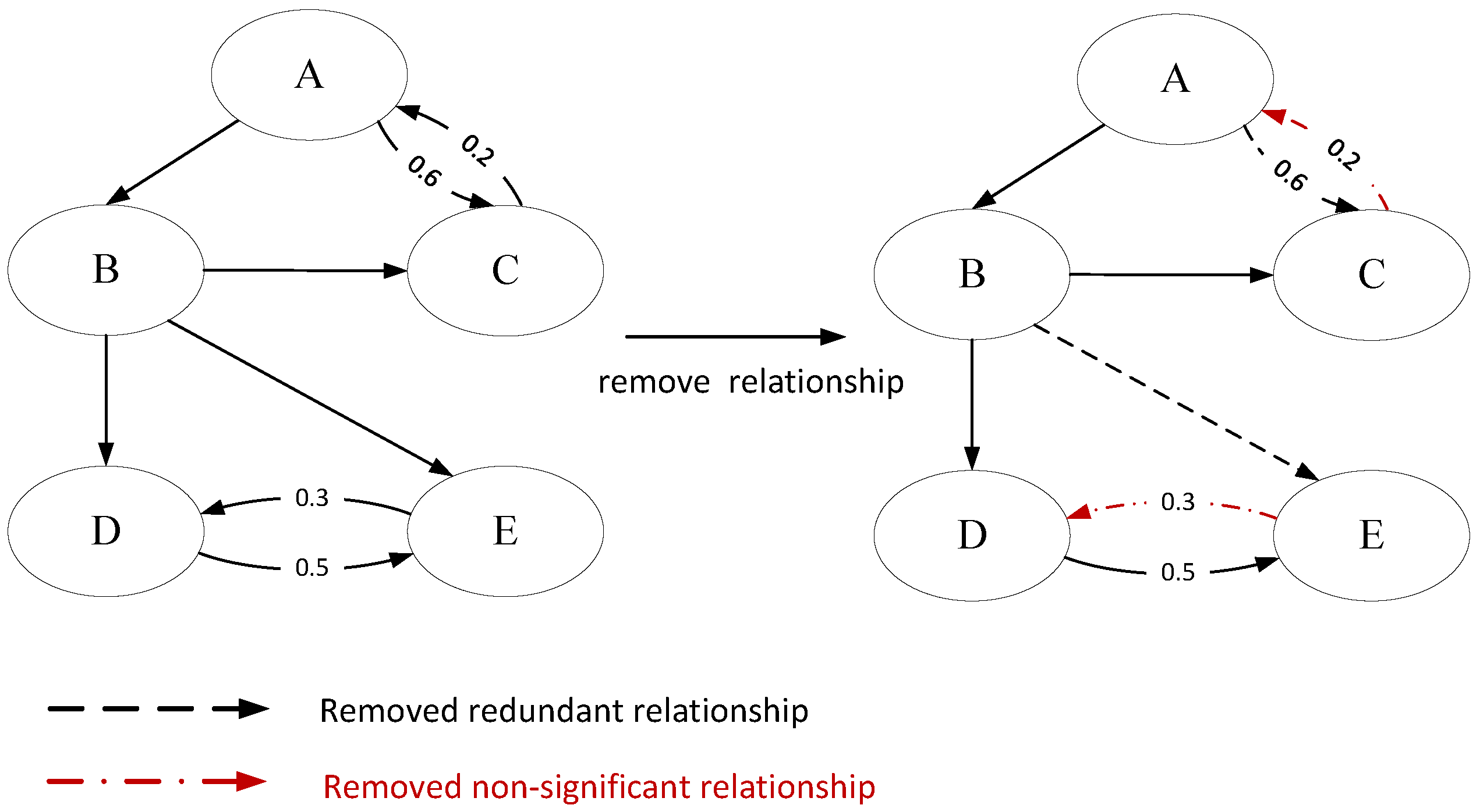
Since transfer entropy is an asymmetric metric, it typically yields two distinct values for each variable pair, depending on the direction of information flow. However, in real-world systems, the true causal relationship between two variables is typically unidirectional. Therefore, our framework preserves only the direction with the higher transfer entropy value, assuming that it represents the dominant flow of information. For example, as illustrated in Figure 3, both $A\to C$ and $C\to A$ (as well as $D\to E$ and $E\to D$) may initially be considered causal hypotheses. However, only the direction with the larger transfer entropy value is retained, while the counterpart with the smaller transfer entropy value is removed. The removed edges are indicated with red dashed lines in Figure 3.

To improve the sensitivity of causal inference under varying disturbance intensities, we further introduce an adaptive significance thresholding strategy based on the transfer entropy distribution. Concretely, we consider D operational scenarios or temporal segments. For each scenario $d\in \{1,2,\dots ,D\}$, we compute a significant transfer entropy threshold tailored to its particular information transfer scale.

Algorithm 1: Generate the information transfer graph

For each source-target variable pair $(y\to x)$ in scenario d, the filtering rule for significant relationships is

$${\displaystyle \frac{t_{y\to x}^{\left(d\right)}-{\mu }_t^{\left(d\right)}}{{\sigma }_t^{\left(d\right)}}}\ge s_{y\to x}^{\left(d\right)}$$

(5)

where ${\mu }_t^{\left(d\right)}$ and ${\sigma }_t^{\left(d\right)}$ denote the mean and standard deviation of all transfer entropy values computed in scenario d, calculated as

$${\mu }_t^{\left(d\right)}={\displaystyle \frac{1}{N_d}}\sum _{i=1}^{N_d}{t}_i^{\left(d\right)}, {\sigma }_t^{\left(d\right)}=\sqrt{{\displaystyle \frac{1}{N_d-1}}\sum _{i=1}^{N_d}{(t_i^{\left(d\right)}-{\mu }_t^{\left(d\right)})}^2}$$

(6)

where $t_i^{\left(d\right)}$ is the i-th transfer entropy value in scenario d, and $N_d$ is the total number of variable pairs in that scenario.

The threshold $s_{y\to x}^{\left(d\right)}$ is determined based on a 90% confidence level in our paper. The adaptive thresholding strategy enhances the model’s sensitivity to scenario variations. It also prevents weak but meaningful causal relationships from being masked by global-scale effects.

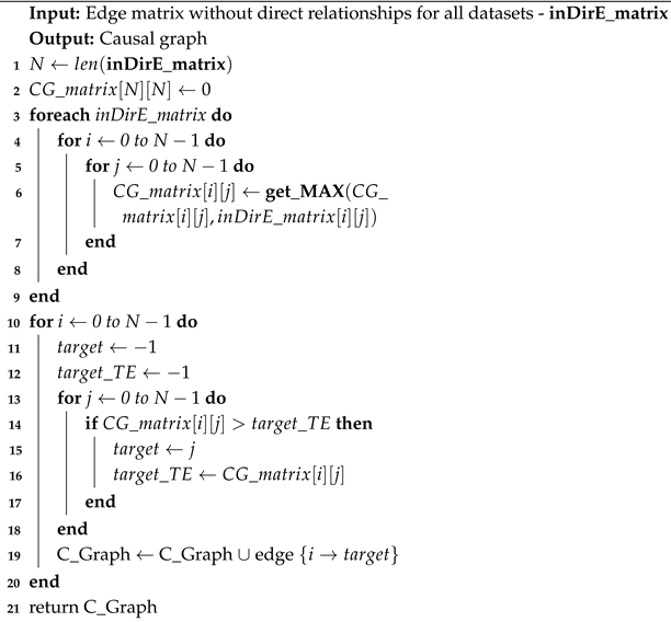
With the aim of filtering significant relationships, Algorithm 2 shows the execution steps. The values in the edge matrix are traversed (lines 3–4). When a transfer entropy value exceeds the threshold, the relationship between the corresponding variables is recorded as significant (lines 5–7). After all significant relationships have been recorded, the maximum principle is applied. Specifically, only the direction with the larger transfer entropy value between two variables is retained as the final significant relationship (lines 8–10).

Algorithm 2: Filter significance relationships

3.4. Acyclic Subgraph Fusion

The significant subgraphs obtained under different disturbance scenarios still lack sufficient global interpretability. To address this issue, we integrate these subgraphs into a comprehensive causal graph that provides more effective guidance for operators when dealing with alarm floods. The motivation for merging subgraphs is inspired by the observation that causal inference often exhibits dependence on the fluctuation of causal strength. In individual scenarios, the inferred relationships may be limited to local variable interactions directly impacted by the disturbance. As the influence weakens near scenario boundaries, relationships among peripheral variables become difficult to capture. Weak long-distance influences often limit causal identification. To address this, we merge significant subgraphs across different scenarios, which allows for causal relationships to be represented in a unified dimension and provides operators with a more comprehensive causal guidance map.

However, merging subgraphs may introduce multiple paths between variable pairs. For example, as shown in Figure 3, there exist two paths from node A to node C: A → B → C and A → C. The path A → B → C captures three types of potential causal links: A → B, B → C, and A → C. We consider that the influence from A to C is implicitly represented in the path A → B → C. Therefore, we remove the direct edge A → C.

This pruning strategy is based on two considerations: (1) The primary goal of this study is to guide operators in mitigating alarm floods using inferred causal relationships. This practical objective informs our edge-pruning policy: retain as many potentially meaningful links as possible to ensure comprehensive and actionable guidance for alarm handling. In this case, we maintain the relationship A → B → C to convey more actionable information. (2) In ICS, causal influence is typically transitive. Both the direct edge A → C and the indirect path A → B → C can be used to suppress unrelated downstream alarms. Therefore, for the purpose of alarm suppression, we do not strictly differentiate between single-step and multi-step causal paths.

In Figure 3, the retained relationships are shown with solid black lines, while the removed relationships are indicated by dashed black lines. Based on this principle, we reconstruct the merged causal graph to more accurately reflect the influence pathways among variables. Algorithm 3 illustrates how this strategy merges significant subgraphs into a unified causal graph. Specifically, the relationship matrices of all subgraphs are traversed, and only the maximum transfer entropy value of each relationship is preserved (lines 3–7). The strongest causal relationship for each variable is then identified (lines 10–18) and represented in the causal graph (line 19).

Once the final causal graph is obtained, operators can focus on downstream alarms that are causally linked to upstream variables that have already triggered alarms, while ignoring unrelated alarms. This approach effectively alleviates the burden of alarm flooding.

Algorithm 3: Generate the causal graph

4. Case Study

Through a case study, we illustrate the implementation of the methodology in this paper using multiple intermediate results. The Tennessee Eastman (TE) process, as a benchmark process for industrial monitoring and control, was selected to support the implementation of the method.

4.1. Tennessee Eastman Chemical Process

The TE process is a typical chemical simulation process consisting of five operating units: the reactor, the condenser, the vapor–liquid separator, the recycle compressor, and the product stripper. The entire process involves 41 measured variables and 12 manipulated variables [32]. The process flow is shown in Figure 4.

To simulate actual faults in the chemical system, the TE process imposes 20 disturbances on multiple variables such as components, temperature, pressure, and valves. In addition to each disturbance providing a dataset of all variables, there is also a dataset of normal conditions that can be used as training data. Each dataset contains 960 samples, and the disturbance is introduced at the 160th.

Following prior research [11,19,22,32], the system is divided into five subsystems: the reactor, condenser, separator, stripper, and compressor subsystems. In order to better demonstrate the effectiveness of our method, the subsystem with a more comprehensive coverage of feed stream will be selected. Equation (7) shows the reaction relationships among the feed streams.

$$\begin{array}{c}\hfill A\left(g\right)+C\left(g\right)+D\left(g\right)\to G\left(liq\right)\\ \hfill A\left(g\right)+C\left(g\right)+E\left(g\right)\to H\left(liq\right)\\ \hfill A\left(g\right)+E\left(g\right)\to F\left(liq\right)\\ \hfill 3D\left(g\right)\to 2F\left(liq\right)\end{array}$$

(7)

According to the analysis reaction relationships, the reactor subsystem is selected as the most affected subsystem. The description of the process variables in this subsystem is given in

Table 2. Process variables used in the Tennessee Eastman process.

Variable	Variable Description
$v_1$	A Feed (stream 1)
$v_2$	D Feed (stream 2)
$v_3$	E Feed (stream 3)
$v_4$	A and C Feed (stream 4)
$v_6$	Reactor feed rate (stream 6)
$v_7$	Reactor pressure
$v_8$	Reactor level
$v_9$	Reactor temperature
$v_{21}$	Reactor cooling water outlet temperature

.

Based on the variables used in our experiment, several typical disturbance scenarios involving these variables are considered for illustration. The description of these disturbance scenarios is shown in

Table 3. Disturbance description in the Tennessee Eastman process.

Disturbance	Disturbance Description
IDV1	Step in A/C feed ratio, B composition constant
IDV2	Step in B composition, A/C ratio constant
IDV6	A feed loss
IDV7	C header pressure loss
IDV9	Random variation in D feed temperature
IDV12	Random variation in condenser cooling water inlet temperature
IDV14	Sticking reactor cooling water valve

.

4.2. Experimental Setup

The proposed method involves two key parameters: the history lengths k and l used in the calculation of transfer entropy. Larger values of k and l correspond to longer historical time series considered in the embedding. In this study, we adopt the same parameter configuration as previous transfer entropy-based alarm sequence analysis studies [13,14,16,18], setting $k=1$ and $l=1$. This choice is based on the following considerations:

(1)

Compared with traditional binary or ternary alarm encodings, the multi-valued alarm sequences used in our study better reflect the directional evolution trend of alarms. Therefore, instead of emphasizing extended history in the embedding space, we focus on extracting information flow at each sampling point, which aligns more closely with the operational logic of industrial alarms.

(2)

Increasing k and l raises the embedding dimension, which significantly increases the computational complexity.

Therefore, to ensure that causal inference can be performed promptly for practical alarm suppression, we adopt the simplest and most widely used parameter configuration.

4.3. Multi-Valued Alarm Processing

Following the data preprocessing strategies adopted in previous studies [6,7,10,13,14,16,18], and considering the hierarchical nature of ICS alarms, the discrete sampling sequences are converted into multi-valued alarm sequences. Furthermore, to better preserve the underlying trend information in the time series, we adopt a five-level alarm encoding rather than ternary representations.

To more realistically simulate the alarm-triggering conditions of chemical processes, four alarm thresholds are defined: High–High (HH), High (H), Low (L), and Low–Low (LL). The basic thresholds for H and L alarms are determined from the training data based on the typical $3\sigma$ principle used in ICSs, while the HH and LL thresholds are obtained by segmenting the overall range of sampled values. This hierarchical thresholding principle affects the trend variations in the discretized sequences; therefore, we adopt the most commonly used practice in industrial control applications. Specifically, the multi-valued alarm sequence can be computed according to Equation (8):

$$A_{\left(t\right)}=\left\{\begin{array}{ccc}\hfill 2& \hfill & \hfill (\mu +3\sigma )+0.5(max-\mu -3\sigma )\le s{v}_{\left(t\right)}\\ \hfill 1& \hfill & \hfill \mu +3\sigma \le s{v}_{\left(t\right)}<(\mu +3\sigma )+0.5(max-\mu -3\sigma )\\ \hfill 0& \hfill & \hfill \mu -3\sigma \le s{v}_{\left(t\right)}<\mu +3\sigma \\ \hfill -1& \hfill & \hfill (\mu -3\sigma )-0.5(\mu -3\sigma -min)\le s{v}_{\left(t\right)}<\mu -3\sigma \\ \hfill -2& \hfill & \hfill s{v}_{\left(t\right)}<(\mu -3\sigma )-0.5(\mu -3\sigma -min)\end{array}\right.$$

(8)

where $A_{\left(t\right)}$ represents the t-th value of the alarm sequence, $s{v}_{\left(t\right)}$ represents the t-th value of the sampled sequence, and $\mu$ and $\sigma$ denote the mean and standard deviation of the sampled values, respectively. $max$ and $min$ represents the maximum and the minimum value of the sampled values, respectively.

In Figure 5, we take the variable $v_{21}$ as an illustrative example to demonstrate the processing of multi-valued alarms. The upper plot shows the trend of the sampled values, while the lower plot presents the corresponding alarm sequence. Given the sampled value at each time step, the alarm level is computed using Equation (8), and the resulting values are then integrated into a complete alarm sequence. Obviously, in contrast to sampled value sequences, multi-valued alarm sequences focus on the outliers that are triggered by disturbances, which enhance the detection of anomaly propagation.

4.4. Information Transfer Graph Generation

Multi-valued alarm sequences are utilized to estimate time delays and compute transfer entropy. For each pair of variables, we estimate the corresponding time delay to guide the selection of the prediction horizon h, thereby improving the temporal alignment of sequences and enhancing the accuracy of transfer entropy computation.

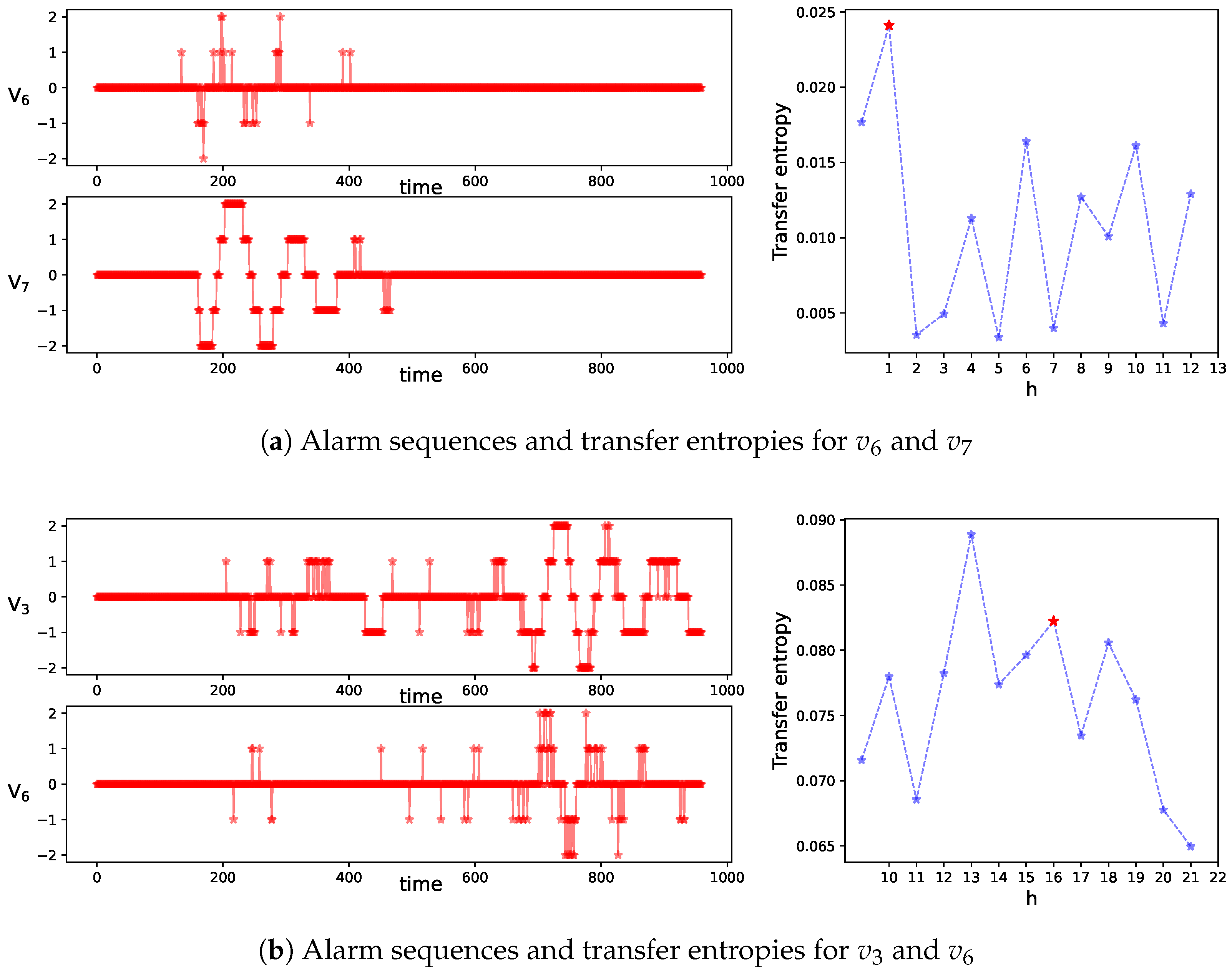
As illustrated in Figure 6, two variable pairs are used for demonstration. According to Equation (3), the estimated time delays between sequences are indicated by red stars in the figure. The prediction horizon h for each pair is closely related to the observed delay in the alarm sequences. In Figure 6a, the selected h for which the maximum transfer entropy occurs aligns well with the estimated delay. In contrast, Figure 6b shows a slight deviation between the two. In real-world sampled sequences, inherent fluctuations may prevent transfer entropy from peaking exactly at the true delay point. Instead, it typically maintains relatively high values across a range of delays.

It is important to emphasize that the maximum transfer entropy is not necessarily optimal for causal inference, as it may amplify spurious relationships without discrimination. In Section 5.3, we further demonstrate this amplification effect and evaluate the effectiveness of delay estimation through comparative analysis with other methods.

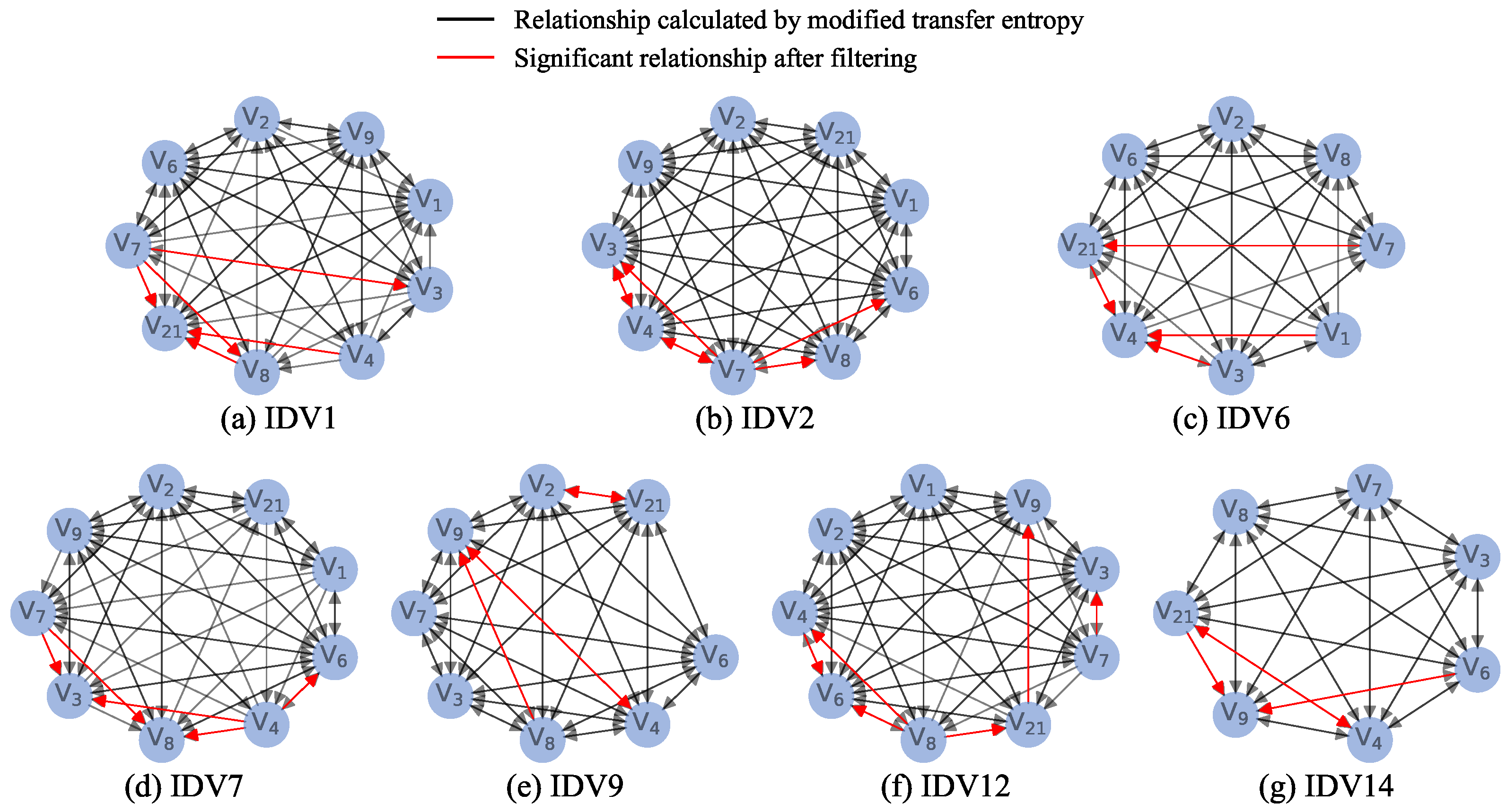
According to Equation (4), transfer entropies are computed for each variable pair. During the construction of the information transfer graph, all transfer entropies greater than or equal to zero are retained as edges. As shown in Figure 7, subgraphs for each disturbance scenario are generated following the steps outlined in Algorithm 1. Since each disturbance affects different variables and processes, the resulting subgraphs vary in structure. For example, in contrast to the IDV1 scenario—where the disturbance is a feed flow—the IDV14 scenario involves a water valve disturbance with a smaller impact. Consequently, the information transfer graph of IDV14 contains fewer relationships than that of IDV1.

4.5. Causal Graph Generation

Although the information transfer graph reveals the relationships of the variables in detail, the redundant edges are detrimental to understanding relationships. Following the steps of Algorithm 2, the relationships satisfying Equation (5) for each information transfer graph are filtered out and shown as the red line in Figure 7. Additionally, in this step, the cycles between pairs of variables are also removed to ensure the unidirectionality of causality.

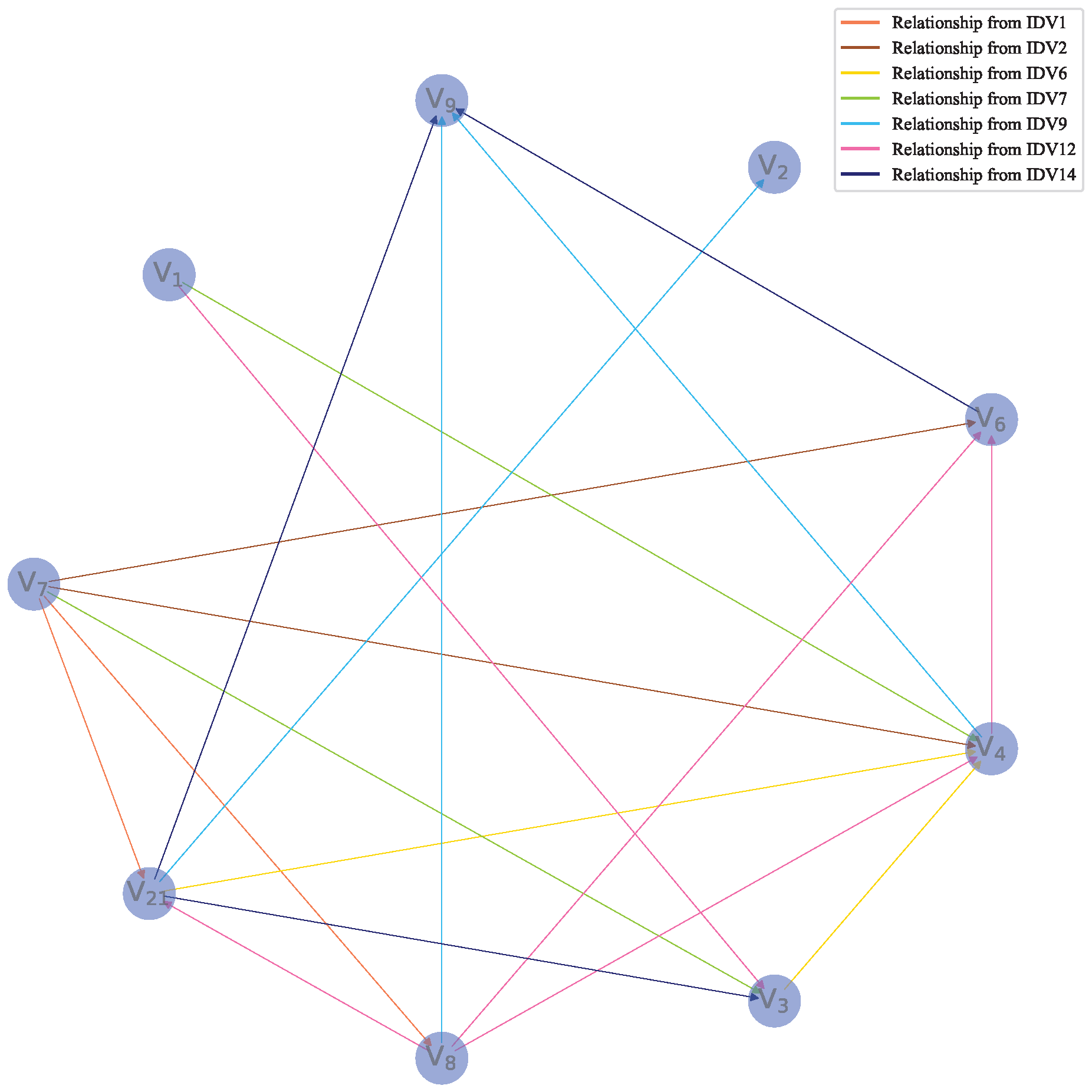
Based on the maximum rule mentioned in Section 3.4, the subgraphs of each dataset consisting of significant relationships are fused together, as shown in Figure 8. It should be noted that, although the redundant edges and the cycles are removed in Figure 8, there are multiple paths through which a variable can affect another. Hence, the graph after removing redundant relationships is reconstructed as a causal graph according to Algorithm 3, as shown in Figure 9. The relationships in Figure 9 show how the variables of the reactor subsystem in the TE process are affected.

5. Comparison and Discussion

To discuss the rationality of the experimental result, we analyze the process by which disturbances affect the variables in this section. In addition, some methods are compared with ours to illustrate the effectiveness of the improvements.

5.1. Analysis of Variable Relationships

Analyzing the TE process is crucial to understanding how variables affect each other when a disturbance is imposed. There are four feeds, A, C, D, and E, and one catalyst, B, in the TE process. According to Equation (7) and Figure 4, feeds A, C, D, and E undergo an exothermic reaction in the presence of catalyst B to produce products G, H, and F, which are subsequently transported to the condenser.

As the feed volume is the manipulated variable controlling the initial reaction phase, its measured value is naturally expected to be the first dependent variable. As listed in Table 2, the variable $v_4$ represents the A and C feed, so the trend of $v_4$ is affected by $v_1$, which concerns the A feed.

Since all reactions occur in the reactor, where a monitoring variable $v_6$ tracks the total feed amount, all variables related to the feed affect $v_6$. Because $v_2$ and $v_3$ are not involved in the compound feed measurement, they have a direct effect on $v_6$ as $v_4$.

When it comes to the reactor, the TE process sets up several variables to indicate the states of the reactor to monitor how the reaction is progressing. The feedback value of $v_8$, as a reflection of the overall state of the reactor, influences the control over the amount of feed. When the reactor level is abnormal, the control process will adjust the feed volume to offset the disturbance. Subsequently, with the entry of feeds, the exothermic reaction acts on the reactor, causing it to rise in temperature and pressure.

Moreover, with the reaction progressing, the cooling water is pumped in to cool the reactor so as to prevent an unrestricted increase in temperature. Thus, in addition to the exothermic reaction itself affecting the reactor temperature, the temperature of the cooling water can also impact it.

5.2. Evaluation Metrics

To evaluate the performance of causal relationship identification methods, we adopt three widely used metrics: Precision (Pre), Recall (Rec), and F1-score (F1). The definitions of these metrics are given as follows:

• Precision: The proportion of correctly identified true causal relationships among all predicted causal relationships. It reflects the accuracy of the identified results.

  $$\mathrm{Precision}={\displaystyle \frac{\mathrm{TP}}{\mathrm{TP}+\mathrm{FP}}}$$

  (9)
• Recall: The proportion of correctly identified true causal relationships among all actual causal relationships. It measures the method’s ability to cover true causal relationships.

  $$\mathrm{Recall}={\displaystyle \frac{\mathrm{TP}}{\mathrm{TP}+\mathrm{FN}}}$$

  (10)
• F1-score: The harmonic mean of Precision and Recall, providing a balanced measure of overall performance.

  $$\mathrm{F}1=2·{\displaystyle \frac{\mathrm{Precision}·\mathrm{Recall}}{\mathrm{Precision}+\mathrm{Recall}}}$$

  (11)

In the above formulas, TP denotes the number of true causal relationships correctly identified, FP represents the number of false positives (incorrectly identified relationships), and FN refers to false negatives (missed true relationships).

5.3. Results Comparison and Discussion

In this section, we design several comparative experiments to evaluate the effectiveness of the proposed method from the following perspectives: (1) How accurate are the causal relationships identified by our approach? (2) Does the proposed module enhance the accuracy of causal inference? (3) How can the proposed method be applied to alleviate industrial alarm overload, and is it effective in practice? The three subsections below address these questions through detailed comparisons and discussions.

5.3.1. Comparison of Causality Identification Results

Based on the analysis of how the variables are affected by the disturbance in the previous section and the results in [19,33], all necessary and obvious causal relationships are listed in

Table 4. Causality relationships comparison.

	[22]	[6]	[17]	[14]	Our Method
$v_1\to v_4$	Identified	Multi-step	Multi-step	Not identified	Identified
$v_3\to v_6$	Reversed	Not identified	Not identified	Identified	Multi-step
$v_4\to v_6$	Reversed	Not identified	Not identified	Identified	Identified
$v_8\to v_6$	Identified	Not identified	Identified	Identified	Identified
$v_6\to v_7$	Identified	Not identified	Not identified	Reversed	Reversed
$v_6\to v_9$	Not identified	Not identified	Not identified	Reversed	Identified
$v_{21}\to v_9$	Reversed	Reversed	Reversed	Identified	Identified
$v_2\to v_6$	Reversed	Not identified	Not identified	Not identified	Not identified

.

Analyzing Table 4 in conjunction with Figure 9, we can see that our method correctly identifies most of the relationships. However, although the relationship $v_3\to v_6$ can be identified in our method, it takes two steps. According to Figure 8, we note that $v_3\to v_4$ are significant relationships extracted from IDV6, which is a special disturbance. IDV6 differs from other small-amplitude-step disturbances in that it directly cuts off the A feed to make a serious fault. The cut-off of the A feed results in anomalies for the overall feed detection variables, causing the control process to begin adjusting other feed quantities to fit the change in A. Thus, the amount of feed as reactant E, which is involved in the same reaction, is significantly reduced.

For similar reasons, the relationship $v_7\to v_4$ was extracted from IDV2. Referring to Table 3, catalyst B is set up with a small step. Although it is claimed that the ratio of A and C feeds remain constant, the step in B causes a sudden increase in reactor pressure, which affects the amount of feed.

A comparison between the TE process and the causal structure inferred from disturbance data reveals the presence of a feedback mechanism. Because the disturbances occur during the ongoing reaction rather than at its initial stage, the identification of certain causal directions may be influenced by this dynamic feedback behavior.

To further demonstrate the effectiveness of our proposed approach, we conducted comparative experiments with both entropy-based [6,14,17] and non-entropy-based [22] causal inference methods. The evaluation results are shown in Figure 10 and

Table 5. Performance comparison table of different methods.

	[22]	[17]	[14]	Ours
Precision	0.11	0.13	0.57	0.71
Recall	0.38	0.13	0.50	0.62
F1-score	0.17	0.13	0.53	0.67

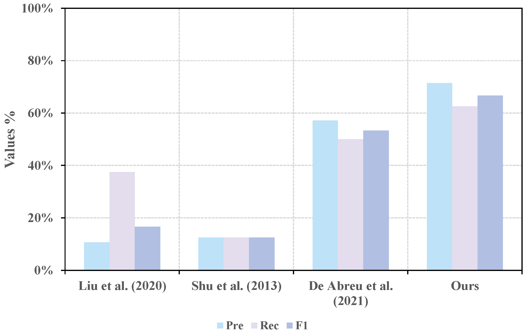
(the bold black font in the table indicates the best results), and the specific causal relationships identified by each method are listed in Table 4. For fairness, only the causal inference components of each baseline method were implemented. The number of correct relationships identified by the five methods within one or two steps are 3, 1, 2, 4, and 6, respectively. Our proposed method achieved the highest scores in all three evaluation metrics: Precision, Recall, and F1-score.

The methods in [6,17] attempt to improve transfer entropy computation by increasing the prediction horizon and reducing the temporal gap between the current point and the predicted point. However, they ignore the dynamic variability in the optimal prediction horizon. As a result, sequence responses may become misaligned under abnormal operating conditions, leading to incorrect causal mappings and degraded inference accuracy.

Building upon [6], De Abreu et al. [14] introduced a dynamic search strategy to determine the optimal h value (ranging from 1 to 50) that maximizes transfer entropy. Although this approach can strengthen genuine causal links, it also amplifies spurious ones. Consequently, during the filtering of significant relationships, true causal links may be overshadowed by false ones.

Compared to our method, the results of [14] missed two key relationships: $v_1\to v_4$ and $v_6\to v_9$. As shown in Figure 9, the transfer entropy values on these edges are relatively low compared to others, making them more susceptible to removal under the dynamic h selection strategy. This observation validates our theoretical analysis and is also reflected in the quantitative metrics: our method outperforms the dynamic h strategy in all metrics by approximately 13% on average.

We also compared our method with a non-entropy-based approach [22]. As shown in Table 4 and Figure 10, this method managed to capture a relatively high number of true causal relationships, resulting in a favorable Recall. However, unlike transfer entropy-based methods, it tends to retain a larger number of causal links overall, thereby reducing its Precision and leading to a lower F1-score.

It is worth noting that all true causal relationships were successfully identified by our method, except for $v_2\to v_6$. The failure to detect this link is due to the fact that the only disturbance affecting unit B is an abnormal temperature, while no variable was configured to monitor B temperature directly. As a result, the abnormal temperature in B does not induce observable fluctuations in $v_2$ (the feed B), rendering this causal relationship undetectable in practice.

5.3.2. Comparison of Different Delay Calculation Methods

To highlight the effectiveness of CCF in the proposed framework, a comparative analysis was conducted against two widely used delay estimation techniques: the mutual information-based method [34] and the dynamic time warping-based method [35]. In this comparison, only the delay estimation module was replaced, while all other components of the framework remained unchanged. The experimental results, presented in Figure 11 and

Table 6. Performance comparison table of different delay calculation methods.

	[34]	[35]	Ours
Precision	0.17	0.29	0.71
Recall	0.12	0.25	0.62
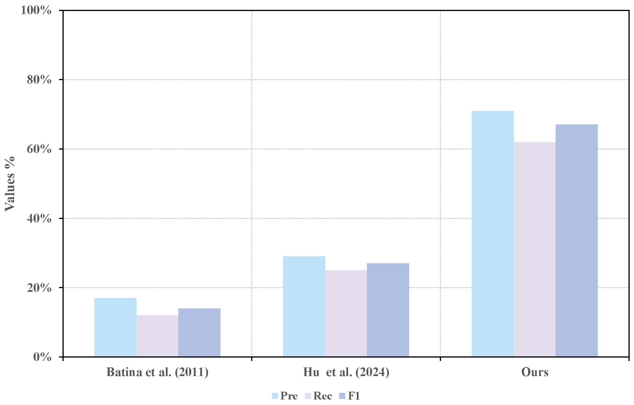
F1-score	0.14	0.27	0.67

, demonstrate that our method achieves superior performance across all evaluation metrics. Notably, the F1-score exceeds that of the two alternative methods by 53% and 40%, respectively. In addition, our method successfully identifies four more correct relationships than the approach reported in [34] and three more than the approach in [35]. These findings confirm the strong adaptability of CCF to the proposed framework and its significant contribution to improving the overall accuracy of causal analysis.

5.3.3. Effectiveness of Multi-Valued Alarm Processing

In this section, we evaluate the effectiveness of the proposed multi-valued alarm processing module. Specifically, during the data preprocessing stage, we apply both a five-level and a three-level alarm strategy to the sampled sequences, followed by causal relationship identification. As illustrated in Figure 12 and

Table 7. Performance comparison table of different alarm processing strategies.

	5-Level	3-Level
Precision	0.71	0.29
Recall	0.62	0.25
F1-score	0.67	0.27

, the overall identification performance achieved by the five-level alarm strategy significantly outperforms that of the three-level strategy. In particular, its Precision, Recall, and F1-score are 42%, 37%, and 40% higher than the three-level strategy, respectively. This demonstrates that the five-level alarm strategy is more capable of capturing subtle variations in sequence trends and distinguishing causal relationships of different intensities, thereby enabling more precise causality identification.

5.3.4. Effectiveness of Sequence Dynamic Alignment

In order to further demonstrate the effectiveness of our optimized transfer entropy method, a large-scale calculation of transfer entropy values, spanning multiple typical scenarios, is presented in Figure 13. Through a comprehensive review of the pertinent literature, two typical strategies are selected for comparison with our approach: the fixed ‘h’ [6,10,16] and the ‘h’ chosen to maximize the transfer entropy [11,12,13,14,17,18]. As shown in Figure 13, the first column corresponds to a fixed prediction horizon, while the subsequent two columns represent dynamic prediction horizons, with the last column showing the results obtained using our method.

In Figure 13, deeper colors indicate stronger causal relationships. A holistic comparison of the three matrix columns clearly demonstrates that our method effectively reduces the values of insignificant relationships, thereby highlighting significant relationships. The boundary between insignificant and significant relationships is also more sharply delineated. As expected, compared to a fixed prediction horizon, the maximum value strategy indiscriminately amplifies various relationships, regardless of their significance.

In IDV1, our method effectively reduces the transfer entropy for the erroneous relationships $v_7\to v_3$ and $v_4\to v_{21}$. This reduction in entropy values is similarly evident in IDV7 for $v_1\to v_3$ and $v_4\to v_{21}$, as well as in IDV12 for $v_7\to v_3$ and $v_4\to v_{21}$. For instance, considering the relationship $v_4\to v_{21}$, which is incorrectly identified by both methods in all three scenarios, it exhibits a considerable degree of ambiguity. In IDV7 and IDV12, our method almost entirely eradicates the causal relationship between $v_4$ and $v_{21}$. While a causal relationship is identified in IDV1, its entropy value is notably decreased in comparison to the fixed prediction horizon strategy.

Our method not only effectively weakens erroneous relationships, but also amplifies the correct causal relationships. In IDV12, the entropy values for $v_4\to v_6$, $v_8\to v_6$, and $v_{21}\to v_9$ are increased in contrast to the other two approaches, thus underscoring the importance of the valid relationships across the entire matrix. In IDV7, the entropy value of $v_1\to v_4$ rises compared to the fixed prediction horizon strategy, although it remains lower than the maximum transfer entropy strategy. However, the maximum transfer entropy strategy amplifies other relationships, causing $v_1\to v_4$ to be inconspicuous in the matrix, even ranking lower than erroneous relationships such as $v_7\to v_8$, $v_4\to v_8$, and $v_1\to v_8$. This could potentially result in its exclusion during the significance filtering stage. In contrast, our method simultaneously strengthens correct relationships and reduces the entropy values of erroneous relationships. This enables even a slight enhancement to ensure their retention as significant relationships in subsequent experiments.

5.3.5. Effectiveness of Alarm Mitigation

The resulting causal graph reveals the underlying causal relationships among variables. In other words, it provides insight into the temporal sequence of sensor responses to disturbances and the subsequent propagation of their effects across variables. This is particularly critical in ICS analysis, where inexperienced operators may struggle to promptly identify the causes and effects of alarms when facing a large number of alarms. Over time, operators may fail to recognize the downstream variables affected by disturbances and thus be unable to take appropriate mitigation measures, ultimately leading to inefficient alarm handling. Prolonged inaction on alarms may even disrupt the normal operation of the entire process system.

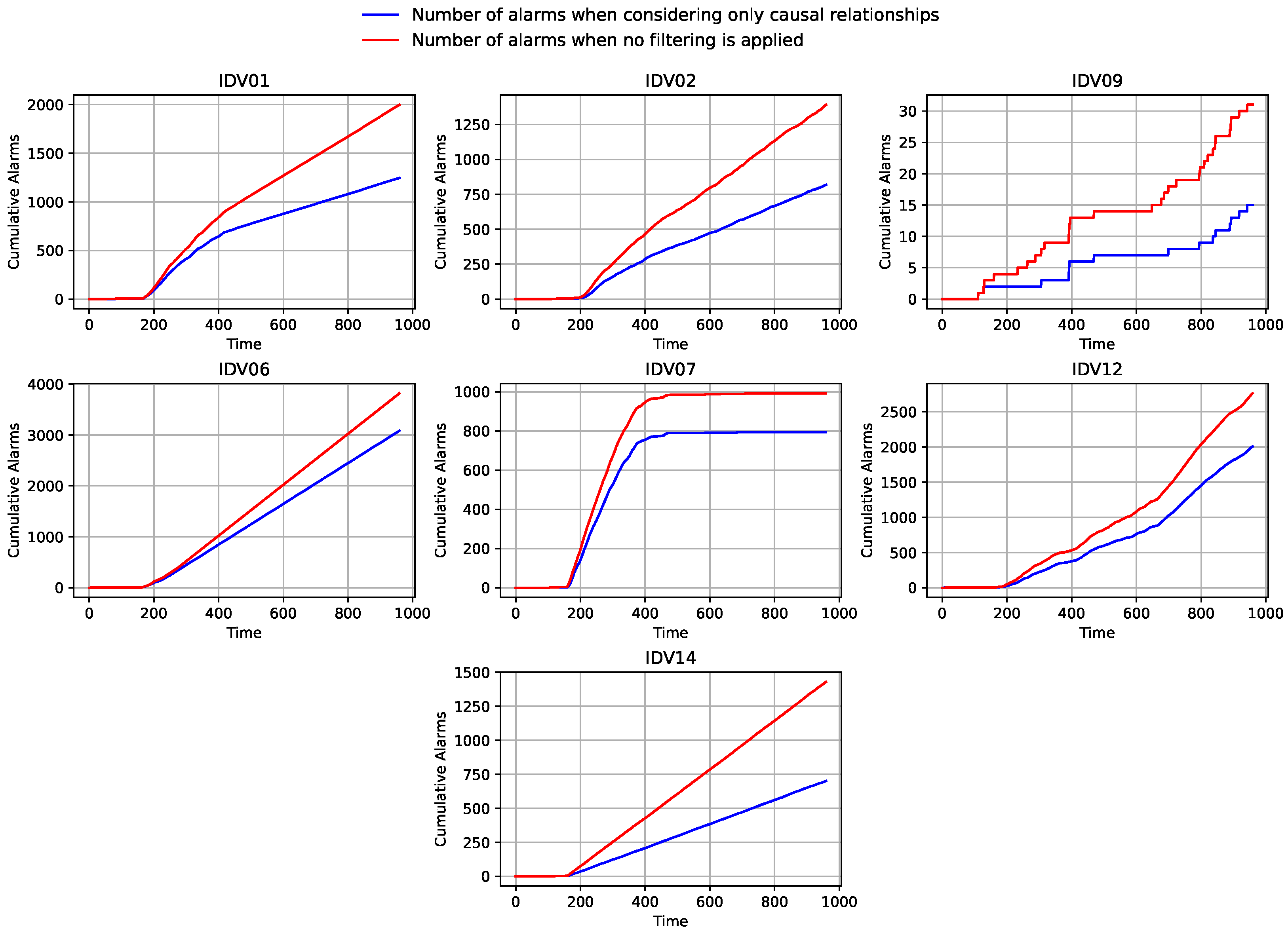
To illustrate the significant role of the proposed method in assisting system operators in handling alarm overload, we conducted experiments in seven anomaly scenarios. In these tests, we simulated how system operators use the causal graph in practice. Once a disturbance occurs, operators focus only on variables that show direct causal relationships to the current anomalies, while ignoring unrelated secondary variables. This process effectively guides operator attention and ensures that limited cognitive resources are concentrated on the most critical variables.

As shown in Figure 14, we tested alarm reduction on datasets of different scales. Although the percentage of reduction varied, the effectiveness of alarm reduction was consistently significant regardless of alarm amount. Throughout the experiments, we observed that specific reduction proportions were influenced partly by the physical topology of the system. The reduction was more pronounced in sensor-sparse areas, which is reasonable, as causal relationships in sensor-dense regions are more complex and naturally result in a decrease in alarm reduction. However, our method is not limited by data scale. For example, both IDV9 and IDV14 represent systems of different sizes, yet each achieved an alarm reduction exceeding 50%. This result demonstrates that the causal graph can eliminate more than half of the secondary alarms, substantially reducing operator workload and improving the efficiency of alarm management.

According to the comparison and discussion above, it is clear that the method proposed in this paper is generally better at identifying the causal relationships between industrial alarm data and plays an important role in the alarm management phase.

5.3.6. Parameter Analysis

In this section, a sensitivity analysis is conducted on two groups of parameters, namely, the historical sequence lengths, k and l, and the confidence level of the threshold.

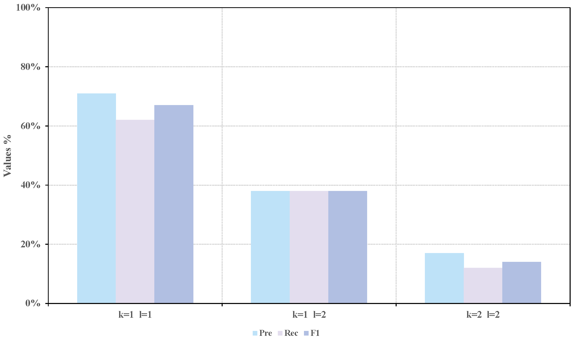
As illustrated in Figure 15 and

Table 8. Sensitivity analysis of historical sequence lengths k and l.

	$\mathit{k}=1,\mathit{l}=1$	$\mathit{k}=1,\mathit{l}=2$	$\mathit{k}=2,\mathit{l}=2$
Precision	0.71	0.38	0.17
Recall	0.62	0.38	0.12
F1-score	0.67	0.38	0.14

, three settings of historical sequence lengths were tested. The results indicate that causal identification achieves the best performance when $k=1$ and $l=1$, yielding an F1-score that is 29% and 53% higher than those obtained under $k=1, l=2$, and $k=2, l=2$, respectively. As the sequence length increases, performance gradually declines, suggesting that the method is sensitive to the choice of historical length. This phenomenon can be explained by the fact that the five-level alarm sequences already contain inherent trend information, which positively influences short-sequence modeling. With longer sequences, additional noisy fluctuations may be introduced, which can distort the transfer entropy calculation and consequently reduce the effectiveness of the method.

Figure 16 and

Table 9. Sensitivity analysis of confidence level.

	Confidence Level = 95%	Confidence Level = 90%	Confidence Level = 80%
Precision	0.50	0.71	0.43
Recall	0.38	0.62	0.38
F1-score	0.43	0.67	0.40

further present the results obtained under three different confidence levels. The F1-score reaches its maximum (67%) when the confidence level is set to 90%. Under the other two settings, only about half of the true relationships can be identified, with F1-scores of 43% and 40%, respectively. Excessively high confidence levels severely restrict the number of selected causal pairs, lowering accuracy. Conversely, overly low confidence levels may detect more relationships, but can introduce false links. The model shows weaker sensitivity to the confidence level than to the sequence length parameter. Due to the multi-subgraph fusion strategy, which facilitates precise identification across disparate confidence levels.

Considering the composite metrics, this study adopts the configuration parameters $k=1$, $l=1$, and a 90% confidence level as the optimal parameter settings.

5.3.7. Runtime for Different System Scales

As illustrated in Figure 17 and

Table 10. Runtime for different system scales.

Node Numbers	Time (s)
10	1.88
50	18.40
100	70.59
150	153.12
200	266.85
250	422.27
300	608.79
350	821.50
400	1064.07
450	1350.47
500	1662.93

, we conducted experiments on systems with node sizes ranging from 10 to 500. It can be observed that when the system contains approximately 200 nodes, the runtime can be kept within 5 min—roughly equivalent to one sampling interval—which is considered acceptable in practical applications. However, as the number of nodes increases further, the runtime grows in a power-law manner with respect to the total number of nodes. Based on these results, we recommend applying the proposed method to small- and medium-scale industrial control systems with no more than 200 nodes.

6. Conclusions

In this paper, the modified transfer entropy method optimized by the time delay estimation is proposed to infer the causal relationships between industrial alarms, and solves the problem of overloading alarms due to disturbances that exceed the management capacity of operators. The introduction of the time delay estimation avoids the false causality induced by misaligned alarm sequences and contributes to highlighting critical causal links. In addition, a multi-scale subgraph-fusion strategy is designed to overcome the degradation of causal strength at the disturbance boundaries. The method proposed in this paper is validated in the well-known Tennessee Eastman process. And the experimental results show that our method can effectively increase the gap between true and false causal relationships, highlight weakened relationships, and efficiently identify true causal relationships. Compared to the existing methods, the causal graph obtained in this paper demonstrate greater consistency with the result of the variable propagation analysis, achieving a higher identification rate of key relationships. The inferred causal structure can guide operators in alarm management, enabling the suppression of over 50% of redundant alarms and thereby substantially improving response efficiency. In a scenario with M disturbances, N sensors, and sequence length T, the computational complexities of the modified transfer entropy module, the multi-scale importance filtering module, and the subgraph fusion module are $\mathcal{O}(M·N^2·T)$, $\mathcal{O}(M·N^{2}logN)$, and $\mathcal{O}(M·N^2)$, respectively. Therefore, the overall computational complexity of the proposed method is $\mathcal{O}(M·N^2·T)$. To ensure real-time applicability, we recommend deploying this method in industrial systems with no more than 200 nodes or adopting a distributed implementation for larger-scale systems.

Despite its promising performance, the proposed method also has certain limitations. The results can be sensitive to the discretization granularity used in transforming continuous measurements into multi-valued alarm sequences. Moreover, noisy measurements and overlapping latency effects among multiple variables may introduce uncertainty into the causal inference process. These factors should be considered when applying the method to large-scale industrial environments.

This study also highlights broader research directions, particularly in uncovering multivariate interaction patterns. The proposed approach can be integrated with sequence prediction models in machine learning to enable dynamic causal relationship identification, thereby broadening its application scope. Moreover, future work will focus on improving computational efficiency to facilitate the deployment of the method in industrial scenarios across diverse domains.