A Traffic Forecasting Framework for Cellular Networks Based on a Dynamic Component Management Mechanism

Abstract

Accurate forecasting of cellular traffic in non-stationary environments remains a formidable challenge, as real-world traffic patterns dynamically evolve, emerge, and vanish over time. To tackle this, we propose a novel meta-learning framework, GMM-SCM-DCM, which features a Dynamic Component Management (DCM) mechanism. This framework employs a Gaussian Mixture Model (GMM) for probabilistic meta-feature representation. The core innovation, the DCM mechanism, enables online structural evolution of the meta-learner by dynamically splitting, merging, or pruning Gaussian components based on a bimodal similarity metric, ensuring sustained alignment with shifting data distributions. A Single-Component Mechanism (SCM) is utilized for precise base learner initialisation. To ensure a rigorous and realistic validation, we reconstructed the Telecom Italia Milan dataset by applying unsupervised clustering and meta-feature engineering to identify and label four distinct functional zones: residential, commercial, mixed use, and crucially, non-stationary areas. This curated dataset provides a critical testbed for non-stationary forecasting. Comprehensive experiments demonstrate that our model significantly outperforms traditional methods and meta-learning baselines, achieving a 9.3% reduction in MAE and approximately 70% faster convergence. The model’s superiority is further confirmed through extensive ablation studies, robustness tests across base learners and data scales, and successful cross-dataset validation on the Shanghai Telecom dataset, showcasing its exceptional generalization capability and practical utility for real-world network management.

1. Introduction

With the rapid advancement of fifth-generation mobile communications technology (5G) and Internet of Things (IoT), mobile network traffic demonstrates explosive growth and high dynamism. 5G and its evolving technology, B5G (Beyond 5G) networks, have introduced three typical application scenarios: enhanced Mobile Broadband (eMBB), massive Machine-Type Communications (mMTCs), and Ultra-Reliable Low-Latency Communications (URLLCs). These scenarios pose new challenges for traffic prediction. The eMBB scenario, characterized by high-speed data transmission, exhibits bursty traffic patterns and high bandwidth demands, with the primary prediction target being throughput. The mMTC scenario, characterized by massive device connectivity, shifts the prediction focus from throughput to the number of connections. The URLLC scenario requires extremely low latency and high reliability, necessitating the prediction of network load to ensure quality of service. Typical applications of these scenarios include smart cities, connected vehicles, and the industrial Internet. Accurate traffic prediction not only enhances user experience but also significantly reduces operational costs, improving the autonomy and intelligence of networks.

Traditional traffic prediction methods are mostly based on statistical models or shallow machine learning approaches. The Seasonal Autoregressive Integrated Moving Average (SARIMA) model has long been used for communication traffic prediction due to its effective characterization of seasonality and trend components [1]. Support Vector Regression (SVR), on the other hand, handles nonlinear relationships through kernel functions and has demonstrated advantages in early traffic prediction [2]. Although these methods perform well in stationary time series prediction, their assumptions of linear or static modeling make it difficult to capture the non-stationarity and multimodal evolution characteristics caused by mixed services, user mobility, and sudden events in 5G environments [3]. In recent years, deep learning models such as Long Short-Term Memory (LSTM) and Gated Recurrent Unit (GRU) have been widely applied to traffic prediction tasks due to their powerful sequence modeling capabilities [4,5]. However, these methods typically rely on large amounts of labeled data for training and exhibit limited generalization capability when faced with data distribution shifts or unseen traffic patterns, often leading to performance degradation [6]. This makes it challenging for them to adapt to the dynamic and variable environment of 5G networks.

Meta-learning, as a “learning to learn” paradigm, enables models to quickly adapt to new tasks by extracting shared knowledge from multiple related tasks, making it particularly suitable for addressing model initialisation problems in few-shot scenarios [7]. In the field of traffic prediction, meta-learning constructs abstract representations of task distributions to provide personalized model initialisation strategies for different base stations or regions, thereby significantly improving prediction efficiency and accuracy. However, most existing meta-learning traffic prediction models are based on the assumption of stationary traffic patterns. Their meta-learners (such as K-Nearest Neighbors, deep neural networks, or Gaussian mixture models) often employ fixed structures or a fixed number of components, making it difficult to effectively handle concept drift issues caused by factors like changes in base station functionality or the introduction of new services in real-world networks.

The core challenge of non-stationary traffic patterns lies in their underlying data distributions, which are not static but undergo structural shifts over time, space, and external events (such as holidays, emergencies, or cyberattacks). These manifest as: (1) the emergence of new patterns (e.g., newly built metro stations or schools); (2) the disappearance of old patterns (e.g., decommissioned factories); (3) the merging and splitting of patterns (e.g., evolution of mixed commercial–residential zones); and (4) the ambiguity of pattern boundaries (e.g., functionally mixed areas). These changes cause meta-learning models based on fixed component numbers (e.g., GMM with fixed K values) to suffer from pattern omission, component degradation, and inefficient resource allocation, severely limiting their applicability and scalability in real-world networks.

To address these challenges, this paper proposes a meta-learning traffic forecasting model based on a Dynamic Component Management (DCM) mechanism, termed GMM-SCM-DCM. Building upon the Gaussian Mixture Model (GMM) as its meta-learning backbone, the model introduces dynamic component splitting and merging mechanisms to achieve adaptive tracking and modeling of non-stationary traffic patterns. Specifically, a bimodal similarity metric combining probabilistic and spatial similarity is designed to evaluate pattern novelty in new tasks, thereby triggering component generation, merging, or removal operations. Furthermore, a Single-Component Mechanism (SCM) is employed as the initial weight allocation strategy for the base learner, mitigating pattern confusion and training instability potentially caused by multi-component synthesis.

The major contributions of this paper include:

• Proposing a meta-learning framework with a DCM mechanism, enabling the model to perform online identification, adaptation, and evolution of 5G traffic patterns.
• Designing a dual-modal similarity metric and a three-layer response strategy to achieve fine-grained initialisation and rapid adaptation for different service modes (such as eMBB and mMTC).
• Constructing a non-stationary traffic evaluation benchmark incorporating typical 5G service modes based on a real cellular dataset, and systematically validating the model’s advantages in prediction accuracy, convergence speed, and generalization capability.

The paper is structured as follows. Section 2 systematically reviews 5G/B5G requirements and existing traffic prediction approaches. Section 3 details the GMM-SCM-DCM architecture and algorithms. Section 4 describes the experimental setup and datasets. Section 5 presents and discusses the results. Finally, Section 6 concludes the paper and suggests future research directions.

2. Related Work

Current mobile communication networks (5G and B5G) face challenges posed by the exponential growth in users and devices, with massive data traffic exerting significant pressure on finite network resources. In response, Aouedi et al. note that precise analysis and forecasting of network traffic form the foundation for developing intelligent networks and optimizing service design and management [8]. Research by Mohan et al. similarly demonstrates that cellular traffic forecasting models enable operators to better adapt to network demand, optimize resource utilization, and thereby enhance user experience. Consequently, precise traffic prediction is not merely an “option” for network optimization but an “essential” for achieving proactive, intelligent network management, providing core data support for critical functions such as dynamic resource allocation, base station energy conservation, and load balancing [9].

To contextualize our work, this chapter reviews cellular traffic prediction with respect to both application needs and technical evolution. Section 2.1 analyzes the new challenges posed by 5G/B5G scenarios. Section 2.2 then traces the evolution of prediction methods, from statistical models to deep learning and emerging paradigms like meta-learning. This review shows that our dynamic meta-learning framework addresses the growing demands of non-stationary 5G/B5G environments.

2.1. Traffic Prediction in 5G/B5G Networks: Applications and Challenges

The core vision of the fifth-generation mobile communication and its evolving technologies (5G/B5G) is to build an intelligent, interconnected society. Its three typical application scenarios—Enhanced Mobile Broadband (eMBB), massive Machine-Type Communications (mMTCs), and Ultra-Reliable Low-Latency Communications (URLLCs)—fundamentally reshape the nature of cellular network traffic [10]. This transformation upgrades accurate traffic prediction from an “optimization method” to a “necessity” for the network to fulfill its core promises.

At the application level, traffic prediction is a key enabling technology for 5G/B5G to achieve efficient and intelligent operations. Firstly, in dynamic resource allocation, the network needs to perform flexible spectrum and power scheduling in the time, frequency, and spatial domains in advance based on the predicted future load to avoid network congestion during eMBB traffic peaks while ensuring resource reservation for URLLC services. Secondly, predictive capability is crucial for network slicing. Operators need to accurately estimate the medium- to long-term traffic demands of different slices (e.g., an 8K video stream slice and a massive IoT slice) to achieve efficient slice lifecycle management and SLA assurance [11]. Furthermore, energy efficiency optimization (such as base station sleep modes) heavily relies on reliable short-term prediction. During low-load periods like midnight, incorrectly waking up a base station or incorrectly shutting one down can lead to energy waste or service interruptions. Additionally, prediction technology is widely used in scenarios such as load balancing, cache strategy optimization, and edge computing task offloading [12].

However, the inherent characteristics of 5G/B5G traffic also pose unprecedented challenges for prediction models. The core challenge stems from the intrinsic non-stationarity of the traffic. This is mainly reflected in three aspects: The first is service heterogeneity. eMBB services (like 4K/8K video) generate high-throughput, bursty “elephant flows”; mMTC services (like smart meter reading) manifest as massive connections with small data packets—“mice flows”—where the number of connections, not the data volume, is the key metric; URLLC services (like industrial control) are extremely sensitive to delay and jitter, making their traffic patterns difficult to capture with traditional models [13]. These vastly different traffic streams randomly superimpose in time and space, causing the statistical properties (like mean, variance) of the aggregate traffic sequence to no longer be constant. The second aspect is spatio-temporal dynamics. Spatially, the evolution of urban functional areas (e.g., construction of new commercial districts, relocation of old industrial zones) leads to structural changes in the traffic patterns of a base station’s service area [14]. Temporally, unexpected social events (e.g., major sporting events) or the popularity of new applications (like the Metaverse, AIGC) can instantly break inherent traffic periodic patterns, generating “new modes” not present in the training data. The third is resource virtualization. The introduction of network slicing and edge computing means traffic is no longer solely tied to physical locations but is associated with logical slices and virtualized functions, which increases the complexity of traffic traceability and modeling [11].

Traditional prediction models (e.g., SARIMA) and many static deep learning models are based on the fundamental assumption that the data generation process is stationary or slowly changing. Consequently, they struggle to effectively handle the severe and persistent concept drift problem in the aforementioned 5G/B5G environment. They often perform well initially after deployment, but as the network environment and service composition evolve, their prediction performance degrades rapidly.

As shown in

Table 1. Applications, challenges, and model requirements for 5G/B5G traffic prediction.

Application Domain	Specific Requirements and Prediction Targets	Core Challenges	Requirements for Prediction Models
Dynamic Resource Allocation	Short-term prediction (minute to hour level) of base station/cell-level throughput for dynamic spectrum and power adjustment.	Bursty eMBB traffic causes sharp peaks; multiple services compete for the same resource pool.	High-precision short-term prediction capability; rapid response to bursty traffic.
Network Slicing Management	Medium- to long-term prediction (hour to day level) of traffic demand and connection count per network slice for pre-configuring slice resources.	Vastly different and independently changing traffic patterns across slices (eMBB, mMTC, URLLC).	Multi-variable prediction capability; ability to distinguish and independently model different service patterns.
Energy Efficiency Optimization and Base Station Sleep	Ultra-short-term prediction (15 min to 1 h) of cell-level load to decide base station (or carrier) sleep/wake cycles.	High prediction uncertainty: incorrect sleep causes service interruption, and incorrect wake-ups waste energy.	High reliability; strong adaptation to diurnal patterns; good uncertainty calibration.
Load Balancing	Short-term prediction of neighboring cell load differences to execute handovers or traffic steering.	User mobility causes spatial “hotspots” to shift rapidly.	Strong spatial correlation modeling capability; fast online inference.
mMTC Random Access Control	Predicting connection request count to optimize preamble allocation and access strategy.	Massive devices may trigger access simultaneously, making the prediction target fundamentally different from traditional throughput.	Ability to predict non-throughput KPIs like “connection count”; capability to handle count data.
URLLC Resource Reservation	Predicting the occurrence probability and resource demand of ultra-low latency services.	URLLC traffic events are sparse but require extremely high reliability; signals are weak in traditional time series data.	Sensitivity to rare event detection; support for very low-latency inference pipelines.

, 5G/B5G networks not only expand the scope of requirements for traffic prediction but also, due to their inherent non-stationarity and heterogeneity, place higher demands on the adaptability, robustness, and evolvability of prediction models. An ideal prediction framework should possess a “lifelong learning” capability, enabling it to continuously track changes in network state, dynamically adjust its own structure to capture newly emerging traffic patterns, and forget obsolete ones. This positioning is precisely the starting point of the research work in this paper.

2.2. Evolutionary Path of Traffic Prediction Technology

2.2.1. Traditional Methods and Early Deep Learning Models

Early cellular traffic forecasting research primarily drew upon classical time series analysis methods. Tran et al.’s work demonstrated that exponential smoothing, owing to its low computational complexity and cost-effectiveness, was applied to short-term forecasting for voice and data services [15]. Subsequent research by Tran et al. further confirmed that, across various traffic scenarios, exponential smoothing outperformed more complex models such as multiplicative seasonal ARIMA [16]. However, Jaffry et al. [17] noted that statistical models such as ARIMA typically rely on linearity or stationarity assumptions, making it difficult to accurately capture the nonlinear dynamic characteristics prevalent in cellular traffic.

To overcome the limitations of traditional methods, researchers have turned to machine learning, particularly deep learning. A comparative study by Santos Escriche et al. [18] found that Feedforward Neural Networks (FFNNs) outperform statistical models for short-step length forecasts (e.g., 1-step and 10-step); however, for longer-term forecasts (20-step), statistical models such as autoregressive models demonstrate superior performance. As a potent tool for addressing time series problems, Long Short-Term Memory (LSTM) networks are widely employed due to their ability to effectively capture temporal correlations and nonlinear features within data. For instance, Cao and Liu [19] demonstrated that LSTM-based forecasting models significantly outperform stacked autoencoder networks in terms of accuracy. Concurrently, the work of Kurri et al. [20] validated LSTM’s capability to predict base station traffic effectively within novel blockchain-based mobile network architectures, thereby enabling more secure network connectivity and functional optimization. However, despite demonstrating commendable performance in stationary or short-term forecasting tasks, these approaches exhibit notable limitations when confronting the non-stationary traffic patterns prevalent in real-world cellular networks. Existing approaches predominantly rely on the strong assumption of fixed distributions in historical data, struggling to effectively handle the dynamic emergence, disappearance, or abrupt changes in traffic patterns caused by factors such as the evolution of urban functional zones or sudden public events. Particularly when test data distributions deviate significantly from training distributions, models like LSTMs are prone to substantial performance degradation, lacking the capacity for continuous adaptation to underlying data distribution drift.

2.2.2. Spatio-Temporal Fusion Based on Convolutional and Recurrent Networks

Cellular traffic exhibits both temporal periodicity and burstiness and strong spatial correlations, wherein neighboring base stations’ traffic patterns often influence one another. Consequently, modeling complex spatio-temporal dependencies has become central to modern traffic forecasting research. A mature paradigm involves combining Convolutional Neural Networks (CNNs) with Recurrent Neural Networks (RNNs) and their variants (e.g., LSTMs). The core concept leverages CNNs’ potent local feature extraction capabilities to capture spatial characteristics between base stations, followed by the use of RNNs to learn the temporal evolution of these features. For instance, Zhang et al. proposed a Hybrid Spatio-Temporal Network (HSTNet), which employs deformable convolutions to enhance spatial feature capture flexibility and incorporates temporal attributes as auxiliary information, achieving precise city-level cellular traffic forecasting [21]. Similarly, Zhan et al. employed a CNN-based model to forecast cell traffic when designing resource allocation schemes for software-defined ultra-dense visible light communication networks, thereby enabling the formulation of efficient resource scheduling strategies in advance [22]. Furthermore, research by Hu et al. demonstrated that preprocessing raw traffic data using a Butterworth filter before feeding it into a CNN–LSTM hybrid model can also effectively enhance prediction accuracy [23].

2.2.3. Applications of Graph Neural Networks in Spatial Modeling

Whilst CNN-based methods effectively handle regular grid-based data, the topology of cellular base stations inherently constitutes a non-Euclidean graph structure. Consequently, Graph Neural Networks (GNNs), capable of learning directly on graph-structured data, have been introduced to this domain and have rapidly emerged as predominant approaches for spatial modeling. Khalid et al. [24] proposed that GNN applications offer novel approaches to resolving base station congestion issues. By accurately forecasting future traffic peaks, aerial platforms such as drones can be pre-deployed to distribute traffic loads. To capture intricate spatial relationships with greater precision, researchers have designed various hybrid models. For instance, Chen et al. [25] proposed a Spatio-Temporal Parallel Prediction Model (STP-GLN), comprising a spatial module utilizing Graph Convolutional Networks to learn spatial features and a temporal module employing Long Short-Term Memory networks to learn temporal features, with the results from both modules being weighted and fused. Zhang et al.’s Hybrid Graph Convolutional Recurrent Network (HGCRN) combines static graph convolutions with metagraph learning to construct adjacency matrices that transcend geographical proximity, thereby enabling deeper insights into dynamic interactions within networks [26]. Cai et al.’s Dual-Branch Spatio-Temporal Graph Neural Network (DBSTGNN-Att) first constructs an attribute K-Nearest Neighbor Graph based on data feature similarity to fuse multimodal features, then concurrently extracts spatio-temporal information through a dual-branch architecture [27]. Furthermore, Lin et al. [28] applied a Multivariate Propagation Graph Attention Network to process outdoor cellular traffic data, serving predictive tasks in domains such as intelligent transportation.

2.2.4. Application of Attention Mechanisms and Transformer Architecture

Attention mechanisms enable models to dynamically assign weights to features across different spatio-temporal locations, thereby focusing on critical information. For instance, Xiao et al. [29] combined Diffusion Convolutional Gated Recurrent Units (DCGRUs) with multi-head attention to construct the DCG-MAM model, which effectively captures complex spatio-temporal dependencies, periodicity, and external influences. Ma and Yang [30] proposed an end-to-end framework based on deep state space models integrated with attention mechanisms, utilizing CNNs and attention to capture spatial dynamics while incorporating Kalman filtering for temporal modeling. Inspired by natural language processing, Transformer architectures have been introduced to traffic forecasting. A prime example is the TSENet model proposed by Wang et al., which incorporates dedicated temporal and spatial Transformer modules for extracting temporal features and integrating spatial information, respectively [31]. Tang et al. [32] took a novel approach, combining a frequency–domain multilayer perceptron with a Multi-Scale Attention Network to analyze and forecast traffic data from a frequency–domain perspective.

2.2.5. Decomposition and Multi-Dimensional Feature-Based Methods

Raw cellular traffic sequences typically embody multiple intertwined patterns, rendering a “divide and conquer” strategy effective. Gong et al.’s Knowledge Graph-Driven Decomposition Approach (KGDA) exemplifies this, decomposing traffic into a regular pattern determined by static environmental factors and dynamic residual fluctuations, each modeled separately [33]. Similarly, the DIC-ST framework proposed by Zhang et al. first decomposes complex time series into trend, periodic, and fundamental components, then employs causal structure learning to uncover causal relationships between different base stations across these components. Beyond decomposition, modeling from a multi-dimensional perspective also constitutes an effective strategy [34]. Research by Wang et al. [35] indicates that network traffic exhibits distinct patterns across temporal and spatial dimensions, suggesting that Multi-dimensional Recurrent Neural Networks (MDRNNs) can more comprehensively capture these variations. Concurrently, work by Zhang et al. [36] demonstrates that integrating multiple perspectives—including temporal, spatial, and external events—through ensemble learning can construct more robust predictive models, supporting energy-saving strategies such as base station hibernation.

2.2.6. Fine-Grained Prediction Tailored to Specific Applications and Users

The granularity of forecasting is evolving from macro-level regional traffic to micro-level individual or application-specific predictions. To achieve precise forecasting of individual user traffic, Liu et al. [37] constructed user spatio-temporal data as a three-dimensional tensor and proposed a strategy based on tensor completion. This approach simultaneously restores missing data and performs decompositional forecasting. Chen’s [38] analysis of large-scale real-world data revealed that simple Markov predictors outperform traditional methods in most scenarios, whilst more advanced machine learning approaches can elevate accuracy to 70% by learning individual movement patterns. Furthermore, Wu et al. [39] employed a three-stage model combining factor analysis and machine learning to identify typical application usage patterns and predict application-level traffic demand for individual users. These refined prediction outcomes can be directly applied to formulate more personalized network service strategies. For instance, Qi and Wang [40] employed traffic forecasting to design a quality-of-service (QoS)-aware cellular association scheme, guiding users towards optimal base station selection through a game-theoretic framework. However, as prediction granularity increases, training models individually for thousands of cells or users introduces substantial computational overhead and efficiency challenges. To address this issue, meta-learning, known as a “learning-to-learn” paradigm, has been introduced into the field, enabling models to rapidly adapt to new forecasting tasks. For instance, Li et al. [41] proposed a meta-learning-based cell-level traffic prediction framework (ML-TP). Its core concept involves analyzing the task’s “meta-features”—research indicates that five primary frequency components suffice for effectively characterizing neighborhood traffic patterns—to provide suitable initial weights for prediction models tackling new tasks. When a new neighborhood’s meta-features resemble those of an existing neighborhood, the prior training experience from the established model can expedite the adaptation process for the new model. Experiments demonstrate that this framework significantly enhances the predictive accuracy and learning efficiency of foundational learning models (such as LSTM) when confronting new tasks. Furthermore, in the more granular field of packet-level traffic prediction, Dainotti et al. utilized a Hidden Markov Model to characterize Internet traffic, revealing its statistical properties and state transition patterns at the micro level [42]. More recently, Guarino et al. proposed an interpretable deep learning method for predicting packet-level traffic in collaborative and communication mobile applications. Their model not only delivers high prediction accuracy but also identifies key traffic features through an attention mechanism, providing fine-grained support for network resource scheduling [43].

2.2.7. Integration of External Data and Cross-Domain Applications

Integrating cellular network data with other domains not only enhances prediction accuracy but also sparks novel application scenarios. Pioneering research by Bolla and Repetto [44] combined vehicle traffic and wireless communication models to construct an analytical framework predicting channel occupancy along motorways based on road traffic conditions. More recently, Vesselinova [45] further demonstrated that incorporating freely available road metrics—such as traffic volume and average speed—into learning frameworks significantly improves short-term accuracy in predicting cellular load. Conversely, cellular data can also serve the transport sector. Basyoni et al. [46] showed that analyzing mobile phone signaling data enables short-term predictions of road traffic speeds. Furthermore, Lin et al. [47] proposed that utilizing multimodal geolocated cellular traffic (GCT) data to assess road traffic usage opens new avenues for intelligent transport systems and urban planning.

2.2.8. Federated Learning and Online Learning

Amid growing concerns for data privacy and model adaptability, novel technical paradigms are emerging. Gao et al. [48] proposed a traffic forecasting method based on federated learning and multi-timescale information, facilitating distributed model training without raw data exchange. This approach addresses data heterogeneity and reduces model complexity through data augmentation and network pruning techniques. To address the “concept drift” issue of evolving traffic patterns, Fu et al. [49] proposed the Multi-Granularity Spatio-Temporal Feature Complementary (MGSTC) online learning method. This approach enables real-time detection of pattern shifts and timely model adjustments. Concurrently, the energy consumption of machine learning models themselves has garnered increasing attention. To build more sustainable AI, Tsiolakis et al. have explored bio-inspired Spiking Neural Networks (SNNs). Experiments demonstrate that SNNs can significantly reduce energy consumption while maintaining prediction quality, offering a viable pathway towards “carbon-aware” machine learning [50].

2.2.9. Research Summary and Classification

To systematically synthesize the existing research and contextualize our contributions,

Table 2. Comparison of research directions in traffic prediction.

Research Direction	Representative Methods	Modeling Dimension	Technical Approach	Applicable Scenarios	Limitations
Traditional Statistical Methods	SARIMA, SVR	Temporal	Linear models, kernel methods	Stationary series, short-term prediction	Limited capability in capturing nonlinear, non-stationary features
Early Deep Learning	LSTM, FFNN	Temporal	RNN, feedforward networks	Single base station time series prediction	Requires large labeled datasets, limited generalization
Spatio-Temporal Fusion Models	HSTNet, CNN-LSTM	Temporal + Spatial	CNN+RNN hybrid models	City-level traffic prediction	Limited capability in modeling non-Euclidean spatial structures
Graph Neural Networks	STP-GLN, HGCRN	Temporal + Graph	GCN, GAT, GNN+LSTM	Base station topology modeling	High computational complexity, poor adaptation to dynamic graphs
Attention and Transformer	TSENet, DCG-MAM	Temporal + Spatial	Self-attention, multi-head attention	Long sequences, multi-period prediction	High training resource consumption, poor interpretability
Decomposition and Multi-dimensional Features	KGDA, DIC-ST	Temporal + Frequency + Causal	Decomposition + causal learning	Multi-mode mixed traffic	Error accumulation in decomposition, high model complexity
Fine-grained Prediction	Tensor completion, ML-TP	User level	Meta-learning, tensor decomposition	Few-shot, personalized prediction	High computational overhead, fixed patterns
Federated and Online Learning	Federated LSTM, MGSTC	Distributed + Online	Federated learning, online updating	Privacy protection, concept drift	High communication overhead, unstable convergence
Our Work	GMM-SCM-DCM	Temporal + Frequency + Dynamic components	Meta-learning + GMM + DCM	Non-stationary, few-shot, multi-mode evolution	High complexity in component management

presents a classification of representative works across four dimensions: modeling perspective, technical methodology, applicable scenarios, and limitations.

In summary, research on cellular mobile traffic forecasting has followed a distinct evolutionary trajectory. The research paradigm has shifted comprehensively from early traditional statistical models to intelligent approaches centered on deep learning. The current focus and core challenge lies in accurately and efficiently modeling the complex spatio-temporal dependencies inherent in cellular traffic data. In the spatial dimension, modeling approaches have evolved from treating base station networks as regular grids through convolution operations to graph neural networks that more faithfully reflect network topologies, marking a pivotal paradigm shift. In the temporal dimension and model architecture, the application of advanced structures such as attention mechanisms and Transformers enables models to capture longer-range, more intricate dynamic correlations.

Nevertheless, while existing techniques have made progress in improving prediction accuracy, most methods still implicitly assume stationary traffic patterns or a fixed task distribution. Research specifically addressing the need for models to continuously evolve—adapting to new patterns while forgetting obsolete ones in non-stationary 5G environments—remains largely unexplored. Our work aims to address this gap by integrating meta-learning with dynamic component management, pioneering a 5G traffic prediction system endowed with lifelong learning capabilities.

3. Model Architecture

In this section, we first outline the proposed traffic forecasting framework, GMM-SCM-DCM. Building upon this, we define the foundational learner, the meta-learner, and the DCM mechanism for long-term forecasting tasks.

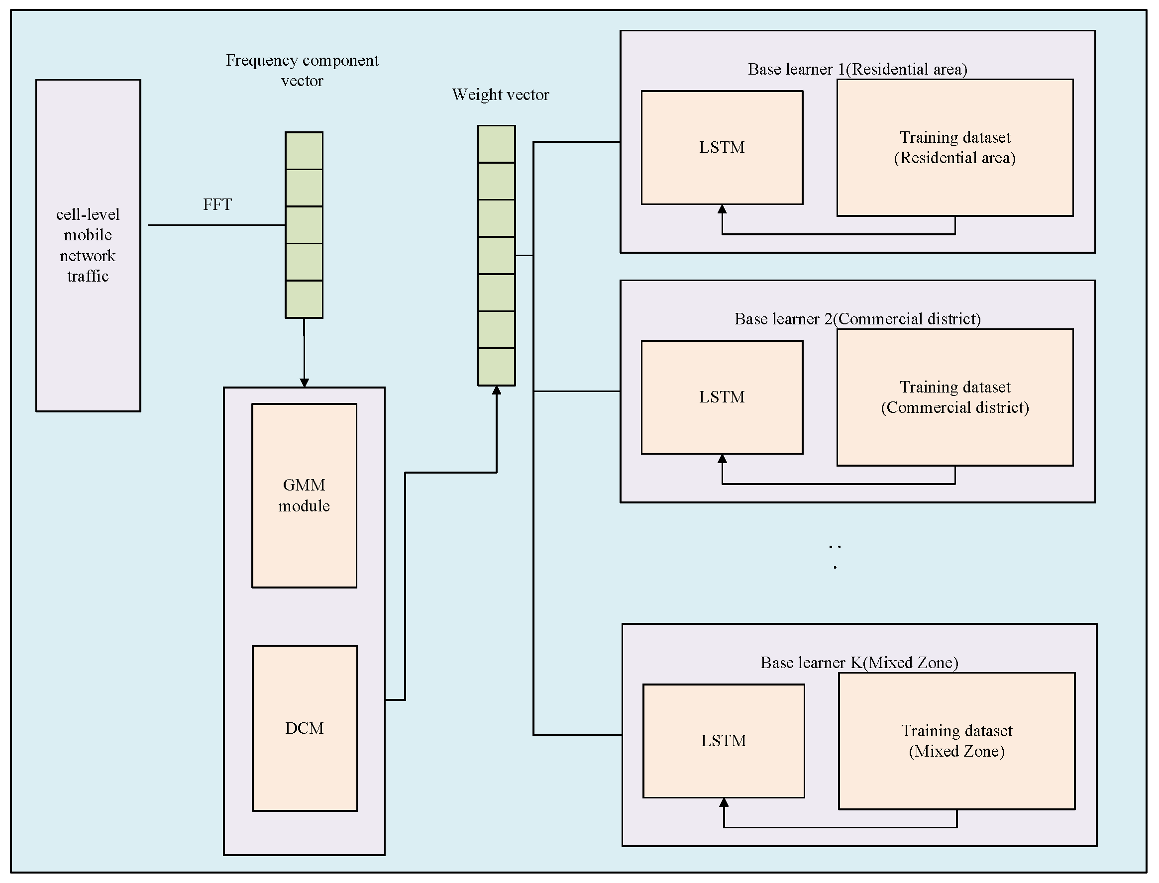
As illustrated in Figure 1, the GMM-SCM-DCM model comprises three steps. The first step subjects cellular traffic payload data to processing through operations such as the Fast Fourier Transform (FFT) to derive the traffic feature frequencies for each cellular network, which are then used to train GMMs. The second step feeds the frequency–domain features of new traffic tasks into the DCM for novelty detection. If the traffic pattern is identified as existing, the SCM mechanism assigns initial weights and executes the prediction task. If the pattern is classified as a similar pattern, it provides similarity weights and then fine-tunes using a fine-tuned dataset. If the pattern is classified as a completely new traffic pattern, a new component must be created; this step is termed component splitting. The third step utilizes the soft weights produced by the GMM to select an appropriate base learner for network traffic load prediction.

3.1. Problem Definition

This work addresses the prediction of total throughput at the base station level in 5G cellular networks, a critical input for network resource scheduling and capacity planning. We formulate the cellular traffic load prediction problem as a multivariate time series forecasting task. Consider N cellular base stations where the traffic load of each base station at time t is denoted as $x_t$. Given an observed historical sequence $X=[x_{t-T+1},\cdots ,x_t]$ of T time steps, the objective is to predict the traffic load for the next $\tau$ time steps:

$$\begin{array}{c}\hfill Y=[x_{t+1},x_{t+2},\dots ,x_{t+\tau }]=f\left(X\right|\mathrm{\Theta })\end{array}$$

(1)

where f is the prediction model and $\mathrm{\Theta }$ represents the model parameters. In the meta-learning framework, each base station or region is treated as a task $T_i$, with its training data $D_i^{train}$ and test data $D_i^{test}$. The objective of the meta-learner is to learn shared knowledge from multiple tasks, enabling new task $T_{New}$ to rapidly adapt with only a few samples:

$$\begin{array}{c}\hfill {\mathrm{\Theta }}_{New}=\mathrm{Meta}-\mathrm{Learner}(D_{new}^{train};\mathrm{\Phi })\end{array}$$

(2)

where $\mathrm{\Phi }$ is the parameter of the meta-learner.

3.2. Analysis of Dataset and Spatio-Temporal Characteristics

The experiments in this study are based on a publicly available mobile network traffic dataset collected by Telecom Italia in Milan. This dataset contains traffic records from November 2013 to January 2014, covering approximately 10,000 grid cells.

To construct a set of feature vectors suitable for this study, the time series data within the dataset was converted into frequency–domain information through the following steps:

(1)

Time series construction: The entire time span of the dataset was divided into consecutive one-hour time intervals.

(2)

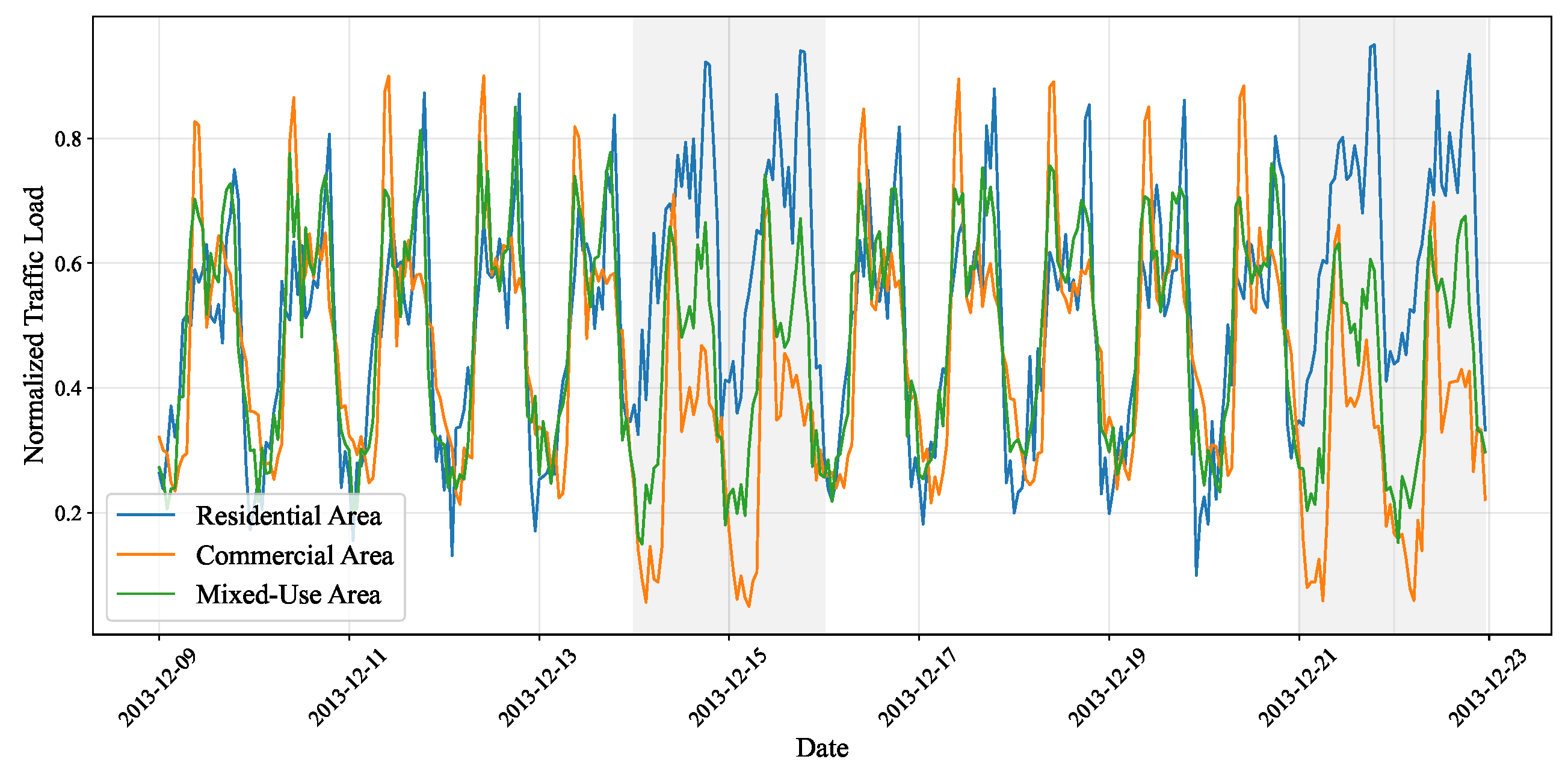
Data normalization: The traffic load was normalized to the range [0, 1] using the Min-Max algorithm. The normalized sequences distinctly reveal the diverse traffic patterns exhibited by cells across different functional zones. As illustrated in Figure 2, three representative cells display markedly different temporal characteristics during identical time periods, demonstrating the significant impact of functional differentiation within urban spaces on communication behavior. Residential areas exhibit stronger evening peak pulses (18:00–21:00), with a notable increase in baseline traffic throughout weekends. Commercial districts exhibit sharper morning peak traffic (8–11 a.m.) with markedly reduced weekend volumes. Mixed-use areas display distinct dual peaks during morning and evening hours, exhibiting moderate weekend effects.

(3)

Feature extraction: Leveraging the periodic nature of cellular network traffic, each cell’s traffic load data is treated as a discrete signal with a period $T=168$ h (one week). Its frequency domain characteristics are analyzed via Fast Fourier Transform (FFT). Five principal frequency components (corresponding to periods of 1 week, 1 day, 12 h, 8 h, and 6 h) are selected from the frequency domain information. Their real and imaginary parts collectively form a 10-dimensional feature vector:

$$\begin{array}{c}\hfill {\mathrm{\Gamma }}_p=\left[R\left(F_p(\pi /84)\right),S\left(F_p(\pi /84)\right),\right.\\ \hfill R\left(F_p(\pi /12)\right),S\left(F_p(\pi /12)\right),\\ \hfill R\left(F_p(\pi /6)\right),S\left(F_p(\pi /6)\right),\\ \hfill R\left(F_p(\pi /4)\right),S\left(F_p(\pi /4)\right),\\ \hfill \left.R\left(F_p(\pi /3)\right),\tilde{S}\left(F_p(\pi /3)\right)\right]\end{array}$$

(3)

(4)

Foundational sample construction: Formulating the traffic forecasting task as a supervised learning problem, where each foundational sample comprises data from the preceding three hours as input, with the fourth hour serving as the forecast output.

Unlike previous studies which assumed a steady-state environment, this paper focuses on the non-stationary evolution of flow patterns. To this end, we undertook a critical reconstruction and annotation of the dataset (see Section 4.4 for details), thereby establishing an evaluation benchmark that more accurately reflects genuine dynamic variations.

3.3. Probabilistic Modeling of the Feature Space

Let the feature vector for the historical baseline task be ${\left\{{\mathrm{\Gamma }}_p\right\}}_{p=1}^N\subset R^D(D=10)$, which follows a mixture model composed of K Gaussian distributions:

$$\begin{array}{c}\hfill p\left({\mathrm{\Gamma }}_p\right|\theta )=\sum _{k=1}^K{\pi }_{k}N\left({\mathrm{\Gamma }}_p\right|{\mu }_k,{\mathrm{\sum }}_k)\end{array}$$

(4)

The model parameters are $\theta ={\left\{{\pi }_k,{\mu }_k,{\mathrm{\sum }}_k\right\}}_{k=1}^K$, where ${\pi }_k$ represents the mixture coefficients in the Gaussian mixture model, denoting the probability of selecting the kth Gaussian model during data generation.

${\mu }_k$ denotes the mean of the kth Gaussian model, and ${\sum }_k$ denotes its variance. Each Gaussian distribution corresponds to a category of base station traffic features exhibiting similar traffic patterns (e.g., commercial areas, residential areas, etc.).

For the kth Gaussian component (k), the corresponding optimal set of weight vectors is

$$\begin{array}{c}\hfill W_k=\left\{w_i\right|{\mathrm{\Gamma }}_i\in {\theta }_k\}\end{array}$$

(5)

The class centers of the weight vectors are

$$\begin{array}{c}\hfill {\overline{w}}_k={\displaystyle \frac{1}{|W_k|}}\sum _{w_j\in W_k}{w}_j\end{array}$$

(6)

When inputting the meta-feature ${\mathrm{\Gamma }}_q$ for a new task q, the posterior probabilities for its membership in each component are as follows:

$$\begin{array}{c}\hfill {\gamma }_k\left({\mathrm{\Gamma }}_q\right)={\displaystyle \frac{{\pi }_{k}N\left({\mathrm{\Gamma }}_q\right|{\mu }_k,{\sum }_k)}{{\sum }_{j=1}^K{\pi }_{j}N\left({\mathrm{\Gamma }}_q\right|{\mu }_j,{\sum }_j)}}\end{array}$$

(7)

The component $k^{*}=arg{max}_k{\gamma }_k\left({\mathrm{\Gamma }}_q\right)$ with the highest posterior probability is selected, and initial weights are assigned according to the following rules.

The initial weight allocation employs an SCM, selecting the base model weight whose probability distribution most closely approximates that of the meta-feature vector as the initial weight:

$$\begin{array}{c}\hfill w_q^{init}={arg}_{w_i\in W_{k^{*}}}{∥{\mathrm{\Gamma }}_q-{\mathrm{\Gamma }}_i∥}_{{\sum }_k^{-1}}\end{array}$$

(8)

${∥·∥}_{{\sum }_k^{-1}}$ is employed to compute the Mahalanobis distance, enhancing the measurement of local similarity by introducing the covariance structure of the component $k^{*}$.

Unlike traditional GMM component learners, the number of components K in this study is not a pre-set and fixed hyperparameter. Instead, the proposed DCM mechanism (Section 3.2) dynamically adjusts the GMM structure—splitting, merging, or eliminating components—based on the novelty of patterns exhibited by new tasks. This enables the model to continuously adapt to non-stationary environments.

3.4. Dynamic Component Management Mechanism

DCM directly acts upon the meta-learner, indirectly optimizing the initialisation of the base learner by managing the evolution of GMM components. To determine whether an existing meta-learner is suitable for a new task q—i.e., whether the meta-learner requires evolution—this paper designs a dual-modal similarity metric based on probabilistic and spatial similarity. This metric primarily reflects the novelty of the traffic pattern in the traffic data stream for the new task, with specific rules as shown in the formula.

$$\begin{array}{c}\hfill \nu \left({\mathrm{\Gamma }}_q\right)=1-\underset{k}{max}{\gamma }_k\left({\mathrm{\Gamma }}_q\right)\left[exp\left(-{\displaystyle \frac{1}{D}}{∥{\mathrm{\Gamma }}_q-{\mu }_k∥}_{{\mathrm{\sum }}_k^{-1}}\right)\right]\end{array}$$

(9)

where $\nu \left({\mathrm{\Gamma }}_q\right)$ denotes the novelty metric, ${\mathrm{\Gamma }}_q$ represents the meta-feature vector for new task q, ${\gamma }_k\left({\mathrm{\Gamma }}_q\right)$ denotes the posterior probability, ${\mu }_k$ is the mean vector for component k, ${∥·∥}_{{\mathrm{\sum }}_k^{-1}}$ denotes the Mahalanobis distance, and $D=10$ represents the meta-feature dimension.

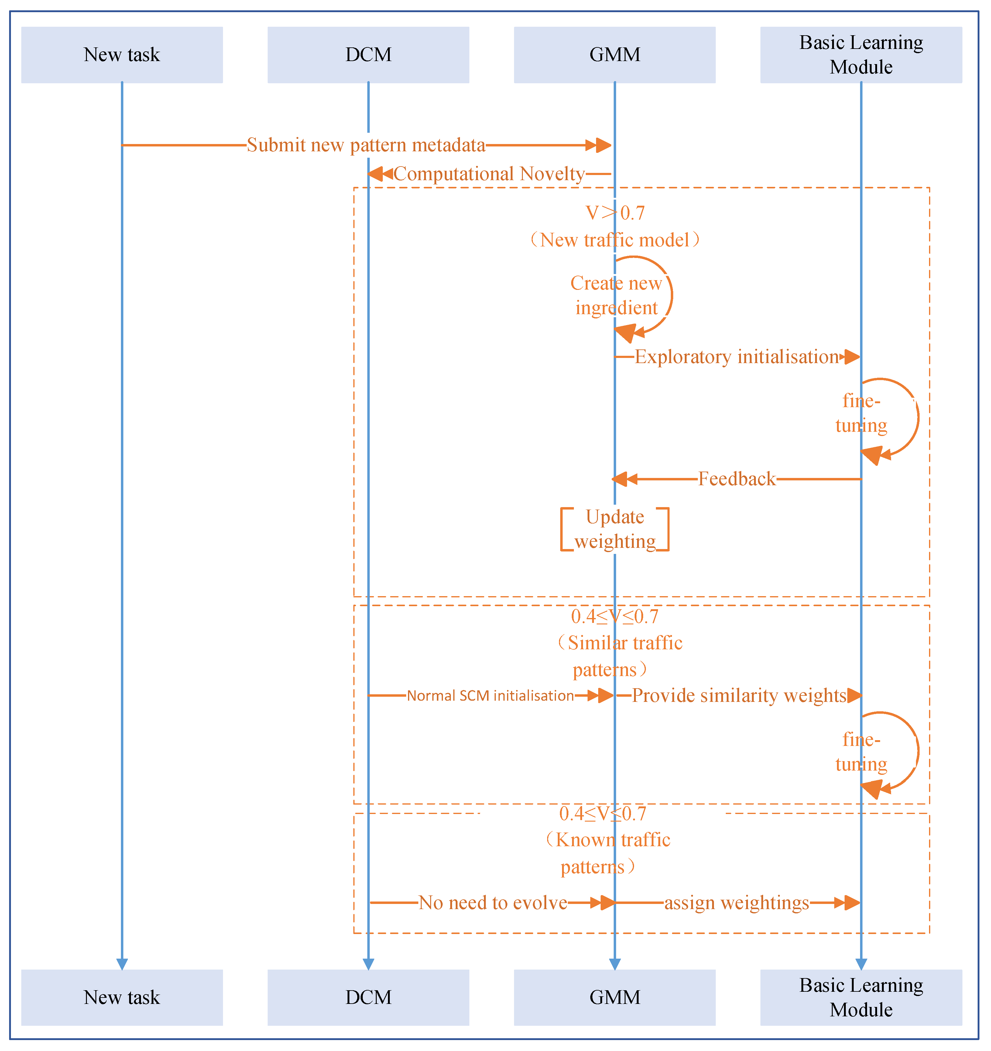
Based on the novelty metric for traffic patterns, this paper designs a three-tier response strategy utilizing DCM, as illustrated in Figure 3. When a new task requires prediction, DCM first assesses pattern novelty. If the pattern is classified as an existing traffic pattern, the SCM mechanism directly assigns initial weights and enters operational status. If judged as a similar pattern, it provides similarity weights before undergoing fine-tuning using the fine-tuning dataset. If the pattern is classified as an entirely novel traffic pattern, a new component must be created—a process termed component splitting. The specific splitting methodology is detailed in the subsequent sections.

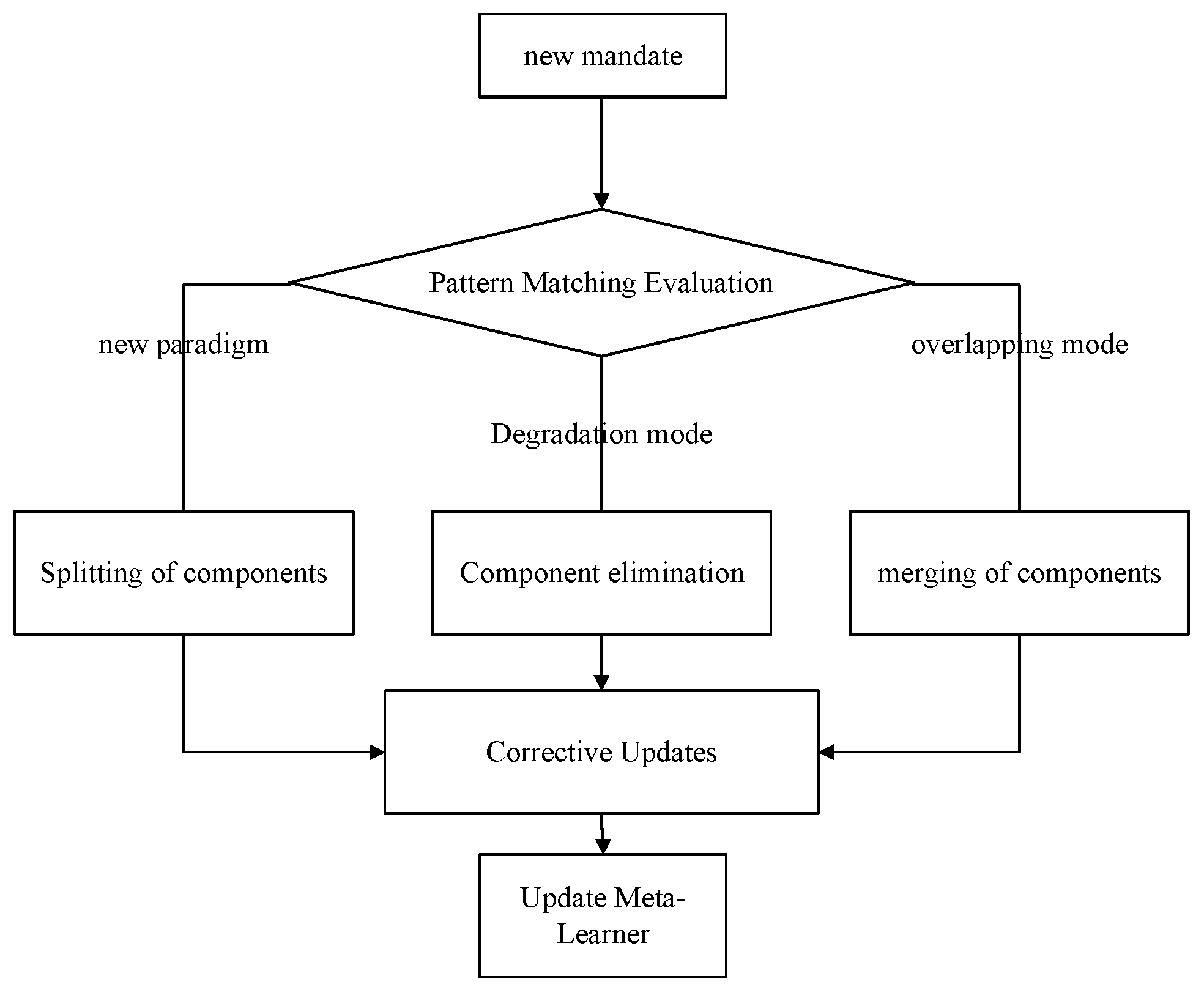
When existing components fail to meet the prediction requirements of new tasks, the DCM mechanism is triggered. Its operational flow is illustrated in Figure 4.

The splitting threshold is set at ${\tau }_{\mathrm{split}}$, the merging threshold at ${\tau }_{\mathrm{merge}}$, and the minimum survival mixture coefficient at ${\pi }_{min}$, with decisions being made via the formula.

$$\begin{array}{c}\hfill \left\{\begin{array}{cc}\mathrm{Split}\hfill & \mathrm{if}\nu >{\tau }_{\mathrm{split}}\hfill \\ \mathrm{Merge}\hfill & \mathrm{if}\underset{k}{max}{\gamma }_k<{\tau }_{\mathrm{split}}\hfill \\ \mathrm{Eliminate}\hfill & \mathrm{if}{\pi }_k<{\pi }_{min}\hfill \end{array}\right.\end{array}$$

(10)

When triggering a component splitting decision, parameters are updated as follows:

$$\begin{array}{cc}\hfill k_{\mathrm{near}}& =arg\underset{k}{min}{∥{\mathrm{\Gamma }}_q-{\mu }_k∥}_{{\sum }_k^{-1}}\hfill \\ \hfill {\mu }_{\mathrm{new}}& =\alpha {\mathrm{\Gamma }}_q+(1-\alpha ){\mu }_{k_{\mathrm{near}}}\hfill \\ \hfill \sum _{\mathrm{new}}& =\beta \sum _{k_{\mathrm{near}}}+(1-\beta )\mathrm{diag}\left({\sigma }_{\mathrm{global}}^2\right)\hfill \\ \hfill {\pi }_{\mathrm{new}}& =\eta {\pi }_{k_{\mathrm{near}}}\hfill \\ \hfill {\pi }_{k_{\mathrm{near}}}& \leftarrow (1-\eta ){\pi }_{k_{\mathrm{near}}}\hfill \\ \hfill W_{\mathrm{new}}^{*}& =w_{k_{\mathrm{near}}}^{*}+\mathcal{N}(0,{\sigma }_w^{2}I)\hfill \end{array}$$

(11)

where $k_{\mathrm{near}}$ denotes the latest component index; $\alpha$, $\beta$ represent the mean and covariance interpolation coefficients, respectively; ${\sigma }_{\mathrm{global}}^2$ denotes the global feature variance; $\eta$ denotes the mixture coefficient transfer rate; ${\sigma }_w$ denotes the weighting noise standard deviation; and $\mathcal{N}(0,{\sigma }_w^{2}I)$ denotes Gaussian noise.

When triggering component merging decisions, parameters are updated as follows:

$$\begin{array}{cc}\hfill {\pi }_{\mathrm{merged}}& ={\pi }_i+{\pi }_j\hfill \\ \hfill {\mu }_{\mathrm{merged}}& ={\displaystyle \frac{{\pi }_i{\mu }_i+{\pi }_j{\mu }_j}{{\pi }_{\mathrm{merged}}}}\hfill \\ \hfill \sum _{\mathrm{merged}}& =\sum _i{\displaystyle \frac{{\pi }_i}{{\pi }_{\mathrm{merged}}}}+\sum _j{\displaystyle \frac{{\pi }_j}{{\pi }_{\mathrm{merged}}}}+\delta {\delta }^T\hfill \\ \hfill W_{\mathrm{merged}}^{*}& ={\displaystyle \frac{{\pi }_i{W}_i^{*}+{\pi }_j{W}_j^{*}}{{\pi }_{\mathrm{merged}}}}\hfill \end{array}$$

(12)

where $\delta ={\mu }_i-{\mu }_j$ (the mean difference vector), ${\rho }_{ij}$ denotes the component similarity, $D_{\mathrm{KL}}$ represents the KL divergence, and $cos(·,·)$ stands for the cosine similarity.

When the component contribution reaches the exclusion threshold, the exclusion mechanism is triggered. The exclusion criteria are as follows:

$$\begin{array}{c}\hfill \left\{\begin{array}{cc}\hfill & {\pi }_k<{\pi }_{min}\hfill \\ {\displaystyle \frac{1}{t_c-t_0}}\hfill & {\int }_{t_0}^{t_c}{\pi }_k\left(t\right)dt<k_{min}\hfill \end{array}\right.\end{array}$$

(13)

The design of the DCM fully accounts for the dynamic characteristics of 5G networks. The operational logic can be formalized as follows:

• Component merging may correspond to the consolidation of functionally similar areas during network optimization or the decline of certain service patterns. When two components (e.g., patterns of two commercial areas) become similar due to urban development, merging them simplifies the model and prevents overfitting.
• Component elimination may correspond to the decommissioning of a base station or the obsolescence of outdated service patterns (e.g., relocation of an industrial zone). This ensures efficient utilization of the meta-learner’s resources by focusing only on currently active patterns.

3.5. Initial Weighting Mechanism for Basic Learners

In the preceding section, both the SCM and Multi-Component Mechanism (MCM) were discussed. For meta-learning traffic forecasting tasks under stationary flow patterns, selecting MCM may outperform SCM in certain scenarios. However, for non-stationary flow patterns, this study adopts a “split–merge” path based on Gaussian Mixture Models. Within this path, a bijective relationship exists between “component-flow pattern-weight set”. This bijective relationship ensures that each component corresponds uniquely to a specific flow pattern and its associated weight. The MCM’s composite weights may disrupt this bijection. In contrast, the DCM aligns more closely with the logical requirements of this path. Furthermore, MCM composite weights may induce oscillation in the evolutionary path. Consequently, this section’s research adopts the SCM as the initial weighting mechanism for the base learner, a choice grounded in both the model framework and engineering practice considerations.

The SCM mechanism operates on the principle that if the meta-features of two tasks exhibit similar probability distributions, their optimal model weights should likewise be similar. It selects the base model weight whose probability distribution most closely approximates that of the meta-feature vector as the initial weight:

$$\begin{array}{c}\hfill w_q^{\mathrm{init}}={arg}_{w_i\in W_k^{*}}{∥{\mathrm{\Gamma }}_q-{\mathrm{\Gamma }}_i∥}_{{\sum }_k^{-1}}\end{array}$$

(14)

where ${∥·∥}_{{\sum }_k^{-1}}$ is used to compute the Mahalanobis distance, incorporating the covariance structure $k^{*}$ to enhance the measurement of local similarity.

4. Experiments and Analysis

4.1. Experimental Objectives

This section aims to validate the proposed GMM-SCM-DCM meta-learning framework for non-stationary cellular traffic forecasting. This includes:

(1) Validating the effectiveness of the meta-learning initialisation strategy: Demonstrating the framework’s superiority in prediction accuracy and convergence speed compared with random initialisation, fixed initialisation, and other meta-learning approaches.

(2) Validate adaptability to non-stationary environments: By constructing a non-stationary cellular traffic test set, demonstrate that the DCM mechanism handles distribution drift more effectively than traditional methods.

(3) Validating model robustness: Testing model performance across different base learner architectures and training set sizes.

4.2. Baseline Algorithms and Parameter Settings

For a comprehensive evaluation, five categories of baseline methods are selected for comparison in this section.

(1) Traditional Statistical/Shallow Learning Methods

• SVR (RBF): Support Vector Regression with Radial Basis Function kernel. Parameters: kernel coefficient $\gamma =0.1$, regularization parameter $C=1.0$, epsilon tube $ϵ=0.1$, implemented using LIBSVM.
• SARIMA: Seasonal Autoregressive Integrated Moving Average model. Parameter configuration: $(p,d,q)=(2,1,2)$, seasonal parameters $(P,D,Q,s)=(1,1,1,24)$, where p, P represent autoregressive orders, d, D represent differencing orders, q, Q represent moving average orders, and $s=24$ indicates daily periodicity.

(2) Deep Learning Methods

• CLN-FIWV: LSTM with fixed initialisation weights. Parameters: weight initialisation using Xavier uniform distribution, learning rate $=0.001$, batch size $=8$, hidden layer dimensions $=[5,5,1]$, total trainable parameters: 428.
• CLN-RSIWV: LSTM with randomly sampled initialisation weights. Parameters: weight initialisation $\mathcal{N}(0,0.01)$, learning rate $=0.001$, batch size $=8$, hidden layer dimensions $=[5,5,1]$, and total trainable parameters: 428.

(3) Meta-Learning Methods

• ML-TP (KNN): Meta-learning framework using K-Nearest Neighbors as the meta-learner. Parameters: number of neighbors $K=3$, distance metric: Euclidean distance, weight assignment: uniform weights, feature dimension $d=10$.
• dmTP (DNN): Meta-learning framework using deep neural network as the meta-learner. Architecture: three fully connected layers $[300,300,400]$, activation function: ReLU, output dimension matches base learner’s weight dimension, optimizer: Adam with learning rate $=0.0005$.
• GMM-SCM: Gaussian Mixture Model meta-learner with Single-Component Mechanism. Parameters: number of components K selected automatically via BIC in the range $[5,50]$, covariance type: full, initialisation: K-Means++, maximum iterations $=100$.
• GMM-SCM-DCM: The complete proposed model extending GMM-SCM with a Dynamic Component Mechanism. Parameters: splitting threshold ${\tau }_{\mathrm{split}}=0.8$, merging threshold ${\tau }_{\mathrm{merge}}=0.2$, minimum survival mixture coefficient ${\pi }_{min}=0.05$, weight noise standard deviation ${\sigma }_w=0.01$, mixture coefficient transition rate $\eta =0.7$.

4.3. Parameter Settings

(1) Baseline learner configuration.

To test the robustness of the entire model, this experiment employs LSTM networks of two distinct architectures as base learners, utilizing mean squared error (MSE) as the loss function.

Table 3. LSTM architecture.

Structure	Number of Layers	Hidden Layer Dimensionality	Trainable Parameters	Learning Rate	Batch Size
I	3	[5, 5, 1]	PN = 428	0.001	8
II	4	[3, 3, 3, 1]	PN = 248

details the parameter settings for the two LSTM network architectures.

(2) Meta-learner and correction parameters

KNN model: K-nearest neighbors set to 3.

dmTP’s DNN architecture: Configuration (sets a three-layer hidden network [300, 300, 400].)

GMM model: Implemented using scikit-learn’s GaussianMixture. Number of Gaussian components K automatically selected within the range $[5,50]$ via Bayesian Information Criterion (BIC).

Feedback strength coefficient: Hyperparameter in the MCM correction mechanism $\beta$ set to 1.0.

(3) Training settings

Meta-training dataset: Primarily tested at two scales—1000 samples and 7000 samples—to validate model effectiveness under small-sample conditions.

Fine-tuning set: Simulates data scarcity scenarios, primarily testing four scales: 24, 168, 500, and 840 (corresponding to 1 day, 1 week, approximately 3 weeks, and 5 weeks of data, respectively).

Training Epochs: 100.

4.4. Dataset Construction

To reflect traffic non-stationarity, this section reconstructs stationary and non-stationary test sets based on the Telecom Italia Milan dataset. As the Telecom Italia Milan dataset does not directly provide labels such as “residential area” or “commercial area”, we must classify cells according to their traffic pattern characteristics. This study employs a data-driven unsupervised learning algorithm for clustering analysis. The core principle is that cellular traffic from different functional zones (e.g., residential, commercial) exhibits distinct, quantifiable pattern characteristics. We define a set of well-specified meta-features to characterize these patterns, apply the K-Means++ algorithm for cell clustering, and finally assign functional zone labels based on the statistical features of each cluster.

4.4.1. Feature Engineering

Using ${\mathbf{I}}_p=(I_p\left[1\right],I_p\left[2\right],\dots ,I_p\left[N\right])$ to represent the normalized traffic load time series of a cell P assuming traffic from different functional zones exhibits distinct periodic intensities and contour profiles. Based on this, we define five meta-features ${\mathbf{f}}_p\in {\mathbb{R}}^5$ to characterize each cell area:

(1)

$f_1^{\left(p\right)}$: Ratio of average weekend traffic to average weekday traffic. Typically, this ratio exceeds 1 in residential areas and falls below 1 in commercial zones.

$$\begin{array}{c}\hfill f_1^{\left(p\right)}={\displaystyle \frac{\mathrm{mean}(I_p\left[t\right]\forall t\in \left\{\mathrm{weekends}\right\})}{\mathrm{mean}(I_p\left[t\right]\forall t\in \left\{\mathrm{weekdays}\right\})}}\end{array}$$

(15)

(2)

$f_2^{\left(p\right)}$: Average traffic volume during the weekday morning peak period (e.g., 8:00–10:00).

$$\begin{array}{c}\hfill f_2^{\left(p\right)}=\mathrm{mean}(I_p\left[t\right]\forall t\in [8:00,10:00]\mathrm{on}\mathrm{weekdays})\end{array}$$

(16)

(3)

$f_3^{\left(p\right)}$: Average traffic volume during the evening peak period on weekdays (e.g., 18:00–20:00).

$$\begin{array}{c}\hfill f_3^{\left(p\right)}=\mathrm{mean}(I_p\left[t\right]\forall t\in [18:00,20:00]\mathrm{on}\mathrm{weekdays})\end{array}$$

(17)

(4)

$f_4^{\left(p\right)}$: Information entropy of the flow sequence, used to measure flow uncertainty.

$$\begin{array}{c}\hfill f_4^{\left(p\right)}=-\sum _{i=1}^{B}p\left(x_i\right){log}_{2}p\left(x_i\right)\end{array}$$

(18)

Here, we partition the range of into B equal-width bins (bins); $p\left(x_i\right)$ denotes the probability that the traffic value falls within the ith bin.

(5)

$f_5^{\left(p\right)}$: 24-h lag autocorrelation coefficient, measuring the strength of diurnal periodicity.

$$\begin{array}{c}\hfill f_5^{\left(p\right)}={\displaystyle \frac{{\sum }_{t=1}^{N-24}(I_p\left[t\right]-{\overline{I}}_p)(I_p[t+24]-{\overline{I}}_p)}{{\sum }_{t=1}^N{(I_p\left[t\right]-{\overline{I}}_p)}^2}}\end{array}$$

(19)

Compute the above five feature components for all cells to obtain the feature matrix $\mathbf{F}={[{\mathbf{f}}_1,{\mathbf{f}}_2,\dots ,{\mathbf{f}}_P]}^T\in {\mathbb{R}}^{P\times 5}$, where P denotes the total number of cells. Subsequently perform Z-score standardization to eliminate dimensional effects. Here, ${\mu }_d$ and ${\sigma }_d$ represent, respectively, the mean and standard deviation of the dth feature across all cells.

$$\begin{array}{c}\hfill {\tilde{f}}_{p,d}=(f_{p,d}-{\mu }_d)/{\sigma }_d\end{array}$$

(20)

4.4.2. K-Means++ Clustering Algorithm

This section primarily focuses on applying the K-Means++ clustering algorithm for cluster analysis. Given the standardized feature matrix $\tilde{\mathbf{F}}$, to partition P cells into K clusters $\mathcal{C}=\{C_1,C_2,\dots ,C_K\}$, minimizing the sum of squares within clusters, the problem can be defined as:

$$\begin{array}{c}\hfill \begin{array}{cccc}\hfill & \underset{\mathcal{C}}{\mathrm{minimize}}\hfill & \hfill & \sum _{k=1}^K\sum _{{\tilde{\mathbf{f}}}_p\in C_k}{\parallel {\tilde{\mathbf{f}}}_p-{\mu }_k\parallel }^2\hfill \\ \hfill & \mathrm{subject}\mathrm{to}\hfill & \hfill & \bigcup _{k=1}^K{C}_k=\{1,\dots ,P\},C_k\cap C_{k^{\prime }}=⌀\mathrm{for}k\ne k^{\prime }\hfill \end{array}\end{array}$$

(21)

where ${\mu }_k={\displaystyle \frac{1}{|C_k|}}{\sum }_{{\tilde{\mathbf{f}}}_p\in C_k}{\tilde{\mathbf{f}}}_p$ represents the centroid of cluster $C_k$.

For the aforementioned NP-complete problem, this study employs the standard K-Means algorithm combined with K-Means++ intelligent initialisation to obtain approximate solutions. K-Means++ selects initial centroids via the following probability distribution:

(1)

Randomly select the first centroid uniformly ${\mu }_1$.

(2)

For each non-cluster data point ${\tilde{\mathbf{f}}}_p$, calculate the squared distance to the nearest selected cluster center $D{\left({\tilde{\mathbf{f}}}_p\right)}^2$.

(3)

Select the next centroid probabilistically ${\displaystyle \frac{D{\left({\tilde{\mathbf{f}}}_p\right)}^2}{{\sum }_{\forall p}D{\left({\tilde{\mathbf{f}}}_p\right)}^2}}$.

(4)

Repeat steps (2) to (3) until K centers are selected.

(5)

Run standard K-Means algorithm iterations until centers stabilize or maximum iterations reached.

Finally, employing the elbow method and contour coefficient analysis, the optimal number of clusters is determined by synthesizing the peak values of both elbow points and contour coefficients.

4.4.3. Classification of Cellular Networks

Based on the calculations in Section 4.4.2, when K = 4, the following clustering results are obtained, as detailed in

Table 4. Functional explanation and label assignment for different cellular partitions.

Label	Centroid Features	Real-World Significance
Residential area	$f_1>0,f_3\gg 0,f_5>0$	High weekend traffic, pronounced evening peak, pronounced diurnal variation
Commercial district	$f_1<0,f_2\gg 0,f_5>0$	Weekend traffic low, morning peak extremely pronounced, strong diurnal variation
Mixed Zone	$f_1\approx 0,f_2>0,f_3>0$	Weekend/Weekday traffic levels comparable, exhibiting dual peak characteristics
Non-stationary zone	$f_4\gg 0,f_5<0$	High temporal entropy (disorder), weak diurnal periodicity (low autocorrelation)

. This clustering outcome provides the foundation for constructing subsequent steady-state and non-steady-state test sets.

4.4.4. Construction of the Dataset

(1) Training set

A selection shall be made from residential and commercial areas, with these two categories of cells being randomly scrambled before a 70% proportion is randomly sampled.

(2) Stationary Test Set

Select residential and commercial areas to constitute the remaining 30% of cells outside the training set. Traffic patterns in these zones exhibit pronounced, reproducible periodicity (such as morning and evening rush hours, weekend patterns) and relatively stable distribution.

(3) Non-Stationary Test Set:

Selected from all non-stationary cell areas.

As shown in

Table 5. Composition and purpose of datasets.

Dataset	Time Period	Purpose	Model Stage
Meta-training set	11-01 to 12-15	Generate samples for pre-training the foundation model	Offline meta-training
Fine-tuning set	12-16 to 12-22	Fine-tune the foundation learner to adapt to specific scenarios	Online adaptation
Test set	12-23 to 12-29	Evaluate the final performance of the optimized model	Performance evaluation

, The meta-training set comprises 70% randomly selected residential and commercial cells (Data from 1 November 2013 to 1 December 2013. The test portion consists of both stationary and non-stationary test sets, formed from the remaining 30% stationary cells and all non-stationary cells, respectively. For these test cells, this paper utilized data from 16 December 2013 to 22 December 2013 for fine-tuning, with all comparative models ultimately being evaluated using data from 23 December 2013 to 29 December 2013. This design ensures complete spatial and temporal isolation of test data from training data.

4.4.5. Simulation and Mapping of 5G Service Patterns

Although the original dataset originates from the 4G era, its diverse traffic patterns demonstrate high comparability and foresight regarding early 5G service characteristics. The four region types identified through clustering can be mapped to typical 5G scenarios:

Commercial Areas: Mapped to eMBB-dominated scenarios, characterized by sharp morning peaks on workdays with high throughput demands.

Residential Areas: Mapped to hybrid eMBB and partial mMTC scenarios, exhibiting evening peaks on workdays and stable all-day traffic on weekends, reflecting applications like home broadband and smart home devices.

Mixed-Use Areas: Represent the spatiotemporal mixture of eMBB services, constituting the most common complex scenario in urban environments.

Non-Stationary Areas: Represent traffic anomalies potentially caused by emergency events or cyberattacks, or unpredictable traffic in new service pilot zones, serving as critical testbeds for model adaptability.

Through this construction method, the non-stationary test set in this paper effectively simulates the concept drift problems caused by service dynamics and urban evolution in 5G networks.

5. Results and Analysis

5.1. Foundational Performance Evaluation

As shown in

Table 6. Performance comparison of different methods on the stabilized test set (MAE).

Algorithm	MAE	R2
SARIMA	0.1046	0.681
SVR	0.0889	0.762
Clean-RSIWV	0.0821	0.793
CLN-FIWV	0.0785	0.812
ML-TP (KNN)	0.0712	0.853
dmTP (DNN)	0.0695	0.862
GMM-SCM	0.0678	0.871
GMM-SCM-DCM	0.0682	0.868

:

(1) Under stable conditions, all meta-learning methods (KNN, DNN, GMM) still outperform traditional methods, though with more reasonable margins. For instance, the optimal meta-learning method (GMM-SCM) achieves a relative reduction of approximately 13.6% in MAE compared with the optimal traditional deep learning method (CLN-FIWV).

(2) GMM-SCM performs marginally better than KNN and DNN, demonstrating the efficacy of probabilistic modeling.

(3) GMM-SCM-DCM performed very closely to GMM-SCM (with an MAE difference of merely 0.0004), consistent with expectations. In stationary environments, the advantages of dynamic fusion are negligible and may even yield slightly inferior results to GMM-SCM due to the introduction of minor noise.

As

Table 7. Performance comparison of different methods on the non-stationary test set (MAE).

Algorithm	MAE	R2
CLN-RSIWV	0.1257	0.543
CLN-FIWV	0.1189	0.587
ML-TP (KNN)	0.1033	0.658
dmTP (DNN)	0.0976	0.692
GMM-SCM	0.0921	0.721
GMM-SCM-DCM	0.0835	0.773

indicates:

(1) In non-stationary environments, all methods exhibit significant performance degradation, with MAE generally increasing and R² markedly decreasing, which aligns with expectations for non-stationary flow forecasting tasks.

(2) The advantage of GMM-SCM-DCM becomes more pronounced. MAE is reduced by approximately 9.3% compared with GMM-SCM and improves by approximately 14.4% over the best baseline method (dmTP).

(3) KNN and DNN meta-learners exhibited severe performance degradation, as they struggled to handle novel patterns (non-stationarity) unseen in the training set. Conversely, the GMM-SCM-DCM model demonstrated superior generalization capability and robustness through its probabilistic framework and the dynamic weighting of DCM.

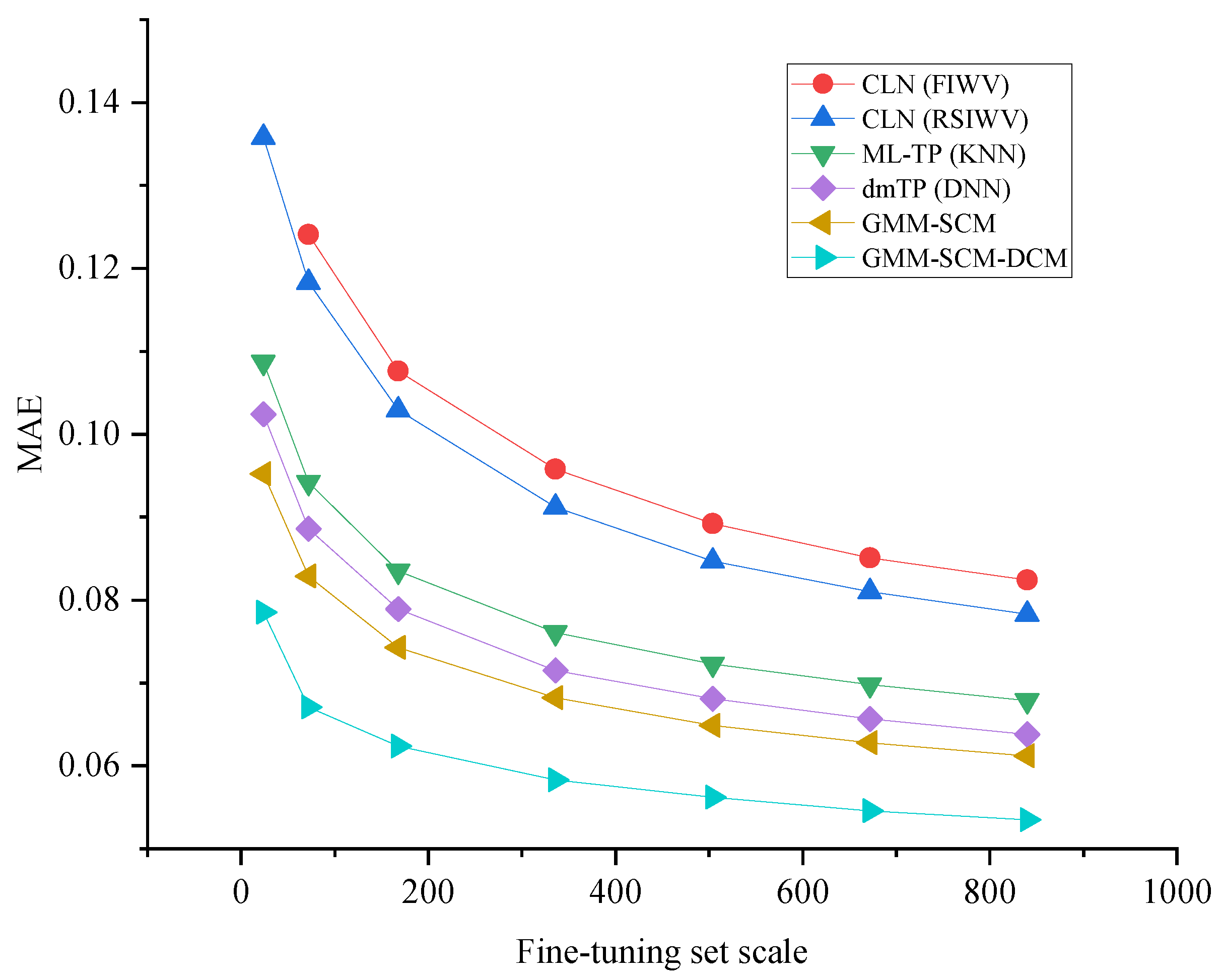
Figure 5 illustrates the impact of fine-tuning dataset scale on performance (non-stationary test set). As shown in Figure 5, the CLN-RSIWV and CLN-FIWV curves exhibit the highest performance, declining only gradually with increasing data volume. The KNN, DNN, and GMM-SCM curves occupy intermediate positions. The GMM-SCM-DCM curve consistently remains at the bottom, maintaining low error even with minimal data, demonstrating robust performance under small-sample conditions. As data volume increases, all curves gradually converge, but GMM-SCM-DCM ultimately achieves the best performance.

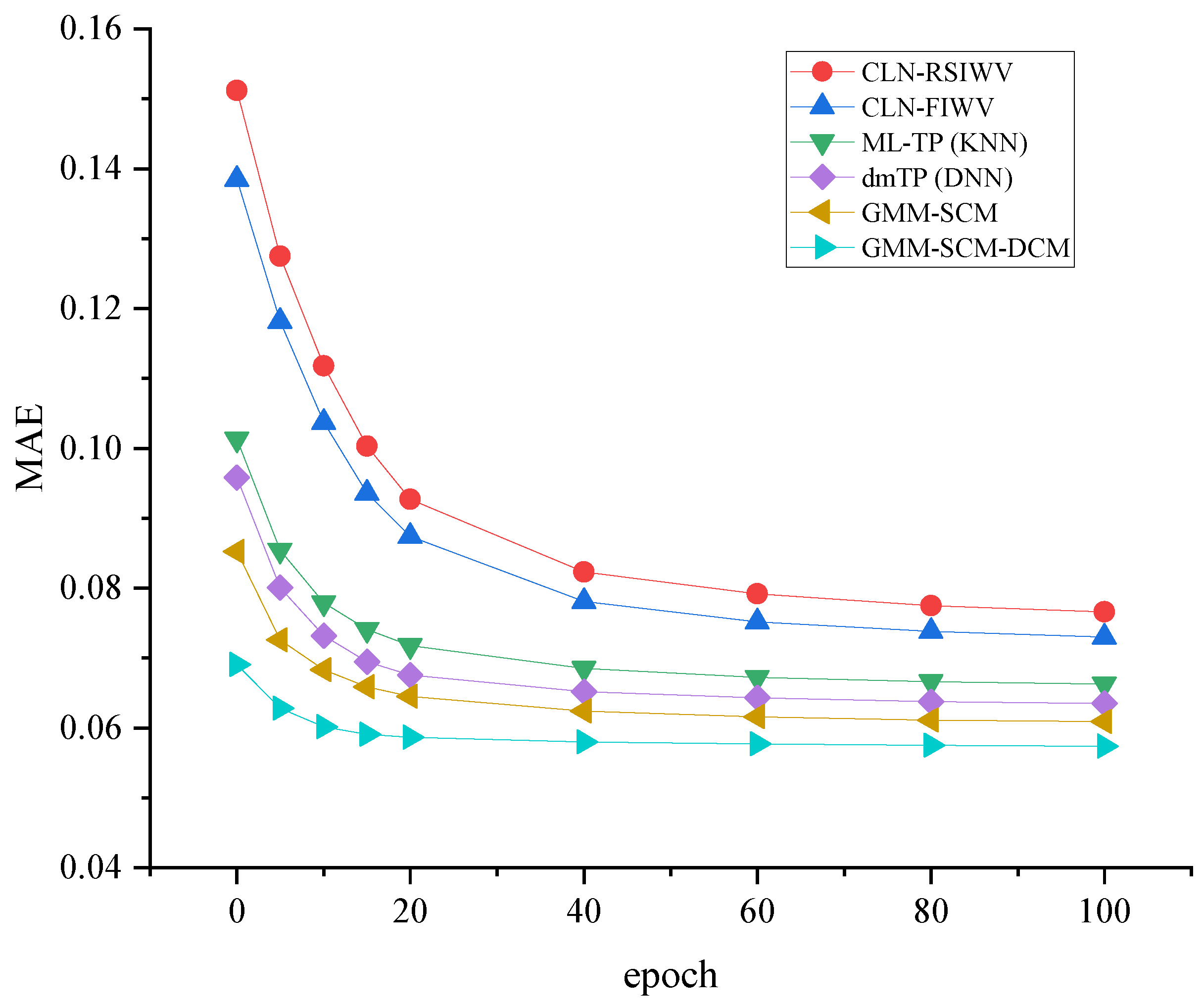
Figure 6 illustrates the convergence behavior of different models. As shown, the error curve for the CLN method starts from an extremely high value and requires approximately 80 iterations to converge slowly. GMM-SCM begins at a lower starting point. GMM-SCM-DCM exhibits the lowest starting point and converges rapidly to a stable state within approximately 10–15 iterations, demonstrating that its initial weights are very close to the optimal solution and effectively enhancing training efficiency.

5.2. Model Robustness Testing

To demonstrate that the proposed framework is independent of specific base learner architectures and maintains stable performance across varying data scales, this section conducts robustness testing using a non-stationary test set.

Analysis of the results in

Table 8. Robustness testing based on different base learners and training scales.

Training Set Size	Base Learner	MAE (GMM-SCM-DCM)	MAE (CLN-FIWV)
1000	LSTM	0.0871	0.1250
	GRU	0.0865	0.1245
4000	LSTM	0.0840	0.1205
	GRU	0.0835	0.1200
7000	LSTM	0.0835	0.1189
	GRU	0.0829	0.1182

reveals that regardless of whether the base learner employs LSTM or GRU, the GMM-SCM-DCM framework consistently and significantly outperforms the conventional initialisation method (CLN-FIWV). GRU, owing to its fewer parameters and simpler structure, exhibits a marginal advantage under the limited data conditions of this experiment. This indicates that the proposed meta-learning framework constitutes a generalized architecture whose effectiveness is independent of specific underlying network choices, demonstrating robust performance.

Figure 7 illustrates the sensitivity of different models to meta-training set size. As shown, dmTP (DNN) performance is highly dependent on the number of meta-training samples, even underperforming KNN at 1000 samples before improving with increased data. GMM-SCM and GMM-SCM-DCM demonstrate robust performance even with small meta-training sets, exhibiting stable improvement with increasing data volume. This validates the superior data efficiency and small-sample meta-learning capabilities of the GMM-SCM-DCM model.

Moreover, the performance of all models improves with an increase in the meta-training set size. Notably, even under extremely small sample conditions (1000 samples), GMM-SCM-DCM still provides high-quality initialisation, significantly outperforming traditional methods with larger datasets (7000 samples).

5.3. Ablation Studies

To validate the effectiveness of the proposed DCM and SCM mechanisms individually, as well as their synergistic effect when combined, ablation experiments were conducted on non-stationary traffic datasets. The comparison models are as follows:

GMM-MCM-DCM: Employing the Multi-Component Mechanism in place of SCM as the negative control group.

(GMM-SCM (Static): employs the SCM mechanism but disables DCM functionality (i.e., the number of GMM components remains fixed and is not dynamically adjusted). This group serves to validate the role of DCM.)

GMM-SCM-DCM (Ours): This paper’s proposed complete model.

The results of the ablation experiments are shown in

Table 9. Ablation experiment results.

Model Variants	MAE	R2	Epochs
GMM-MCM-DCM	0.0952	0.698	45
GMM-SCM	0.0898	0.735	25
GMM-SCM-DCM	0.0835	0.773	15

. Analysis reveals:

GMM-MCM-DCM vs. GMM-SCM-DCM (Static): GMM-MCM-DCM (exhibited the poorest performance (highest MAE, lowest R²), coupled with slow convergence. This validates this paper’s view: under multi-component fusion mechanisms, synthetic weights disrupt the bijective relationship between “component-pattern-weight set“, causing training oscillations and performance degradation, demonstrating the efficacy and necessity of the SCM mechanism.

GMM-SCM vs. GMM-SCM-DCM: Disabling DCM resulted in a noticeable decline in model performance on the non-stationary test set (MAE increased from 0.0835 to 0.0898), alongside requiring more iterations to converge. This indicates that when confronted with novel patterns unseen in the training set, the fixed GMM structure fails to effectively characterize and adapt, leading to a performance bottleneck. This directly demonstrates the core contribution of the DCM mechanism in addressing non-stationarity.

Overall, GMM-SCM-DCM achieved optimal performance, demonstrating the synergistic effect of SCM and DCM mechanisms: SCM ensures precise initialisation within components, while DCM ensures the component structure can dynamically evolve to adapt to external changes.

5.4. Cross-Dataset Generalization Capability Validation

This section’s experiments validate the GMM-SCM-DCM framework’s performance on another independent public dataset, demonstrating its effectiveness is not dataset-specific and possesses strong generalization capabilities.

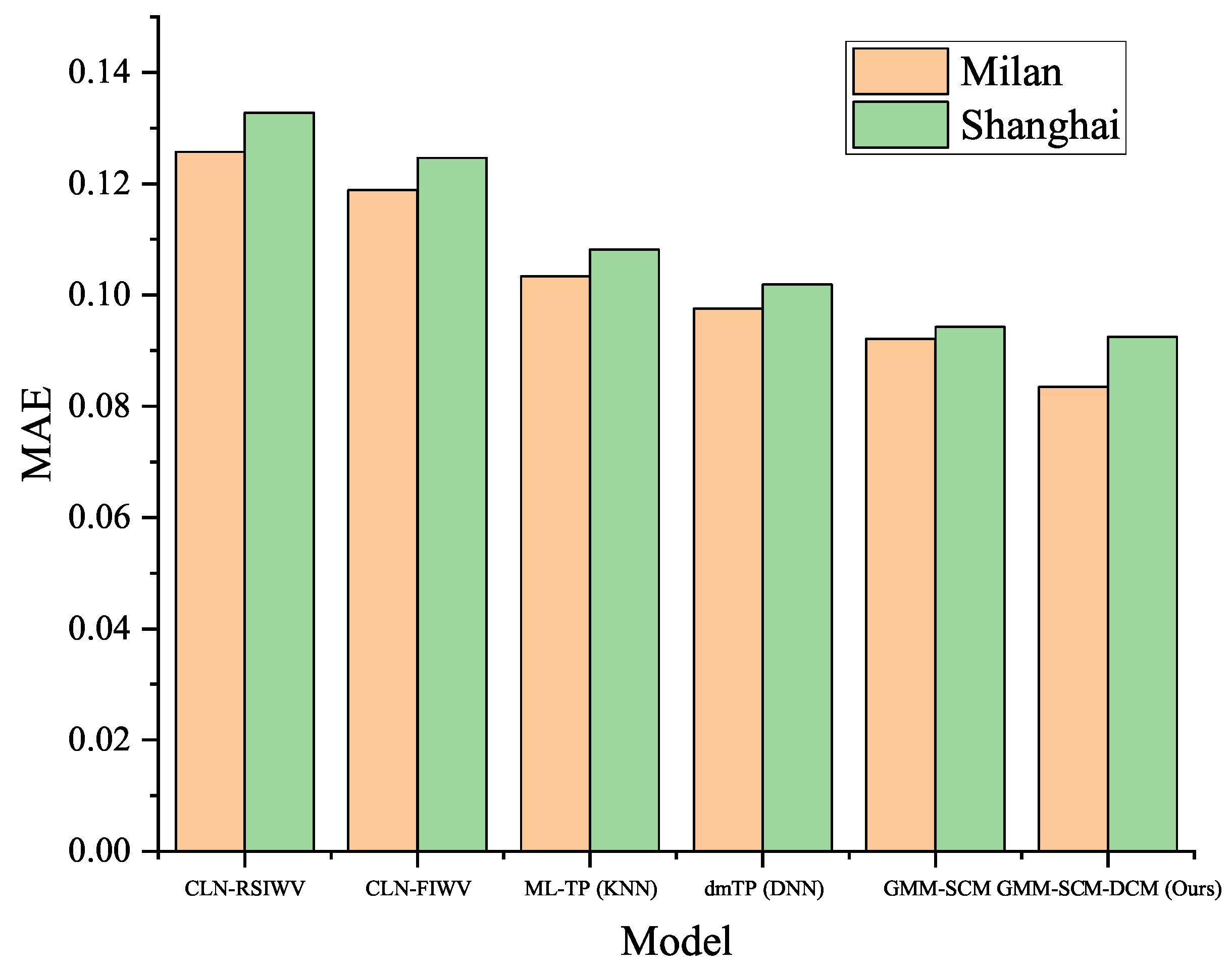
The dataset selected for this section’s experiments is the Telecom Shanghai Dataset. Like Telecom Italia, this dataset is another commonly used public benchmark dataset within the field. Data preprocessing procedures are consistent with those applied to the Telecom Italia dataset.

As shown in

Table 10. Performance of different models on the Shanghai Dataset (MAE).

Model	MAE (Shanghai)	R2 (Shanghai)
CLN-RSIWV	0.1328 (+0.0071)	0.501
CLN-FIWV	0.1246 (+0.0057)	0.561
ML-TP (KNN)	0.1082 (+0.0049)	0.631
dmTP (Deep Neural Network)	0.1019 (+0.0043)	0.664
GMM-SCM (Static)	0.0943 (+0.0022)	0.708
GMM-SCM-DCM (Our Method)	0.0925 (+0.0036)	0.732

and Figure 8, the GMM-SCM-DCM framework demonstrated exceptional robustness when confronted with the more complex distribution and potentially higher noise levels of the Shanghai dataset. Although all models exhibited varying degrees of performance degradation, GMM-SCM-DCM still delivered superior results, indicating it is a highly reliable, versatile, and robust framework.

5.5. Visualization of GMM Component Dynamic Evolution Process

The objective of this section’s experiments is to visually demonstrate the DCM mechanism’s management of the entire lifecycle of GMM components (generation, splitting, merging, and elimination) within a long-duration simulated task flow, thereby validating its capability to handle non-stationary traffic fluctuations.

Using non-stationary flow to create a simulated scenario:

Initial stable period (T0–T50): The model has learned through the meta-training set two stable patterns: ”commercial zone” (marked by morning rush hour) and “residential zone” (marked by evening rush hour).

Non-stationary zone emerges (T50–T100): A large-scale construction project (e.g., new underground station) commences in one area, causing its traffic flow to lose periodicity and become disordered with violent fluctuations. The DCM must recognize this as a new “non-stationary zone” pattern.

Functional evolution resulting information of hybrid zones (T100–T200): An original “commercial zone” gradually evolves in function due to the completion of surrounding residential buildings, beginning to exhibit characteristics of both morning and evening rush hours. The DCM must detect this change and merge the old commercial pattern with the new hybrid pattern.

Figure 9 clearly demonstrates the DCM mechanism’s pivotal role in addressing non-stationary evolution of urban functions, specifically:

Capturing new non-stationary patterns (T = 75): When construction zones induce non-stationary flow patterns (high entropy values, weak periodicity), existing commercial and residential components could not adequately characterize these patterns. The DCM generated a new component (Comp.3) via splitting operations, whose weight steadily increased, demonstrating the model’s successful identification and adaptation to this abrupt change.

Adapting to functional evolution (T = 175): As an area evolves from purely commercial to mixed use, its flow characteristics begin incorporating both morning and evening peak periods. DCM detects feature overlap and convergence between the original commercial component (Comp.1) and the emerging mixed use pattern, triggering a merging operation. The original commercial component is absorbed, with a new, more accurate mixed use Component (Comp.4) becoming dominant, optimizing the model structure and eliminating redundancy.

Clearing extinct patterns (T = 250): A residential zone component (Comp.2) experiences persistently declining traffic activity, its weight eventually falling below the minimum survival threshold. DCM then triggers an elimination mechanism, removing this component to concentrate model resources on currently active patterns.

Achieving a new steady state: Ultimately, the model is dominated by Comp.3 (non-stationary zone) and Comp.4 (mixed zone), accurately reflecting the city’s entirely new functional state following its evolution.

5.6. Computational Complexity Analysis

This section provides both theoretical analysis and experimental comparison of the computational complexity for the proposed method and baseline algorithms during both training and inference phases.

Theoretical Analysis:

SARIMA: Time complexity is $O\left((p+q+P+Q)L^2\right)$, where p, q are non-seasonal AR and MA orders, P, Q are seasonal AR and MA orders, and L is the sequence length. Space complexity is $O\left(L\right)$.

SVR: Training using the sequential minimal optimization algorithm has complexity between $O\left(n^{2}d\right)$ and $O\left(n^{3}d\right)$, where n is the number of samples and d is the feature dimension. Inference complexity is $O\left(n_{s}d\right)$, where $n_s$ is the number of support vectors.

LSTM (CLN-RSIWV/FIWV): Training complexity is $O(T·L·h^2+T·h·h_{in})$, where T is the sequence length, L is the number of LSTM layers, h is the hidden dimension, and $h_{in}$ is the input dimension. The complexity for a single time step forward pass is $O(h_{in}h+h^2)$.

ML-TP (KNN): Training only requires storing meta-features with complexity $O\left(1\right)$. Inference requires computing similarities between the new task and all historical tasks with complexity $O\left(Nd\right)$, where N is the number of tasks and d is the feature dimension.

dmTP (DNN): Training complexity is $O(E·B·{\sum }_{l=1}^L{h}_{l-1}{h}_l)$, where E is the number of epochs, B is the batch size, L is the number of layers, and $h_l$ is the number of neurons in layer l. Inference complexity is $O\left({\sum }_{l=1}^L{h}_{l-1}{h}_l\right)$.

GMM-SCM: Training using the Expectation Maximization algorithm has per-iteration complexity $O\left(KN{d}^2\right)$, where K is the number of components, N is the number of samples, and d is the feature dimension. Inference complexity for computing posterior probabilities is $O\left(K{d}^2\right)$.

GMM-SCM-DCM: The training complexity is the same as GMM-SCM. During online adaptation, the DCM mechanism adds operations for pattern novelty detection and component management: pattern novelty detection complexity $O\left(K{d}^2\right)$, component splitting $O\left(d^3\right)$, component merging $O\left(K{d}^2\right)$, and component elimination $O\left(K\right)$.

Experimental Results:

All models were evaluated under identical hardware conditions, recording average training and inference times on the non-stationary test set. The test set contains 100 tasks, each comprising 168 h (1 week) of traffic data with a time slot length of 1 h. Experimental results are shown in

Table 11. Computational efficiency comparison of different models.

Model	Training Time (s)	Inference Time (ms/Sample)
SARIMA	12.3	5.67
SVR	8.9	2.34
CLN-RSIWV	45.2	1.89
CLN-FIWV	42.9	1.85
ML-TP (KNN)	0.05	3.45
dmTP (DNN)	120.5	2.11
GMM-SCM	18.7	1.52
GMM-SCM-DCM	22.3	1.63

.

The experimental results show that traditional statistical methods (SARIMA, SVR) have advantages in training and inference speed but limited prediction accuracy. Deep learning methods (CLN series) require longer training times but offer fast inference. Among meta-learning methods, the KNN meta-learner has the fastest training but slower inference; the DNN meta-learner has the highest training complexity; and GMM-based methods achieve a good balance between training and inference efficiency. GMM-SCM-DCM significantly improves prediction accuracy and adaptation capability in non-stationary environments with only a modest increase in computational overhead (approximately 19% increase in training time and 7% increase in inference time compared with GMM-SCM), demonstrating good engineering feasibility.

Furthermore, this paper analyzes the relationship between computational complexity and task scale for each model. As the number of tasks N increases, the inference time of the KNN meta-learner grows linearly ($O\left(N\right)$), while the inference time of GMM-based methods remains stable ($O\left(1\right)$), making them more suitable for large-scale deployment scenarios.

6. Conclusions

The experiments in this chapter demonstrate that the GMM-SCM-DCM model outperforms traditional deep learning methods and other meta-learning baseline algorithms in cellular traffic forecasting tasks, whether for stationary or non-stationary traffic, in terms of prediction accuracy, convergence speed, and robustness.

Analysis reveals that within the GMM-SCM-DCM framework, the GMM provides probabilistic modeling of weight distributions, offering greater interpretability and statistical efficiency than KNN and DNN. SCM delivers precise initialisation under stationary conditions. DCM is pivotal for handling non-stationary traffic, with its dynamic fusion mechanism significantly enhancing the model’s generalization capability and robustness. This framework is particularly suited for scenarios involving new base stations or sudden events, where historical data is scarce or diverges substantially from past patterns, rendering traditional methods ineffective. Our approach enables rapid provision of high-quality initialisation, achieving an efficient “cold start”.

The findings of this research not only present a novel and efficient meta-learning solution for cellular network traffic forecasting but also offer valuable insights and implementation pathways for broader non-stationary time series prediction challenges. Moving forward, we shall further explore integrating the DCM mechanism with paradigms such as online learning and continuous learning to enhance the model’s adaptability and stability within long-term evolving environments.

The findings of this study not only provide an efficient meta-learning solution for cellular network traffic prediction but also offer valuable modeling insights and implementation pathways for broader non-stationary time series forecasting problems. Although GMM-SCM-DCM demonstrates excellent performance in non-stationary traffic prediction, several promising research directions remain:

Online and continual learning: Integrating the DCM mechanism with online learning frameworks to achieve lifelong learning on continuously arriving data streams while mitigating catastrophic forgetting.

Federated meta-learning: Extending the proposed framework to federated learning environments, enabling collaborative meta-learning across cellular networks under data privacy constraints.

Interpretability and visualization: Incorporating explainable AI techniques (e.g., SHAP, LIME) to provide visual interpretations of the meta-learner’s component assignment and pattern evolution processes.

Cross-modal fusion: Enhancing the perception and prediction capability for non-stationary patterns by incorporating external multimodal data (e.g., meteorological, social events, traffic flow).

Lightweight design and edge deployment: Optimizing the model architecture and component management strategies to adapt to the resource constraints of edge computing devices, enabling real-time prediction on the end side.

Future work will focus on these directions to further enhance the model’s applicability and intelligence in practical network environments.