Fast Resource Estimation of FPGA-Based MLP Accelerators for TinyML Applications

Abstract

Tiny machine learning (TinyML) demands the development of edge solutions that are both low-latency and power-efficient. To achieve these on System-on-Chip (SoC) FPGAs, co-design methodologies, such as hls4ml, have emerged aiming to speed up the design process. In this context, fast estimation of FPGA’s utilized resources is needed to rapidly assess the feasibility of a design. In this paper, we propose a resource estimator for fully customized (bespoke) multilayer perceptrons (MLPs) designed through the hls4ml workflow. Through the analysis of bespoke MLPs synthesized using Xilinx High-Level Synthesis (HLS) tools, we developed resource estimation models for the dense layers’ arithmetic modules and registers. These models consider the unique characteristics inherent to the bespoke nature of the MLPs. Our estimator was evaluated on six different architectures for synthetic and real benchmarks, which were designed using Xilinx Vitis HLS 2022.1 targeting the ZYNQ-7000 FPGAs. Our experimental analysis demonstrates that our estimator can accurately predict the required resources in terms of the utilized Look-Up Tables (LUTs), Flip-Flops (FFs), and Digital Signal Processing (DSP) units in less than 147 ms of single-threaded execution.

1. Introduction

The increasingly stringent power and performance requirements of Internet-of-Things (IoT) applications has led to a shift towards moving processing at the edge on near and in-sensor devices to minimize the data communication latency and power expenses and ensure privacy [1]. This demand has given rise to the tiny machine learning (TinyML) paradigm, wherein machine learning (ML) inference models are executed on resource-frugal devices with low memory and processing footprints [2]. Given the requirements for energy efficiency and low-latency processing, system-on-chip (SoC) FPGAs are considered ideal computing platforms for the TinyML field due to their flexibility, non-recurring engineering cost (NRE), fast design time compared to ASICs [3], and their power efficiency compared to CPU and GPGPU systems [1].

In the past, the programming model of FPGAs was entirely based on register-transfer level (RTL) descriptions. However, nowadays the shrunk time-to-market (TTM) window has led to the adoption of high-level synthesis (HLS) techniques [4] and co-design methodologies [5,6] to speed up the design process. In this context, the rapid estimation of a design’s feasibility is crucial in the TinyML field, where the contradictory requirements of ultra-resource-constrained devices and demands for high-performance computations make many design choices impractical [7]. In FPGA accelerators designed for TinyML applications, the neural network’s coefficients can be directly hardwired in the circuit’s description resulting in the design of fully customized (bespoke) circuits optimized for the application’s requirements. Such fully customized circuits offer unmatched energy and latency efficiency [8]. This approach is followed by hls4ml [5], a state-of-the-art framework for designing highly parallel ML models on resource- and power-constrained FPGA platforms [2,9].

In this manuscript, we present a methodology for the rapid and precise enough estimation of the resource utilization of bespoke multilayer perceptrons (MLPs) designed with the hls4ml [5] workflow and deployed on resource-constrained FPGAs. MLPs consist one of most commonly used ML algorithms in TinyML applications [10,11,12]. Bespoke MLP implementation on small devices requires many design iterations due to the circuits’ high parallelism and customization [5]. Our methodology estimates the MLP’s resource utilization given the model’s topology, the accelerator’s architecture, and the network’s coefficients without relying on the model’s RTL description or HLS code. The inputs to our estimator are directly derived from the model’s high-level description through the hls4ml flow. As a result, our proposed resource estimator can be utilized by designers or ML engineers to assess the feasibility of their designs without executing the HLS first, thus exploring the respective design space quickly at a high level. For example, our estimator can serve as the backbone of hardware-aware neural architecture search (NAS) frameworks targeting TinyML on FPGAs [13].

Our estimator is evaluated on six different design architectures used in hls4ml for bespoke synthetic and TinyML benchmark MLPs on Xilinx SoC FPGAs. On average, the required look-up tables (LUTs) and flip-flops (FFs) are estimated with higher than $88\%$ and $90\%$ accuracy, respectively, while the digital signal processing (DSP) units are precisely estimated. The execution time of our estimator did not exceed $147\mathrm{ms}$. Our estimator is built upon the state-of-the-art hls4ml framework [5] and is made publicly available (https://github.com/ArgyKokk/hls4ml_MLP_estimator (accessed on 6 January 2025)). To the best of our knowledge, this is the first resource estimator for FPGA-based bespoke MLP implementations targeting TinyML.

The rest of this manuscript is organized as follows. Section 2 presents an overview of the TinyML domain; state-of-the-art co-design methodologies of machine learning (ML) accelerators on FPGAs are discussed along with proposed resource estimators. Next, in Section 3, our proposed resource estimation methodology is analyzed. In Section 4, the resource estimator’s experimental results are presented. Finally, in Section 5, the paper is concluded.

2. Background and Related Work

Tiny machine learning (TinyML), a term introduced by Warden et al. in 2021 [11,14], refers to machine learning (ML) applications that can be trained without the need for highly parallel processing hardware (e.g., GPUs, multi-core CPUs). These applications can be deployed on ultra-low-power low-cost microcontrollers at the edge [15], democratizing ML and allowing users from diverse backgrounds to rapidly deploy simple “always-on” models on battery-powered devices. Typical use cases include industrial predictive maintenance, analytics, and environmental monitoring [14]. TinyML emerged through a collaborative educational initiative involving academia and industry (Harvard and Google [16]). Today, the field spans multiple domains such as healthcare, robotics, and transportation [14].

Initially, TinyML efforts focused on the implementation of ML models on microcontrollers and educational platforms such as Arduino. However, recent advancements in high-level synthesis (HLS) tools for FPGAs, together with co-design frameworks such as FINN [6] and hls4ml [5], have extended TinyML to FPGA-based solutions [17]. These frameworks facilitate the conversion and compression of PyTorch and Keras models into HLS descriptions, enabling ultra-low-latency energy-efficient inference in resource-constrained contexts.

Hls4ml is used to design low-latency neural networks on FPGAs. It incorporates Qkeras [18] to support network compression and efficient edge deployments [19]. Furthermore, its architecture, which parallelizes at different degrees the multiply–accumulate (MAC) operations, allows layers to run in as few as one clock cycle [5]. A 2021 benchmarking study by industry and academia (e.g., Harvard, Fermilab, Google, Columbia) identified hls4ml as the most popular framework for FPGA-based ML deployment [20], while a 2022 review indicated that Xilinx PYNQ FPGA devices are currently the most commonly used FPGA platforms in TinyML [21].

Several other frameworks have been proposed to enable hardware-efficient ML inference on FPGAs. In 2016, Wang et al. proposed DeepBurning [22], one of the first frameworks aiming to enable the semi-automatic generation of hardware-efficient RTL descriptions of neural networks (NNs) on FPGAs. In [23], they introduced a scheme to generate fully pipelined convolutional neural network (CNN) architectures by mapping weights to on-chip memory. Although this strategy is effective, it was demonstrated on larger FPGA platforms (e.g., Intel Stratix V, Xilinx Artix 7) that are less suited to the resource constraints typically encountered in TinyML. In [24], a framework was proposed for pipelining deep neural network (DNN) architectures, but it relied on continuous communication with external memory, limiting performance due to DRAM bandwidth constraints, which causes execution stalls and higher latency. In contrast, ref. [25] targeted resource-constrained FPGAs by using iterative quantization, pruning, and MAC reuse across DSPs; like [23], it also stores network coefficients on-chip to reduce off-chip data transfers and energy consumption, while in [26], they follow streaming architecture strategies to minimize latency without compromising the design’s feasibility. In [27], a design methodology of FPGA MLP accelerators that enables the sharing of the multiplication units among different neurons is suggested to minimize the utilized multipliers.

Most FPGA accelerators use the off-chip DRAM memory to fetch the network’s coefficients in the programmable region to perform computations. However, the latency and power overhead induced by the communication with the off-chip memory is prohibitive for applications with strict energy and performance requirements [8]. Hardwiring the network’s coefficients in the programmable logic and designing fully customized accelerators comprise an efficient solution, followed by [5,8,23,25,28]. However, such bespoke implementations significantly increase the resource utilization and require model compression to enable their implementation on resource-constrained devices [7]. To validate the feasibility of each accelerator on the target platform, the HLS estimator must first be executed. Depending on the network’s size, architecture, and hardware, this process can take several hours to generate an estimation report [4], leading to prolonged design cycles.

Resource utilization estimators have been proposed in [4,29,30,31,32,33,34,35,36,37,38]. However, none of these works can be directly applied to estimate resource utilization in bespoke architectures, as they do not consider the peculiarities of hardwiring a design’s parameters into the circuit’s description, such as weight sharing [39], which in such fully customized architectures is an optimization that is performed directly by the HLS compiler, during the development of their estimation models. Instead, these methods typically follow one of three approaches. Some construct dynamic data dependence graphs (DDGs) from runtime traces to make estimations for different optimization directives (e.g., pipelining, unrolling) before the accelerator’s RTL descriptions are generated [30]. Others use regression models [31,32,37,38] or estimation models by first processing the HLS code through source-to-source transpilers [29,33,34], while others rely on the circuit’s RTL description [35,36]. However, in bespoke implementations, where network coefficients are hardwired into the multipliers’ descriptions, resource utilization is influenced not only by the accelerator’s architecture but also by the specific values of the network’s coefficients. Therefore, accurately determining the resources utilized by the accelerator’s neurons requires evaluating these weight values in addition to the architectural design.

3. Proposed Resource Estimator

Our proposed resource estimator predicts the number of LUTs, FFs, and DSPs that are required for the implementation of fully connected layers, given their topology, weights, biases, and their design architecture as generated by hls4ml.

3.1. LUTs and DSPs Estimator

First, to build the LUTs and DSPs estimator, it is crucial to analyze how the bespoke multiplications and the accumulations are handled by HLS for different implementation approaches and architecture types. This analysis is presented in Section 3.1.1 and Section 3.1.2 below.

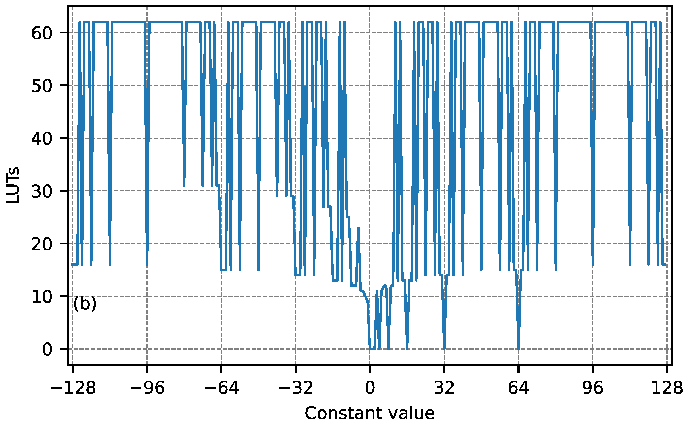
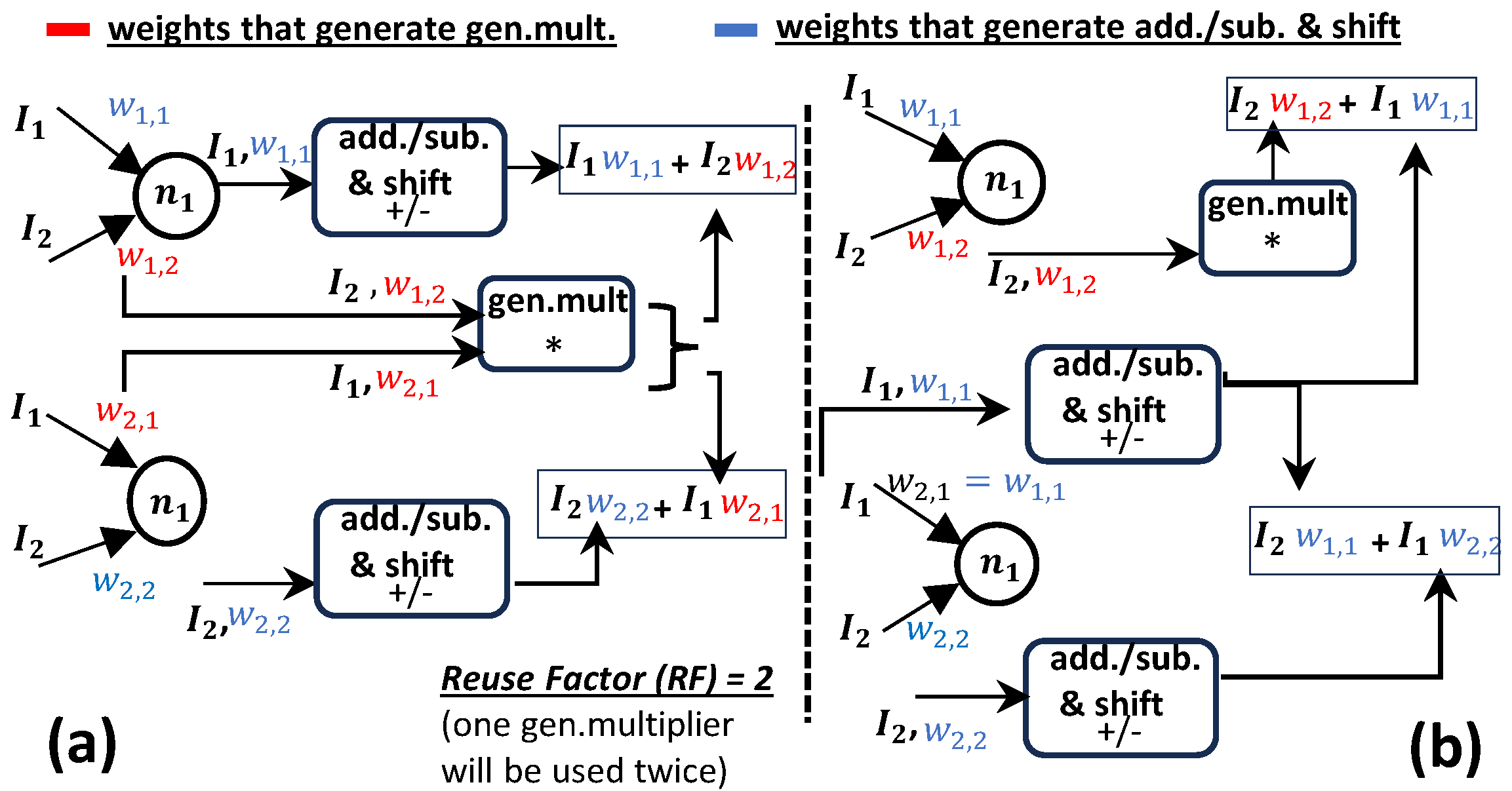
3.1.1. Multiplication in Bespoke MLPs

In bespoke designs, the number of LUTs needed for a multiplication depends on the operands’ values, as HLS may perform multiplications with addition/subtraction modules and shift operations. Specifically, depending on the operands’ values, HLS infers either generic multiplier modules that are implemented on DSPs/LUTs or modules for additions/subtraction (add./sub.) that are implemented in LUTs. In architectures that are pipelined or fully serial, the generic multipliers can be reused to decrease the required resources. In hls4ml [5], the designer controls the reuse factor (RF) design parameter, which allows them to specify how many times a generic multiplier should be reused within a layer. An RF value of 1 leads to the design of a highly parallel layer where every generic multiplier is used only once, while a higher RF value increases the depth of the pipeline [40].

The number of LUTs required for the implementation of bespoke multiplications depends on the specific FPGA platform’s architecture. For FPGA devices belonging to the same family (e.g., ZYNQ-7000), the number of LUTs generated for the same bespoke multiplication remains consistent. Figure 1 presents the relationship between the number of LUTs required and the operands’ values for the implementation of bespoke multipliers on ZYNQ-7000 devices. The first operand I is an 8-bit value, and the second operand w is a constant in $[-128,127]$. For the w values that maximize the number of LUTs (i.e., 62), generic multipliers are generated and can be reused if needed. For other values of w, multiplication circuits are implemented using only add./sub. and shift operations. To estimate the resources required for the multiplications, first we used HLS to design bespoke multipliers of different input sizes (i.e., I) and weight values (i.e., w) and stored the HLS reported utilized LUTs into a table denoted as ${\mathrm{T}}_{\mathrm{mul}}$. The multiplication estimator accesses ${\mathrm{T}}_{\mathrm{mul}}$ by providing the input size and the weight value and determines the number of LUTs required for the multiplication $\mathrm{I}·\mathrm{w}$. Note that this process is performed only once per targeted device family.

In bespoke MLPs, when multiple neurons have the same bespoke weights multiplied by the same input, HLS will generate one multiplication circuit (i.e., a generic multiplier or add./sub. module) and propagate its output to all the different accumulations. Hence, if identical weight values are multiplied by the same inputs in different neurons, the same multiplication circuit is shared. Figure 2 illustrates an example of how (a) one generic multiplier is reused in a bespoke MLP and (b) how the appearance of the same weight value in different neurons can lead to multiplication sharing. In Figure 2a, the $\mathrm{RF}=2$ reduces the number of the generic multipliers from two (one for the ${\mathrm{w}}_{1,2}·{\mathrm{I}}_2$ and one for the ${\mathrm{w}}_{2,1}·{\mathrm{I}}_1$ multiplications) to one; hence, the design is not fully parallel. Note that this generic multiplier can be implemented either on a DSP or in the platform’s LUTs. In Figure 2b, the weights ${\mathrm{w}}_{1,1}$ and ${\mathrm{w}}_{2,1}$ have the same value and are multiplied with the same input (i.e., ${\mathrm{I}}_1$). In this case, HLS infers one multiplication circuit, which performs the multiplication using add./sub. and shift operations because of the value of the identical weight. The output of this multiplication circuit will be propagated to the accumulations of the neurons ${\mathrm{n}}_1$ and ${\mathrm{n}}_2$, respectively.

3.1.2. Accumulation

The type of the accumulators that are inferred by Vivado 2022.1 during the RTL synthesis depends on the tool’s optimizations during the implementation phase and on the designer-defined implementation strategy for power- and timing- optimized circuits. During the HLS estimation stage, HLS is not aware of the Vivado’s post-synthesis optimizations. As a result, the HLS estimator assumes the use of full adder accumulators. Hence, for each accumulator used in the design, the HLS estimator will report N LUTs, where N is the size of the accumulator.

3.1.3. LUTs’ and DSPs’ Estimation

To estimate the number of LUTs and DSPs used for a layer’s implementation, we consider two cases for the two different architecture types of hls4ml: (i) RF = 1 and (ii) RF > 1. For each architecture type, there are two implementation scenarios: (i) generic multipliers implemented in LUTs and (ii) generic multipliers implemented in DSPs.

Generic multipliers in LUTs and RF = 1: Based on the analysis presented in Section 3.1.1 and Section 3.1.2, the number of LUTs required for the implementation of a layer’s arithmetic modules can be calculated as

$$\begin{array}{cc}\hfill \mathrm{LUTs}& ={\mathrm{K}}_1+{\mathrm{K}}_2+(\mathrm{N}-\mathrm{Zb})·\mathrm{LUT}(\mathrm{accum}.)\hfill \\ \hfill & +[\mathrm{N}·(\mathrm{I}-1)-\mathrm{Zw}]·\mathrm{LUT}(\mathrm{accum}.),\hfill \\ \hfill \mathrm{with}{\mathrm{K}}_1& =\sum \mathrm{LUT}(\mathrm{gen}.\mathrm{mult}.)\hfill \\ \hfill \mathrm{and}{\mathrm{K}}_2& =\sum \mathrm{LUT}(\mathrm{add}/\mathrm{sub}),\hfill \end{array}$$

(1)

where

• LUT(gen.mult) and LUT(add/sub) are obtained using the table T_mul, the value of the weight, and the size of the input (see discussion in Section 3.1.1),
• $\sum \mathrm{LUT}(\mathrm{gen}.\mathrm{mult}.)$ is the LUTs’ sum for all weights, where their values do not lead to multiplication sharing and require generic multipliers,
• $\sum \mathrm{LUT}(\mathrm{add}/\mathrm{sub})$ is the LUTs’ sum for all weights, where their values do not lead to multiplication sharing and generate multiplication circuits with add./sub. modules and shift operations,
• N and I denote the number of layer’s neurons and inputs, respectively,
• Zb and Zw represent the number of biases and weights that are zero, respectively,
• LUT(accum.) is derived from the size of the accumulators that are used (see Section 3.1.2).

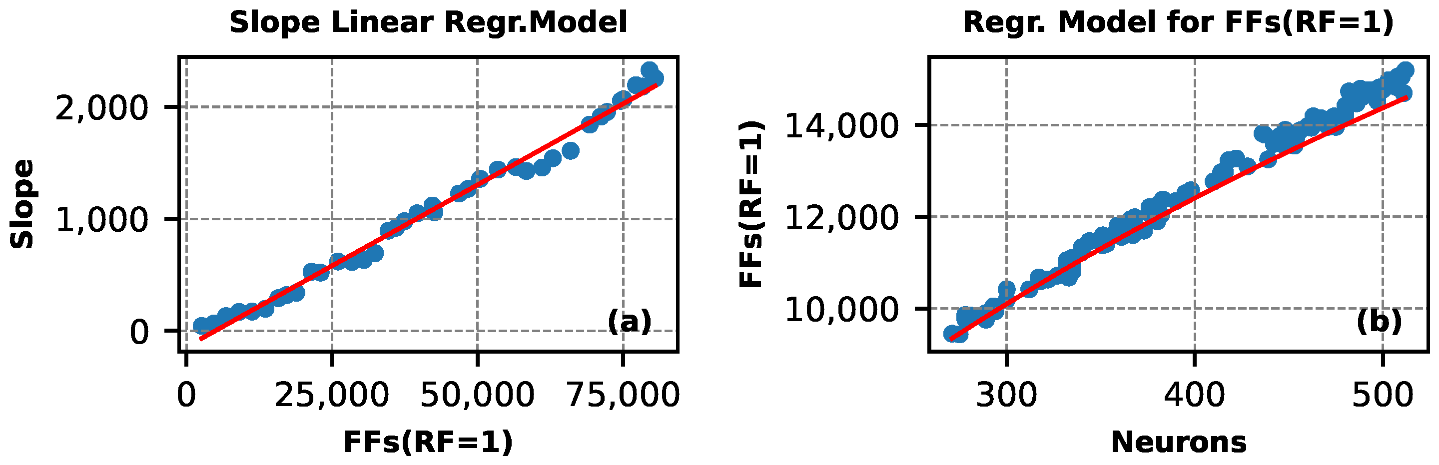
Generic multipliers in DSPs and RF = 1: The number of utilized LUTs can be derived from (1) by removing the ${\mathrm{K}}_1$ term. In this case, the number of DSPs is $\sum {\mathrm{W}}_{\mathrm{gm}}$, where ${\mathrm{W}}_{\mathrm{gm}}$ represents the number of the non-shared weights that require generic multipliers.

Generic multipliers in LUTs and RF > 1: RF > 1 sets the maximum number of the generated generic multipliers equal to $\mathrm{M}=$ ($\mathrm{N}·\mathrm{I}-\mathrm{Zw})/\mathrm{RF}$ [40]. Therefore, the LUTs can be found by (1) with ${\mathrm{K}}_1=\sum \mathrm{LUT}(\mathrm{gen}.\mathrm{mult}.)$ if the number of generated generic multipliers is smaller than $\mathrm{M}$, or ${\mathrm{K}}_1=\mathrm{M}·\mathrm{LUT}(\mathrm{gen}.\mathrm{mult})$ otherwise.

Generic multipliers in DSPs and RF > 1: The number of LUTs are calculated by (1) by removing the K₁ term. The number of the utilized DSPs is W_gm if the number of the generic multipliers is smaller than M or equal to M otherwise.

3.2. FFs Estimator

The number of the utilized FFs depends on the layer’s architecture (i.e., level of parallelism) and its size. HLS registers the outputs of all the multiplications and accumulations to reduce the length of the combinational paths. A design with RF = 1 requires many multipliers; thus, more registers are needed to temporarily store the outputs of each multiplier. On the other hand, when RF > 1, it reduces the number of unique generic multipliers, thereby decreasing the number of FFs. However, it also increases the depth of the pipeline and thus the required FFs for control and dataflow.

The relationship between the RF and the number of required FFs for layers of different sizes is presented in Figure 3. We generated 40 random dense layers at 300 MHz on the PYNQ-Z2 platform with 8-bit coefficients and a number of neurons and inputs in the [20, 512] range. Each layer was synthesized 20 times with RF values from 1 to 20. Every curve in Figure 3 represents one of the 40 layers. Layers with more coefficients utilize more FFs, but as the RF increases, the number of utilized FFs drops due to the decrease in the number of generic multipliers. However, for RF > 7, the number of FFs saturate, s as the registers used to pipeline the layer counterbalance the previous decrease.

Estimating the FFs for RF = 1: To achieve this, we trained a polynomial regression model to estimate the required FFs given the number of the layer’s neurons ($\mathrm{N}$).

We synthesized 400 random dense layers with 8-bit coefficients, where the number of neurons ranged from 2 to 512, and the number of inputs $\left(I\right)$ was set constant at 2. Using 250 random points from this dataset, we trained the polynomial regression model and evaluated its estimation accuracy on the remaining 150 points. A first degree polynomial model achieved ${\mathrm{R}}^2=0.94$, a second degree polynomial ${\mathrm{R}}^2=0.93$, and a third degree polynomial ${\mathrm{R}}^2=0.97$; therefore, the third degree polynomial regression model was selected. The relationship between the layer’s number of neurons when I = 2 and the utilized FFs when RF = 1, as well as the fitting of the third degree regression model in this dataset is presented in Figure 4a. As shown in this figure, more neurons generate more bespoke multipliers, leading to the creation of registers at their output.

The number of inputs has a similar effect on the number of bespoke multipliers and hence registers. In this case, the relationship of $\mathrm{I}$ and FFs is perfectly linear, as shown in Figure 5. Therefore, we estimated the number of a layer’s FFs when $\mathrm{RF}=1$ by

$$\begin{array}{c}\mathrm{FFs}(\mathrm{RF}=1)={\displaystyle \frac{\mathrm{I}}{2}}·\mathrm{PR}\left(\mathrm{N}\right),\end{array}$$

(2)

where $\mathrm{PR}\left(\mathrm{N}\right)$ denotes the polynomial regression model.

Estimating the FFs for RF > 1: We used a linear approximation to estimate the decrease in the FFs when RF increases from 1 to 7 (see Figure 3). To obtain the slope of these linear approximations given the FFs(RF = 1), we trained a linear regression model. Figure 4b shows the slope of 50 linear approximations for different FFs(RF = 1), indicating that higher FFs(RF = 1) values correspond to steeper slopes. This observation is also evident in Figure 3.

To obtain the slope estimates, we employed a dataset of 150 random layers with 8-bit coefficients, synthesized at a 300 MHz target clock frequency on the PYNQ-Z2 platform. We trained a linear regression model on 100 points and evaluated its accuracy on 50 points. The achieved ${\mathrm{R}}^2$ value was 0.98. Therefore, a layer’s FFs number can be estimated by

$$\begin{array}{c}\mathrm{Slope}=\mathrm{FFs}(\mathrm{RF}=1)·c_0-c_1\end{array}$$

(3)

$$\begin{array}{c}\mathrm{FFs}=\mathrm{FFs}(\mathrm{RF}=1)-\mathrm{Slope}·\min (\mathrm{RF},7),\end{array}$$

(4)

where ${\mathrm{c}}_0=0.0028$ and ${\mathrm{c}}_1=143$ are the trained coefficients of the slope’s linear regression model.

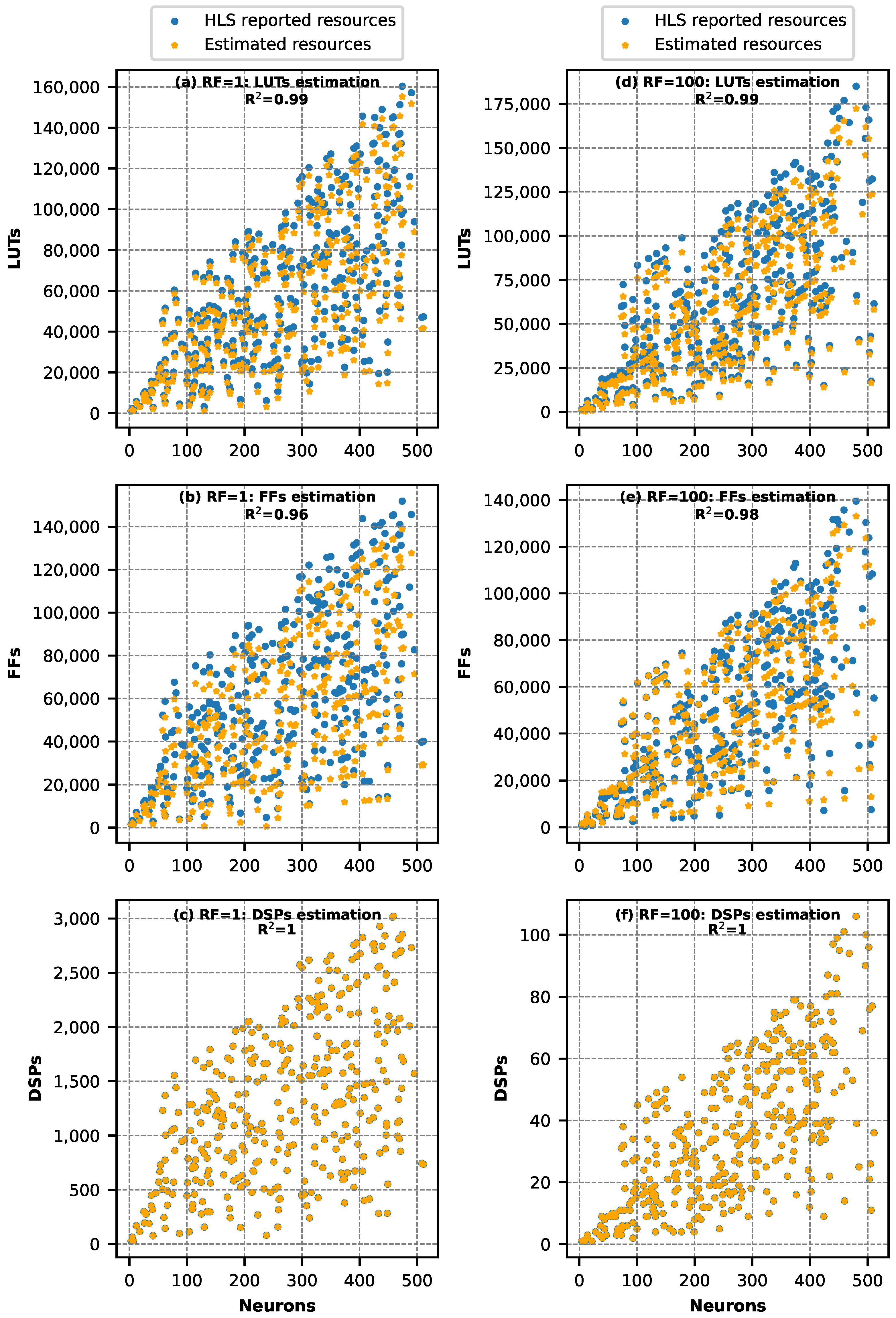
4. Experimental Analysis

Our resource estimator was evaluated on MLPs designed with six different architectures using hls4ml. Specifically, those architectures were dense layers designed with $\mathrm{RF}$ 1, 2, and 100, and for the generic multipliers, either LUT or DSP implementation was selected.

In all the evaluations, the target device was the PYNQ-Z2 with a 300 MHz clock frequency, and all the designs had positive slack.

First, we evaluated the efficacy of our estimator in predicting the resources required by only one dense layer. For the considered architectures, we performed Monte-Carlo simulations with 400 randomly generated dense layers by hls4ml. Specifically, the number of neurons and layer’s inputs were uniformly sampled in the range [2, 512], while random 8-bit coefficients were generated for the neurons. Figure 6 presents the Monte-Carlo results when the generic multipliers were implemented in LUTs, and thus no DSPs were used. The average relative root-mean square error (RRMSE) for the LUT estimation was $0.82\%$ and $1.81\%$ for the FFs, in these examined architectures. In all cases, the ${\mathrm{R}}^2$ was above 0.95. Hence, our estimator can relatively accurately predict the required FFs and LUTs. Similarly, scatter plots in Figure 7 present the same analysis when the generic multipliers were implemented in DSPs. In Figure 7, $\mathrm{RF}=1$ and 100 are shown. In this case, the number of utilized DSPs (Figure 7c,f) were precisely estimated (i.e., zero error) for all the layers and both architectures. Again, in Figure 7, the LUTs and FFs are relatively accurately predicted with ${\mathrm{R}}^2$ being higher than 0.96. For $\mathrm{RF}=2$, similar results to $\mathrm{RF}=1$ were obtained (i.e, ${\mathrm{R}}^2=0.99$$,{\mathrm{R}}^2=0.97$, and ${\mathrm{R}}^2=1$ for the LUTs’, FFs’, and DSPs’ estimation, respectively,) and thus are not presented in Figure 7 for readability reasons. The average RRMSE for this type of implementation when RF = 1, 2, 100 was $1.57\%$ for the LUT estimation and $1.79\%$ for the FF estimation, respectively.

Next, we assessed the efficiency of our estimator in predicting the resource utilization of five MLPs commonly considered in the TinyML domain [11].

These MLPs were designed with all the aforementioned architectures. The examined MLPs were jet-tagging, which is the typical benchmark of hls4ml; human activity recognition (HAR) using smartphones [40]; breast cancer and arrhythmia [41], common classification MLPs on small FPGAs [12]; and the typically used image classification with a 14 × 14 pixels MNIST dataset. The HLS synthesis of the examined MLPs was performed using Vitis 2022.1 HLS on a server with single-threaded execution, with an Intel(R) Xeon(R) Gold 5218R CPU @ 2.10 GHz and 252 GB of RAM. The topology, inference accuracy, the time required by HLS to estimate the resource utilization for these MLPs, and the time that was required by our estimator are all reported in

Table 1. Evaluated MLPs.

Dataset	${\mathbf{A}}^{ \mathbf{★}}$	${\mathbf{T}}^{ †}$	HLS *	Ours *
Jet-tagging	0.76	(16, 64, 32, 32, 5)	480 s	0.03 s
HAR	0.95	(561, 20, 64, 64, 6)	13,800 s	0.147 s
MNIST (14 × 14)	0.97	(192, 56, 64, 32, 10)	3360 s	0.11 s
Breast cancer	0.99	(10, 5, 3, 2)	60 s	0.018 s
Arrhythmia	0.62	(274, 8, 16)	360 s	0.022 s

$★$ Inference accuracy using 8-bit coefficients and inputs. † The MLPs topology (input, hidden layers, output). * Single-threaded execution on Intel Xeon5218R.

.

The barplots in Figure 8 present our resource estimation as well as the resources reported by HLS for the examined MLPs. In Figure 8, the generic multipliers are implemented in LUTs, while all three $\mathrm{RF}$ values are explored. As shown, our estimator can relatively accurately predict the FFs and LUTs. Specifically, the obtained ${\mathrm{R}}^2$ across all the explored MLP-$\mathrm{RF}$ combinations was 0.97 and 0.96 for the LUTs and FFs, respectively. The smallest MLP (breast cancer) exhibited the least accurate estimation. For breast cancer, the $\mathrm{RRMSE}$ was 27% and 14% for the LUTs and FFs, respectively. The latter is explained by the fact that in such small MLPs, the resources required for the ReLU and the Softmax activation layers that are used are considerable with respect to the resources needed by the dense layers. However, the resources utilized by the activation layers were minimal and thus negligible for quite larger networks, not impacting our estimation accuracy.

The barplots in Figure 9 present the same analysis when the generic multipliers are implemented on the DSPs. As shown, the number of DSPs can be precisely predicted for all cases. Again, high estimation accuracy was obtained. In this evaluation, the ${\mathrm{R}}^2$ over all MLP-$\mathrm{RF}$ pairs was 0.97.

Finally, it is noted that the execution time of our estimator did not exceed 147 ms on a single-threaded execution on Intel Xeon5218R. As shown in Table 1, HLS requires from 1 min up to 230 min to generate the respective report.

5. Conclusions

FPGAs constitute promising devices for deploying TinyML applications since they deliver high energy efficiency and low latency. A fast estimation of the design’s feasibility/cost is crucial to avoid time-consuming design iterations and to enable hardware-aware high-level model optimizations. In this paper, we propose the first resource estimator for bespoke MLPs built upon the state-of-the-art hls4ml. Our estimator attains relatively accurate resource estimation in less than 147 $\mathrm{ms}$.

References

1. Prakash, S.; Callahan, T.; Bushagour, J.; Banbury, C.; Green, A.V.; Warden, P.; Ansell, T.; Reddi, V.J. CFU Playground: Full-Stack Open-Source Framework for Tiny Machine Learning (tinyML) Acceleration on FPGAs. arXiv 2022, arXiv:2201.01863. [Google Scholar]
2. Ray, P. A review on TinyML: State-of-the-art and prospects. J. King Saud-Univ.-Comput. Inf. Sci. 2022, 34, 1595–1623. [Google Scholar] [CrossRef]
3. Kok, C.; Siek, L. Designing a Twin Frequency Control DC-DC Buck Converter Using Accurate Load Current Sensing Technique. Electronics 2024, 13, 45. [Google Scholar] [CrossRef]
4. Makni, M.; Baklouti, M.; Niar, S.; Abid, M. Hardware resource estimation for heterogeneous FPGA-based SoCs. In Proceedings of the Symposium on Applied Computing, Marrakech, Morocco, 4–6 April 2017; pp. 1481–1487. [Google Scholar]
5. Fahim, F.; Hawks, B.; Herwig, C.; Hirschauer, J.; Jindariani, S.; Tran, N.; Carloni, L.P.; Di Guglielmo, G.; Harris, P.; Krupa, J.; et al. hls4ml: An Open-Source Codesign Workflow to Empower Scientific Low-Power Machine Learning Devices. arXiv 2021, arXiv:2103.05579. [Google Scholar]
6. Umuroglu, Y.; Fraser, N.J.; Gambardella, G.; Blott, M.; Leong, P.; Jahre, M.; Vissers, K. FINN: A Framework for Fast, Scalable Binarized Neural Network Inference. arXiv 2016, arXiv:1612.07119. [Google Scholar]
7. Ngadiuba, J.; Loncar, V.; Pierini, M.; Summers, S.; Di Guglielmo, G.; Duarte, J.; Harris, P.; Rankin, D.; Jindariani, S.; Liu, M.; et al. Compressing deep neural networks on FPGAs to binary and ternary precision with HLS4ML. Mach. Learn. Sci. Technol. 2021, 2, 015001. [Google Scholar] [CrossRef]
8. Meng, J.; Venkataramanaiah, S.K.; Zhou, C.; Hansen, P.; Whatmough, P.; Seo, J.S. FixyFPGA: Efficient FPGA Accelerator for Deep Neural Networks with High Element-Wise Sparsity and without External Memory Access. In Proceedings of the Conference on Field-Programmable Logic and Applications, Dresden, Germany, 30 August–3 September 2021. [Google Scholar]
9. Borras, H.; Di Guglielmo, G.; Duarte, J.; Ghielmetti, N.; Hawks, B.; Hauck, S.; Hsu, S.C.; Kastner, R.; Liang, J.; Meza, A.; et al. Open-source FPGA-ML codesign for the MLPerf Tiny Benchmark. arXiv 2022, arXiv:2206.11791. [Google Scholar]
10. Kallimani, R.; Pai, K.; Raghuwanshi, P.; Iyer, S.; Onel, L. TinyML: Tools, Applications, Challenges, and Future Research Directions. arXiv 2023, arXiv:2303.13569. [Google Scholar] [CrossRef]
11. Rajapakse, V.; Karunanayake, I.; Ahmed, N. Intelligence at the Extreme Edge: A Survey on Reformable TinyML. ACM Comput. Surv. 2023, 55, 1–30. [Google Scholar] [CrossRef]
12. Chen, C.; da Silva, B.; Yang, C.; Ma, C.; Li, J.; Liu, C. AutoMLP: A Framework for the Acceleration of Multi-Layer Perceptron Models on FPGAs for Real-Time Atrial Fibrillation Disease Detection. IEEE Trans. Biomed. Circuits Syst. 2023, 17, 1371–1386. [Google Scholar] [CrossRef]
13. Zhang, X.; Jiang, W.; Shi, Y.; Hu, J. When Neural Architecture Search Meets Hardware Implementation: From Hardware Awareness to Co-Design. In Proceedings of the IEEE Computer Society Annual Symposium on VLSI (ISVLSI), Miami, FL, USA, 15–17 July 2019. [Google Scholar]
14. Reddi, V.J.; Plancher, B.; Kennedy, S.; Moroney, L.; Warden, P.; Agarwal, A.; Banbury, C.; Banzi, M.; Bennett, M.; Brown, B.; et al. Widening Access to Applied Machine Learning with TinyML. arXiv 2021, arXiv:2106.04008. [Google Scholar]
15. Sanchez-Iborra, R.; Skarmeta, A.F. TinyML-Enabled Frugal Smart Objects: Challenges and Opportunities. IEEE Circuits Syst. Mag. 2020, 20, 4–18. [Google Scholar] [CrossRef]
16. TinyML. Available online: https://github.com/tinyMLx/courseware/tree/master/edX (accessed on 1 December 2024).
17. Zhai, X.; Si, A.; Amira, A.; Bensaali, F. MLP Neural Network Based Gas Classification System on Zynq SoC. IEEE Access 2016, 4, 8138–8146. [Google Scholar] [CrossRef]
18. Coelho, C.N.; Kuusela, A.; Li, S.; Zhuang, H.; Ngadiuba, J.; Aarrestad, T.K.; Loncar, V.; Pierini, M.; Pol, A.A.; Summers, S. Automatic heterogeneous quantization of deep neural networks for low-latency inference on the edge for particle detectors. arXiv 2020, arXiv:2006.10159. [Google Scholar] [CrossRef]
19. Campos, J.; Mitrevski, J.; Tran, N.; Dong, Z.; Gholaminejad, A.; Mahoney, M.W.; Duarte, J. End-to-end codesign of Hessian-aware quantized neural networks for FPGAs. ACM Trans. Reconfig. Technol. Syst. 2023, 17, 1–22. [Google Scholar] [CrossRef]
20. Banbury, C.; Reddi, V.J.; Torelli, P.; Holleman, J.; Jeffries, N.; Kiraly, C.; Montino, P.; Kanter, D.; Ahmed, S.; Pau, D.; et al. MLPerf Tiny Benchmark. arXiv 2021, arXiv:2106.07597. [Google Scholar]
21. Hui, H.; Siebert, J. TinyML: A Systematic Review and Synthesis of Existing Research. In Proceedings of the IEEE, International Conference on Artificial Intelligence in Information and Communication (ICAIIC), Jeju Island, Republic of Korea, 21–24 February 2022. [Google Scholar]
22. Wang, Y.; Xu, J.; Han, Y.; Li, H.; Li, X. DeepBurning: Automatic generation of FPGA-based learning accelerators for the neural network family. In Proceedings of the 53rd Annual Design Automation Conference, Austin, TX, USA, 5–9 June 2016; Volume 1. [Google Scholar]
23. Zhao, Y.; Gao, X.; Guo, X.; Liu, J.; Wang, E.; Mullins, R.; Cheung, P.Y.; Constantinides, G.; Xu, C.Z. Automatic Generation of Multi-Precision Multi-Arithmetic CNN Accelerators for FPGAs. In Proceedings of the IEEE, International Conference on Field-Programmable Technology (ICFPT), Tianjin, China, 9–13 December 2019. [Google Scholar]
24. Ye, H.; Zhang, X.; Huang, Z.; Chen, G.; Deming, C. HybridDNN: A framework for high-performance hybrid DNN accelerator design and implementation. In Proceedings of the 57th ACM/EDAC/IEEE Design Automation Conference, San Francisco, CA, USA, 20–24 July 2020. [Google Scholar]
25. Jahanshahi, A.; Sharifi, R.; Rezvani, M.; Zamani, H. Inf4Edge: Automatic Resource-aware Generation of Energy-efficient CNN Inference Accelerator for Edge Embedded FPGAs. In Proceedings of the IEEE, 12th International Green and Sustainable Computing Conference (IGSC), Pullman, WA, USA, 18–21 October 2021. [Google Scholar]
26. Ng, W.; Goh, W.; Gao, Y. High Accuracy and Low Latency Mixed Precision Neural Network Acceleration for TinyML Applications on Resource-Constrained FPGAs. In Proceedings of the IEEE International Symposium on Circuits and Systems (ISCAS), Singapore, 19–22 May 2024; Volume 1. [Google Scholar]
27. Khalil, K.; Mohaidat, T.; Darwich, M.D.; Kumar, A.; Bayoumi, M. Efficient Hardware Implementation of Artificial Neural Networks on FPGA. In Proceedings of the IEEE 6th International Conference on AI Circuits and Systems (AICAS), Abu Dhabi, United Arab Emirates, 22–25 April 2024. [Google Scholar]
28. Whatmough, P.; Zhou, C.; Hansen, P.; Venkataramanaiah, S.; Sun, S.; Mattina, M. FixyNN: Efficient Hardware for Mobile Computer Vision via Transfer Learning. arXiv 2019, arXiv:1902.11128. [Google Scholar]
29. Jiménez-González, D.; Alvarez, C.; Filgueras, A.; Martorell, X.; Langer, J.; Noguera, J.; Vissers, K. Coarse-Grain Performance Estimator for Heterogeneous Parallel Computing Architectures like Zynq All-Programmable SoC. arXiv 2015, arXiv:1508.06830. [Google Scholar]
30. Zhong, G.; Prakash, A.; Liang, Y.; Mitra, T.; Niar, S. Lin-Analyzer: A high-level performance analysis tool for FPGA-based accelerators. In Proceedings of the 53nd ACM/EDAC/IEEE Design Automation Conference (DAC), Austin, TX, USA, 5–9 June 2016. [Google Scholar]
31. Dai, S.; Zhou, Y.; Zhang, H.; Ustun, E.; Young, E.F.; Zhang, Z. Fast and Accurate Estimation of Quality of Results in High-Level Synthesis with Machine Learning. In Proceedings of the Annual International Symposium on Field-Programmable Custom Computing Machines (FCCM), Boulder, CO, USA, 29 April–1 May 2018. [Google Scholar]
32. Makrani, H.M.; Sayadi, H.; Dinakarrao, S.; Homayoun, H. Pyramid: Machine Learning Framework to Estimate the Optimal Timing and Resource Usage of a High-Level Synthesis Design. In Proceedings of the 29th International Conference on Field Programmable Logic and Applications (FPL), Barcelona, Spain, 9–13 September 2019. [Google Scholar]
33. Choi, Y.k.; Cong, J. HLS-Based Optimization and Design Space Exploration for Applications with Variable Loop Bounds. In Proceedings of the IEEE/ACM International Conference on Computer-Aided Design (ICCAD), San Diego, CA, USA, 5–8 November 2018. [Google Scholar]
34. Li, P.; Zhang, P.; Pouchet, L.; Cong, J. Resource-Aware Throughput Optimization for High-Level Synthesis. In Proceedings of the 2015 ACM/SIGDA International Symposium on Field-Programmable Gate Arrays, Monterey, CA, USA, 22–24 February 2015; Volume 1. [Google Scholar]
35. Li, B.; Zhang, X.; You, H.; Qi, Z.; Zhang, Y. Machine Learning Based Framework for Fast Resource Estimation of RTL Designs Targeting FPGAs. ACM Trans. Des. Autom. Electron. Syst. 2022, 28, 1–16. [Google Scholar] [CrossRef]
36. Schumacher, P.; Jha, P. Fast and accurate resource estimation of RTL-based designs targeting FPGAS. In Proceedings of the International Conference on Field Programmable Logic and Applications, Milano, Italy, 31 August–2 September 2008. [Google Scholar]
37. Prost-Boucle, A.; Muller, O.; Rousseau, F. A Fast and Autonomous HLS Methodology for Hardware Accelerator Generation under Resource Constraints. In Proceedings of the IEEE, Euromicro Conference on Digital System Design, Los Alamitos, CA, USA, 4–6 September 2013. [Google Scholar]
38. Adam, M.; Frühauf, H.; Kókai, G. Quick Estimation of Resources of FPGAs and ASICs Using Neural Networks. In Proceedings of the Lernen, Wissensentdeckung und Adaptivität (LWA) 2005, GI Workshops, Saarbrücken, Germany, 10–12 October 2005; Volume 1, pp. 210–215. [Google Scholar]
39. Ullrich, K.; Meeds, E.; Welling, M. Soft Weight-Sharing for Neural Network Compression. In Proceedings of the International Conference on Learning Representations (ICLR), San Juan, Puerto Rico, 2–4 May 2016; Volume 1. [Google Scholar]
40. Duarte, J.; Han, S.; Harris, P.; Jindariani, S.; Kreinar, E.; Kreis, B.; Ngadiuba, J.; Pierini, M.; Rivera, R.; Tran, N.; et al. Fast inference of deep neural networks in FPGAs for particle physics. J. Instrum. 2018, 13, P07027. [Google Scholar] [CrossRef]
41. Dua, D.; Graff, C. UCI Machine Learning Repository. 2017. Available online: http://archive.ics.uci.edu/ml (accessed on 1 December 2024).
Figure 1. LUT utilization of bespoke multiplications on ZYNQ-7000 devices: I is an 8-bit value, and w is a constant value in [ 128 , 127 ] .
Electronics 14 00247 g001
Figure 2. Example of bespoke multiplications of two neurons with two inputs when: (a) an RF = 2, and (b) weight sharing results in multiplication sharing.
Electronics 14 00247 g002
Figure 3. Synthesis of 40 dense layers with 8-bit coefficients and random size in the [20, 512] range. Each layer is synthesized 20 times for RF [ 1 , 20 ] . Each line represents one of the 40 random dense layers and shows the FFs utilization after synthesizing each layer 20 times for the examined RF values.
Electronics 14 00247 g003
Figure 4. (a) The third degree polynomial regression model to estimate the FFs utilization when RF = 1 and the number of the layer’s inputs is fixed to I = 2 and (b) the linear regression model used to estimate the slopes of the linear approximations of the FFs utilization beteween the RF = 1 and RF = 7 points.
Electronics 14 00247 g004
Figure 5. FFs utilization when RF = 1 for 40 fully connected layers with random 8-bit coefficients when the number of the layers neurons is fixed to 100 and the number of the layer’s inputs ranges from 2 to 40.
Electronics 14 00247 g005
Figure 6. LUTs’ and FFs’ estimation from a 400 point Monte-Carlo simulation. The layer’s generic multipliers are implemented in LUTs. (a) LUTs’ estimation when RF = 1 , (b) FFs’ estimation when RF = 1 , (c) LUTs’ estimation when RF = 2 , (d) FFs’ estimation when RF = 2 , (e) LUTs’ estimation when RF = 100 , (f) FFs’ estimation when RF = 100 .
Electronics 14 00247 g006
Figure 7. LUTs’, FFs’, and DSPs’ estimation from a 400 point Monte-Carlo simulatio. The layer’s generic multipliers are implemented in DSPs. (a) LUTs’ estimation when RF = 1 , (b) FFs’ estimation when RF = 1 , (c) DSPs’ estimation when RF = 1 , (d) LUTs’ estimation when RF = 100 , (e) FFs’ estimation when RF = 100 , (f) DSPs’ estimation when RF = 100 .
Electronics 14 00247 g007
Figure 8. Comparison between our estimator and HLS for the LUTs’ and FFs’ utilization for the 5 MLPs. The generic multipliers are implemented in LUTs. Each figure shows the utilized resourced when (a) RF = 1 , (b) RF = 2 , and (c) RF = 100 . The Y-axis is in logarithmic scale.
Electronics 14 00247 g008
Figure 9. Comparison between our estimator and HLS for the LUTs’, FFs’, and DSPs’ utilization for the five MLPs. The generic multipliers are implemented in DSPs. Each figure shows the utilized resourced when (a) RF = 1 , (b) RF = 2 , and (c) RF = 100 . The Y-axis is in logarithmic scale.
Electronics 14 00247 g009