Large Language Model-Based Tuning Assistant for Variable Speed PMSM Drive with Cascade Control Structure

Abstract

A cascade control structure (CCS) is still the most commonly used control scheme in variable speed control (VSC) electrical drives with alternating current (AC) motors. Several tuning methods are used to select the coefficients of controllers applied in CCS. These approaches can be divided into analytical, empirical, and heuristic ones. Regardless of the tuning method used, there is still a question of whether the CCS is tuned optimally in terms of considered performance indicators to provide high-performance behavior of the electrical drive. Recently, artificial intelligence-based methods, e.g., swarm-based metaheuristic algorithms (SBMAs), have been extensively examined in this field, giving promising results. Moreover, the intensive development of artificial intelligence (AI) assistants based on large language models (LLMs) supporting decision-making processes is observed. Therefore, it is worth examining the ability of LLMs to tune the CCS in the VSC electrical drive. This paper investigates tuning methods for the cascade control structure equipped with PI-type current and angular velocity controllers for PMSM drive. Sets of CCS parameters from electrical engineers with different experiences are compared with reference solutions obtained by using the SBMA approach and LLMs. The novel LLM-based Tuning Assistant (TA) is developed and trained to improve the quality of responses. Obtained results are assessed regarding the drive performance, number of attempts, and time required to accomplish the considered task. A quantitative analysis of LLM-based solutions is also presented. The results indicate that AI-based tuning methods and the properly trained Tuning Assistant can significantly improve the performance of VSC electrical drives, while state-of-the-art LLMs do not guarantee high-performance drive operation.

1. Introduction

Variable speed drives (VSDs) with permanent magnet synchronous motors are commonly applied in high-performance industry applications such as robotics, Computerized Numerical Control (CNC) machines, and recently in electromobility and aircraft [1,2,3,4,5,6]. It is caused by superior dynamic properties, reliability, and energy efficiency of considered motors [7,8,9]. Full use of the listed features requires precise information about drive signals and an accurate control scheme. The actual values of the motor’s phase currents and the shaft angular position can be obtained using encoders and Hall-effect current sensors. To improve the VSD level of safety, estimation techniques and fault detection mechanisms are introduced [10,11,12,13,14]. The electromagnetic torque in PMSM with surface-mounted magnets depends on the q-axis current. Therefore, current ripples will produce a pulsating torque responsible for noise and vibrations of the drive [15,16]. Current ripples are caused by measurement errors (offset and scaling errors), the dead-time effect, inaccuracies in motor manufacturing, and cogging phenomena [15,17]. As shown in [15], both the control structure and the parameters of controllers also affect the current waveforms. Due to this, secondary control objectives considering current ripples should be introduced during the control scheme selection and/or tuning of the controllers to provide high-performance operation of the drive.

PMSM, as a typical AC motor, is described by electrical and mechanical equations with different dynamic properties. Therefore, control schemes can be divided into two main groups: (i) cascade control structure (CCS) with the inner and the outer control loops, and (ii) cascade-free with a complex control scheme. The second approach, implemented as a state feedback control, provides robustness against parameter variations and better disturbance compensation compared to CCS [8,15,18]. However, its tuning process is relatively complex and usually requires expert knowledge. Recently, SBMA has been applied in this field, and these show superior properties in comparison to the analytical approach [15,18]. It should be pointed out that SBMA is based on the optimization of the performance function, and the overall drive performance is strongly related to its components. Therefore, expert knowledge and experience are required during the performance function construction and SBMA parameter selection [19,20].

Contrary to the cascade-free complex control scheme, the CCS is based on a series of connections of well-known PID controllers. In this approach, controllers are tuned separately, and several tuning methods can be used. These can be divided into three main groups: (i) empirical, (ii) analytical, and (iii) computer-aided. In the first group, the controller coefficients are usually selected by trial and error or using Ziegler–Nichols-like approaches. The overall drive performance and the time needed to accomplish the tuning procedure are strongly related to user experience and may result in non-optimal behavior [21,22]. From the literature review, it can be seen that mistakes that disable correct drive operation are common, even for a basic control structure. In [23], negative values of the PI speed controller are enabled, which may result in positive feedback and loss of stability. From the results shown in [24], one can see that improper controller tuning may result in a huge overshoot and poor load torque compensation. Instead of applying a proper tuning procedure, the authors suggest the introduction of low-pass filters or non-linear control.

The analytical approach utilizes a symmetric optimum criterion for the angular velocity controller and a magnitude optimum criterion or an internal model control (IMC) theory for the current controller [25,26]. These approaches require more advanced knowledge from electrical drives and control theory compared to the empirical solutions listed above and, therefore, are commonly applied by more advanced electrical engineers. In [27], the IMC is combined with model following control to provide velocity control of PMSM with reduced impact of the load torque. The authors report that the presented control structure is much more insensitive to disturbances at the plant input compared to the classical cascade control structure. On the other hand, an explicit tuning procedure for the controller, which generates an additional control signal responsible for load torque compensation, is not precisely defined. It was also mentioned that the proposed solution is based on model knowledge, and modeling a complex plant, e.g., a CNC control system, can be a challenging task. An optimized PI tuning scheme based on an analytical approach, namely deadbeat predictive conception, is proposed in [28]. It was found that the integration gains in both controllers are equal to zero, and therefore, the load torque observer must be applied to provide steady-state error-free operation of the drive. The formulas proposed for proportional gains of both controllers are simpler compared to the reference solutions but in the angular velocity controller, a manually selected coefficient is present. As the authors reported, its value should be chosen during experimental tests.

As in the case of complex control schemes, the tuning process of PI controllers in a cascade control structure can also be supported by AI-based approaches. In [19,20], several SBMAs are applied to adjust the parameters of the velocity PI controller in the PMSM drive. The objective function responsible for setting the maximum overshoot and the rise time and elimination of the steady-state error has been proposed. The weighting factor has also been introduced to shape the dynamic properties of the control system. Based on the simulation results, it was concluded that the velocity controller is tuned properly, and the drive tracks the given trajectories well, including the load torque compensation. A similar conclusion can be found in [29], where a comparison between a conventional PI speed controller tuned by using the Ziegler–Nichols approach and one using the optimization scheme (i.e., multivariable sliding-mode extremum seeking) is shown. Faster attainment of steady-state, reduced overshoot, and enhanced robustness against load torque and parameter variations were reported. However, the user must select additional parameters responsible for the drive’s dynamic behavior and smooth control action. As in the case of a cascade-free control scheme, the final behavior of the drive with SBMA-tuned controllers strongly depends on the performance function applied, and therefore, expert knowledge is required in this area, especially if secondary control objectives (e.g., torque ripple minimization) are considered.

The intensive development of large language models causes their area of application to expand [30]. Recently, the ability of LLMs to solve undergraduate control engineering problems has been examined using the state-of-the-art LLM’s: GPT-4, Claude 3 Opus, and Gemini 1.0 Ultra [31]. It was reported that answers generated by LLMs are sometimes inconsistent even for the same problem, and the reasoning and calculation capabilities must be improved in the future. In [32], the innovative combination of an adaptive PID controller with an LLM to enhance explainability was proposed. The potential of LLMs to bolster the control loop performance has been demonstrated. As an example, the integration of the GPT-3.5-turbo into the control loop of a convoy of autonomous vehicles was shown in a simulation study.

In this paper, a novel Tuning Assistant based on the large language model is proposed and examined. A dataset necessary to accurately train the TA is described, and a two-stage training process is presented. The developed solution is used to find the coefficients of PI-type angular velocity and current controllers for a variable speed drive with a permanent magnet synchronous motor. The obtained results are compared with reference solutions, namely answers from the state-of-the-art LLMs, responses from electrical engineers, and outturns from swarm-based metaheuristic algorithms. A quantitative analysis of the LLM-based solutions is also presented. It is based on the prompt scoring approach and gives information about the accuracy. The innovative use of LLMs in tuning the cascade control structure allows the drive to obtain superior control behavior. To the best of the authors’ knowledge, the developed Tuning Assistant is the first solution available to users and dedicated to tuning controllers for electrical drives.

This paper is organized as follows. Section 2 introduces the mathematical description and methods for the determination of the main parameters of the PMSM. The description of a cascade control structure and tuning methods used in PMSM drives are also included in this section. Section 3 explores the results obtained from the Tuning Assistant. These are compared with reference solutions, namely the state-of-the-art LLMs, swarm-based metaheuristic algorithms, and finally, responses from electrical engineers. In Section 4, the obtained results are discussed. Conclusions and the potential directions for future research are outlined in Section 5.

2. Materials and Methods

2.1. Determination of the Parameters of the PMSM

Analytical methods used to determine coefficients of PI current and velocity controllers are based on the knowledge of the drive’s parameters. These can be obtained using measurements, as shown in [33], or identification described in [34]. In the later part of this section, the calculation of the motor’s electrical and mechanical parameters will be discussed.

2.1.1. Electrical Parameters of the Motor

The electrical part of the PMSM can be described using the following formulas, usually written in $dq$ reference frame:

$$u_d\left(t\right)=L_s{\displaystyle \frac{d{i}_d\left(t\right)}{dt}}+R_s{i}_d\left(t\right)-p{\omega }_m\left(t\right)L_s{i}_q\left(t\right)$$

(1)

$$u_q\left(t\right)=L_s{\displaystyle \frac{d{i}_q\left(t\right)}{dt}}+R_s{i}_q\left(t\right)+p{\omega }_m\left(t\right)L_s{i}_d\left(t\right)+p{\omega }_m\left(t\right){\psi }_f$$

(2)

where $u_d\left(t\right)$, $u_q\left(t\right)$ are space vector components of voltages, $i_d\left(t\right)$, $i_q\left(t\right)$ are current space vector components, ${\omega }_m\left(t\right)$ is angular velocity, $R_s$, $L_s$ are stator resistance and inductance, p is the number of pole pairs, ${\psi }_f$ is flux linkage. From (1)–(2), one can see that precise control of the PMSM currents requires knowledge of the stator resistance and inductance. These can be calculated from the motor’s electrical circuit step response parameters under the assumption that the motor shaft is locked, resulting in elimination of the back-emf components. The motor’s resistance can be computed from the steady-state value of the step response:

$$R_s=u_{ss}/i_{ss}$$

(3)

where $u_{ss}$ is the steady-state value of the commanded voltage, and $i_{ss}$ is the steady-state value of the current, as shown in Figure 1.

Next, the motor’s inductance can be calculated from the obtained time constant:

$$L_s=T_e{R}_s$$

(4)

where $T_e$ is the electrical time constant estimated from the current step response presented above. To improve the accuracy of calculations, the experiment should be conducted for different values of the commanded voltage, and the motor’s shaft should be immobilized. It may also be necessary to take into account the converter gain. In such a case, the steady-state value of the commanded voltage in (1) will be multiplied accordingly [35].

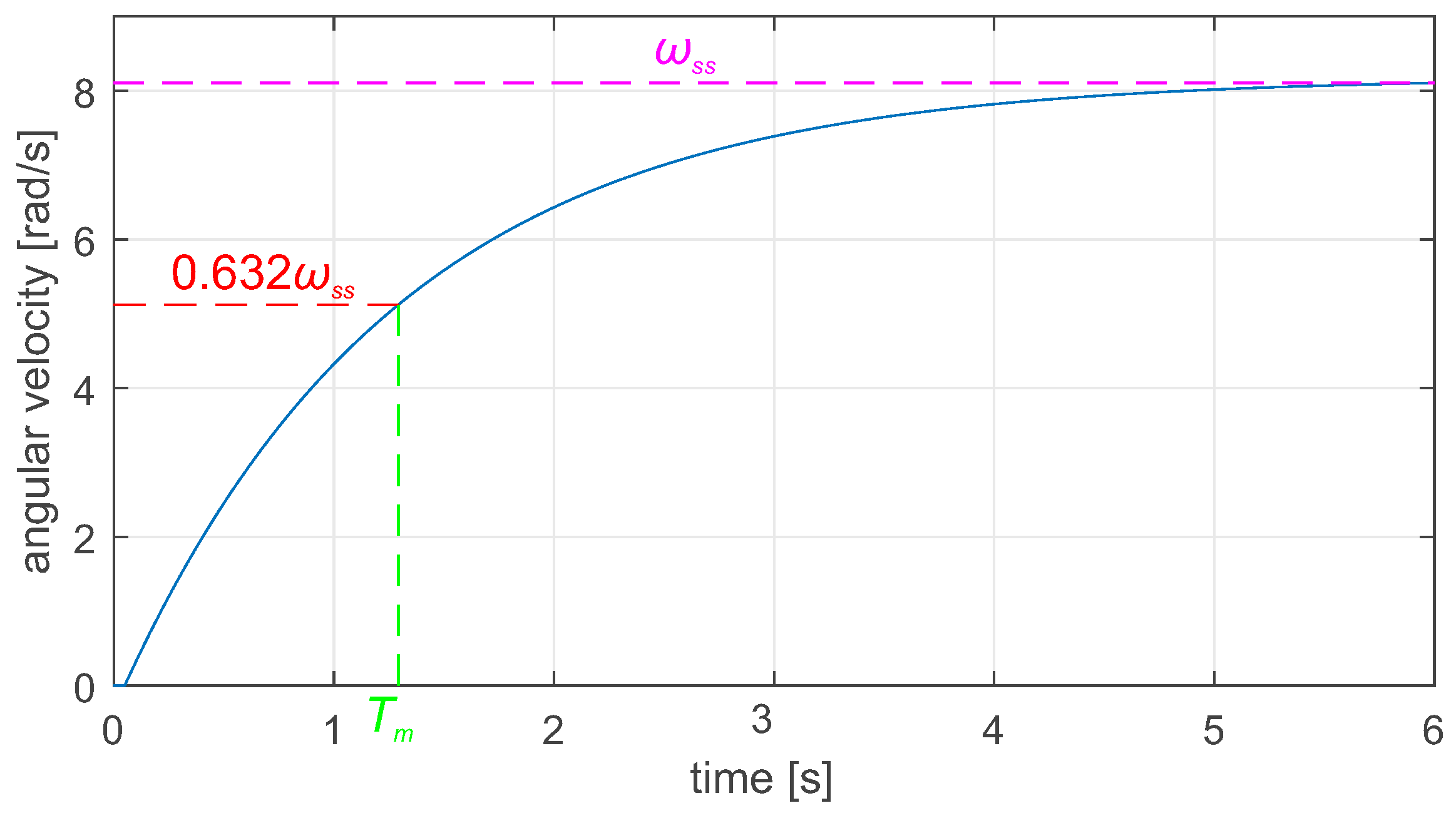
2.1.2. Mechanical Parameters of the Motor

The mechanical part of the PMSM can be described using the following equation:

$$J_m{\displaystyle \frac{d{\omega }_m\left(t\right)}{dt}}=K_t{i}_q\left(t\right)-B_m{\omega }_m\left(t\right)-T_l\left(t\right)$$

(5)

where $J_m$ and $B_m$ are the motor’s moment of inertia and the viscous friction coefficient, $K_t$ is the torque constant, and $T_l\left(t\right)$ is the load torque. From (5), it can be seen that accurate control of the PMSM angular velocity depends on the knowledge of the motor’s mechanical parameters, namely $J_m$, $B_m$, and $K_t$. These can be calculated from the motor’s response parameters if they are unknown. In such a case, it is necessary to command the step values of the reference current and record the angular velocity waveform in the current/torque mode of the drive. The gain coefficient of the mechanical part can be calculated from the following formula:

$$K_m={\displaystyle \frac{{\omega }_{ss}}{i_{ss}{K}_t}}$$

(6)

where ${\omega }_{ss}$ is the steady-state value of the angular velocity. Next, the object’s moment of inertia can be computed from the following formula:

$$J_m={\displaystyle \frac{T_m}{K_m}}$$

(7)

where $T_m$ is the mechanical time constant estimated from the velocity step response, as shown in Figure 2.

Now, it is also possible to estimate the viscous coefficient $B_m$ of the mechanical part of the object using the following formula:

$$B_m=1/K_m$$

(8)

Further information related to the identification of motor parameters can be found in [34].

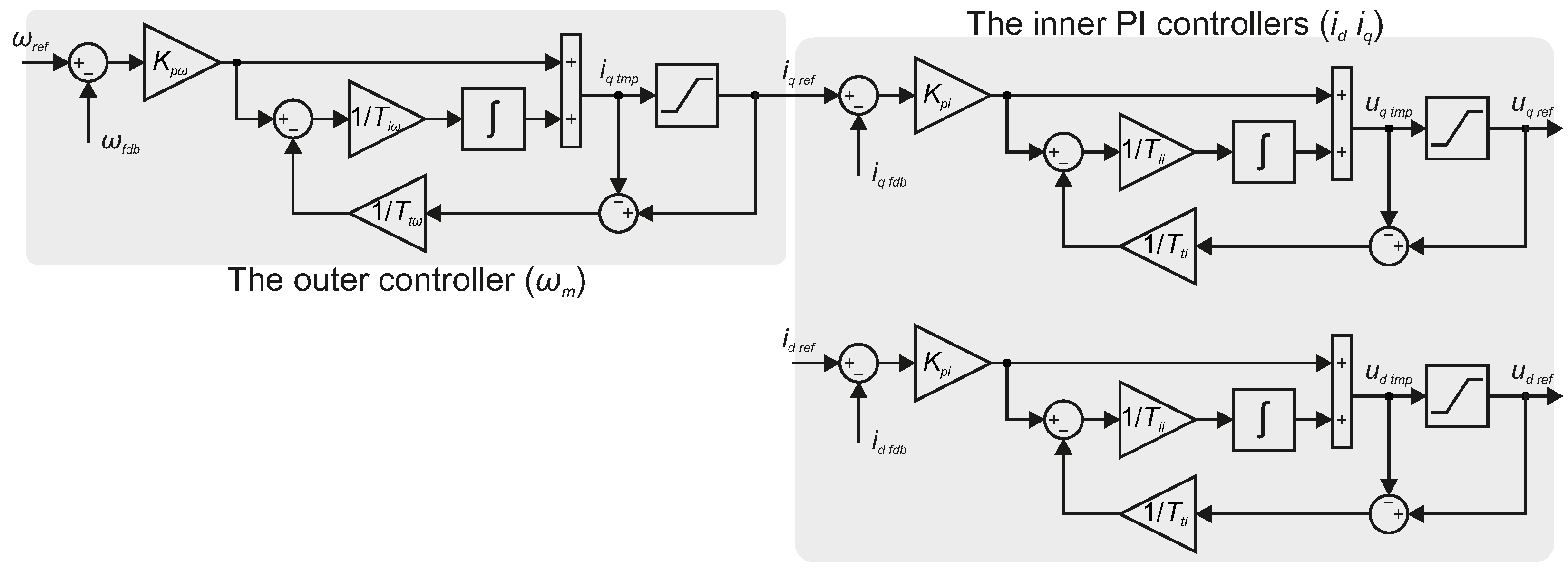
2.2. Cascade Control Structure

As stated before, the cascade control structure (CCS) with the inner and the outer control loops is considered in this study. The choice is related to the behavior of the electrical drive, where different dynamic properties are observed for electrical and mechanical parts, as well as to the well-known structure and tuning methods of PI controllers. The selection procedures of the controller’s coefficients will be discussed in the later part of this section, while the considered CCS is shown in Figure 3.

From Figure 3, it can be seen that a standard or textbook version of the PI controller is utilized. In the case of the outer angular velocity controller, $K_{p\omega }$ is the proportional gain of the controller, while $T_{i\omega }$ is the integration time constant of the controller. Similarly, in the inner current control loop, $K_{pi}$ is the proportional gain of the controller, while $T_{ii}$ is the integration time constant of the controller. The controller from the outer control loop generates a reference signal for the inner control loop, i.e., $i_{qref}$, while the controller from the inner control loop generates a control signal for the modulator [35]. Since nonlinear limitations exist in electrical drives (e.g., limited voltage of the voltage source inverter, limited current, and angular velocity of the PMSM), it may happen that the control variable reaches the actuator limits. In such a case, the error will continue to be integrated by the integral path of the controller, resulting in deterioration of the control performance [36]. To overcome this drawback, the tracking back-calculation method can be implemented to attenuate the integral path during saturation [35]. As shown in Figure 3, the tracking time constants $T_{t\omega }$ and $T_{ti}$ (i.e., anti-windup coefficients) are used in the anti-windup path. These determine how quickly the integral is reset.

In the case of the other controller’s structure, the coefficients should be converted before implementation, as shown in [37]. For example [35], instead of the integration time constant $T_{ix}$, the gain $K_{ix}=1/T_{ix}$ can be utilized. A similar modification can be found for the tracking time constant $T_{tx}$ implemented as the gain $K_{ax}=1/T_{tx}$. Here, the subscript x will be replaced by i for current controllers, while for the angular velocity control loop, it is substituted by $\omega$.

2.3. Tuning Approaches

In this part, the tuning methods of the control structure described previously will be discussed. Typically, these can be divided into two main groups: (i) analytical-based tuning and (ii) empirical-based tuning. Recently, it was found that AI-based approaches can successfully support the tuning process, both analytical- and empirical-based methods. All of these will be discussed later in this section.

2.3.1. Analytical-Based Tuning

In this approach, it is necessary to maintain the tuning order of the controllers, i.e., from the inner (current) to the outer (angular velocity) control loop. In the case of the current control loop tuning, it should first be decided whether the current overshoot is permissible. Since the magnitude optimum criterion presented in [25] provides a fast current response and slight overshoot, these can be used to calculate the controller coefficients analytically. In this case, the dominant time constant in the plant (i.e., $T_e$) is canceled by the zero in the controller, resulting in the following formulas for PI current controller:

$$K_{pi}=L_s{f}_s$$

(9)

$$T_{ii}=L_s/R_s$$

(10)

where $f_s$ is the switching frequency. If the current overshoot is not allowed, the internal model control (IMC) approach presented in [26] can be used to calculate the coefficients of the PI current controller. Here, the parameters of the controller are expressed directly in machine parameters and the desired rise time $t_r$ of the control loop. Such an approach simplifies the design procedure by reducing the trial-and-error steps. According to the IMC approach, the PI current controller’s coefficients will be as follows:

$$K_{pi}=2.2L_s/t_r$$

(11)

$$T_{ii}=L_s/R_s$$

(12)

It is worth pointing out that regardless of the method used, the same formula is proposed for the calculation of the integration time constant. In IMC, a suitable trade-off between the current control loop’s bandwidth and the current signal’s noise can be obtained [35]. The current rise time is typically specified as a couple of control periods [38].

In the next step, the angular velocity controller will be designed. Here, the symmetric optimum criteria can be used [25]. It is necessary to know the object’s moment of inertia, the torque constant of the motor, and the time constant of the current control loop. The PI velocity controller’s coefficients will be as follows:

$$K_{p\omega }={\displaystyle \frac{J_m}{2K_t{T}_{ccl}}}$$

(13)

$$T_{i\omega }=4T_{ccl}$$

(14)

where $T_{ccl}$ is the time constant of the current control loop. As stated in [25], there will be a 43% overshoot if the above-mentioned coefficients are used. To improve the control system’s velocity transient response (i.e., reduction in overshoot), an input filter of reference velocity may be introduced. It is positioned outside the loop without affecting the load torque compensation. As a result, an 8.1% overshoot can be obtained.

The controller’s coefficients obtained using (9)–(10) or (11)–(12) and (13)–(14) should be treated as initial ones. The discretization period from the drive should also be considered during the implementation of the integration time constant. If the control performance needs to be further improved, consider adjusting the anti-windup [36] and/or anti-resonance filters according to the drive documentation. To quickly reset the integrator, a very small value of the tracking time constant $T_t$ should be chosen. As shown in [36], the initial value of this anti-windup coefficient can typically be in the range of $[0.1, 3]$.

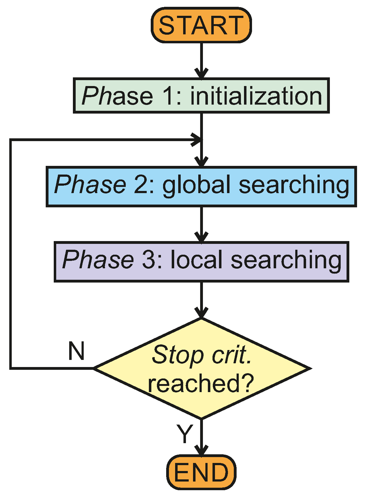
2.3.2. Swarm-Based Tuning

In this approach, computational intelligence is employed to find the optimal coefficients of the controllers. An application of swarm-based metaheuristic algorithms in tuning tasks has recently been observed. It is caused by better convergence and robustness against local minima compared to the exact optimization methods [39]. Contrary to the analytical-based solutions described above, here, all coefficients of the cascade control structure shown in Figure 3 are determined simultaneously. As shown in [39], several SBMAs can be used to solve the tuning task, and the choice may be related to the user experience and/or specific requirements. Regardless of the metaheuristic algorithm used, the general principle of operation can be described by the flowchart shown in Figure 4.

In phase 1, the control parameters specified for an SBMA are set, the population is initialized randomly, and the performance index is calculated for all swarms. Next, a part of the population is employed for global searching for the solution in the defined solution space. The performance index is again calculated for all swarms, and the best solution is remembered. At this stage, the constraint handling method can be employed to abandon solutions that exceed limitations [15]. In phase 3, the rest of the population is sent to the neighborhood of the best solution to improve the result. In order to improve convergence and avoid stagnation in a local minimum, additional mechanisms based on randomly changing the locations of some particles in the solution space can be used [39]. Finally, the optimization process is finished when the condition defined by the stopping criterion is met.

As described before, the operation of SBMAs is based on the optimization of the performance function, and the overall drive performance is strongly related to its components. To provide the desired behavior of the drive, several requirements should be taken into account during the performance index construction. The main control objective for the considered PMSM drive is to assure steady-state error-free operation and good dynamics of the angular velocity for both the reference and the load torque and step changes. Secondary control objectives related to zero d-axis current and chattering-free control signals can also be taken into account if high-performance drive operation is expected. The above-mentioned requirements lead to the construction of the following performance index:

$$J=\underset{0}{\overset{t}{\int }}\alpha {\left({\omega }_m\left(\tau \right)-{\omega }_{ref}\left(\tau \right)\right)}^{2}d\tau +\beta {\left(i_d\left(\tau \right)-i_{dref}\left(\tau \right)\right)}^{2}d\tau +\gamma {\displaystyle \frac{d{u}_q^2}{dt}}$$

(15)

where $\alpha$, $\beta$, and $\gamma$ are the weighting factors responsible for prioritizing the impact of the performance index components. It is also possible to directly control the selected parameters of the plant response (e.g., the rise time, the overshoot) during auto-tuning [19].

In this paper, the ABC optimization method was chosen to find the initial coefficients of the controllers shown in Figure 3. The choice of the ABC is based on the confirmed convergence and repeatability of results obtained in similar tasks [15,18]. The control parameters of the optimization scheme and the results obtained are presented and discussed later in the paper.

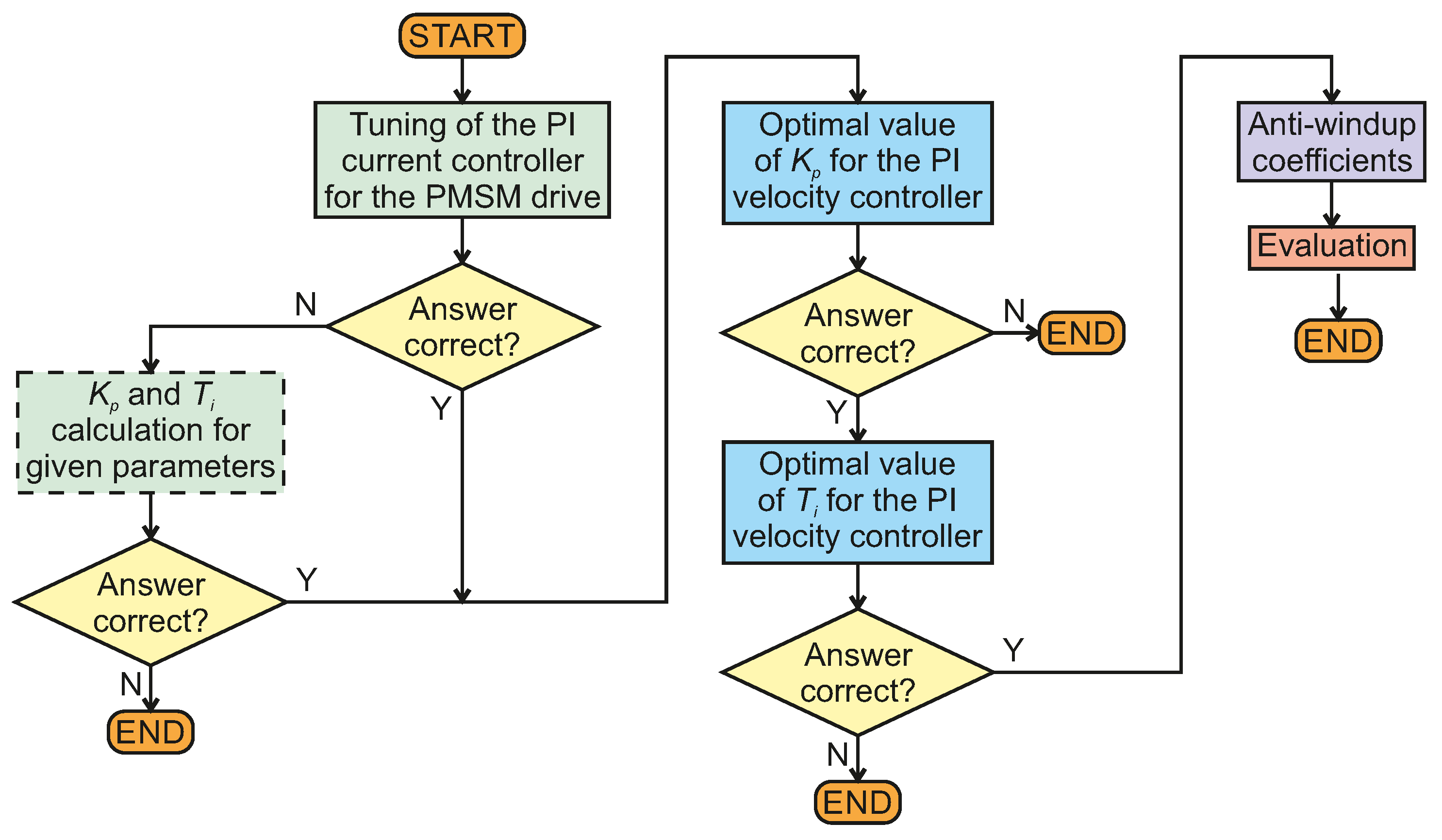
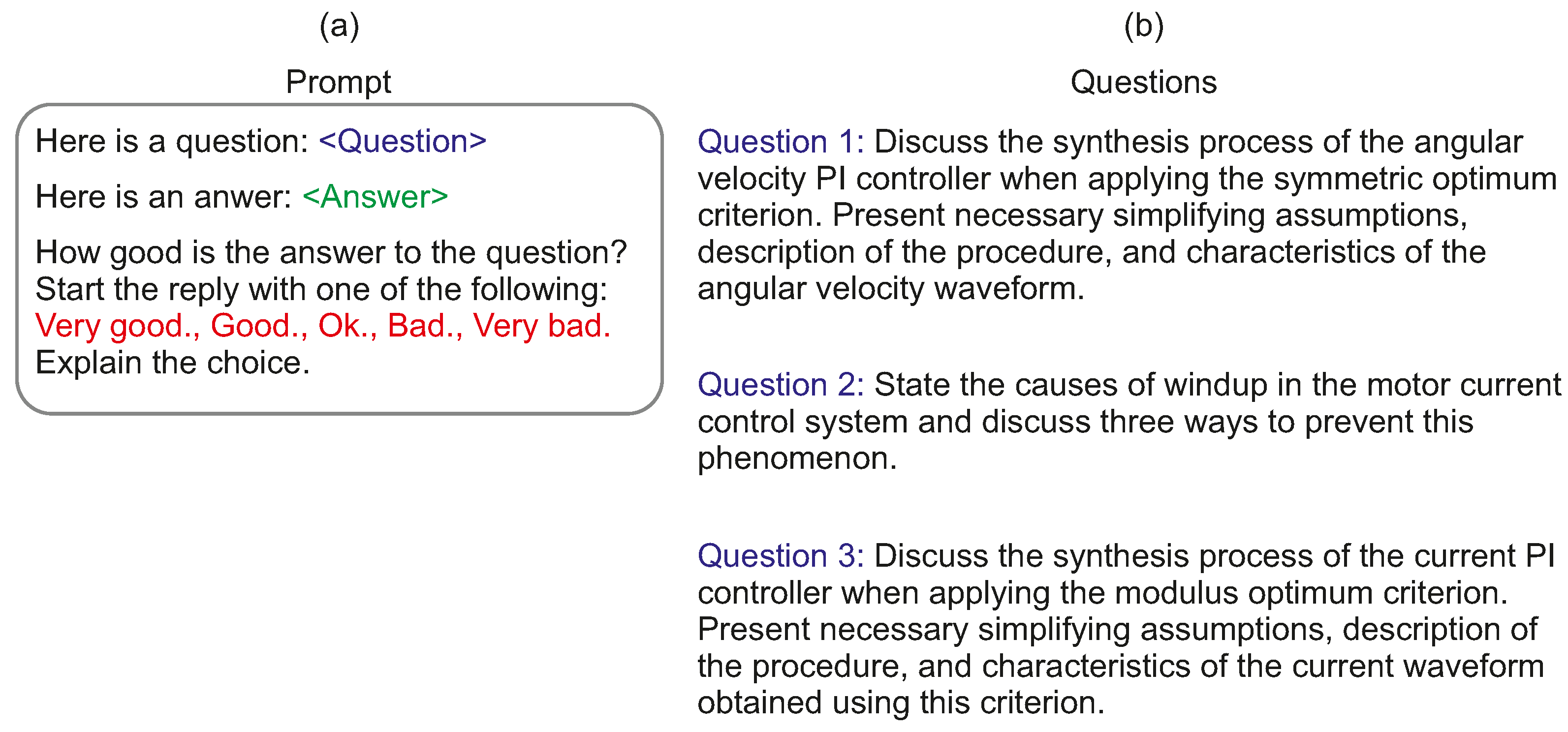
2.3.3. LLM-Based Tuning

By reasoning, learning, and incorporating knowledge into pre-trained neural networks, large language models are changing human–machine interactions and improving work in many areas [40]. The natural language generation and question-answering abilities are also very desirable advantages in search engines and intelligent customer services [30]. The above-mentioned properties make it advisable to verify the usefulness of LLMs in the controller’s tuning task.

With this approach, it was decided that the Tuning Assistant (TA) based on LLMs would be developed and investigated. As a base of the proposed TA, the AI Assistant from Ordemio has been chosen due to the learning ability from multiple data sources, simple development process, no hallucinations, and no-cost operations (with restrictions) [41].

In the first stage, based on the authors’ experience, a dataset was selected, and respective articles were loaded to the TA knowledge. Since the considered task is related to the tuning process of the angular velocity and current controllers for the PMSM drive, it was decided to load the paper where the magnitude optimum and the symmetric optimum criterion are described [25]. The work with the IMC approach was also included since this method can be successfully applied to current control [26]. To provide information about the PID controller’s structures, ref. [37] was introduced as an additional source. In this case, the URL pointed directly to the open-access version of the article. Finally, the dataset was augmented by two papers using the above-mentioned control methods in the PMSM drive [35,42]. The results obtained for the assistant trained using such a dataset are discussed later in the paper.

In the second stage, the TA was re-trained to examine if the reasoning and answering abilities could be improved. Here, additional pre-processed information related to the tuning procedure and presented in Section 2.1, Section 2.2 and in Section 2.3.1 was used.

The Tuning Assistant trained in this way is used to support the selection of CCS coefficients, and the results are shown in the following section along with state-of-the-art LLMs, namely OpenAI ChatGPT and Microsoft Copilot. The developed Tuning Assistant is available at http://fizyka.umk.pl/~ttarczewski/ta.html (accessed on 5 January 2025). The developed Tuning Assistant is shown in Figure 5. For the user’s convenience, suggested questions appear in the window, but it is also possible to enter your own prompt.

3. Results

Tuning methods for the cascade control structure equipped with PI-type current and angular velocity controllers for the PMSM drive described in the previous section have been investigated. A group of electrical engineers with different experience levels were invited to tune a model of the PMSM drive. Their experience has been divided into two levels: beginners and advanced users. The group of beginners consists of third-year bachelor students from automatics and robotics. Overall, they have a fundamental knowledge of the control of electrical drives and limited practical experience in this field. The second group included fifth-year master’s students, people with master’s degrees, and Ph.D. holders with several years of experience. The main parameters of the PMSM drive used in the considered task are listed in

Table A1. Parameters of the PMSM drive.

Symbol	Value	Unit		Symbol	Value	Unit
$I_N$	4	A		p	3	-
$T_{eN}$	4.6	Nm		$B_m$	0.014	Nms/rad
$R_s$	1.05	$\Omega$		$J_m$	0.0177	${\mathrm{kgm}}^2$
$L_s$	0.0127	H		$K_p$	100	-
${\Psi }_f$	0.25	Wb		$f_s$	22,000	Hz
$K_t$	1.145	Nm/A		$T_s$	4.55	μs

. As the reference signal, the angular velocity step from 0 rad/s to 3 rad/s at 50 ms has been applied. To investigate the disturbance compensation ability, the load torque step variations were introduced. Its value is equal to 3 Nm in the time period 200 ÷ 400 ms and 0 Nm outside this period. The above-mentioned values were set as initial ones. However, it was found that the electrical engineers did not modify these during the tuning task. The model of the PMSM drive developed in the Matlab/Simulink environment was shared with the user invited to accomplish the tuning task.

Received sets of controller parameters, along with additional explanations, including the drive performance (i.e., $ITS{E}_{\omega }$ performance index), number of attempts, and time required to accomplish the considered task, were analyzed, and these are listed in

Table 1. Parameters of the angular velocity and the currents PI controllers obtained by the users.

No.	${\mathit{k}}_{\mathbf{pi}}$	${\mathit{k}}_{\mathit{i}\mathit{i}}$	${\mathit{k}}_{\mathbf{ai}}$	${\mathit{k}}_{\mathit{p}\mathit{\omega }}$	${\mathit{k}}_{\mathit{i}\mathit{\omega }}$	${\mathit{k}}_{\mathit{a}\mathit{\omega }}$	${\mathbf{ITSE}}_{\mathit{\omega }}$	Auto-Tuning *	Method	Iter. no.	Time [mins]	User exp.	Figure
1	5.58	82.85	1	30.89	1000	1	0.00197	N	TA	–	≈1	adv	Figure 9e,f
2	0.5	200	1	30	200	1	0.00198	Y	empirical	74	80	beg	–
3	0.9	45	0	350	4	0.8	0.00198	Y	empirical	80	–	beg	–
4	217.15	0	371.45	134.49	500	3.16	0.00198	Y	ABC	500	70	adv	Figure 6e,f
5	0.39	144.44	0.1	210.1	0.0001	1	0.00199	N	analytical	80	–	beg	–
6	8.37	0.0001	1000	382.29	0.0004	100	0.002	N	analytical	109	30	beg	Figure 7e,f
7	2.79	82.85	0.8	152.72	1098	0.5	0.002	N	analytical	32	–	beg	–
8	278.96	82.85	3.37	388.98	388.98	1	0.0021	N	ChatGPT	–	≈3	adv	Figure 9a,b
9	0.56	82.72	0.8	15.29	109.86	1.12	0.0021	N	analytical	41	50	beg	–
10	0.5	231.11	7	15.29	109.86	1.27	0.0021	N	analytical	70	–	beg	–
11	0.23	82.72	0	152.97	0.0009	20	0.0021	N	analytical	34	71	beg	–
12	0.28	120.7	1	16.97	549.31	50	0.0022	N	analytical	27	–	beg	–
13	2.8	82.7	0	5493.1	0.0002	5	0.0022	N	analytical	37	56	beg	–
14	2.5	12.5	0.7	17.5	25	1.25	0.0023	N	empirical	42	15	adv	–
15	0.5	60	62	10	120	190	0.0026	Y	empirical	120	–	beg	–
16	1	300	5	20	100	40	0.0026	Y	empirical	93	–	adv	–
17	0.4	185	30	150	90	30	0.003	N	empirical	115	75	beg	–
18	0.75	38.52	0	44.7	92.52	0	0.003	N	analytical	98	–	beg	–
19	0.47	963.65	19.56	5.81	94.45	19.96	0.003	N	analytical	14	–	adv	Figure 7c,d
20	0.056	82.85	0.7	17.5	27.5	1.5	0.0032	N	an. & em.	55	10	adv	–
21	0.35	750	200	100	110	190	0.0034	Y	empirical	91	60	beg	–
22	1.21	44.95	1	7.73	45.14	15	0.0042	Y	PSO	2757	120	adv	Figure 6c,d
23	0.103	82.72	0	5	50	1	0.0044	N	an. & em.	–	45	adv	Figure 7a,b
24	1.4	82.72	0	15.29	1.4	5	0.0045	Y	analytical	47	66	beg	–
25	0.36	250	65	75	30	100	0.0091	Y	empirical	238	75	beg	–
26	0.019	11.88	40.42	9.47	37.86	189.86	0.013	N	ABC *	430	24	adv	Figure 6a,b
27	0.011	82.72	0.1	3.05	0.046	0	0.054	N	analytical	13	48	beg	–
28	0.28	82.85	1	0.3	0.8	1	3.22	N	an. & em.	21	16	adv	–
29	0.64	3.81	3.81	0.16	0.12	0.12	10.72	N	Copilot	–	≈2	adv	Figure 9c,d

* The coefficients obtained from ABC (row 26) were applied if auto-tuning was used.

. The following colors were used to indicate selected data: red for swarm-based tuning, green for analytical-based tuning, and blue for LLM-based tuning. These results are presented as waveforms and are described in the later part of this section.

From the obtained results, it can be seen that the empirical approach is most often used together with auto-tuning. The mean value of the iteration number is equal to 116, and the mean time needed to accomplish the task is equal to 73 min. Significantly fewer iterations are observed if the empirical approach; the mean value of the iteration number equals 45. In such a case, the time required to tune the control structure is also shorter; the task lasts ca. 58 min. The highest number of iterations is obtained for SBMA’s, but this approach does not directly involve the users. Here, the task is accomplished in ca. 62 min, and the users reported that most of this time was spent on the integration of the drive’s model with the optimization procedure and developing the proper performance index to be optimized. Therefore, it is expected that another tuning attempt would take less time, as in the case of the solution from row 26 used as the initial set from auto-tuning by the users. The fastest responses related to the considered tuning task were received from LLMs. Copilot needs ca. 2 min, ChatGPT gives the responses after ca. 3 min, while the answer from TA powered by Ordemio came after ca. 1 min. The conversation concerned tuning the current regulator, tuning the angular velocity controller, reducing possible overshoot, and selecting the anti-windup coefficient. The recording form conversations with LLMs are available to the reader as Supplementary Material attached to the paper.

It has been noted that there is a relationship between the chosen approach and the user experience. Beginners most often used the empirical approach supported by auto-tuning. Advanced users rather prefer analytical methods, but the Ziegler–Nichols method-based approach with manual fine-tuning can also be found in the considered group. Swarm-based tuning came from advanced users only. Finally, it was found that beginner users mainly focus on minimizing the $ITS{E}_{\omega }$ index, which leads to relatively large controller coefficients, which can lead to current oscillations in the transient and noisy operation of the drive. In the case of advanced users, a compromise between performance index minimization and secondary requirements related to signal oscillations is observed, resulting in relatively lower controller coefficients. Selected results from Table 1 are presented as waveforms and described in the following subsections.

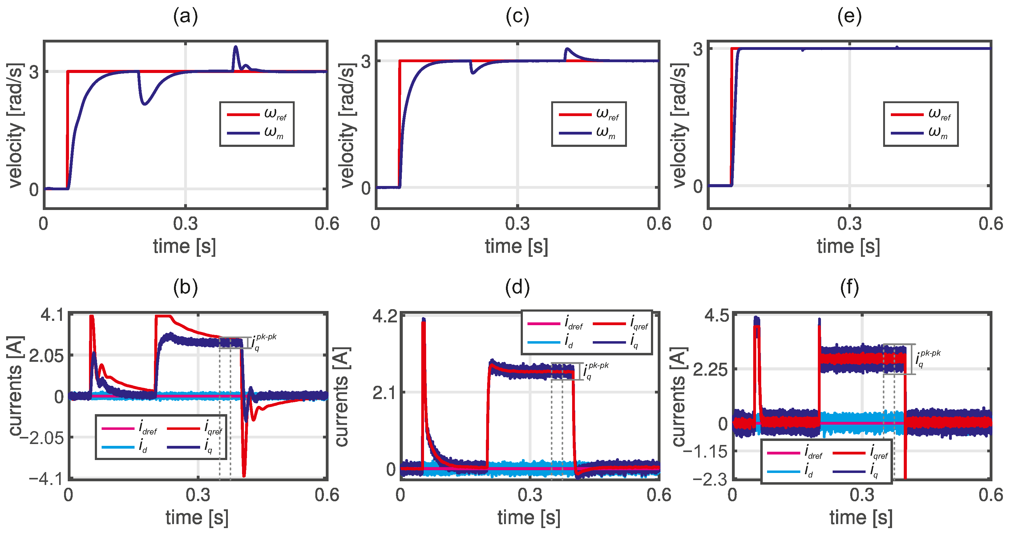
3.1. Swarm-Based Tuning

From Figure 6, it can be seen that a slightly different behavior has been obtained. All coefficients were simultaneously tuned along with anti-windup gains in this approach, but different performance indexes have been applied during optimization.

Figure 6. Step responses of PMSM drive with cascade control structure tuned using swarm-based optimization algorithms: (a,b)—ABC * (row 26 in Table 1), (c,d)—PSO (row 22 in Table 1), (e,f)—ABC (row 4 in Table 1). The first row is the angular velocity, and the last row is the space vector current components.

Figure 6. Step responses of PMSM drive with cascade control structure tuned using swarm-based optimization algorithms: (a,b)—ABC * (row 26 in Table 1), (c,d)—PSO (row 22 in Table 1), (e,f)—ABC (row 4 in Table 1). The first row is the angular velocity, and the last row is the space vector current components.

It is worth noting that results from the left column are obtained for the ABC optimization algorithm, and these were used as the initial set for users if needed. In this case, both the angular velocity step response and the load torque compensation are average, so there is space for performance improvement. On the other hand, the current ripples are relatively small. The optimization procedure lasted 24 min, and 430 iterations were completed in this amount of time. The performance index used in this approach is described by (15). The control parameters of the ABC are listed in

Table A2. Parameters of the ABC.

Parameter	Symbol	Value
No of optimized parameters	D	6
No of colony size	NP	10
No of food sources	FN	NP/2
Maximum no of cycles	MCN	20
Control parameter limit	limit	FN × D
Scout production period	SPP	FN × D
Modification rate	MR	0.8

. It is worth noting that the parameters were selected in accordance with the information provided in [43].

Results shown in the center column (see Figure 6c,d) are obtained for the PSO optimization algorithm. According to the user’s response with advanced experience, the tuning process took ca. 120 min, but most of the time was spent adapting PSO to the considered control system. It is worth noting that all coefficients of the control structure were simultaneously tuned along with anti-windup gains. One can see a much better control performance compared to the results obtained for the ABC control scheme. Moreover, the current ripple seems to be acceptable, and a compromise between dynamic behavior and the noise of the drive has been achieved after 2757 iterations. The performance index used in this case was similar to (15), but the second component responsible for elimination d-axis steady-state error has been omitted, and the absolute value of the angular velocity error has been used instead of square one.

In the case of the results shown in the right column, the ABC control algorithm has also been used. In this case, the overall time needed to accomplish this task was ca. 70 min, but the advanced user responded that the tuning time lasted ca. 5 min. It is also caused by using initial gain coefficients. From the angular speed response, it can be seen that the rise time and the load torque compensation are superior. On the other hand, the current ripple observed in Figure 6f seems to be unacceptable. The reason is a simple performance index used in an optimization scheme, where the Integral of Absolute Error (IAE) from the difference between actual and reference velocity has been minimized. The lack of the component responsible for chattering attenuation is visible in the drive response. The obtained controller’s coefficients and calculated $ITS{E}_{\omega }$ performance index are listed in Table 1 and marked in red.

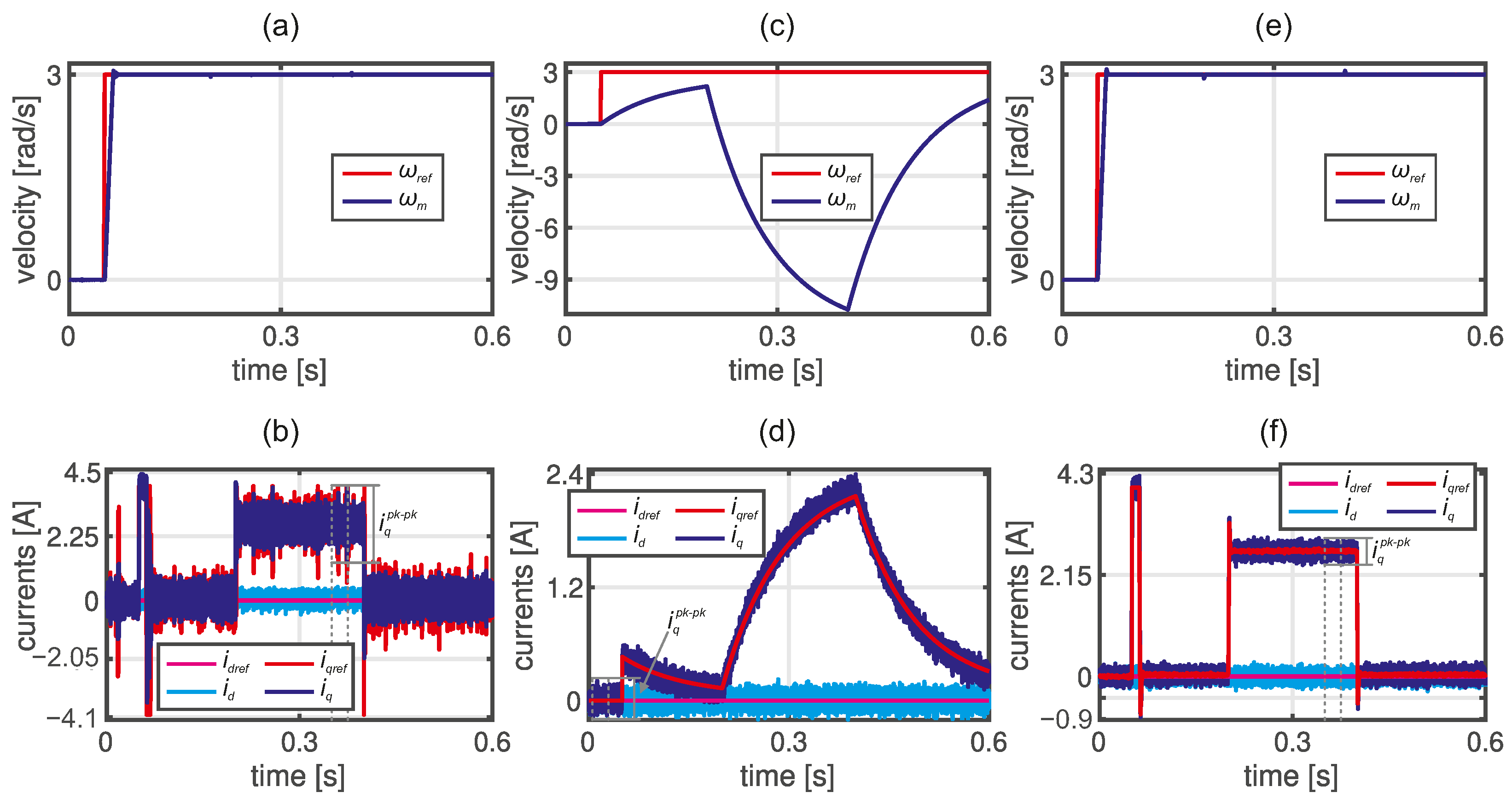
3.2. Analytical-Based Tuning

The first example of the tuning results obtained for the analytical approach is shown in the left column in Figure 7. In this case, the IMC was used for the current control loop, while the symmetric optimum criteria were utilized for the outer loop. Finally, the obtained coefficients were fine-tuned according to the Ziegler–Nichols approach. In this case, the beginner user did not use the initial coefficients obtained from auto-tuning supported by ABC. The dynamic performance of the angular velocity response and load torque compensation is acceptable. The main disadvantage of the proposed set of coefficients is the windup phenomenon. The level of current ripples is acceptable. The tuning procedure lasted 45 min, and a simplified drive model was utilized during the fine-tuning.

Figure 7. Step responses of PMSM drive with cascade control structure tuned using analytical criteria: (a,b)—analytical and empirical (row 23 in Table 1), (c,d)—analytical (row 19 in Table 1), (e,f)—analytical (row 6 in Table 1). The first row is the angular velocity, and the last row is the space vector current components.

Figure 7. Step responses of PMSM drive with cascade control structure tuned using analytical criteria: (a,b)—analytical and empirical (row 23 in Table 1), (c,d)—analytical (row 19 in Table 1), (e,f)—analytical (row 6 in Table 1). The first row is the angular velocity, and the last row is the space vector current components.

Results shown in the center column in Figure 7c,d are obtained for the root locus method. The superior load torque compensation and drive dynamics have been obtained along with the low level of current ripples. Moreover, the advanced user needs only 14 iterations to obtain the final coefficients of controllers.

In the case of the results shown in the right column in Figure 7, these are obtained by the beginner user in the analytical approach (i.e., IMC and symmetric optimum criteria). The number of iterations equals 109, and the overall tuning process, including manual fine-tuning of the current controllers, lasts ca. 30 min. The dynamic performance of the angular velocity control is superior but not applicable in the real drive. Unacceptable current ripples are also observed. Quite similar results are obtained for half of the responses received from beginner users in the tuning task. They are focused on the superior angular velocity response, and secondary requirements are not considered. The obtained controller’s coefficients and calculated $ITS{E}_{\omega }$ performance index are listed in Table 1 and marked in green.

3.3. LLM-Based Tuning

As stated before, the efficiency of the developed TA was compared with the state-of-the-art LLMs, namely ChatGPT from OpenAI and Copilot from Microsoft. To obtain objective results from the LLMs, the same questions have been asked in the manner shown in Figure 8.

Figure 8. LLM evaluation flowchart.

Figure 8. LLM evaluation flowchart.

From Figure 8, it can be seen that the questions were asked in a manner typical of cascade control structure tuning, i.e., from the inner to the outer control loop. In the case of an incorrect or incomplete answer, an auxiliary question was asked. It was marked with a rectangle with a dashed line. If the answers were too generic, the question was edited and asked again. The final results obtained from the conversations with the state-of-the-art LLMs and the proposed Tuning Assistant are shown below. The recording of the conversations is accessible to the reader as Supplementary Material attached to the paper, while the prompts used in the tuning task are listed in

Table A3. Prompts used in the tuning task.

ChatGPT	Copilot	Tuning Assistant
1. How should I tune the current PI controller for the PMSM drive?	1. How should I tune the current PI controller for the PMSM drive?	1. How should I tune the current PI controller for the PMSM drive?
2. OK, I observe an overshoot during velocity transient and current ripple during steady-state. What do you suggest?	2. Ok, can you calculate the proportional gain and the integration time constant of the PI current controller if I give you a rise time and basic parameters of the motor?	2. Ok, I prefer the current control without overshoot, could you please give me the formulas for PI current controller?
3. I noticed that I have zero anti-windup coefficients in both control loops. How do I choose them?	3. Ok, R = 1.05, L = 0.0127, and Tr = 0.005	3. Thanks. I need clarification on the current rise in time value.
	4. Ok, how to determine the optimal value of the Proportional Gain (Kp) of the velocity controller in PMSM for the moment of inertia equal to 0.0177 [kgm·m] and torque constant equal to 1.1447 [Nm/A]	4. Thanks, how should I tune the velocity PI controller for the PMSM drive?
	5. Thanks. And what about the optimal value of the Integral Gain (ki) for this velocity controller?	5. I noticed that I have zero anti-windup coefficients in both control loops. How do I choose them?
	6. I noticed that I have zero anti-windup coefficients in both control loops. How do I choose them?

.

Results obtained for controller’s coefficients from the OpenAI ChatGPT conversation are shown in the left column in Figure 9 (date of access: 25 September 2024). Unacceptable current ripples are observed, and the angular velocity has high dynamics in this case. These are caused by relatively huge proportional coefficients of both controllers. In the first version of the response, the anti-windup coefficients have not been pointed out. After additional conversation, formulas for the anti-windup coefficients were depicted, resulting in drive behavior presented in Figure 9a,b. The conversation with ChatGPT is presented in the recording.

Figure 9. Step responses of PMSM drive with cascade control structure tuned using LLMs: (a,b)—ChatGPT (row 8 in Table 1), (c,d)—Copilot (row 29 in Table 1), (e,f)—Tuning Assistant (row 1 in Table 1). The first row is the angular velocity, and the last row is the space vector current components.

Figure 9. Step responses of PMSM drive with cascade control structure tuned using LLMs: (a,b)—ChatGPT (row 8 in Table 1), (c,d)—Copilot (row 29 in Table 1), (e,f)—Tuning Assistant (row 1 in Table 1). The first row is the angular velocity, and the last row is the space vector current components.

Results shown in the center column (see Figure 9c,d) are obtained from Microsoft Copilot available in Microsoft Edge (date of access: 2 October 2024). Poor dynamics of the angular velocity control and poor load torque compensation are observed for the obtained set of coefficients. Such behavior is caused by a relatively small value of the controller’s coefficients. As in the case of the ChatGPT response, the anti-windup coefficients have not been pointed out. After additional conversation, formulas for the anti-windup coefficients were depicted, resulting in drive behavior presented in Figure 9c,d. The conversation with Microsoft Copilot is presented in the recording, from the time of 3:16 s.

Finally, the results shown in the right column in Figure 9 are obtained from the Tuning Assistant powered by Ordemio. In this case, both the angular velocity dynamics and load torque compensation are superior. The current ripples are acceptable. The learning ability of this assistant has been proven in this case. The conversations with the TA are also presented in the recording. They are shown from the time of 5:44 s in the first conversation, and the time of 7:03 s in the final conversation with the re-trained TA powered by Ordemio. The controller’s coefficients obtained for LLM-based tuning and calculated $ITS{E}_{\omega }$ performance index are listed in Table 1 and marked in blue.

3.4. Quantitative Analysis

3.4.1. Prompt Scoring

As shown in [44,45], the prompt scoring approach can be applied to the quantitative analysis of LLMs, including some aspects of robustness, i.e., misclassification [46]. This method belongs to Zero-shot Assessment, and it is based on asking LLMs to assign an absolute score to each considered text. Such an approach requires creating prompts in which LLMs are asked to assess the response quality on the imposed scale [44]. Next, the ratings are compared with the human scores [45], and the gap between the human and LLM scores is calculated. To assess the developed Tuning Assistant and other LLMs used in this paper, a simple prompt is used with the general template shown in Figure 10a. The answers for questions depicted in Figure 10b came from the students’ exams. Previously graded examinations on the subject of Automatic Control of Electrical Drives were selected, and the answers were used for quantitative assessment due to the content being similar to the considered tuning task.

First, it was investigated how much the LLMs and Tuning Assistant deviated from the human, i.e., educator, across all graded answers. To accomplish this, the scores from LLMs (i.e., Very bad, Bad, Ok, Good, Very Good) and from the educator were scaled to be between 0 and 1. Next, a gap between the human’s and LLM’s scores is calculated, and this is presented in Figure 11.

From the obtained results, it can be seen that there are no significant differences between scores obtained from the educator from LLMs and the Tuning Assistant. It was found that 33% of the grades given by ChatGPT are the same as the human ratings. Copilot gave 40% the same rating as the human, while the agreement between the Tuning Assistant and the human’s ratings was 47%. A discrepancy of one rating was obtained for 60% of results for Copilot and for 47% of results for the TA and ChatGPT. The largest discrepancy observed was two ratings and was obtained for 20% of the results for ChatGPT and only for 6% of the responses for the proposed Tuning Assistant. It was also found that the highest discrepancies occurred for extreme ratings. From the above-mentioned quantitative analysis based on the prompt scoring approach, it can be concluded that a satisfactory correlation between human and LLM-based approaches is observed, while the best accuracy is obtained for the developed Tuning Assistant.

3.4.2. Torque Ripple

To provide analysis of the obtained results in terms of the torque ripple generation, it was decided to investigate the torque ripple factor ($TRF$) [16,47], defined as the ratio of the peak-to-peak torque ripple in a steady-state to the rated torque:

$$TRF={\displaystyle \frac{T_e^{pk-pk}}{T_{eN}}}\times 100\%$$

(16)

with $T_e^{pk-pk}=K_t{i}_q^{pk-pk}$, where $i_q^{pk-pk}$ is the peak-to-peak torque ripple in a steady-state, as marked in Figure 6, Figure 7, and Figure 9, respectively. The rated torque $T_{eN}$ for the considered motor is listed in Table A1, while the q-axis current’s, the torque’s ripples, and the calculated $TRF$ are listed in

Table 2. Torque ripple factor calculated for steady-state drive operation.

No.	Figure	Method	${\mathit{i}}_{\mathit{q}}^{\mathit{pk}-\mathit{pk}}$ [A]	${\mathit{T}}_{\mathit{e}}^{\mathit{pk}-\mathit{pk}}$ [Nm]	$\mathit{TRF}$ [%]
1	Figure 6b	ABC	0.46	0.53	11.5
2	Figure 6d	PSO	0.47	0.54	11.8
3	Figure 6e	ABC	1.12	1.28	27.9
4	Figure 7b	analytical and empirical	0.54	0.62	13.5
5	Figure 7d	analytical	0.46	0.53	11.6
6	Figure 7e	analytical	1.25	1.43	31.2
7	Figure 9b	ChatGPT	2.71	3.10	67.7
8	Figure 9d	Copilot	0.44	0.50	10.9
9	Figure 9e	Tuning Assistant	0.57	0.65	14.2

.

From the obtained results, it can be seen that the lowest $TRF$ values are at the level of 10.9 (Copilot) to 14.2 (Tuning Assistant). It is expected that higher $TRF$ values will produce noise and vibrations of the drive [15,16], and therefore, these are not recommended for implementation. Finally, it should be pointed out that a trade-off between current/torque ripples, load torque compensation, and dynamic behavior of the drive is required. For that reason, results obtained for Copilot are also not recommended for implementation due to poor dynamics of the angular velocity control and poor load torque compensation.

4. Discussion

The paper described a novel Tuning Assistant based on the large language model. A two-stage training process was described, along with dataset preparation. The ability to reason and answer questions in the PMSM drive tuning task has been confirmed.

The reason for developing and examining the TA is that the state-of-the-art LLMs do not provide correct answers, resulting in poor dynamics properties and/or unacceptable torque ripples, as shown in Figure 9. The tested LLMs give answers of a general nature, can be misleading, and do not provide valuable solutions for the analyzed problem. It is possible to improve the performance of the state-of-the-art LLMs by using the fine-tuning approach. According to [48], performance improvement depends on several factors such as topic alignment, prompt formulation, sample sizes, and the quality of fine-tuning samples, and it requires access to the LLM structure [49]. The proposed Tuning Assistant outperforms other LLMs, is available online, and can be used by the users if needed. The results also indicate that by using the pre-processed dataset containing a synthetic description from the highest-quality research papers, the reasoning and answering abilities of the Tuning Assistant can be improved. The accuracy of the developed Tuning Assistant has also been confirmed by quantitative analysis based on the prompt scoring approach. These can also be used to investigate the robustness in terms of misclassification [46].

As shown in Figure 6, SBMA can successfully support the tuning procedure. However, the final result is strongly related to the performance index used. If the developed function takes into account secondary requirements related to the drive behavior, better results are achieved. This solution is recommended for more advanced users who can integrate knowledge from the area of electric drive control and optimization.

It is expected that the proposed Tuning Assistant will be used by users with limited experience. Since the correct analysis of the obtained waveform and knowledge of the capabilities and limitations of the control object is required to formulate appropriate prompts and improve the drive’s performance, it was decided to prepare some suggested questions to help users when creating a prompt.

5. Conclusions

Received from electrical engineers, sets of CCS parameters indicate that users with relatively low experience do not take into account secondary requirements, resulting in non-proper drive operation. They often focus on superior dynamics of the angular velocity, which can lead to current oscillations in the transient and noisy operation of the drive. If the empirical approach is employed, the number of attempts is high, and the time needed to accomplish the tuning task is relatively long. This group of users does not prefer the swarm-based tuning due to the lack of knowledge in the field of optimization methods and lack of experience in a selection of SMBA’s control parameters such as colony size, particle partitioning within the colony, ranges of optimized parameters, and the ability to impose constraints on selected signals in the drive during optimization. In the author’s opinion, the developed Tuning Assistant can fill the gap and support the tuning procedure in the case of less experienced users.

Electrical engineers with greater experience obtain better results in a shorter time. Even if the quality indicator does not reach the minimum value, the drive behavior is very good, and the secondary requirements are usually taken into account. The results obtained from this user group are related to applying analytical methods and giving good initial results after relatively simple calculations.

The Tuning Assistant has been developed to make it easier for less experienced users to use analytical methods. The obtained results indicate that by using the pre-processed dataset, the reasoning and answering abilities of TA can be improved, giving proper and accurate solutions in a tuning task. The proposed approach can also be used in applications where analytical tuning methods exist. In such a case, the respective dataset should be created, and the Tuning Assistant should be retrained.

One of the future directions of work in this field could be the semi-automatic preparation of the datasets. In this concept, humans will select representative scientific papers, manuals, and datasheets in the first step. Next, the LLM will be asked to prepare a summary containing the most important aspects of the problem under consideration (controller tuning, in this case). Finally, after being accepted by the human, the training dataset prepared in this way will be used in the assistant’s training process. Once relatively large datasets are developed, these can be used to assess the robustness and fine-tuning of LLMs and TA. Future research directions will also be focused on developing, implementing, and validating training sets with tuning methods for complex controllers (e.g., state feedback, model predictive) used in electrical drives. It is also planned to use AI-supported image recognition in the controller tuning process for visual evaluation and shaping the drive’s responses in the time and frequency domains.

References

1. Huanhuan, R.; Zhang, L.; Su, C.; Jian, S.; Liu, D. Research on fuzzy control of permanent magnet synchronous motor for a mobile robot. In Proceedings of the Journal of Physics: Conference Series; IOP Publishing: Bristol, UK, 2021; Volume 1754, p. 012172. [Google Scholar]
2. Li, P.; Xu, X.; Yang, S.; Jiang, X. Open circuit fault diagnosis strategy of PMSM drive system based on grey prediction theory for industrial robot. Energy Rep. 2023, 9, 313–320. [Google Scholar] [CrossRef]
3. Che, X.; Ma, Z.; Qi, X.; Li, W.; Niu, H.; Yan, C. Barrier-Function-Based Adaptive Fast-Terminal Sliding-Mode Control for a PMSM Speed-Regulation System. Electronics 2024, 13, 1091. [Google Scholar] [CrossRef]
4. Farah, N.; Lei, G.; Zhu, J.; Guo, Y. Robust Model-Free Reinforcement Learning Based Current Control of PMSM Drives. IEEE Trans. Transp. Electrif. 2024, 1. [Google Scholar] [CrossRef]
5. Di Fonso, R.; Cecati, C. Navigation and Motors Control of a Differential Drive Mobile Robot. In Proceedings of the 2023 International Conference on Control, Automation and Diagnosis (ICCAD), Rome, Italy, 10–12 May 2023; pp. 1–6. [Google Scholar] [CrossRef]
6. Wang, Y.; Fang, S.; Hu, J. Active disturbance rejection control based on deep reinforcement learning of PMSM for more electric aircraft. IEEE Trans. Power Electron. 2022, 38, 406–416. [Google Scholar] [CrossRef]
7. Aggarwal, A.; Meier, M.; Strangas, E.; Agapiou, J. Analysis of Modular Stator PMSM Manufactured Using Oriented Steel. Energies 2021, 14, 6583. [Google Scholar] [CrossRef]
8. Tarczewski, T.; Szczepanski, R.; Erwinski, K.; Hu, X.; Grzesiak, L.M. A Novel Sensitivity Analysis to Moment of Inertia and Load Variations for PMSM Drives. IEEE Trans. Power Electron. 2022, 37, 13299–13309. [Google Scholar] [CrossRef]
9. Ewert, P.; Kowalski, C.T.; Jaworski, M. Comparison of the Effectiveness of Selected Vibration Signal Analysis Methods in the Rotor Unbalance Detection of PMSM Drive System. Electronics 2022, 11, 1748. [Google Scholar] [CrossRef]
10. Zuo, Y.; Lai, C.; Iyer, K.L.V. A review of sliding mode observer based sensorless control methods for PMSM drive. IEEE Trans. Power Electron. 2023, 38, 11352–11367. [Google Scholar] [CrossRef]
11. Wróbel, K.; Szabat, K.; Wicher, B.; Brock, S. Hybrydowy ślizgowy obserwator Luenbergera w układzie napędowym z połączeniem elastycznym. Przeglad Elektrotechniczny 2024, 2024, 104–107. [Google Scholar] [CrossRef]
12. Kaminski, M.; Malarczyk, M. Hardware implementation of neural shaft torque estimator using low-cost microcontroller board. In Proceedings of the 2021 25th International Conference on Methods and Models in Automation and Robotics (MMAR), Międzyzdroje, Poland, 23–26 August 2021; IEEE: Warszawa, Poland, 2021; pp. 372–377. [Google Scholar]
13. Jankowska, K.; Dybkowski, M. Experimental Analysis of the Current Sensor Fault Detection Mechanism Based on Neural Networks in the PMSM Drive System. Electronics 2023, 12, 1170. [Google Scholar] [CrossRef]
14. Jin, L.; Mao, Y.; Wang, X.; Lu, L.; Wang, Z. Online Data-Driven Fault Diagnosis of Dual Three-Phase PMSM Drives Considering Limited Labeled Samples. IEEE Trans. Ind. Electron. 2023, 71, 6797–6808. [Google Scholar] [CrossRef]
15. Niewiara, L.J.; Szczepanski, R.; Tarczewski, T.; Grzesiak, L.M. State Feedback Speed Control with Periodic Disturbances Attenuation for PMSM Drive. Energies 2022, 15, 587. [Google Scholar] [CrossRef]
16. Qian, W.; Panda, S.K.; Xu, J.X. Torque ripple minimization in PM synchronous motors using iterative learning control. IEEE Trans. Power Electron. 2004, 19, 272–279. [Google Scholar] [CrossRef]
17. Chung, D.W.; Sul, S.K. Analysis and compensation of current measurement error in vector-controlled AC motor drives. IEEE Trans. Ind. Appl. 1998, 34, 340–345. [Google Scholar] [CrossRef]
18. Tarczewski, T.; Niewiara, L.; Grzesiak, L. Artificial bee colony based state feedback position controller for PMSM servo-drive—The efficiency analysis. Bull. Pol. Acad. Sci. Tech. Sci. 2020, 68, 997–1007. [Google Scholar] [CrossRef]
19. Templos-Santos, J.L.; Aguilar-Mejia, O.; Peralta-Sanchez, E.; Sosa-Cortez, R. Parameter Tuning of PI Control for Speed Regulation of a PMSM Using Bio-Inspired Algorithms. Algorithms 2019, 12, 54. [Google Scholar] [CrossRef]
20. Aguilar-Mejía, O.; Minor-Popocatl, H.; Tapia-Olvera, R. Comparison and ranking of metaheuristic techniques for optimization of PI controllers in a machine drive system. Appl. Sci. 2020, 10, 6592. [Google Scholar] [CrossRef]
21. Hussain, H.A. Tuning and Performance Evaluation of 2DOF PI Current Controllers for PMSM Drives. IEEE Trans. Transp. Electrif. 2021, 7, 1401–1414. [Google Scholar] [CrossRef]
22. Ren, J.; Ye, Y.; Xu, G.; Zhao, Q.; Zhu, M. Uncertainty-and-Disturbance-Estimator-Based Current Control Scheme for PMSM Drives with a Simple Parameter Tuning Algorithm. IEEE Trans. Power Electron. 2017, 32, 5712–5722. [Google Scholar] [CrossRef]
23. Rajesh Kumar Mahto, A.M.; Bansal, R.C. Controller design using PSO and WOA algorithm for enhanced performance of vector-controlled PMSM drive. Int. J. Model. Simul. 2024. [Google Scholar] [CrossRef]
24. Achour, H.B.; Ziani, S.; Chaou, Y.; El Hassouani, Y.; Daoudia, A. Permanent magnet synchronous motor PMSM control by combining vector and PI controller. WSEAS Trans. Syst. Control 2022, 17, 244–249. [Google Scholar] [CrossRef]
25. Umland, J.W.; Safiuddin, M. Magnitude and symmetric optimum criterion for the design of linear control systems: What is it and how does it compare with the others? IEEE Trans. Ind. Appl. 1990, 26, 489–497. [Google Scholar] [CrossRef]
26. Harnefors, L.; Nee, H.P. Model-based current control of AC machines using the internal model control method. IEEE Trans. Ind. Appl. 1998, 34, 133–141. [Google Scholar] [CrossRef]
27. Pietrusewicz, K.; Waszczuk, P.; Kubicki, M. MFC/IMC control algorithm for reduction of load torque disturbance in PMSM servo drive systems. Appl. Sci. 2018, 9, 86. [Google Scholar] [CrossRef]
28. Song, W.; Li, J.; Ma, C.; Xia, Y.; Yu, B. A Simple Tuning Method of PI regulators in FOC for PMSM Drives based on Deadbeat Predictive Conception. IEEE Trans. Transp. Electrif. 2024, 10, 9852–9863. [Google Scholar] [CrossRef]
29. Nasab, M.R.; Ghalebani, P.; Bruno, S.; Cometa, R.; La Scala, M. Adaptive PI Control of PMSM for Electric Vehicle Application Based on Sliding-mode Extremum Seeking Algorithm. In Proceedings of the 2023 Asia Meeting on Environment and Electrical Engineering (EEE-AM), Hanoi, Vietnam, 13 November 2023; IEEE: Ho Chi Minh City, Vietnam, 2023; pp. 1–6. [Google Scholar]
30. Chang, Y.; Wang, X.; Wang, J.; Wu, Y.; Yang, L.; Zhu, K.; Chen, H.; Yi, X.; Wang, C.; Wang, Y.; et al. A survey on evaluation of large language models. ACM Trans. Intell. Syst. Technol. 2024, 15, 1–45. [Google Scholar] [CrossRef]
31. Kevian, D.; Syed, U.; Guo, X.; Havens, A.; Dullerud, G.; Seiler, P.; Qin, L.; Hu, B. Capabilities of large language models in control engineering: A benchmark study on gpt-4, claude 3 opus, and gemini 1.0 ultra. arXiv 2024, arXiv:2404.03647. [Google Scholar]
32. de Zarzà, I.; de Curtò, J.; Roig, G.; Calafate, C.T. Llm adaptive pid control for b5g truck platooning systems. Sensors 2023, 23, 5899. [Google Scholar] [CrossRef]
33. Bobek, V. PMSM electrical parameters measurement. Free. Semicond. 2013, 7, 13. [Google Scholar]
34. Szczepanski, R.; Tarczewski, T.; Niewiara, L.J.; Stojic, D. Identification of mechanical parameters in servo-drive system. In Proceedings of the 2021 IEEE 19th International Power Electronics and Motion Control Conference (PEMC), Gliwice, Poland, 25–29 April 2021; IEEE: Warszawa, Poland, 2021; pp. 566–573. [Google Scholar]
35. Tarczewski, T.; Skiwski, M.; Grzesiak, L.M.; Zieliński, M. PMSM servo-drive fed by SiC MOSFETs based VSI. Power Electron. Drives 2018, 3, 35–45. [Google Scholar] [CrossRef]
36. Astrom, K.J.; Hagglund, T. PID controllers. In Theory, Design, and Tuning Problems; Instrument Society of America: Pittsburgh, PA, USA, 1995. [Google Scholar]
37. Bingi, K.; Ibrahim, R.; Karsiti, M.N.; Hassan, S.M.; Harindran, V.R. A comparative study of 2DOF PID and 2DOF fractional order PID controllers on a class of unstable systems. Arch. Control Sci. 2018, 28, 635–682. [Google Scholar] [CrossRef]
38. Dannehl, J.; Fuchs, F.W.; Thøgersen, P.B. PI state space current control of grid-connected PWM converters with LCL filters. IEEE Trans. Power Electron. 2010, 25, 2320–2330. [Google Scholar] [CrossRef]
39. Roni, M.H.K.; Rana, M.; Pota, H.; Hasan, M.M.; Hussain, M.S. Recent trends in bio-inspired meta-heuristic optimization techniques in control applications for electrical systems: A review. Int. J. Dyn. Control 2022, 10, 999–1011. [Google Scholar] [CrossRef]
40. Chen, J.; Liu, Z.; Huang, X.; Wu, C.; Liu, Q.; Jiang, G.; Pu, Y.; Lei, Y.; Chen, X.; Wang, X.; et al. When large language models meet personalization: Perspectives of challenges and opportunities. World Wide Web 2024, 27, 42. [Google Scholar] [CrossRef]
41. Web Page of a Software Solutions Provider That Enables Creating Custom GPT Chatbot. Available online: www.ordemio.com/ai-chatbot (accessed on 15 December 2024).
42. Tarczewski, T.; Grzesiak, L.M. Constrained State Feedback Speed Control of PMSM Based on Model Predictive Approach. IEEE Trans. Ind. Electron. 2016, 63, 3867–3875. [Google Scholar] [CrossRef]
43. Karaboga, D.; Basturk, B. Artificial bee colony (ABC) optimization algorithm for solving constrained optimization problems. In Proceedings of the International Fuzzy Systems Association World Congress, Cancun, Mexico, 18–21 June 2007; Springer: Berlin/Heidelberg, Germany, 2007; pp. 789–798. [Google Scholar]
44. Liusie, A.; Manakul, P.; Gales, M.J. Zero-shot NLG evaluation through pairware comparisons with llms. arXiv 2023, arXiv:2307.07889. [Google Scholar]
45. Schneider, J.; Schenk, B.; Niklaus, C. Towards llm-based autograding for short textual answers. arXiv 2023, arXiv:2309.11508. [Google Scholar]
46. Liu, Y.; Cong, T.; Zhao, Z.; Backes, M.; Shen, Y.; Zhang, Y. Robustness Over Time: Understanding Adversarial Examples’ Effectiveness on Longitudinal Versions of Large Language Models. arXiv 2023, arXiv:2308.07847. [Google Scholar]
47. Tarczewski, T.; Grzesiak, L. Torque ripple minimization for PMSM using voltage matching circuit and neural network based adaptive state feedback control. In Proceedings of the 2014 16th European Conference on Power Electronics and Applications, Lappeenranta, Finland, 26–28 August 2014; IEEE: Espoo, Finland, 2014; pp. 1–10. [Google Scholar]
48. Li, X.; Zhang, Y.; Malthouse, E.C. Exploring fine-tuning chatgpt for news recommendation. arXiv 2023, arXiv:2311.05850. [Google Scholar]
49. Latif, E.; Zhai, X. Fine-tuning ChatGPT for automatic scoring. Comput. Educ. Artif. Intell. 2024, 6, 100210. [Google Scholar] [CrossRef]
Figure 1. Drive’s current step responses.
Electronics 14 00232 g001
Figure 2. Drive’s velocity step response.
Electronics 14 00232 g002
Figure 3. Cascade control structure.
Electronics 14 00232 g003
Figure 4. SBMA’s general flowchart.
Electronics 14 00232 g004
Figure 5. Tuning Assistant’s window.
Electronics 14 00232 g005
Figure 10. Scoring template (a) and questions used for quantitative assessment (b).
Electronics 14 00232 g010
Figure 11. Gaps between human and LLM ratings in the prompt scoring task for (a), Question 1 (b), Question 2, and (c) Question 3.
Electronics 14 00232 g011