Abstract
This paper presents new fast discrete Krawtchouk transform (DKT) algorithms for input sequences of length 3 to 8. Small-sized DKT algorithms can be utilized in image processing applications to extract local image features formed by a sliding spatial window, and they can also serve as building blocks for developing larger-sized algorithms. Existing strategies to reduce the computational complexity of DKT mainly focus on modifying the recurrence relations for Krawtchouk polynomials, dividing the input signals into blocks or layers, or using different methods to approximate the coefficient values. Algorithms developed using the first two strategies are computationally intensive, which introduces a significant time delay in the computation process. Algorithms based on the approximation of polynomial coefficient values reduce computation time but at the expense of reduced accuracy. We use a different approach based on reducing the block structure of the matrix to one of the previously developed block-structural patterns, which allows us to factorize the resulting matrix in such a way that it leads to a reduction in the computational complexity of the synthesized algorithm. We describe the algorithmic solutions we have obtained through data flow graphs. The proposed DKT algorithms reduce the number of multiplications, additions, and shifts by an average of 58%, 27%, and 68%, respectively, compared to the direct computation of DKT via matrix-vector product. These characteristics were averaged across the considered input sizes (from 3 to 8).
1. Introduction
Currently, in signal and image processing, transforms based on orthogonal polynomials are being widely used [1]. In particular, the discrete Tchebichef transform is applied in image compression and video coding [2,3], as well as in text analysis [4]. Hahn moments are utilized for image classification [5,6], while Legendre moments are employed in image analysis and reconstruction [7,8]. Image moments obtained based on orthogonal polynomials are projections of an image function on a polynomial basis. They capture image object shape properties. That is why such moments are applied as local or global image features in image processing and computer vision [1,9]. One such feature set is the Krawtchouk moments, which is used in image watermarking [10,11,12,13], image analysis and reconstruction [6,14,15,16,17], face recognition [18], edge detection [19], data hiding [20], single-pixel imaging [21,22], and other applications. Krawtchouk moments can be extracted using the discrete Krawtchouk transform (DKT), which computes a weighted sum of signal samples or pixel intensities using Krawtchouk polynomials of various orders. Like other transforms based on orthogonal polynomials, the DKT shares properties of linearity and orthonormality and represents the signal in the spectral domain. Owing to the existence of the inverse DKT, the complete reconstruction of a signal is enabled.
In image processing, the use of the DKT often requires reducing computational complexity, especially in real-time or high-performance applications, such as three-dimensional (3D) object reconstruction [17] or face recognition [18]. This paper addresses the issue of saving arithmetic operations for one-dimensional DKT. Unlike trigonometric transforms, the elements of the DKT matrices depend not only on the discrete independent variable x and the degree n of Krawtchouk polynomials, which serve as the indices of these elements, but also on the localization parameter p. This parameter affects both the structure of the DKT matrices and the values of their elements. Therefore, the computational complexity of the DKT has often been reduced by applying algebraic transformations to the recursive formulas used to calculate Krawtchouk polynomial values for different p [23,24].
At the same time, the DKT algorithms for short-length input sequences can significantly decrease the time consumption of the local feature extraction in image processing and computer vision applications. Additionally, such algorithms can be exploited as building blocks for designing fast algorithms for large data sequences. For example, the Kronecker product of several smaller orthogonal matrices can be used to form a transform matrix for processing large data sequences when reducing the overall system complexity is crucial [25,26].
In this article, we consider a relevant problem of constructing fast DKT algorithms for short-length input sequences. To determine the appropriate strategy for developing these algorithms, related papers are reviewed.
1.1. State-of-the-Art of the Problem
As already mentioned, the DKT requires efficient computations because it is extensively used in image processing to obtain global and local image features. However, calculating Krawtchouk polynomials and their corresponding moments requires evaluating hypergeometric functions, which is computationally intensive. To address this issue, two strategies have been proposed in the literature to reduce the computational complexity [23].
The first strategy concentrates on computing the moment kernels [27,28]. These kernel values represent the elements of the DKT matrices and are derived from orthogonal polynomials evaluated at different arguments and orders (degrees). Recursive relations are employed to calculate the polynomial values instead of directly computing the polynomials based on hypergeometric functions [29]. Additionally, digital filter design is used for this purpose. In [9], Krawtchouk moments were obtained from the outputs of cascaded digital filters. The first filter generated Krawtchouk moments through geometric moments, while the second filter computed the Krawtchouk moments directly. Applying these filters to a real image of size 128 × 128 pixels reduced processing time by 57–87% compared to using recurrence relations.
The second strategy assumes that the moment kernels have been evaluated previously. The input signal is represented by a set of intensity slices or blocks to reduce the computational complexity of the Krawtchouk moment calculation compared to the whole signal [30,31]. For instance, based on this strategy, studies in [17,31] introduced an algorithm for computing 3D Krawtchouk moments that utilizes auxiliary matrices along the depth axis of the object. This approach significantly reduces both the computational complexity and the time needed for 3D object reconstruction.
In [23], the two strategies were combined into a unified algorithm that computes the moment functions through recursive relations for the Krawtchouk polynomials. The summations over image pixel intensities or signal samples use Clenshaw’s algorithm. The algorithm has demonstrated a reduction in computational complexity compared to existing recursion methods and fast algorithms for calculating Krawtchouk moments.
Besides the two previously mentioned strategies, the authors of the paper [32] proposed a fast algorithm for computing the 4 × 4 DKT by utilizing the reduced number of distinct basis function values. The resulting algorithm requires only 8 multiplications, 80 additions, and 32 shifts. Consequently, it reduces the number of multiplications by 98%, 88%, and 83% compared to the direct method, the DKT recurrence relations, and the representation by cascaded digital filters, respectively.
Thus, the brief review above has uncovered strategies for reducing the computational complexity of the DKT. Next, we will identify the limitations of existing algorithms and outline the main contribution of this research.
1.2. The Main Contributions of the Paper
The literature review has shown that, in accordance with the first strategy, the recursive relations exploit the symmetry of the Krawtchouk polynomials, reducing the computational cost compared to direct calculation using closed-form expressions. This leads to faster evaluation, especially for high-order polynomials and large transform sizes. Recursive algorithms can handle polynomials of much higher orders than direct methods, enabling the feature extraction from large datasets for signal/image processing applications [23,27].
However, recursive relations can still encounter issues with numerical stability and the spread of rounding errors, especially for very high polynomial orders or extreme parameter values [23]. If the recursive scheme is not carefully designed, numerical errors may accumulate, reducing the accuracy of the transform in certain parameter ranges. Some recursive algorithms require the calculation of initial values and use multiple recurrence relations, increasing implementation complexity. As a result, although they lower computational complexity, it remains significant and can still limit the use of these methods in real-time or embedded systems unless further improvements or parallel processing are implemented [9,27,28].
In accordance with the second strategy, decomposing a grayscale image into several binary intensity slices allows describing the image as a set of homogeneous rectangular blocks. The computation of moment kernels via intensity slices enhances the capability of Krawtchouk moments to capture local image features with reduced computational complexity and improved scalability for large images. As a result, pattern recognition performance improves compared to global moment calculations. The computational complexity can be reduced by handling fewer pixels per slice through block representations, making DKT suitable for real-time applications. Moreover, computations on individual slices can be parallelized [29,30,31].
However, decomposing into multiple intensity slices captures local image features with less computational effort. It allows for better scalability with large images, which can offset some of the speed advantages for smaller images or fewer slices. The choice of the number of slices and block sizes must be made carefully, as overly fine slicing can increase processing time [17,30,31]. Computing the DKT for image or signal slices may still be resource-intensive and time-consuming compared to some recursive or fast transform algorithms, especially for large images or when high-order moments are calculated.
To address the mentioned drawbacks, we propose using a structural approach to develop fast DKT algorithms [33]. Over time, we have refined this method and successfully applied it to create efficient algorithms for discrete trigonometric transforms [34].
The difference in the structural approach to constructing fast algorithms is that the resulting matrix factorization does not rely on the specific properties of the transforms themselves. Instead, it depends solely on the structure of the transformation matrix, specifically the repetition and arrangement of its elements. This enables the structural approach to be used for factorizing matrices of various transforms. The core idea is that, initially, preprocessing of the transform matrices involves permuting rows and columns, as well as changing the signs of some elements within certain rows and columns. Afterward, a correspondence is established between submatrices of the resulting matrix and the templates defined in [33]. These templates are matrix patterns for which the results of factorization are detailed in [33]. Finally, the factorizations of the submatrices are combined to form the factorization of the original transform matrix. Based on this matrix factorization, a fast transform algorithm is then constructed as a data flow graph and subsequently expressed as pseudocode.
Unlike the first strategy of reducing the DKT computational complexity, which cuts down the complexity of calculating the transform matrix, the structural approach decreases the number of arithmetic operations needed to compute the matrix-vector product of the transform. The structural approach involves partitioning not the data but the transform matrix into blocks or layers. This is the key difference between the structural approach and the second strategy for reducing the DKT computational complexity. Finally, unlike the research [32], the structural approach enables the construction of fast DKT algorithms not only for transform matrices of size 4.
In this paper, initially, the DKT matrices for small-sized input sequences were obtained using the definition of the Krawtchouk polynomials via the hypergeometric function [9]. Due to the small size of the input sequences, this step is computationally efficient. It enables the accurate calculation of polynomial values. After that, the factorizations of the DKT matrices were obtained by applying two techniques, specifically, the technique based on the structural approach [33] and the technique using the symmetry property of orthogonal polynomials [35]. The resulting factorizations of the DKT matrices were applied to construct the data flow graphs for the fast DKT algorithms. Next, to reduce the computational complexity, we calculated the number of multiplications and additions required by algorithms based on the structural approach and the symmetry property of the Krawtchouk polynomials. The algorithms with the smaller number of arithmetic operations are positioned as proposed fast DKT algorithms. The main contributions of this research are as follows.
1. After choosing the suitable sizes of the DKT matrices, their factorizations on sparse and diagonal matrices are developed for the input sequence lengths in the range from 3 to 8. The correctness of the obtained factorizations of the DKT matrices was confirmed mathematically and with MATLAB 2024a implementation.
2. The fast DKT algorithms are constructed with the data flow graphs. Each path from the input vertex to the output vertex involves only one multiplication, reducing both processing time and resource usage.
3. The obtained algorithms for small-sized DKT were generalized to the case of long input sequences based on the symmetry property of the Krawtchouk polynomials.
The paper is organized as follows. In Section 1, the problem of reducing the computational complexity of DKT and the research aim are presented. Notations and a mathematical background are introduced in Section 2. The fast DKT algorithms are designed for N in the range from 3 to 8 in Section 3. The results of the research are discussed in Section 4 and Section 5. In Section 6, we provide the conclusions. Based on the data flow graphs of the fast DKT algorithms, in Appendix A we design the pseudocode suitable for software implementation.
2. Short Background
We can express the 1D DKT as follows [17,18,19,20]:
where is the output signal after the direct DKT; is a kernel of the DKT; is the input signal; and N is the number of signal samples. The localization parameter p ∈ (0, 1) determines the position and displacement of the Krawtchouk polynomials along the input sequence. In this way, specific signal features can be extracted. If p < 0.5 (p > 0.5), then the polynomials are shifted to the beginning (end) of the input sequence. We assume that p = 0.5 because in this case, the polynomials are centered concerning the input sequence. Moreover, for p = 0.5, the structure of the DKT matrices is suitable for their factorization and for extracting the centered features of the input sequence.
The kernel of DKT is the Krawtchouk polynomial of degree n:
where ,. The hypergeometrical function was defined as , where is the Pochhammer symbol which is defined as = 1, = a(a + 1)(a + 2)… (a + k − 1), k ≥ 1 [20].
The Krawtchouk polynomials satisfy the orthogonality property, specifically [20]:
where denotes the Kronecker delta, i.e., if and otherwise.
As a consequence of the orthogonality, the inverse Krawtchouk transform was defined as:
In matrix notation, the DKT is defined as follows [23,31]:
where , , .
In this paper, we use the following notations:
- is an order N identity matrix;
- is a 2 × 2 Hadamard matrix;
- is an N × M matrix of ones (a matrix where every element is equal to one);
- ⮾ is the Kronecker product of two matrices;
- ⊕ is the direct sum of two matrices;
- an empty cell in a matrix means it contains zero;
- the multipliers were marked as .
3. The DKT Algorithms with Reduced Complexity for Short-Length Input Sequences
3.1. Algorithm for the 3-Point DKT
Let us express the three-point DKT as a matrix-vector product:
where , , with = 0.5 and = 0.7071.
To change the order of the columns of the matrix , the permutation is introduced. Then the permutation matrix is , and the matrix after the permutation is denoted as .
Based on the structure of the matrix , we have constructed the factorization of the matrix . The matrix contains repeating elements in the first and second rows, and in the first and second columns. Let us sum these elements before multiplying by the corresponding coefficient to reduce the number of multiplications. Then the factorization will include matrices and . From the factors, we form a diagonal matrix with . To the obtained sums of repeating elements of the first and second columns of matrix we add the elements of the third column, including matrix in the factorization. As a result, the following decomposition was obtained:
We have designed the 3-point DKT algorithm by developing a data flow graph, which is shown in Figure 1. Let us note that in the initial DKT matrix and one matrix entry is zero. Then the proposed three-point DKT algorithm reduces the number of multiplications, additions, and shifts from 4 to 2, from 5 to 4, and from 4 to 1, respectively.
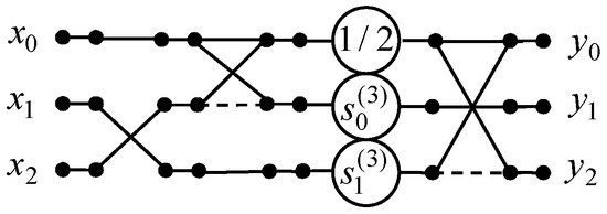
Figure 1.
The data flow graph of the three-point DKT algorithm.
3.2. Algorithm for the 4-Point DKT
Let us present the 4-point DKT as a matrix-vector product:
where , , with = 0.3536 and = 0.6124.
We apply the structural approach [33,34] to factorize the matrix . In this way, the order of the columns and rows of the matrix was altered with the permutations and . The permutation matrices are and .
It can be noted that the resulting matrix can be represented as where and . The matrices , , and are factorized as follows [33]:
where , .
As a result, we have yielded the following factorization of the 4-point DKT matrix:
where ,, , , , , , , , =.
A data flow graph of the proposed four-point DKT algorithm is constructed in Figure 2. Note that the initial 4-point DKT requires 16 multiplications and 12 additions. With the proposed 4-point DKT algorithm, the number of multiplications can be reduced from 16 to 6. The number of additions can be reduced from 12 to 10.
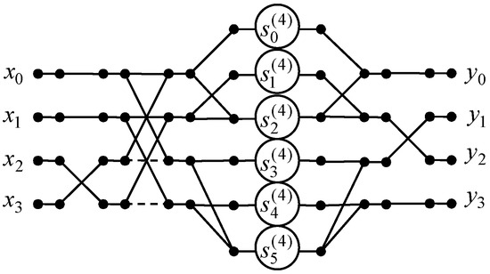
Figure 2.
The data flow graph of the 4-point DKT algorithm.
3.3. Algorithm for the 5-Point DKT
Next, we design the algorithm for the 5-point DKT which is expressed as follows:
where , , with = 0.25; = 0.5; = 0.6124.
Let us change the order of columns of the matrix according to the permutation . Then we obtain the matrix with the permutation matrix .
To construct the factorization of the matrix , we note that after the permutation of , we have obtained pairs of repeating elements in the first four columns. These elements may differ in sign. We construct the butterfly modules for these columns using the matrix . In place of the fifth column, we include a unit on the diagonal of the matrix .
Next, we form a diagonal matrix , where , from the repeating elements of the columns of the matrix . The final matrix included in the factorization connects output variables to linear combinations of input values. Thus, we obtained the following factorization of the 5-point DKT matrix:
where .
We show a data flow graph of the proposed 5-point DKT algorithm in Figure 3. The initial 5-point DKT requires 4 multiplications, 16 additions, and 21 shifts because four entries of the transform matrix are equal to zero. We have taken into account that multiplication by = 0.25 requires two shifts and multiplication by = 0.5 requires one shift. The developed 5-point DKT algorithm reduces the number of multiplication to 2 because . The number of additions is decreased from 16 to 12, and 6 shifts are required.
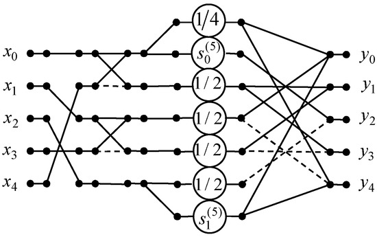
Figure 3.
The data flow graph of the 5-point DKT algorithm.
3.4. Algorithm for the 6-Point DKT
Let us obtain the algorithm for the 6-point DKT, which is expressed as follows:
where , , with = 0.1768, = 0.3953, = 0.5590, = 0.5303, = 0.25, = 0.3536.
The columns and rows of the matrix are permutated according to the permutations and which are defined in the following form: and .
Then the matrix is represented as . The matrices and are the permutation matrices.
The resulting matrix can be represented as where and . We change the order of the columns of the matrix and obtain the matrix . Next, we swap the second and third columns of the matrix and yield the matrix .
Let us extract the submatrices and from the matrices and , respectively. Then the matrices , , and are factorized as follows [34]:
where .
Let us denote the scaling factors as , , , , , and form the diagonal matrix . Further, we add matrices from decomposition (14) to the left of the diagonal matrices into the matrix , and to the right of the diagonal matrices into the matrices ,, where , , and are defined as follows:
Combining the matrices , , , and we obtain the matrix factorization for the 6-point DKT:
where .
We present the data flow graph for the 6-point DKT algorithm in Figure 4. It should be noted that the initial 6-point DKT requires 28 multiplications, 30 additions, and 16 shifts because = 0.25, and we have 8 such entries in the 6-point DKT matrix . The developed 6-point DKT algorithm reduces the number of multiplications to 12. The number of additions has decreased from 30 to 20, and 8 shifts are required.
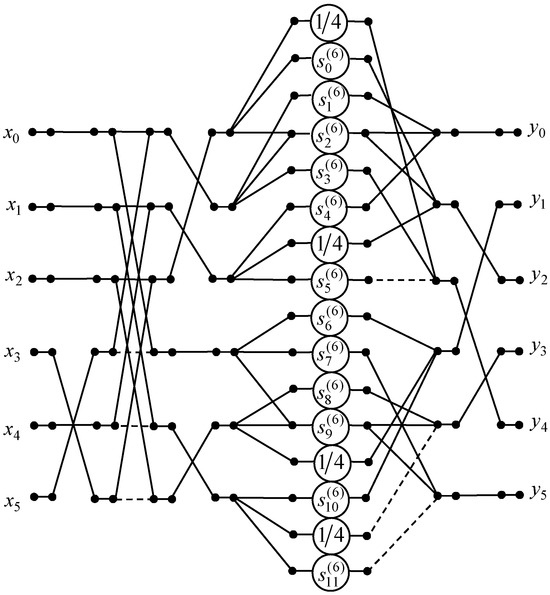
Figure 4.
The data flow graph of the six-point DKT algorithm.
3.5. Algorithm for the 7-Point DKT
Let us construct the algorithm for 7-point DKT based on the following expression:
where , , with = 0.1250, = 0.3062, = 0.4841, = 0.5590, = 0.5, = 0.3953, = 0.4330. We change the order of columns of the matrix with the permutation . As a result, the matrix and the permutation matrix are obtained:
The factorization of the matrix was introduced similarly to the factorization of the matrix [35]. This matrix contains pairs of repeating elements in adjacent columns, and these elements may differ in sign. This structure allows us to extract the butterfly modules using the matrix . The values of the repeating elements were entered into a diagonal matrix , where , , , , , . This matrix was linked to the butterfly modules using the matrix . To calculate the output variables, the matrix
was formed. As a result, we have the factorization:
The calculation of the 7-point DKT with the matrix-vector product requires 40 multiplications, 37 additions, and 4 shifts because five elements of the matrix are zeros. Four elements of this matrix are equal to 0.5, and multiplication by these elements can be implemented using shifts.
The repeated elements of the matrix allow the designing of the data flow graph for the 7-point DKT algorithm presented in Figure 5. This algorithm reduces the number of multiplications from 40 to 12. The number of additions and shifts can be decreased from 37 to 23 and from 4 to 1, respectively.
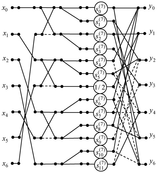
Figure 5.
The data flow graph of the 7-point DKT algorithm.
3.6. Algorithm for the 8-Point DKT
To design the algorithm for 8-point DKT we express this transform as a matrix-vector product:
where , , with = 0.0884, = 0.2339, = 0.4050, = 0.5229, = 0.4419, = 0.4593, = 0.1976, = 0.3423, = 0.2652.
To alter the order of rows and columns of the matrix we define the permutation and . As a result, we obtain the permutation matrices and :
The resulting matrix matches the template which is factorized as follows [33]:
where and .
Let us consider the matrix which matches the template after the permutation of columns with the matrix . The obtained matrix is decomposed as [33]:
where , , , , , and . The matrix , , , and can be represented as follows [33]:
We alter the order of the columns of the matrix with the permutation . The signs of the entries in the third and fourth columns of the resulting matrix were then changed. The obtained matrix is also factorized with Equation (22).
Let us add the matrices from decomposition (21) to the expressions and . After applying the decomposition (22) to the matrices and we join matrices to the left of the diagonal matrix into the matrix . Also, we add matrices to the right of the diagonal matrix into the matrix .
Combining the matrices , , , and we obtain the matrix factorization for the 8-point DKT:
where , , , , , , , , , , . The additional permutation matrix is introduced as a direct sum of the two matrices: and .
Based on the obtained factorization of the matrix, the algorithm of the 8-point DKT calculation is proposed. The data flow graph of this algorithm is presented in Figure 6. The computing of the 8-point DKT with the proposed algorithm can reduce the required number of multiplications from 64 to 26. The number of additions decreased from 56 to 38.
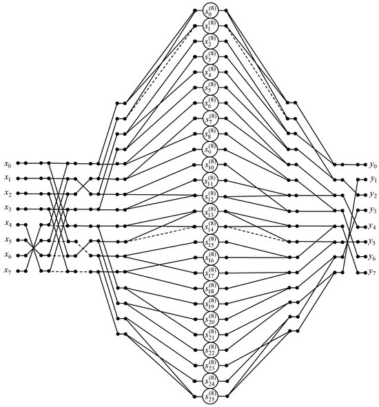
Figure 6.
The data flow graph of the 8-point DKT algorithm.
3.7. Generalization of the Proposed Algorithms
Considering the symmetry of orthogonal Krawtchouk polynomials, we propose a generalization of the developed DKT algorithms for short-length input sequences when N is greater than 8. Taking into account Equation (5), we consider the cases of odd and even lengths of input signals separately to obtain the fast N-point DKT algorithms.
Let us suppose that N is even and define the permutation of columns of the DKT matrix similarly with [35] as:
The corresponding permutation matrix we denote as . Next, the inputs after the permutations are pairwise combined into butterfly modules by multiplying by the matrix where is included in the direct sum N/2 times. Further, the outputs of each butterfly module are transmitted to a layer of multipliers using the matrix where is included in the direct sum N times. The layer of multipliers is presented by a diagonal matrix . We include into the diagonal matrix the elements of the original DKT matrix located in the first N rows of this matrix and the first N/2 columns:
In sum, the output variables of the N-point DKT were obtained as follows:
The matrix in the factorization (26) establishes a link between the output variables and linear combinations of the input values.
Let us consider an odd N. In this case the order of the columns of the DKT matrix is changed using the permutation
where denotes the floor of . The symmetry of Krawtchouk polynomials is considered once again. By (27) we introduce the permutation matrix . As in the previous case, we pairwise combine the inputs after the permutations into butterfly modules by multiplying by the matrix where is included in the direct sum times.
Next, we consider two cases of value . The first case is that is an even number. Then N = 7, 11, 15, …, and the outputs of each butterfly module are transmitted to a layer of multipliers using the matrix where n = (N + 1)/4, and is included in the direct sum times. The second case is that is an odd number. Then N = 9, 13, 17, …, and the outputs of each butterfly module are transmitted to a layer of multipliers using the matrix where m = (N + 3)/4, l = (N 1)/4, is included in the direct sum times.
The layer of multipliers is presented by a diagonal matrix . In the diagonal matrix we expand by columns the elements of the original DKT matrix located in the first rows of this matrix and the first columns:
As a result, the output variables of the N-point DKT were obtained as follows:
where is the matrix that was included in the factorization to establish a correspondence between the outputs and linear combinations of the values of the inputs. The matrix is sparse and has a complex structure similar to that of the matrices and . One can see that entries equal to one or minus one form the diamond structure in such matrices.
We note that when constructing the generalized algorithm, it was not taken into account that there may be zeros among the entries of the diagonal matrix. Then the corresponding paths on the data flow graph must be deleted. As a result, the resulting graph will have a simpler structure.
4. Results
Each proposed algorithm has been implemented in the MATLAB environment, and the correctness of the algorithm is verified. The research was performed using an Intel Core i5-7400 processor (Intel, Santa Clara, CA, USA), 3 GHz CPU, 16 GB memory, Windows 10 operating system, 64-bit. To test the designed algorithms, we compare the number of arithmetic operations for computing the DKT with direct matrix-vector products and with the developed algorithms. Initially, the DKT matrices were obtained by applying Equations (6), (8), (11), (13), (17) and (19) for N ranging from 3 to 8. Next, the DKT matrix factorizations were calculated with the expressions (7), (10), (12), (16), (18), and (23). We determined the correctness of the proposed algorithms, establishing the coincidence of the entries of DKT matrices and the entries of the products of the matrices included in the factorizations of the DKT matrices for the same N.
Additionally, we evaluated the number of arithmetic operations involved in the designed algorithms. The results are presented in Table 1. The percentage reduction in the number of operations is indicated in parentheses, compared to the direct method. It can be seen from Table 1 that for values of N ranging from 3 to 8, the number of multiplications, additions, and shifts is reduced by an average of 58%, 27%, and 68%, respectively.

Table 1.
The number of additions, multiplications, and shifts in the constructed DKT algorithms and the direct matrix-vector products.
5. Discussion of Computational Complexity
In Table 2, we have shown the number of additions, shifts, and multiplications for the DKT algorithms obtained based on the symmetry of Krawtchouk polynomials and with the structural approach. The results in Table 2 revealed that the number of additions is less by 11–28% for algorithms developed based on the symmetry of Krawtchouk polynomials. The algorithms designed with the structural approach required fewer multiplications by 14–25%. Applying the structural approach, we actually replace several multiplications (their number depends on N) with the same number of additions, which are less time-consuming and resource-intensive.
Table 2.
The number of additions, multiplications, and shifts in the constructed DKT algorithms based on a structural approach and taking into account the symmetry of Krawtchouk polynomials.
In addition, in Table 2, we provide estimates of the number of arithmetic operations for generalization the presented algorithms for even and odd N. The direct matrix-vector product requires multiplications and N(N − 1) additions. Then we obtain that the number of multiplications can be reduced in two times.
Memory consumption results for the proposed DKT algorithms are shown in Figure 7. We have calculated the number of memory cells required for the algorithms presented in Section 3 using the designed pseudocodes. These pseudocodes are shown in Appendix A. Our solutions use 34% more memory than the direct matrix-vector product. We averaged this characteristic over the input sizes ranging from 4 to 8.
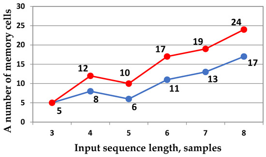
Figure 7.
Diagram of the memory consumption for the DKT, which is implemented via a direct matrix-vector product (blue line) and the proposed algorithms (red line).
It should be noted that memory consumption depends heavily on implementation methods, platform, and the designer’s expertise, unlike more objective measures of arithmetic complexity. The constructed DKT algorithms support software implementation, which may vary in memory usage, time delays, and required resources. The same memory cells can be reused on different algorithm stages if possible. Moreover, the developed solutions can be implemented sequentially, in parallel, or in combination, affecting result latency. Thus, the evaluation of the efficiency of memory use is subjective. Consequently, arithmetic complexity remains the most reliable measure of the efficiency of the proposed algorithms since implementation details are not considered.
6. Conclusions
In this article, we have developed algorithms for the DKT with a fixed p equal to 0.5, applying the structural approach. It is supposed that the length N of the input sequence is in the range of 3 to 8. Compared to the direct matrix-vector product, the obtained algorithms reduce the number of multiplications, additions, and shifts by approximately 58%, 27%, and 68%, respectively. We averaged these characteristics over the considered input sizes (from 3 to 8).
The designed algorithms were represented using data flow graphs. One unquestionable benefit of the suggested solutions is that each designed data flow graph’s critical path only has one multiplication. It is well known that additional data processing problems arise due to the doubling of the operand format with each subsequent multiplication if the critical path in the algorithm’s data flow graph contains more than one multiplication. Our algorithms do not have this problem.
We have generalized the obtained algorithms for small-sized DKT to the case of long input sequences. A matrix factorization of each proposed solution is derived based on the symmetry property of the Krawtchouk polynomials. Each such factorization has been constructed using sparse matrices. Based on the matrix factorization for a specific signal length N, the DKT algorithm can be represented by a data flow graph. The number of arithmetic operations of the generalized algorithms was compared to that of the algorithms derived from the structural approach. As a result, the universal and simpler solution may be followed by a little decrease in computational efficiency.
The developed fast DKT algorithms do not directly affect accuracy in application contexts. This is because the proposed algorithms reduce the number of arithmetic operations required to compute the matrix-vector product, but do not alter its values. For example, in image feature extraction with varying image resolutions, accuracy significantly depends on the methods used to calculate the elements of the transform matrix and on data preprocessing. The specific algorithms presented do not impact this accuracy.
However, the proposed algorithms have certain limitations. First, the structural approach is better suited for constructing fast algorithms for short data sequences. Identifying the structure of transform matrices becomes more challenging with longer sequences. To address this, we have developed the generalization of the proposed DKT algorithms in Section 3.7. Second, the efficiency of synthesizing the presented fast algorithms relies heavily on the structural properties of the transform matrices. Specifically, it depends on how effectively these matrices can be transformed to align their block structure with the matrix patterns described in [33]. The symmetry of the Krawtchouk polynomials assumes a specific structure of the DKT matrices. This enabled us to develop a generalization of the fast DKT algorithms for input sequence lengths exceeding 8. Future research may focus on applying the proposed fast DKT algorithms and their generalization in image inpainting in the spectral domain using convolutional neural networks [36]. In quantum watermarking schemes, orthogonal transforms can decompose digital images into basis items or basis images [37]. These basis images can have simple quantum analogs that represent quantum operators describing transitions between quantum states. This property of orthogonal transforms allows watermark embedding in the frequency domain, where watermark bits or quantum watermark information are embedded into transformed components rather than directly into pixels, enhancing security [37].
Another promising area for future research is the development of fast DKT algorithms for long input sequences, constructing a fast orthogonal projection of the DKT using the Kronecker product, which generates large orthogonal matrices from smaller ones [25,26]. This enables the adaptation of DKT algorithms designed for short-length sequences to process long-length sequences. In this way, the computational complexity of the DKT can be significantly reduced, enhancing its efficiency for practical applications [36,37].
Author Contributions
Conceptualization, A.C.; methodology, A.C. and M.P.; software, M.P.; validation, A.C., M.P. and J.P.P.; formal analysis, A.C., M.P. and J.P.P.; investigation, M.P.; writing—original draft preparation, M.P. and A.C.; writing—review and editing, A.C., M.P. and J.P.P.; supervision, A.C. All authors have read and agreed to the published version of the manuscript.
Funding
This research received no external funding.
Data Availability Statement
Data are contained within the article.
Conflicts of Interest
The authors declare no conflicts of interest. The funders had no role in the design of the study; in the collection, analyses, or interpretation of data; in the writing of the manuscript; or in the decision to publish the results.
Appendix A
The appendix presents the pseudocode of the proposed fast DKT algorithms. These pseudocodes were used in Section 4 to calculate the number of memory cells required for the algorithms presented in Section 3. To save the memory cells required for implementing the constructed algorithms, we reuse variables and specify which variables must be output and in which order. Thus, in Table A1, the pseudocode of the proposed 3-point DKT algorithm is presented. The inputs of the pseudocode are and Because the scaling factors are similar for this algorithm (), we use only to construct the pseudocode. We reuse variables; then is an additional variable and the outputs of the pseudocode are and
Table A1.
The pseudocode for the constructed fast DKT algorithm for N = 3 with variable reuse.
Table A1.
The pseudocode for the constructed fast DKT algorithm for N = 3 with variable reuse.
| Step 1 | Step 2 |
|---|---|
| , ; |
We present the pseudocode for the developed 4-point DKT algorithm in Table A2. The inputs of the pseudocode are and We use only scaling factors , , , and to design the pseudocode. This is due to the following relations between the scaling factors: , . We reuse variables; additional variables are and The outputs of the pseudocode are and
Table A2.
The pseudocode for the developed fast 4-point DKT algorithm with variable reuse.
Table A2.
The pseudocode for the developed fast 4-point DKT algorithm with variable reuse.
| Step 1 | Step 2 | Step 3 |
|---|---|---|
| , , ; | , , | , |
The pseudocode for the designed 5-point DKT algorithm is shown in Table A3. The inputs of the pseudocode are and We use only scaling factor because . The outputs of the pseudocode are and due to variable reusing. Variables and are additional.
Table A3.
The pseudocode for the designed 5-point DKT algorithm with variable reuse.
Table A3.
The pseudocode for the designed 5-point DKT algorithm with variable reuse.
| Step 1 | Step 2 | Step 3 |
|---|---|---|
| , , ; | , , , ; | , . |
In Table A4, the pseudocode of the proposed 6-point DKT algorithm is presented. The inputs of the pseudocode are and We use only scaling factors , , , , and because , , , , . We reuse variables. So, the outputs of the pseudocode are and Variables and are additional.
Table A4.
The pseudocode for the developed 6-point DKT algorithm with variable reuse.
Table A4.
The pseudocode for the developed 6-point DKT algorithm with variable reuse.
| Step 1 | Step 2 | Step 3 |
|---|---|---|
| , , ,; |
In Table A5, the pseudocode of the constructed 7-point DKT algorithm is shown. The inputs of the pseudocode are and We use only scaling factors , , , , , and because , , , , , and . We reuse variables. So, the outputs of the pseudocode are and
Table A5.
The pseudocode for the designed 7-point DKT algorithm with variable reuse.
Table A5.
The pseudocode for the designed 7-point DKT algorithm with variable reuse.
| Step 1 | Step 2 | Step 3 |
|---|---|---|
| , , ,; | . |
In Table A6, the pseudocode of the constructed 8-point DKT algorithm is presented. The inputs of the pseudocode are , and We use scaling factors , , , , , , , , because , , , , , , , , . We reuse variables. So, the outputs of the pseudocode are and
Table A6.
The pseudocode for the constructed 8-point DKT algorithm with variable reuse.
Table A6.
The pseudocode for the constructed 8-point DKT algorithm with variable reuse.
| Step 1 | Step 2 | Step 3 | Step 4 | Step 5 |
|---|---|---|---|---|
| , , , , ; |
References
- Flusser, J.; Suk, T.; Zitová, B. 2D and 3D Image Analysis by Moments; John Wiley & Sons: Hoboken, NJ, USA, 2016. [Google Scholar]
- Yang, L.; Liu, X.; Hu, Z. Advance and prospect of discrete Tchebichef transform and its application. In Proceedings of the 2020 IEEE 4th Information Technology, Networking, Electronic and Automation Control Conference (ITNEC), Chongqing, China, 12–14 June 2020. [Google Scholar]
- Mefoued, A.; Kouadria, N.; Harize, S.; Doghmane, N. Improved discrete Tchebichef transform approximations for efficient image compression. J. Real-Time Image Process. 2023, 21, 12. [Google Scholar] [CrossRef]
- Ke, W.; Chan, K.-H. A multilayer CARU framework to obtain probability distribution for paragraph-based sentiment analysis. Appl. Sci. 2021, 11, 11344. [Google Scholar] [CrossRef]
- Tahiri, M.A.; Amakdouf, H.; El Mallahi, M.; Qjidaa, H. Optimized quaternion radial Hahn moments application to deep learning for the classification of diabetic retinopathy. Multimed Tools Appl. 2023, 82, 46217–46240. [Google Scholar] [CrossRef]
- Younsi, M.; Diaf, M.; Siarry, P. Comparative study of orthogonal moments for human postures recognition. Eng. Appl. Artif. Intell. 2023, 120, 105855. [Google Scholar] [CrossRef]
- Chiang, A.; Liao, S. Image analysis with Legendre moment descriptors. J. Comput. Sci. 2015, 11, 127–136. [Google Scholar] [CrossRef]
- Camacho-Bello, C. Exact Legendre–Fourier moments in improved polar pixels configuration for image analysis. IET Image Process. 2018, 13, 118–124. [Google Scholar] [CrossRef]
- Asli, B.H.S.; Flusser, J. Fast computation of Krawtchouk moments. Inf. Sci. 2014, 288, 73–86. [Google Scholar] [CrossRef]
- Venkataramana, A.; Raj, P.A. Image watermarking using Krawtchouk moments. In Proceedings of the 2007 International Conference on Computing: Theory and Applications (ICCTA’07), Kolkata, India, 5–7 March 2007; pp. 676–680. [Google Scholar]
- Papakostas, G.A.; Tsougenis, E.D.; Koulouriotis, D.E. Near optimum local image watermarking using Krawtchouk moments. In Proceedings of the 2010 IEEE International Conference on Imaging Systems and Techniques, Thessaloniki, Greece, 1–2 July 2010; pp. 464–467. [Google Scholar]
- Yamni, M.; Karmouni, H.; Daoui, A.; Sayyouri, M.; Qjidaa, H. Blind image zero-watermarking algorithm based on radial Krawtchouk moments and chaotic system. In Proceedings of the 2020 International Conference on Intelligent Systems and Computer Vision (ISCV), Fez, Morocco, 9–11 June 2020; pp. 1–7. [Google Scholar]
- Zhang, L.; Xiao, W.; Qian, G.; Ji, Z. Rotation, scaling, and translation invariant local watermarking technique with Krawtchouk moments. Chin. Opt. Lett. 2007, 5, 21–24. [Google Scholar]
- Yap, P.-T.; Paramesran, R.; Ong, S.-H. Image analysis by Krawtchouk moments. IEEE Trans. Image Process. 2003, 12, 1367–1377. [Google Scholar] [CrossRef]
- Yap, P.T.; Raveendran, P.; Ong, S.H. Krawtchouk moments as a new set of discrete orthogonal moments for image reconstruction. In Proceedings of the 2002 International Joint Conference on Neural Networks, IJCNN’02 (Cat. No.02CH37290), Honolulu, HI, USA, 12–17 May 2002; Volume 1, pp. 908–912. [Google Scholar]
- Karmouni, H.; Jahid, T.; Lakhili, Z.; Hmimid, A.; Sayyouri, M.; Qjidaa, H.; Rezzouk, A. Image reconstruction by Krawtchouk moments via digital filter. In Proceedings of the International Conference on Intelligent Systems and Computer Vision (ISCV), Fez, Morocco, 17–19 April 2017; pp. 1–7. [Google Scholar]
- Mesbah, A.; El Mallahi, M.; Lakhili, Z.; Qjidaa, H.; Berrahou, A. Fast and accurate algorithm for 3D local object reconstruction using Krawtchouk moments. In Proceedings of the 2016 5th International Conference on Multimedia Computing and Systems (ICMCS), Marrakech, Morocco, 29 September–1 October 2016; pp. 1–6. [Google Scholar]
- Rani, J.S.; Devaraj, D. Face recognition using Krawtchouk moment. Sadhana 2012, 37, 441–460. [Google Scholar] [CrossRef]
- Rivero-Castillo, D.; Pijeira, H.; Assunçao, P. Edge detection based on Krawtchouk polynomials. J. Comput. Appl. Math. 2015, 284, 244–250. [Google Scholar] [CrossRef]
- Yamni, M.; Daoui, A.; Pławiak, P.; Mao, H.; Alfarraj, O.; El-Latif, A.A.A. A novel 3D reversible data hiding scheme based on integer–reversible Krawtchouk transform for IoMT. Sensors 2023, 23, 7914. [Google Scholar] [CrossRef] [PubMed]
- Chen, Y.; Yao, X.-R.; Zhao, Q.; Liu, S.; Liu, X.-F.; Wang, C.; Zhai, G.-J. Single-pixel compressive imaging based on the transformation of discrete orthogonal Krawtchouk moments. Opt. Express 2019, 27, 29838–29853. [Google Scholar] [CrossRef] [PubMed]
- Zhao, W.; Gao, L.; Zhai, A.; Wang, D. Comparison of common algorithms for single-pixel imaging via compressed sensing. Sensors 2023, 23, 4678. [Google Scholar] [CrossRef]
- Honarvar Shakibaei Asli, B.; Horri Rezaei, M. Four-term recurrence for fast Krawtchouk moments using Clenshaw algorithm. Electronics 2023, 12, 1834. [Google Scholar] [CrossRef]
- Abdulhussain, S.H.; Ramli, A.R.; Al-Haddad, S.A.R.; Mahmmod, B.M.; Jassim, W.A. Fast recursive computation of Krawtchouk polynomials. J. Math. Imaging Vis. 2018, 60, 285–303. [Google Scholar] [CrossRef]
- Zhang, X.; Yu, F.X.; Guo, R.; Kumar, S.; Wang, S.; Chang, S.-F. Fast orthogonal projection based on Kronecker product. In Proceedings of the 2015 IEEE International Conference on Computer Vision (ICCV), Santiago, Chile, 7–13 December 2015; pp. 2929–2937. [Google Scholar]
- Majorkowska-Mech, D.; Cariow, A. Discrete pseudo-fractional Fourier transform and its fast algorithm. Electronics 2021, 10, 2145. [Google Scholar] [CrossRef]
- Mahmmod, B.M.; Abdul-Hadi, A.M.; Abdulhussain, S.H.; Hussien, A. On computational aspects of Krawtchouk polynomials for high orders. J. Imaging 2020, 6, 81. [Google Scholar] [CrossRef]
- Al-Utaibi, K.A.; Abdulhussain, S.H.; Mahmmod, B.M.; Naser, M.A.; Alsabah, M.; Sait, S.M. Reliable recurrence algorithm for high-order Krawtchouk polynomials. Entropy 2021, 23, 1162. [Google Scholar] [CrossRef]
- Venkataramana, A.; Raj, P.A. Recursive computation of forward Krawtchouk moment transform using Clenshaw’s recurrence formula. In Proceedings of the 2011 Third National Conference on Computer Vision, Pattern Recognition, Image Processing and Graphics, Hubli, India, 15–17 December 2011; pp. 200–203. [Google Scholar]
- Karampasis, N.D.; Spiliotis, I.M.; Boutalis, Y.S. Real-time computation of Krawtchouk moments on gray images using block representation. SN Comput. Sci. 2021, 2, 124. [Google Scholar] [CrossRef]
- Mesbah, A.; El Mallahi, M.; El Fadili, H.; Zenkouar, K.; Berrahou, A.; Qjidaa, H. An algorithm for fast computation of 3D Krawtchouk moments for volumetric image reconstruction. In Proceedings of the Mediterranean Conference on Information & Communication Technologies 2015 (MedCT 2015), Saïdia, Morocco, 7–9 May 2015; El Oualkadi, A., Choubani, F., El Moussati, A., Eds.; Lecture Notes in Electrical Engineering. Springer: Cham, Switzerland, 2015; Volume 380. [Google Scholar]
- Wu, J.S.; Yang, C.F.; Shu, H.Z.; Wang, L.; Senhadji, L. A fast algorithm for the 4x4 discrete Krawtchouk transform. In Proceedings of the 2014 International Symposium on Information Technology (ISIT 2014), Dalian, China, 14–16 October 2014; pp. 23–28. [Google Scholar]
- Andreatto, B.; Cariow, A. Automatic generation of fast algorithms for matrix-vector multiplication. Int. J. Comput. Math. 2017, 95, 626–644. [Google Scholar] [CrossRef]
- Polyakova, M.; Witenberg, A.; Cariow, A. The fast type-IV discrete sine transform algorithms for short-length input sequences. Bull. Pol. Acad. Sci. Tech. Sci. 2025, 73, e153827. [Google Scholar] [CrossRef]
- Cariow, A.; Polyakova, M. The fast discrete Tchebichef transform algorithms for short-length input sequences. Signals 2025, 6, 23. [Google Scholar] [CrossRef]
- Kolodochka, D.; Polyakova, M.; Rogachko, V. Prediction the accuracy of image inpainting using texture descriptors. Radio Electron. Comput. Sci. Manag. 2025, 2, 56–67. [Google Scholar] [CrossRef]
- Xing, Z.; Lam, C.-T.; Yuan, X.; Im, S.-K.; Machado, P. MMQW: Multi-Modal Quantum Watermarking Scheme. IEEE Trans. Inf. Forensics Secur. 2024, 19, 5181–5195. [Google Scholar] [CrossRef]
Disclaimer/Publisher’s Note: The statements, opinions and data contained in all publications are solely those of the individual author(s) and contributor(s) and not of MDPI and/or the editor(s). MDPI and/or the editor(s) disclaim responsibility for any injury to people or property resulting from any ideas, methods, instructions or products referred to in the content. |
© 2025 by the authors. Licensee MDPI, Basel, Switzerland. This article is an open access article distributed under the terms and conditions of the Creative Commons Attribution (CC BY) license (https://creativecommons.org/licenses/by/4.0/).