Abstract
Industrial control systems (ICSs) face escalating security challenges due to evolving cyber threats and the inherent limitations of traditional intrusion detection methods, which fail to adequately model spatiotemporal dependencies or interpret complex protocol semantics. To address these gaps, this paper proposes DLG–IDS—a lightweight intrusion detection framework that innovatively integrates dynamic graph construction for capturing real–time device interactions and logical control relationships from traffic, LLM–driven semantic enhancement to extract fine–grained embeddings from graphs, and a spatio–temporal graph neural network (STGNN) optimized via sparse attention and local window Transformers to minimize computational overhead. Evaluations on SWaT and SBFF datasets demonstrate the framework’s superiority, achieving a state–of–the–art accuracy of 0.986 while reducing latency by 53.2% compared to baseline models. Ablation studies further validate the critical contributions of semantic fusion, sparse topology modeling, and localized temporal attention. The proposed solution establishes a robust, real–time detection mechanism tailored for resource–constrained industrial environments, effectively balancing high accuracy with operational efficiency.
1. Introduction
The rapid evolution of industrial control systems (ICSs) has led to their widespread adoption in critical infrastructure sectors such as energy, manufacturing, and transportation. While these systems have significantly enhanced operational efficiency and automation, they have also become prime targets for cyber–attacks. The interconnected nature of modern ICSs, often referred to as the Industrial Internet of Things (IIoT), has introduced new vulnerabilities that can be exploited by malicious actors. Consequently, the detection of anomalous network traffic in industrial control networks (ICNs) has emerged as a critical research area to ensure the security and reliability of these systems.
Traditional network intrusion detection systems (NIDSs) have primarily relied on signature–based methods [1] and statistical anomaly detection techniques [2]. However, these approaches often fall short in addressing the unique challenges posed by ICNs. The highly dynamic and heterogeneous nature of industrial network traffic, coupled with the stringent real–time requirements of ICSs, necessitates the development of more sophisticated detection mechanisms. Moreover, the increasing complexity of cyber–attacks, which often involve multi–stage and coordinated activities, further underscores the limitations of conventional methods.
In recent years, graph neural networks (GNNs) have gained attention for their ability to model complex relationships in structured data by representing network traffic as graphs [3], where nodes correspond to devices and edges represent communication patterns. This allows GNNs to capture spatial and temporal dependencies, making them well–suited for ICN anomaly detection. However, most existing GNN–based studies focus on either spatial [4] or temporal [5] aspects in isolation, rather than integrating both dimensions. Additionally, they struggle with the unique characteristics of ICN traffic, such as periodicity, high dimensionality, and the presence of both continuous and discrete data. Static graph models, for example, cannot accommodate dynamic changes in network topology due to device additions or removals, while dynamic graph approaches often face high computational complexity that hinders real–time performance.
Spatio–temporal graph neural networks (STGNNs) have advanced spatiotemporal modeling but still have critical limitations. They typically treat protocol fields as discrete symbols or numerical features [6], lacking in–depth analysis of operational intent—for instance, failing to distinguish between legitimate “write register” commands and malicious parameter tampering. They also underutilize multi–modal data, missing opportunities to leverage rich semantic information. Furthermore, the computational complexity of STGNNs conflicts with the resource constraints of industrial edge devices, making it difficult to meet real–time response requirements.
Large language models (LLMs) offer potential for addressing these semantic gaps through their strong natural language understanding capabilities. However, existing work isolates LLMs in text processing or rule generation [7], rather than embedding them into spatio–temporal traffic modeling. For example, while LLMs have been used to parse protocol fields or generate attack scenarios, they are not integrated with dynamic graph structures, leaving a disconnect between semantic context and network behavior that hinders detection of covert attacks like parameter tampering within compliant protocol frames.
To address these interconnected limitations, this paper proposes DLG–IDS—a lightweight intrusion detection framework that integrates the following three core innovations:
- A dynamic graph construction method that combines real–time communication patterns and logical control dependencies into a unified graph structure, overcoming the static nature of traditional graph models and capturing spatiotemporal dynamics in industrial networks.
- LLM–driven semantic enhancement that generates fine–grained semantic embeddings from protocol content and device logs, aligning these with network traffic statistical features through cross–modal attention to bridge the gap in protocol intent understanding.
- A lightweight STGNN optimized with sparse graph attention and local window Transformers, which reduces computational complexity from quadratic to linear while preserving the ability to model spatiotemporal dependencies, addressing the conflict between resource constraints and real–time requirements.
To evaluate the effectiveness of the algorithm, we conducted extensive experiments on different datasets. The results demonstrate that the proposed detection method outperforms traditional methods and state–of–the–art deep learning models in terms of detection accuracy, false positive rate, and computational efficiency. We also provide a detailed analysis of the model’s performance under different attack scenarios, highlighting its robustness and adaptability to various types of anomalies.
The rest of this paper is organized as follows: Section 2 reviews related work on network intrusion detection. Section 3 presents the detailed methodology of our DLG–IDS algorithm, including the dynamic graph construction, the integration of LLMs, and the neural network architecture. Section 4 introduces the experimental setup and provides the evaluation results. Finally, Section 5 concludes the paper and discusses future research directions.
2. Related Work
2.1. Traditional Industrial Network Anomaly Detection Methods
Traditional industrial network anomaly detection methods can be roughly divided into three categories: rule–based methods, statistical analysis methods, and early machine learning methods. These approaches played an important role in the early stages of industrial network security, but as the complexity of attacks has increased, their limitations have gradually become apparent.
Rule–based methods match anomaly patterns in network traffic based on predefined rule libraries, typically focusing on the legitimate operation ranges of specific industrial protocols, such as Modbus or DNP3, through hard–coded constraints. Cheung [8] proposed a state machine model based on the Modbus protocol, defining legitimate function codes and register address ranges. If a function code exceeds the valid range or there is illegal register access, an alert is triggered. Hadžiosmanović et al. [9] designed a whitelist system for industrial protocols, only allowing communication between pre–authorized devices, such as fixed IP port interactions between PLCs and SCADA systems, blocking unauthorized connection attempts.
Rule–based methods have clear logical structures that are easy for operations staff to understand, and they have low computational overhead, making them suitable for resource–constrained industrial devices. However, the rule library requires manual updates, and static rules struggle to cope with zero–day attacks or protocol variations. Additionally, false positive rates are high, as temporary configuration changes in normal operations may be misidentified as anomalies. On the other hand, due to limited protocol coverage, defining rules for proprietary protocols depends on reverse engineering, which is time–consuming and prone to errors.
Statistical analysis methods detect abnormal behaviors by modeling the distribution of features such as packet length, frequency, and periodicity in normal traffic and identifying deviations from the normal baseline. The operation of industrial devices tends to follow a certain periodicity, which is reflected in industrial traffic as well. Lai [10] utilized an Autoregressive Integrated Moving Average (ARIMA) model to model the periodicity of industrial traffic and detect abnormal fluctuations in traffic intervals. Ujjan [11] proposed an anomaly index based on information entropy. Since attack traffic often targets a small number of ports, DDoS attacks lead to a sharp drop in the entropy value of the target port. By calculating the entropy changes in features like source IP and target port within a specific time window, attacks can be detected.
Statistical analysis methods automatically learn normal patterns through data–driven approaches without requiring prior knowledge, making them partially adaptive to dynamic environments. However, their detection performance highly depends on manually selected statistical indicators, and univariate statistical methods tend to overlook the interaction relationships between devices.
Early machine learning methods primarily utilized supervised or semi–supervised learning algorithms, relying on feature engineering to classify extracted traffic attributes. Wang [12] extracted 40–dimensional features such as the number of connections per second and the distribution of TCP flags from industrial control traffic, and trained a CNN–BiLSTM classifier to distinguish normal traffic from ARP virus attacks. Dakheel [13] combined traffic statistical features with protocol semantics to use Random Forest (RF) for detecting parameter injection attacks, achieving 92% accuracy on a natural gas pipeline dataset. Ridi [14] employed Hidden Markov Models (HMMs) to model the state transition sequences of industrial devices, identifying abnormal state shifts.
Machine learning methods reduce the workload of manually defining rules and enhance the automation of anomaly detection. However, feature engineering still faces bottlenecks. The diversity and proprietary nature of industrial protocols make it difficult to build a universal feature set. Furthermore, supervised learning relies on a large number of labeled samples, but due to the rarity and sensitivity of actual industrial attack cases, obtaining sufficient data is challenging. Static models also struggle to adapt to the dynamic topology of industrial control systems, as industrial network devices may be dynamically added or removed based on production tasks, leading to feature distribution shifts.
Traditional methods have laid an important foundation for industrial network anomaly detection, but their core issues lie in their reliance on rules, feature engineering, and other manual prior knowledge, as well as fragmented detection logic. These methods tend to overlook the spatio–temporal correlations between devices. Given these limitations, it is necessary to explore other models or detection methods that are more suitable for the dynamic and complex nature of industrial networks.
2.2. Traffic Modeling Method Based on Graph Neural Networks
Traffic modeling methods based on graph neural networks (GNNs) have made significant progress in the field of anomaly detection in recent years, particularly in capturing the complex spatio–temporal dependencies between devices in a network. Traditional traffic modeling methods mostly rely on unidimensional feature analysis, but they overlook the interaction relationships between devices and their evolution over time. GNNs, by modeling devices, traffic, and communication behaviors as graph structures, can effectively reveal the interactions between devices and the complex spatio–temporal patterns. As a result, GNN–based traffic detection methods have gradually become a research hotspot.
Static graph modeling methods create static graphs based on the network topology within a fixed time window, using GNNs to learn embeddings for nodes and edges, and detect anomalies through classifiers. For example, Zhang [15] proposed an industrial control network intrusion detection model based on graph attention networks (GATs), where devices like PLCs and RTUs are represented as nodes, and edge attributes include communication frequency and protocol types. The attention mechanism helps learn the importance weights between devices, enabling the detection of abnormal connections, such as unauthorized devices joining the network. Athmane [16] developed an edge–level GNN model that directly encodes the features of communication edges, such as TCP connections between PLCs and SCADA systems, and uses reconstruction errors (like those from autoencoders) to identify anomalous edges, such as sudden traffic spikes. One of the key strengths of static graph methods is their ability to explicitly model the topological relationships between devices, which enhances their ability to detect lateral movement attacks. These methods also naturally support the fusion of heterogeneous features, such as device type, protocol fields, and traffic statistics. On the other hand, a significant limitation is their static nature—industrial network topologies often change due to devices being dynamically added or removed, or tasks being switched, which static graphs cannot accommodate. Moreover, static graph methods fail to capture temporal dependencies, making it challenging to detect multi–stage attacks that rely on sequential patterns, such as APT attacks that unfold over periods of latency, penetration, and explosion.
Dynamic graph modeling methods model network traffic as a sequence of dynamic graphs, using temporal GNNs to jointly learn spatial topology and temporal evolution patterns. A representative approach is the dynamic spatio–temporal graph network, proposed by Cao in 2021 [17], which splits traffic data into time windows to construct dynamic graph sequences, using temporal convolution networks to capture traffic periodicity and graph convolution networks to model device dependencies for DDoS attack detection. The main advantages of these methods include their ability to dynamically adapt to network topology changes, making them suitable for industrial scenarios where devices are frequently added or removed, and their ability to jointly model spatio–temporal features, improving robustness against complex attack patterns. However, these methods face challenges such as high computational complexity due to the need for frequent graph reconstruction and feature recalculation, which makes it difficult to meet the real–time demands of industrial networks. Additionally, they struggle with modeling long–term dependencies, as existing methods often rely on short–term sliding windows, making it difficult to detect long–period attacks such as slow data exfiltration across hours or days.
GNN–based traffic detection methods, by modeling device interaction relationships through graph structures, offer significant improvements over traditional methods, while when applied to industrial scenarios, they still need to address core challenges such as protocol semantic understanding, dynamic adaptability, and deployment efficiency.
2.3. Advances in Spatio–Temporal Graph Neural Networks
In recent years, spatio–temporal graph neural networks (STGNNs) have been explored for network threat detection, focusing mainly on cloud environments, data centers, and IoT networks. For example, Wang [6] proposed a spatio–temporal graph attention network (N–STGAT) to detect DDoS attacks in near–Earth remote sensing systems, achieving an F1–score of 94.2% on the CICIDS2017 dataset. Athmane [16] designed a multi–scale STGNN to track lateral movement paths of Advanced Persistent Threats (APT) by combining host logs and network traffic. In the IoT domain, Wu [18] modeled IoT devices as graph nodes and used STGNN to detect botnet behaviors like Mirai variants, while Ruan [19] introduced a lightweight STGNN for real–time deployment at edge gateways through knowledge distillation. However, these approaches face limitations such as a high degree of protocol standardization in cloud environments, while industrial networks’ protocol heterogeneity has not been fully considered. In industrial control networks (ICNs), STGNNs encounter several challenges: insufficient protocol semantic understanding, dynamic topology and concept drift, small and zero–shot attack detection, and the contradiction between real–time requirements and computational costs. Existing methods often treat protocol fields as symbols or numbers without addressing the semantic intent, and dynamic STGNNs assume gradual topology changes, which do not account for abrupt device failures. Moreover, industrial attack data are scarce, and new attack types lack historical samples, making detection of unknown threats difficult. Furthermore, the limited computational resources of industrial devices make it hard to meet the millisecond–level response requirements of complex STGNN models.
2.4. Large Language Modeling (LLM) in Network Security
In recent years, large language models (LLMs) have gained significant attention in the field of cybersecurity due to their powerful semantic understanding and generation capabilities. They have provided new solutions to the challenges faced by traditional detection methods, such as protocol heterogeneity, semantic ambiguity, and small sample learning. Early studies focused on leveraging the text encoding capabilities of LLMs to enhance the semantic representation of network traffic features. For instance, Seyyar [20] proposed a BERT–based HTTP request header parsing framework, encoding unstructured header fields (e.g., User–Agent, Cookie) into context–aware vector representations, which significantly improved the accuracy of web attack detection by capturing latent semantic differences in natural language features, such as distinguishing between malicious crawlers and legitimate browsers based on User–Agent descriptions. Similarly, in industrial control network scenarios, Abshari [21] explored the use of GPT–4 to parse operation instruction sequences in SCADA system logs and generate textual descriptions of device behavior chains, subsequently identifying anomalous operation patterns through text similarity matching. While these approaches demonstrated the potential of LLMs in protocol and log parsing, they are limited by their inability to integrate textual semantics with the spatio–temporal dynamics of network traffic, making it difficult to model the complex propagation paths of multi–stage attacks.
To further exploit the reasoning capabilities of LLMs, researchers have begun exploring their application in attack pattern generation and threat intelligence analysis. Branescu et al. [22] developed a GPT–4–based attack scenario generation framework that automatically generates technical step descriptions aligned with MITRE ATT&CK tactics from natural language descriptions of attack objectives, such as “penetrating the data collection and monitoring system of a power grid,” and subsequently converts these into simulated traffic data for training detection models. This method offers unique value in addressing the scarcity of labeled data, but the generated traffic data often lacks the logical constraints of industrial protocols; for example, Modbus register address range limitations, leading to distribution shifts from real industrial control environments. Moreover, LLMs’ zero–shot reasoning capability has been used for automated threat intelligence analysis. For instance, OpenAI’s ChatGPT–4o has been integrated into SOAR (Security Orchestration, Automation, and Response) platforms to parse unstructured text from security event reports and automatically generate impact assessments and response recommendations [23]. However, the practical applicability of such methods in industrial settings remains limited due to LLMs’ insufficient prior knowledge of domain–specific protocols, which may lead to misleading conclusions.
In the direction of explainability enhancement, LLMs provide a new paradigm for increasing the transparency of black–box security models’ decision–making processes. Traditional explainability methods, such as LIME and SHAP, rely on manually defined feature importance and struggle to associate high–level semantics with network behavior. To address this, recent work has attempted to combine LLMs with deep learning models to generate human–readable detection reports. The system designed by Kotenko [24] utilizes graph neural networks to identify relationships between attack events and integrates language models to enable dialog interaction between the system and operators, automating the process of detecting and analyzing network attacks. Large language models not only explain the detected threats but also provide suggestions for further investigating events or updating protection systems. Transferred to the scenario of industrial anomaly detection, we also aim to use GNNs to extract device interaction patterns from network traffic and map the weights of abnormal events to natural language explanations via LLMs, such as “The abnormal communication between Device A and Device B involves an unauthorized OPC UA subscription request.” However, existing methods are mainly geared toward general IT networks and have not fully considered the unique requirements of industrial control networks: on the one hand, industrial protocols have complex semantic rules that require fine–grained domain knowledge to guide LLMs in generating logically coherent explanations; on the other hand, industrial operations demand real–time performance, and complex LLM inference chains may introduce unacceptable delays.
Despite the initial progress in the aforementioned research, there remains a significant gap in the application of LLMs for industrial network anomaly detection. Most existing work isolates the use of LLMs for text data processing or rule generation, without deeply embedding them into the closed loop of spatio–temporal traffic modeling. Specifically, anomaly detection in industrial traffic needs to simultaneously meet three requirements: protocol semantic compliance verification, spatio–temporal dynamic pattern capture, and real–time efficient inference. Current methods often focus on only one dimension. For example, LLM–based protocol parsing lacks the ability to model device topology evolution, while dynamic graph neural networks can capture spatio–temporal dependencies but cannot interpret the semantic intent of protocol fields. This disconnection results in weak detection performance when facing stealthy attacks, such as parameter tampering within compliant protocol frames. This paper aims to overcome these limitations by designing a tightly coupled architecture of LLMs and spatio–temporal graph neural networks to enable joint inference of semantic and spatio–temporal features, advancing industrial network detection toward greater intelligence and explainability.
3. Design of Framework
Industrial control system (ICS) traffic exhibits spatio–temporal dependencies between devices. We model the network topology as a dynamic graph. The proposed framework consists of three core modules: dynamic graph construction, multi–modal feature enhancement, and lightweight spatio–temporal graph neural network. The overall architecture is illustrated in Figure 1.
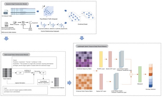
Figure 1.
Overview framework of DLG–IDS.
3.1. Dynamic Graph Construction Module
Industrial control systems typically include devices such as SCADA, PLCs, sensors, and actuators, with network traffic data packets representing the communication interactions between these devices, while the control component involves the logical or physical control processes between the devices. Moreover, considering the significant spatio–temporal dynamic characteristics of industrial control network traffic data, traditional static graph models struggle to capture the temporal evolution patterns of device interactions. To address this, the proposed framework introduces a dynamic graph construction method based on multi–source data streams, mapping multimodal industrial control traffic data into two types of subgraph structures: the pcap network traffic subgraph and the control relationship subgraph, which are then merged into a unified graph structure.
The pcap network traffic subgraph is constructed based on the temporal propagation paths of data packets, forming a chain–like topological structure. For the packet sequence within a time window , each packet contains the source device IP , destination device IP , protocol type , and timestamp , which can be mathematically represented as shown in Equation (1). The set of nodes represents device entities. The set of edges and directed edges indicate network communication from node to node . The time axis is divided into multiple continuous windows of equal time intervals, with each window corresponding to an instance of a dynamic graph , thereby constructing the time–series graph .
Within each time window , the communication count between device and device is calculated, and the edge weight is defined by incorporating a protocol importance weight function , as represented by Equation (2), and then construct the adjacency matrix for the time window .
where the communication count statistics and the protocol weight function are represented by Equation (3) and Equation (4), respectively.
As the time window slides, the adjacency matrix is dynamically updated to reflect real–time communication patterns. At the end of each window, the data from the old window are discarded, and new window data are loaded. The edge weights are recalculated according to Equation (5).
The protocol weight can also be dynamically updated based on network security policies, for example, by reducing the weight of a protocol that has been frequently attacked. Specifically, the protocol weight adjustment is given by
where is the decay factor and AttackFreq represents the historical attack frequency of the protocol.
The control relationship subgraph is used to model the logical control dependencies between devices in an industrial network. The set of nodes represents all devices in the control system, and the set of edges represents the control dependencies between devices. Specifically, if device controls device , an edge exists between them.
The node feature matrix is . Each node’s feature vector contains information such as the device type, role, and permission level.
Here, denotes the device type, where the master computer is assigned 0, the controller 1, the sensor 2, and the actuator 3; indicates the control role, with the controlling side set to 0 and the controlled side to 1; represents the control priority, with high assigned as 2, medium as 1, and low as 0.
The adjacency matrix of the control relation subgraph is defined as follows:
When the network topology changes due to the addition or removal of devices or adjustments in permissions, the adjacency matrix needs to be dynamically updated.
If a new device is managed by controller , the adjacency matrix is expanded accordingly.
If the device loses control over device , the corresponding entry in the adjacency matrix is changed to .
For complex hierarchical structures, we introduce a multi–hop adjacency matrix,
where represents a k–hop control path, and K is the maximum number of hops.
To comprehensively model the spatio–temporal dynamics and logical control hierarchy of industrial networks, it is necessary to organically combine the pcap network traffic subgraph with the control relationship subgraph.
By weighted fusion of the dynamic communication adjacency matrix and the static control adjacency matrix , a comprehensive adjacency matrix is generated as follows:
In Equation (11), represents the dynamic communication weight, reflecting the importance of real–time traffic patterns, while represents the static control weight, reflecting the priority of logical control dependencies. The constraint is .
3.2. Multi–Modal Feature Enhancement Module
At the node feature level, this study proposes a large language model (LLM)–driven semantic enhancement strategy to address the issue of insufficient feature representation in traditional methods, which often overlook the protocol semantic context. To handle the multimodal characteristics of industrial network traffic, including numerical statistical features and protocol text features, fine–grained feature fusion is achieved through the following steps:
- LLM Semantic Embedding GenerationTo enhance the semantic richness and interpretability of the initial node features, a two–stage feature enhancement strategy is designed by combining the reasoning capabilities of large language models (LLMs) with the efficient adaptability of lightweight language models.Raw protocol text and device logs from node features are input into the LLM, and prompt engineering is used to guide the LLM in generating two types of outputs: one is a prediction label, which infers whether the operation type is normal or anomalous based on the text content; the other is a natural language description, which outlines the operation intent and potential risks. An example of the input and output of the LLM is shown in Figure 2.
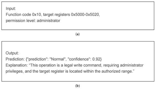 Figure 2. (a) The input to the LLM comes from feature information such as function codes and permission levels in the original text and logs. (b) The output of the LLM includes predicted labels and natural language explanations of the input features.The original text, prediction label, and explanation are merged to form enhanced text as Equations (12) and (13), and the lightweight language model (LM) is fine–tuned using the objective functions from Equation (14) to Equation (16).The mask tokens in the enhanced text are reconstructed to calculate the Masked Language Modeling (MLM) loss , and a prediction consistency loss is computed by constraining the LLM’s generated label to match the LM’s prediction. The total loss function is the weighted sum of the MLM loss and the prediction consistency loss.
 - Multi–modal Feature ConcatenationThe fine–tuned language model is then used to encode the original text, generating enhanced semantic embeddings.These enhanced semantic embeddings are fused with the original node features, including dynamic traffic features and static control attributes, to create a comprehensive feature representation as follows:This operation initially merges numerical statistical features with semantic context but does not explicitly model the relationships between the modalities.
- Cross–Modal Attention AlignmentTo eliminate the spatial heterogeneity of multimodal features, a dual–stream cross–attention mechanism is designed as follows:A query vector is extracted from the traffic features , focusing on real–time communication patterns. Keys and values are extracted from the semantic embeddings E, encoding protocol semantic information. The generation of Q, K, and V are shown in Equations (19), (20), and (21), respectively.The attention weights are computed using a scaled dot–product attention mechanism to measure the correlation between traffic features and semantic features, as shown in Equation (22). Then weighted aggregated semantic information to the traffic feature space, as in Equation (23).To prevent information loss and improve training stability, the fused features are added to the original concatenated features, followed by layer normalization,where is the projection matrix used to align the dimensions of the concatenated features and the fused features.
3.3. Lightweight Spatio–Temporal Graph Neural Network
To reduce computational complexity and adapt to the resource constraints of industrial edge devices, this paper designs a lightweight spatio–temporal graph neural network, incorporating sparse graph attention network (Sparse GAT) and local window Transformer to lower computational overhead. The joint adjacency matrix (N is the number of nodes) from Section 3.1 and the enhanced multimodal feature matrix (N is the number of nodes, T is the number of time steps, and d is the feature dimension) from Section 3.2 are input into the network for anomaly detection. The specific process is as follows:
- Time Feature Extraction ProcessBi–GRU extracts temporal features from each node in the graph structure across sequential time steps,where h denotes the hidden layer dimension of the GRU, with bidirectional outputs concatenated into a –dimensional vector. The temporal feature matrix is subsequently generated by the Bi–GRU.A Sparse GAT operates by exclusively computing attention weights between each node and its Top–K neighbors, formally expressed aswhere denotes the learnable weight matrix, is the attention vector, and represents the Top–K neighbor set of node .The spatial feature matrix is obtained through feature aggregation governed by Equation (28).Therefore, at each time step t, the spatial relationships between nodes are modeled through the following formulation:where denotes the output dimension of SparseGAT Layer. Compared to the original GAT, the computational complexity of SparseGAT is reduced from to .The integration of graph Transformer layers enhances the model’s capacity to capture long–range temporal dependencies and complex spatial interactions, while the local window attention mechanism restricts each node’s temporal attention scope to a fixed interval at step t, as formalized by Equations (30) and (32).where denote learnable parameter matrices, and w specifies the local window size. The windowed temporal attention outputs features with dimension through Equation (33). This design reduces the computational complexity of the Transformer layer from to .
- Spatial Feature Extraction ProcessThe spatial feature extraction branch directly models spatial dependencies through the combined adjacency matrix while employing local windowed attention along the spatial dimension as formalized in Equations (34) and (35). The network structure of its layers is designed in the same way as in the temporal feature extraction in the previous item.
- Graph–Level Feature Generation and Anomaly DetectionThis module generates anomaly probabilities for network traffic by globally aggregating and mapping multi–modal spatiotemporal features, thereby providing direct evidential support for security decision–making in industrial control systems.Extend the temporal features along the spatial dimension to and the spatial features along the temporal dimension to , ensuring dimensional consistency before concatenating them into .This design enables the model to adaptively adjust spatio–temporal weights based on the characteristics of the attack. For example, for slow infiltration attacks that depend on long–term temporal patterns, the model may assign higher weight to the temporal path, whereas for lateral movement attacks that rely on abnormal topological propagation, the spatial path weight is increased.
4. Evaluation
4.1. Experimental Settings
The experimental environment was configured to ensure the accurate assessment of the DLG–IDS framework. The hardware foundation consisted of an NVIDIA A800 80 GB PCI–e GPU and an Intel Xeon Gold 6430 CPU. This combination provided the necessary computational power to handle the complex operations involved in dynamic graph construction, multi–modal feature processing, and the functioning of the lightweight spatio–temporal graph neural network. On the software side, Python 3.7 served as the primary programming language, facilitating the implementation of the proposed algorithms. PyTorch 1.12.1 was utilized as the deep–learning framework, enabling efficient model training and inference. CUDA 11.6 was integrated to accelerate the GPU–based computations, significantly reducing the processing time. DGL 0.9.1 was employed for dynamic graph construction, allowing for the real–time representation of network traffic and control relationships. HuggingFace Transformers 4.25.1 was used for multi–modal feature processing, especially in the context of leveraging large language models for semantic enhancement.
In the multi–modal feature enhancement module, the large language model LLaMA3–8B was selected to generate predictions and explanations for graph node features. Its powerful natural language understanding capabilities were harnessed to infer operation types from raw protocol text and device logs. The LM, DeBERTa–v3–base, was then fine–tuned. During training, the large language model was frozen to preserve its pre–trained domain knowledge while reducing computational overhead. The fine–tuning learning rate was set to , to achieve an optimal balance between model convergence and generalization.
In the lightweight spatio–temporal graph neural network, the Sparse GAT’s hidden layer dimension is set to 128 and is equipped with a 4–head attention mechanism to capture multi–granularity feature interactions. For each node, only the top 10 edges with the highest communication intensity are retained as Top–K neighbors, ensuring both sparsity and efficient computation of the graph structure. The local window Transformer layer employs a window size of and is configured with an 8–head attention mechanism to extract local spatio–temporal dependencies. Model training is conducted using the Adam optimizer with a learning rate of , a fixed batch size of 64, and over a total of 100 epochs.
4.2. Datasets for Evaluation
We validate the effect of the proposed model on two datasets: the publicly available dataset SWaT and the self–collected dataset SBFF, respectively. Some general information about the two datasets is shown in Table 1 below.

Table 1.
General information of the datasets.
This study utilizes the SWaT dataset [25] developed by the Singapore University of Technology and Design, collected from a real–world water treatment testbed. The platform employs Ethernet/IP protocol communication and features a six–stage treatment process: Raw Water Tank (RWT), Pretreatment (coagulation and sedimentation), Ultrafiltration (UF), Dechlorination, Reverse Osmosis (RO), and UV Disinfection. The dataset includes time–series data from 51 sensors and actuators, capturing 11 consecutive days of operation—7 days under normal conditions followed by 4 days under cyber–attacks. It comprehensively documents water supply, filtration, backwashing, and other processes, offering a complete operational scenario for security research in water treatment systems.
The normal data of the SBFF dataset used in this study were collected by us in a real industrial production environment, and the malicious data were collected on the industrial control system simulation platform ICSSIM [26].
We established a simple simulated network architecture for a bottle–filling factory on this platform. As illustrated in Figure 3, the management and control layer comprises three HMIs, with the attacker generator also situated at this layer. Two independent PLCs manage distinct hardware zones: PLC–1 controls the water tank and valves, while PLC–2 oversees the conveyor belt. Network configurations for each ICS node are provided in Table 2, and communication is conducted using the Modbus protocol.
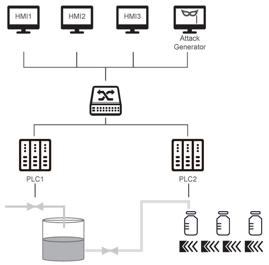
Figure 3.
Control network architecture for the bottle filling factory.

Table 2.
Node network configuration for the bottle filling factory.
We selected four typical attack types targeting ICS and obtained attack traffic on the simulation platform, and the specific numbers are shown in Table 3.

Table 3.
Number of different categories of flows in the dataset SBFF.
Reconnaissance Attack: This attack does not directly affect industrial production but involves an intruder gathering information by scanning MAC addresses, IP addresses, and open ports. The attack is carried out using Ettercap to broadcast ARP for IP scanning, along with Nmap for port scanning.
Replay Attack: In this scenario, the attacker maliciously retransmits packets captured during normal system operations to disrupt the control system’s proper functioning. The attack is implemented using the Scapy library in conjunction with ARP spoofing and MitM techniques to sniff network packets for 15 s, after which the captured packets are replayed three times (a total of 45 s).
DDoS Attack: Multiple attackers send a large volume of packets to the network or specific services, causing a denial of service in control system components. This attack leverages network addresses collected during reconnaissance and Modbus addresses sniffed from the network. Using the “DDoSAgent” class in ICSSIM, 800 instances are generated, with each instance sending read requests to a PLC continuously for 60 s, resulting in severe communication delays in the ICS network during the attack.
MitM Attack: In this attack, the adversary injects false data to intercept or manipulate communication between two ICS components. The attack is conducted by performing ARP poisoning on ICS components to redirect packets to the attack node. The attacker intercepts packets and modifies Modbus write requests and read responses to send manipulated packets to predetermined destinations, and ARP messages are sent to ICS components to clear routing tables.
4.3. Performance Metrics
To comprehensively evaluate the performance of the proposed DLG–IDS framework, we adopt the following metrics commonly used in machine learning and anomaly detection. These metrics assess the model’s detection accuracy, computational efficiency, robustness, and practical applicability in industrial control networks.
Precision was defined as Equation (41), where (True Positive) represented the number of malicious traffic instances correctly identified by the model, and (False Positive) was the number of benign traffic instances incorrectly classified as abnormal. Precision was crucial, as it measured the proportion of correctly identified anomalies among all predicted anomalies. A high Precision value minimized unnecessary operational interruptions caused by false alarms in industrial control networks.
Recall was calculated as Equation (42), where (false negative) was the number of malicious traffic instances erroneously labeled as benign. Recall indicated the fraction of true anomalies correctly detected by the model. Maximizing Recall was essential to ensure minimal missed detections of critical threats in industrial systems.
The F1–score, which balanced the trade–off between false positives and false negatives, was computed as Equation (43). In imbalanced datasets, where anomaly samples were rare, the F1–score provided a more comprehensive measure of the model’s performance.
The false positive rate () was given by Equation (44), where (True Negative) was the number of benign traffic instances accurately recognized as normal. A low was essential in industrial settings to avoid unnecessary downtime.
In addition to these metrics, the Area Under the Receiver Operating Characteristic (ROC) Curve (AUC–ROC) was used. The ROC curve plotted the against the at various classification thresholds. The AUC–ROC provided an overall measure of the model’s ability to distinguish between normal and abnormal traffic, with a higher value indicating better performance. The Precision–Recall (PR) curve was also employed, particularly important for imbalanced datasets where anomalies are rare. It plots Precision against Recall across different thresholds, with the area under the PR curve (AUC–PR) providing a comprehensive view of the trade–off between detection accuracy and coverage. The FPR at a specific TPR (e.g., 95% TPR) was reported to assess the false alarm rate under high–detection scenarios, critical for operational environments where missed threats are unacceptable. Detection Error Tradeoff (DET) curves, which plot miss rate (FNR) against FPR on normal deviate scales, were used to visualize the error trade–offs more sensitively than ROC curves, especially in the low–FPR region. Finally, calibration plots (reliability diagrams) were generated to evaluate how well the predicted probabilities align with the actual likelihood of being an anomaly, essential for trustworthiness in security decision–making. This study utilized the aforementioned curves to comprehensively evaluate the performance of detection models.
Detection latency, measured in milliseconds, was the time required to process a single network traffic time window. This metric was of utmost importance in real–time industrial control systems, where timely detection of anomalies was crucial to prevent potential damages.
4.4. Ablation Experiment
Ablation experiments were systematically conducted to evaluate the contributions of each core component of the DLG–IDS framework. We use an unoptimized spatio–temporal graph neural network as the base model for detection, and the results of the ablation experiments on the SWaT and SBFF datasets are shown in Table 4 and Table 5, respectively. The experimental results on SWaT show that the base model, without any additional enhancements, achieved an F1–score of 0.770, a FPR of 0.220, and a detection latency of 189 ms. The pure time–series architecture LSTM was used as a baseline for the ablation experiments. The base model alone achieves an F1–score of 0.770, which is substantially higher than the 0.604 F1–score of the traditional LSTM baseline. This confirms the fundamental advantage of the proposed architecture over conventional sequential models. After incorporating the LM structure into the base model, the F1–score showed a marked improvement. When the LLM–LM semantic enhancement module was integrated, the F1–score improved to 0.852, and the FPR decreased significantly to 0.06. However, the latency increased to 212 ms. The results of the SBFF dataset also show the same trend. This increase in latency was due to the additional computational requirements of the semantic feature extraction process. The LLM–LM module, by leveraging the reasoning capabilities of large language models and the fine–tuning of lightweight language models, enhanced the model’s ability to understand protocol semantics. This, in turn, led to a more accurate detection of anomalies, as it could identify subtle semantic differences that the base model might have missed.

Table 4.
Ablation experiments on the SWaT dataset.

Table 5.
Ablation experiments on the SBFF dataset.
The introduction of the Sparse GAT demonstrated significant advantages. The F1–score slightly increased to 0.796 and 0.656, respectively, while the latency decreased by approximately 50% compared to the base model. The sparse GAT is designed to calculate the attention weights only between each node and its Top–K neighbors. This method reduces the computational complexity, and by effectively capturing the abnormal propagation between devices, the sparse GAT improves the model’s performance in detection.
The local window Transformer further enhanced the model’s performance. The local window Transformer limits the temporal attention range of each node to a fixed interval. This localized attention mechanism was effective in modeling the periodic industrial operational patterns, as it focused on the relevant temporal and spatial dependencies within the local window.
When all the components—LLM–LM, Sparse GAT, and local window Transformer—were combined with the base model, the system achieved optimal performance. On the SWaT dataset, the F1–score reached 0.943, representing a 22.4% improvement over the base model. The FPR dropped to 0.046, a 79.1% reduction, and the latency was controlled at 71 ms, a 62.4% acceleration. On the SBFF dataset, the optimization degrees of these three performance indicators are 41.3%, 82.4%, and 53.2%, respectively.
These results not only validated the effectiveness of the multi–modal fusion strategy but also demonstrated the model’s adaptable configurability and its balanced design between computational efficiency and detection reliability. Specifically, the semantic features from the LLM–LM module strengthened the understanding of protocol context, the sparse graph structures of the Sparse GAT optimized the modeling of spatial dependencies, and the localized temporal attention of the local window Transformer precisely tracked the evolution of device states—collectively contributing to the observed performance improvements.
4.5. Comparative Experiment
To validate the superiority of the proposed DLG–IDS framework, comparative experiments were conducted against three representative baseline methods: Random Forest (RF), Graph Convolutional Network (GCN), and OFA [27] (a state–of–the–art industrial anomaly detection model in recent years). The performance comparison was carried out on both SWaT and SBFF datasets, with detailed metrics shown as Table 6 and Table 7.

Table 6.
Performance comparison of four methods on the SWaT dataset.

Table 7.
Performance comparison of four methods on the SBFF dataset.
DLG–IDS has demonstrated excellent performance in overall accuracy across different datasets, achieving 0.975 and 0.986 on the two industrial traffic datasets, respectively. This indicates that DLG–IDS is highly effective in classifying traffic instances both in simulated and real industrial control scenarios. In terms of Precision, DLG–IDS outperformed the other methods. The higher Precision of DLG–IDS indicated its ability to accurately identify anomalies without generating excessive false alarms. Regarding Recall, DLG–IDS also demonstrated superiority. The higher Recall of DLG–IDS suggested its improved ability to detect stealthy attacks, such as parameter tampering within compliant protocols. This was in line with its design principles, where the dynamic graph construction captured real–time communication patterns, and the LLM–driven semantic enhancement deciphered protocol intent. The F1–score, which balanced Precision and Recall, also showed DLG–IDS’s advantage. DLG–IDS’s optimal F1–scores indicated robust detection accuracy with minimal false positives and false negatives.
The ROC curve and its AUC value are fundamental tools in evaluating the performance of binary classification models, especially relevant in anomaly detection tasks like industrial network security. Figure 4 shows the ROC curves and AUC values of the four models tested on the two given datasets.
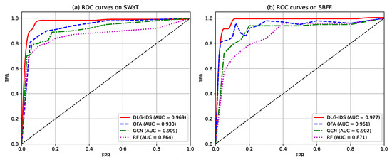
Figure 4.
ROC curves of the four intrusion detection methods.
Across both datasets, DLG–IDS’s AUC values (0.969 on SWaT; 0.977 on SBFF) not only lead but also exhibit minimal variance, showcasing strong cross–dataset adaptability. This stability stems from its ability to capture both protocol–level semantics and spatio–temporal dependencies in network traffic, essential for ICS with dynamic operation modes. In contrast, the other three models show consistent performance ranking (OFA > GCN > RF) but larger AUC fluctuations, indicating weaker generalization. Such results validate Model DLG–IDS as a robust candidate for securing ICS, while the others may require context–specific tuning or remain supplementary in resource–constrained deployments. ROC–AUC analysis corroborates that model DLG–IDS outperforms competitors in distinguishing normal and anomalous behavior across industrial datasets. Its superior discriminative power, coupled with cross–dataset stability, positions it as a pragmatic solution for real–world ICS security, where minimizing false alarms and maximizing threat detection are paramount.
Building upon the ROC curves that have demonstrated the overall classification performance of various intrusion detection methods, the following Figure 5 further focuses on specific to compare the of each method on the SWaT and SBFF datasets. From Figure 5a, it can be observed that the of DLG–IDS, OFA, and GCN are all close to 1.0 at each level, whereas the of RF is relatively slightly lower. From Figure 5b, the of DLG–IDS and OFA are still close to 1.0 at different ; when , the of GCN is slightly lower than that of the former two methods, and the of RF becomes more similar to that of other methods at high . The variation trend of for different methods with the increase in is relatively stable, and the differences in performance between the two datasets are to some extent consistent. This underscores DLG–IDS’s superiority in sustaining both high detection rates and low false alarm rates across different datasets and TPR demands.
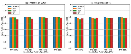
Figure 5.
Comparison of FPR at specific TPRs for different intrusion detection methods.
PR (Precision–Recall) curves are critical for assessing intrusion detection performance, as they reflect the trade–off between Precision, which is about avoiding false positives, and Recall, which is about detecting true positives. Figure 6 displays PR curves of four methods on the SWaT and SBFF datasets, with Average Precision (AP, the area under the PR Curve, similar to the AUC value in the ROC Curve) labeled for each method. For both datasets, DLG–IDS exhibits outstanding performance: On SWaT, its PR curve maintains a higher Precision across most Recall ranges, with the highest AP. On SBFF, DLG–IDS’s PR curve also leads, sustaining stronger Precision as Recall increases, and it achieves the highest AP as well. In comparison, other methods show lower Precision at similar Recall levels or lower AP scores. This demonstrates that DLG–IDS excels at detecting intrusions while keeping false alarms to a minimum, outperforming OFA, GCN, and RF on both datasets.
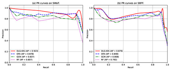
Figure 6.
PR curves of the four intrusion detection methods.
DET (Detection Error Tradeoff) curves are plotted to provide a comprehensive view of a classification model’s performance by illustrating the trade–off between two types of errors–false alarms and missed detections—across various decision thresholds. This is particularly critical in security applications like intrusion detection, where the cost of a false acceptance (, allowing an attack) is balanced against the cost of a false rejection (, flagging normal behavior as an attack). Unlike ROC curves, DET curves use a non–linear scale that magnifies differences in the critical low–error rate region, making them ideal for comparing performance in high–stakes environments.
As illustrated in Figure 7, the DET curves for the four methods on both the SWaT and SBFF datasets reveal clear performance distinctions. The DIG–IDS method consistently demonstrates superior performance, with its curve positioned closest to the origin of the graph on both datasets. This indicates that DIG–IDS achieves the most favorable balance between and , meaning it can effectively minimize both missed attacks and false alarms simultaneously across a wide range of operational thresholds. The other three methods exhibit varying levels of performance. The OFA and GCN models show intermediate results, with OFA performing well at very low false alarm rates, but its error rates increasing more rapidly than DIG–IDS as the threshold is adjusted. GCN presents a more stable but overall less optimal trade–off. In contrast, the RF method, a traditional machine learning approach, is significantly outperformed by the deep learning–based models on both datasets. Its curve is positioned highest, indicating consistently higher error rates for both and . This performance gap underscores the limitation of conventional methods in capturing the complex temporal and structural patterns in modern industrial control system data.
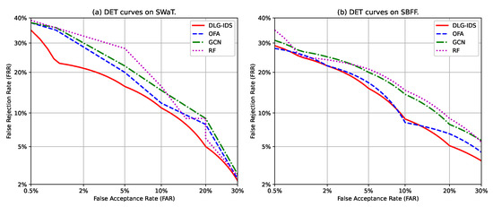
Figure 7.
DET curves of the four intrusion detection methods.
Calibration plots, or reliability curves, are essential for evaluating not only the accuracy but also the trustworthiness of a probabilistic classifier’s predictions. A model is considered well–calibrated when its confidence scores accurately reflect the true likelihood of an event. For security applications, this is critical because operational decisions rely on the credibility of these scores. A model that is accurate but poorly calibrated may mislead analysts by being systematically overconfident or underconfident.
The reliability curves and Expected Calibration Error (ECE) scores in Figure 8 clearly differentiate the calibration quality of the four methods. DIG–IDS demonstrates the best calibration performance on both datasets, with the lowest ECE values of 0.031 on SWaT and 0.036 on SBFF. Its curve closely aligns with the ideal diagonal, indicating that its confidence measures are highly reliable. OFA also shows strong calibration, particularly on the SWaT dataset, where it nearly matches the performance of DIG–IDS. In contrast, the GCN model shows noticeable miscalibration, while the RF method performs the poorest with significantly higher ECE scores. The RF curve deviates substantially from the ideal line, reflecting a tendency toward overconfident predictions. This is a common trait in ensemble methods like random forests, which often require post–processing to produce well–calibrated probability estimates. These results highlight that strong detection capability must be accompanied by reliable confidence scoring for practical deployment. A model like GCN may detect anomalies effectively but remains less useful if its confidence scores cannot be trusted. DIG–IDS excels not only in detection accuracy but also in providing well–calibrated confidence estimates, making it particularly suitable for real–world security operations.
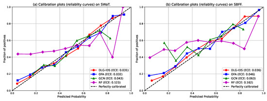
Figure 8.
Reliablity curves of the four intrusion detection methods.
To further dissect the classification performance of the four methods, confusion matrices were employed. These matrices offer a granular view of TP, TN, FP, and FN, enabling precise quantification of misclassification patterns across the SWaT and SBFF datasets, as shown in Figure 9 and Figure 10. Across both datasets, clear performance gradients emerge. On the SWaT dataset, RF shows symmetric misclassification tendencies, with non–negligible errors in both false alarm (FP) and missed threat (FN) rates. GCN improves threat detection (lower FN) but still struggles with false alarms (higher FP). OFA advances toward more reliable classification, yet DLG–IDS stands out, minimizing both FP and FN through its adaptive design. On the SBFF dataset, the trend persists. RF and GCN retain residual misclassification issues—RF with notable false alarms, GCN with lingering missed threats. OFA approaches high reliability but falls short of DLG–IDS. The latter delivers near–perfect results, showcasing its superiority in handling complex attack scenarios.

Figure 9.
Confusion matrices of the four intrusion detection methods on the SWaT.

Figure 10.
Confusion matrices of the four intrusion detection methods on the SBFF.
5. Security Analysis
5.1. Different Attack Scenario Simulation Experiment
To better evaluate the adaptability of the models in different network attack scenarios, we conducted comparative tests on the performance of each model under the scenarios of normal production environment traffic and four types of attack traffic in the SBFF dataset, with the results shown in Figure 11.
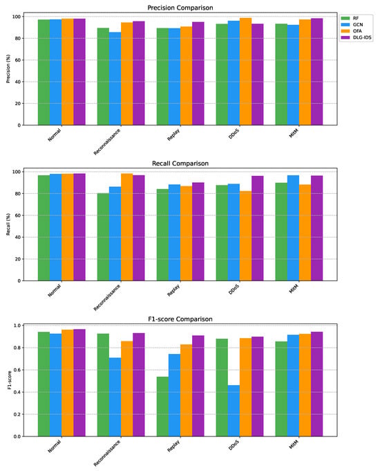
Figure 11.
Performance comparison experiments under different attack scenarios.
In the normal scenario, several methods achieve high Precision with small differences, indicating that different algorithms can all achieve relatively good classification results when dealing with normal network traffic. In attack scenarios, however, the performance of some methods fluctuates significantly. For example, the F1–score of GCN in the DDoS attack scenario is only 0.48, and it also achieves the lowest F1–score of 0.71 in the reconnaissance attack scenario, which indicates that GCN is not good at detecting these two types of attacks. Similarly, RF performs poorly in detecting replay attacks, but both of the methods can achieve an F1–score of over 0.8 in detecting MitM attacks.
By contrast, the other two detection methods, OFA and DLG–IDS, perform more stably across various attack scenarios. OFA achieves a slightly higher Precision in DDoS detection, possibly due to its “stricter feature extraction of attack traffic”. However, this comes at the cost of partial Recall, which may lead to missed detections. Overall, DLG–IDS achieves higher F1–scores, all exceeding 0.9, indicating that it has a better balance between accurate identification and comprehensive capture of attacks. In contrast, OFA may be slightly inferior in the coordination between Precision and Recall.
This result showed that the model could handle complex, multi–faceted attack scenarios that were more representative of real–world cyber threats in industrial control systems.
5.2. Scalability Experiment
As industrial control networks are constantly evolving and expanding, the scalability of the anomaly detection framework is of great significance. A scalability experiment was designed to test the framework’s performance as the network size increased.
The SBFF dataset was extended to simulate a larger–scale industrial network. In the original SBFF dataset, there are only 6 nodes. We expanded the node number to 12, 18, and 24, and the number of collected network flows was doubled accordingly, resulting in three extended datasets. The experimental results on these datasets are shown in Table 8.

Table 8.
Performance comparison of different methods on extended dataset.
The results showed that as the network size grew, DLG–IDS showed almost no degradation in detection performance, with the detection latency increasing slightly from 51 ms to 56 ms. The DLG–IDS method significantly outperforms all other methods across all three datasets and all evaluation metrics. Its accuracy consistently exceeds 0.976, and its F1–score remains above 0.906, demonstrating exceptional robustness and effectiveness in intrusion detection regardless of network scale. Unlike DLG–IDS, which shows minimal fluctuation in metrics, other methods, especially RF and OFA, exhibit more significant performance degradation as the number of nodes increases. Although GCN performs worse than OFA in terms of detection performance, its metrics remain relatively stable in the experiments on extended datasets. OFA achieves good accuracy and Recall especially in smaller networks, but suffers from lower Precision, indicating a higher rate of false positives. This trade–off results in a lower F1–score than GCN in most cases. This, to some extent, verifies the role of graph neural networks in capturing changes in network structures.
In addition to the magnitude of metric fluctuations, there is also a significant performance gap in absolute values between DLG–IDS and other methods. For example, in the 12–node network, DLG–IDS’s F1–score is 12.8% higher than the next best. Its accuracy is at least 5.4% higher than alternatives. DLG–IDS achieves the best balance between Precision and Recall. Its Precision and Recall values are consistently high and closely aligned. In contrast, other methods exhibit larger disparities, indicating DLG–IDS minimizes both false positives and false negatives more effectively. This underscores DLG–IDS’s significant advancement over traditional ML (RF), graph–based learning (GCN), and other advanced techniques (OFA).
5.3. Case Study Analysis
In this section, we use the MitM and DDoS attacks from the SBFF dataset as case studies to demonstrate the specific operational workflow of DLG–IDS for intrusion detection.
Figure 12a and Figure 12b, respectively, show the original traffic pcap and log files of the MitM attack. In the pcap slice, the host first completes the resolution of IP and MAC addresses via ARP, and then uses Modbus TCP default port 502 to transmit data, which reflects the network communication characteristics in industrial scenarios. However, it is difficult to distinguish between normal communication and attack traffic based solely on the preliminary analysis of traffic files. The log file records the step–by–step operations of the communication process in a structured and semantic format, showing obvious signs of ARP spoofing. The attacker (192.168.0.41) manipulates ARP responses to associate its own MAC address with the IP addresses of critical assets such as PLC1 (192.168.0.11) and HMI1 (192.168.0.21), which enables the attacker to intercept and tamper with subsequent TCP and Modbus communications. For example, entries such as “ARP PLC1/192.168.0.11/arp–cache” and “Modbus PLC1/192.168.0.11/reg–0x0001” reflect the execution of malicious operations, including register tampering and abnormal value injection. The log also indicates that a threshold alert is triggered when the register value exceeds the expected range.
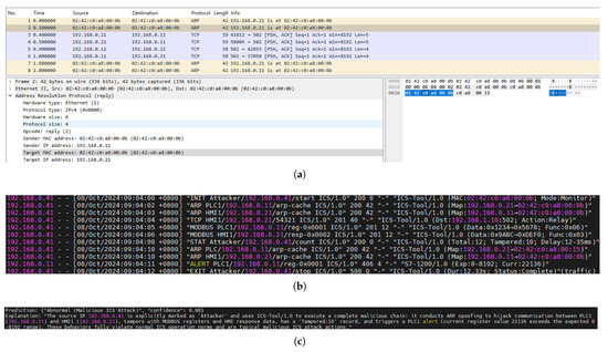
Figure 12.
(a) Pcap slice of the MitM attack. (b) Log slice of the MitM attack. (c) LLM–generated prediction and explanation for the MitM attack.
Most notably, Figure 12c demonstrates the ability of LLM to automatically synthesize information from high–level logs and generate coherent, accurate natural language explanations. Predictions indicate that this network flow is abnormal traffic with a confidence level of 0.98. The explanation further states that the attacker hijacked the communication between the PLC and HMI in the industrial control system through ARP spoofing, and used ICS–Tool/1.0 to tamper with Modbus registers and HMI response data—causing the PLC register values to exceed the normal range and trigger an alert. Beyond identifying the attack type and source, LLM can also correlate technical evidence across different levels. This demonstrates the potential role of LLM as an explanation layer in intrusion detection systems, converting multimodal security data into actionable insights for analysts.
Similarly, Figure 13 shows another type of attack, DDoS, including its traffic slice log slice, as well as the predictions and explanations generated by LLM. The pcap file shows that multiple source hosts are continuously sending requests to Modbus default port 502 of the target host (192.168.0.11), with the function code being 3 (Read Holding Registers). While the LLM predicts with a high confidence level of 0.99 that this is a DDoS attack targeting the ICS. The explanation indicates that IP addresses from multiple network segments are marked as attackers, which launched 220 requests within 60 s via “DDoSAgent/1.0” (attack mode). Firstly, an “Excessive Requests” alert was triggered due to the request rate (1200 requests per second), and then a “Service Unavailable” alert was triggered due to the response delay (4500 ms), completely disrupting the normal operation of the PLC. These behaviors—including distributed collaborative requests via DDoS tools, explicit attacker labeling, and PLC service failures—violate ICS operation norms and align with the typical characteristics of DDoS attacks.
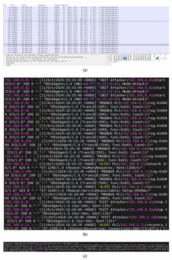
Figure 13.
(a) Pcap slice of the DDoS attack. (b) Log slice of the DDoS attack. (c) LLM–generated prediction and explanation for the DDoS attack.
Together, these results highlight the value of integrating heterogeneous data sources—network traffic, system logs, and semantic interpretatio—for robust and explainable attack diagnosis. Such an approach can significantly enhance detection transparency and reduce response time in operational ICS environments.
Figure 14 shows the graph construction visualization results of two types of attack traffic in the proposed DLG–IDS framework. Figure 14a corresponds to the DDoS attack, presenting a topology where multiple source nodes centrally initiate connections to a single target nod—this reflects the core characteristic of DDoS attacks, in which multiple attack sources collaboratively send massive requests to the target to deplete its resources. Figure 14b corresponds to the MitM attack, presenting a topology where a single intermediate node intervenes in the communication links between multiple nodes—this reflects the typical pattern of MitM attacks, in which the attacker disguises itself as an intermediate hub to intercept or tamper with data between the two communicating parties. The graph structure clearly demonstrates the characteristics of different attack modes. In actual operation and maintenance processes, attacker nodes are marked in red in the graph structure, and the edges used to transmit attack communications are also assigned higher weights and different colors to distinguish them from normal communications. These visualizations help operation and maintenance personnel locate attacks faster and more accurately.
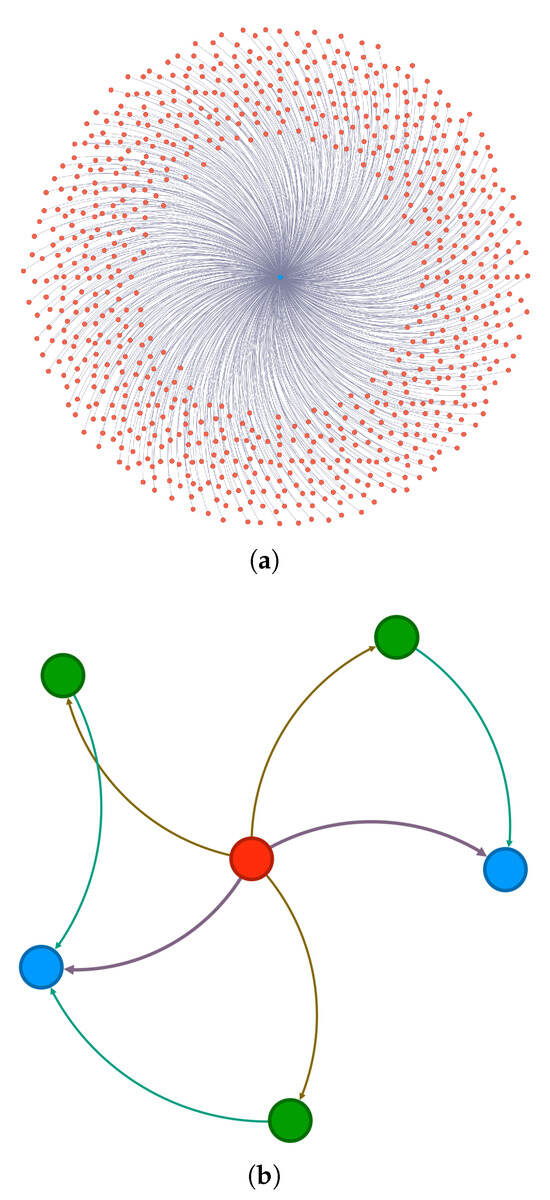
Figure 14.
(a) The graph structure of DDoS attacks. (b) The graph structure of MitM attacks. Red nodes represent attacker nodes, blue nodes represent compromised nodes, green nodes represent intermediate nodes, and edge thickness corresponds to the attack frequency.
In addition, Figure 15 also presents the anomaly score traffic time graphs for the two types of attacks, whose function is to conduct real–time monitoring of anomalies in industrial network traffic and quantify the level of attack threats through anomaly scores and the number of Modbus requests. The blue line quantifies the anomaly score reflecting the deviation of traffic from the normal state, the light blue bars represent the number of Modbus requests, and the red dashed line denotes the anomaly threshold (1.0). When an attack event causes anomalies in the volume of Modbus requests, the anomaly score will exceed the threshold, and alerts will be marked with red dots. Clicking on the data points of the line in the graph displays the specific information of the event; this information is associated with the predictions and explanations generated by LLMs. This helps security personnel quickly identify attacks, analyze the damage logic of attacks on industrial control devices, and support timely security responses and fault handling.
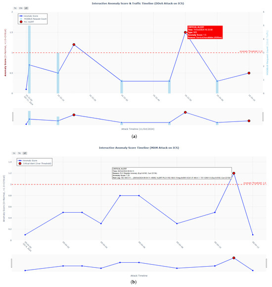
Figure 15.
(a) The anomaly score time graph of DDoS attacks. (b) The anomaly score time graph of MitM attacks.
6. Conclusions and Further Work
This work presents DLG–IDS, a novel intrusion detection framework that synergizes dynamic graph modeling, LLM–based semantic enhancement, and lightweight STGNN design to overcome the fragmentation in traditional ICS security approaches. By constructing a unified dynamic graph that integrates real–time communication patterns with control dependencies, the framework effectively captures spatiotemporal dynamics while leveraging LLMs to generate contextual semantic embeddings aligned with traffic attributes through cross–modal attention—significantly enhancing detection of covert attacks such as parameter tampering within compliant protocols. Furthermore, the introduction of sparse graph attention and local window Transformers reduce computational complexity from quadratic to linear without compromising accuracy, addressing the critical conflict between resource constraints and real–time requirements in industrial edge devices. Rigorous evaluations confirm these advancements: DLG–IDS achieves a 41.3% higher F1–score and 82.4% lower false positives versus base models on the SBFF dataset, alongside a 53.2% reduction in latency, while scalability experiments demonstrate consistent performance as network size expands. These results collectively position DLG–IDS as a pragmatic, high–performance solution for modern ICS environments.
However, we acknowledge that the integration of large–scale LLMs introduces non–negligible computational overhead, which may challenge deployment in resource–limited ICS edge devices. To mitigate this, future work will explore model compression techniques such as pruning and knowledge distillation to reduce LLM size while preserving semantic reasoning capabilities. Additionally, the edge–cloud collaborative inference strategy is also a feasible approach, where lightweight models run locally on edge devices for real–time detection, while complex semantic parsing is offloaded to cloud–based LLMs only when necessary. Such a hybrid approach could balance latency and accuracy more effectively in mission–critical ICS operations.
It should be noted that, given the existence of mature locally deployed large language model platforms, in the current implementation, the LLM semantic enhancement module operates by calling the platform’s basic APIs rather than redeploying complete large models. This choice reduces a portion of the workload but also introduces reliance on network connectivity and potential API latency. Regarding the trade–off between semantic richness and latency observed in ablation studies, we have also noticed that while LLM–enhanced features improve detection accuracy, they do introduce additional processing time. In real–world industrial control system setups, millisecond–level responsiveness is crucial, and this trade–off must be carefully managed. Future work will include more detailed analysis of latency thresholds for different industrial scenarios, such as safety–critical systems and monitoring–only systems, and exploration of adaptive semantic enhancement—enabling LLM features only for high–risk or ambiguous traffic patterns to minimize average latency without compromising security.
While DLG–IDS exhibits strong performance in evaluated scenarios, its reliance on LLMs for semantic parsing necessitates domain–specific fine–tuning to handle proprietary or non–standard industrial protocols, which currently limits broader applicability. Additionally, validation has primarily focused on water treatment systems, warranting further investigation into generalizability across diverse industrial domains such as power grids or manufacturing. Future efforts will explore adaptive LLM prompting strategies to mitigate protocol heterogeneity and investigate federated learning paradigms for privacy–preserving cross–organizational deployment. Further optimization via hardware–aware model compression techniques, such as quantization for ultra–low–resource edge devices, also represents a promising direction to enhance real–time responsiveness.
Author Contributions
J.L. designed and developed the model and wrote the original draft; J.W. conceived the experimental ideas and reviewed the original draft; T.Y., F.Q. and G.C. helped with data analysis and constructive discussions. All authors have read and agreed to the published version of the manuscript.
Funding
This study was partially supported by the National Key Research and Development Program of China: No. 2023YFC2605703 and No. 2023YFC2206402; the Cybersecurity Joint Defense System for Large Scientific Facilities Construction Project of the Chinese Academy of Sciences; and the Innovative Project of the Institute of High Energy Physics of the Chinese Academy of Sciences (No. E55456U210).
Institutional Review Board Statement
Not applicable.
Informed Consent Statement
Not applicable.
Data Availability Statement
The public dataset used to support the findings of this study can be found at: https://itrust.sutd.edu.sg/itrust-labs_datasets/dataset_info/ (accessed on 1 October 2025).
Conflicts of Interest
The authors declare no conflicts of interest.
References
- Ioulianou, P.; Vasilakis, V.; Moscholios, I.; Logothetis, M. A Signature–Based Intrusion Detection System for the Internet of Things. Inf. Commun. Technol. Form 2018. Available online: https://eprints.whiterose.ac.uk/id/eprint/133312/ (accessed on 2 October 2025).
- Moustafa, N.; Turnbull, B.; Choo, K.K.R. An ensemble intrusion detection technique based on proposed statistical flow features for protecting network traffic of internet of things. IEEE Internet Things J. 2018, 6, 4815–4830. [Google Scholar] [CrossRef]
- Bilot, T.; El Madhoun, N.; Al Agha, K.; Zouaoui, A. Graph neural networks for intrusion detection: A survey. IEEE Access 2023, 11, 49114–49139. [Google Scholar] [CrossRef]
- Altaf, T.; Wang, X.; Ni, W.; Yu, G.; Liu, R.P.; Braun, R. GNN–based network traffic analysis for the detection of sequential attacks in IoT. Electronics 2024, 13, 2274. [Google Scholar] [CrossRef]
- Hou, J.; Xia, H.; Lu, H.; Nayak, A. A graph neural network approach for caching performance optimization in ndn networks. IEEE Access 2022, 10, 112657–112668. [Google Scholar] [CrossRef]
- Wang, Y.; Li, J.; Zhao, W.; Han, Z.; Zhao, H.; Wang, L.; He, X. N–STGAT: Spatio–temporal graph neural network based network intrusion detection for near–earth remote sensing. Remote Sens. 2023, 15, 3611. [Google Scholar] [CrossRef]
- Gong, H.; Yan, C.; Xue, Y.; Guo, Y. Network Protocol Security Evaluation via LLM–Enhanced Fuzzing in Extended ProFuzzBench. In Proceedings of the International Conference on Intelligent Computing, Ningbo, China, 26–29 July 2025; Springer: Singapore, 2025; pp. 522–533. [Google Scholar]
- Cheung, S.; Dutertre, B.; Fong, M.; Lindqvist, U.; Skinner, K.; Valdes, A. Using model–based intrusion detection for SCADA networks. In Proceedings of the SCADA Security Scientific Symposium, Miami Beach, FL, USA, 24–25 January 2007; SRI International: Menlo Park, CA, USA, 2007; Volume 46, pp. 1–12. [Google Scholar]
- Hadžiosmanović, D.; Sommer, R.; Zambon, E.; Hartel, P.H. Through the eye of the PLC: Semantic security monitoring for industrial processes. In Proceedings of the 30th Annual Computer Security Applications Conference, Orleans, LA, USA, 8–12 December 2014; pp. 126–135. [Google Scholar]
- Yingxu, L.; Jiao, J.; Jing, L. Analysis of industrial control systems traffic based on time series. In Proceedings of the 2015 IEEE Twelfth International Symposium on Autonomous Decentralized Systems, Taichung, Taiwan, 25–27 March 2015; pp. 123–129. [Google Scholar]
- Ujjan, R.M.A.; Pervez, Z.; Dahal, K.; Khan, W.A.; Khattak, A.M.; Hayat, B. Entropy based features distribution for anti–DDoS model in SDN. Sustainability 2021, 13, 1522. [Google Scholar] [CrossRef]
- Wang, J. Industrial Internet of Things ARP Virus Attack Detection Method Based on Improved CNN BiLSTM. J. Cyber Secur. Mobil. 2024, 13, 1173–1206. [Google Scholar] [CrossRef]
- Dakheel, A.H.; Dakheel, A.H.; Abbas, H.H. Intrusion detection system in gas–pipeline industry using machine learning. Period. Eng. Nat. Sci. 2019, 7, 1030–1040. [Google Scholar] [CrossRef]
- Ridi, A.; Gisler, C.; Hennebert, J. Appliance and state recognition using Hidden Markov Models. In Proceedings of the 2014 International Conference on Data Science and Advanced Analytics (DSAA), Shanghai, China, 30 October–1 November 2014; pp. 270–276. [Google Scholar]
- Zhang, Y.; Yang, C.; Huang, K.; Li, Y. Intrusion detection of industrial internet–of–things based on reconstructed graph neural networks. IEEE Trans. Netw. Sci. Eng. 2022, 10, 2894–2905. [Google Scholar] [CrossRef]
- Athmane, M.M.B.; Soaïd, M.F.K.; Hamida, M.S.; Mohamed, M.M.; Karima, M.A. Building a Novel Graph Neural Networks–Based Model for Efficient Detection of Advanced Persistent Threats. 2023. Available online: https://www.researchgate.net/profile/Kamel-Ferrahi/publication/384225639_Building_a_novel_Graph_Neural_Networks-based_model_for_efficient_detection_of_Advanced_Persistent_Threats/links/67ab35108311ce680c5d44e7/Building-a-novel-Graph-Neural-Networks-based-model-for-efficient-detection-of-Advanced-Persistent-Threats.pdf (accessed on 2 October 2025).
- Cao, Y.; Jiang, H.; Deng, Y.; Wu, J.; Zhou, P.; Luo, W. Detecting and mitigating DDoS attacks in SDN using spatial–temporal graph convolutional network. IEEE Trans. Dependable Secur. Comput. 2021, 19, 3855–3872. [Google Scholar] [CrossRef]
- Wu, Y.; Dai, H.N.; Tang, H. Graph neural networks for anomaly detection in industrial Internet of Things. IEEE Internet Things J. 2021, 9, 9214–9231. [Google Scholar] [CrossRef]
- Ruan, W.; Chen, W.; Dang, X.; Zhou, J.; Li, W.; Liu, X.; Liang, Y. Low–rank adaptation for spatio–temporal forecasting. arXiv 2024, arXiv:2404.07919. [Google Scholar]
- Seyyar, Y.E.; Yavuz, A.G.; Ünver, H.M. An attack detection framework based on BERT and deep learning. IEEE Access 2022, 10, 68633–68644. [Google Scholar] [CrossRef]
- Abshari, D.; Fu, C.; Sridhar, M. LLM–assisted Physical Invariant Extraction for Cyber–Physical Systems Anomaly Detection. arXiv 2024, arXiv:2411.10918. [Google Scholar]
- Branescu, I.; Grigorescu, O.; Dascalu, M. Automated mapping of common vulnerabilities and exposures to mitre att&ck tactics. Information 2024, 15, 214. [Google Scholar] [CrossRef]
- Jonkhout, B. Evaluating Large Language Models for Automated Cyber Security Analysis Processes. Bachelor’s Thesis, University of Twente, Enschede, The Netherlands, 2024. [Google Scholar]
- Kotenko, I.; Abramenko, G. Detecting and Analysing Cyber Attacks Based on Graph Neural Networks, Ontologies and Large Language Models. In Proceedings of the 2025 IEEE 26th International Conference of Young Professionals in Electron Devices and Materials (EDM), Altai, Russian Federation, 27 June–1 July 2025; pp. 1460–1464. [Google Scholar]
- Mathur, A.P.; Tippenhauer, N.O. SWaT: A water treatment testbed for research and training on ICS security. In Proceedings of the 2016 International Workshop on Cyber–Physical Systems for Smart Water Networks (CySWater), Vienna, Austria, 11 April 2016; pp. 31–36. [Google Scholar]
- Dehlaghi–Ghadim, A.; Balador, A.; Moghadam, M.H.; Hansson, H.; Conti, M. ICSSIM—A framework for building industrial control systems security testbeds. Comput. Ind. 2023, 148, 103906. [Google Scholar] [CrossRef]
- Liu, H.; Feng, J.; Kong, L.; Liang, N.; Tao, D.; Chen, Y.; Zhang, M. One for all: Towards training one graph model for all classification tasks. arXiv 2023, arXiv:2310.00149. [Google Scholar] [CrossRef]
Disclaimer/Publisher’s Note: The statements, opinions and data contained in all publications are solely those of the individual author(s) and contributor(s) and not of MDPI and/or the editor(s). MDPI and/or the editor(s) disclaim responsibility for any injury to people or property resulting from any ideas, methods, instructions or products referred to in the content. |
© 2025 by the authors. Licensee MDPI, Basel, Switzerland. This article is an open access article distributed under the terms and conditions of the Creative Commons Attribution (CC BY) license (https://creativecommons.org/licenses/by/4.0/).