Abstract
The electrification of automotive powertrains has accelerated research efforts in the modeling, control, and monitoring of electric drive systems, where reliability, safety, and efficiency are key enablers for mass adoption. Despite a large corpus of literature addressing individual aspects of electric drives, current surveys remain fragmented, typically focusing on either multiphysics modeling of machines and converters, or advanced control algorithms, or diagnostic and prognostic frameworks. This review provides a comprehensive perspective that systematically integrates these domains, establishing direct connections between high-fidelity models, control design, and monitoring architectures. Starting from the fundamental components of the automotive power drive system, the paper reviews state-of-the-art strategies for synchronous motor modeling, inverter and DC/DC converter design, and advanced control schemes, before presenting monitoring techniques that span model-based residual generation, AI-driven fault classification, and hybrid approaches. Particular emphasis is given to the interplay between functional safety (ISO 26262), computational feasibility on embedded platforms, and the need for explainable and certifiable monitoring frameworks. By aligning modeling, control, and monitoring perspectives within a unified narrative, this review identifies the methodological gaps that hinder cross-domain integration and outlines pathways toward digital-twin-enabled prognostics and health management of automotive electric drives.
1. Introduction
1.1. Motivations
The electrification of road transportation is reshaping the design, monitoring, and control of automotive power drive systems (APDS). Unlike conventional internal combustion engines, electric propulsion relies on tightly coupled electromechanical subsystems—high-voltage batteries, DC/DC converters, traction inverters, and synchronous machines—whose performance and reliability are dictated by intricate interactions between electrical, thermal, and mechanical domains. In this context, advanced monitoring is not merely a matter of efficiency optimization but a prerequisite for functional safety, predictive maintenance, and extended component lifetime under stringent automotive standards. The continuous growth of electric vehicle (EV) adoption has brought to the forefront several motivations that justify the development of sophisticated monitoring techniques, blending model-based reasoning with data-driven intelligence.
A first motivation arises from the criticality of reliability in automotive environments. Failures in traction inverters or permanent-magnet synchronous motors (PMSM/IPMSM) can lead to catastrophic loss of propulsion or unsafe torque delivery. The probability of such events increases with the high switching frequencies, elevated current densities, and harsh thermal cycling typical of EV operation. Monitoring therefore plays a role not only in fault detection and isolation (FDI) but also in prognostics and health management (PHM), ensuring that incipient degradation such as bearing wear, partial demagnetization, or DC-link capacitor aging is detected before it evolves into critical failure. A second motivation is rooted in multi-domain interactions. Power losses in the inverter translate into thermal stress on semiconductors; magnetic saturation in the motor affects current ripple and acoustic emissions; battery internal resistance growth increases both thermal load and efficiency loss. Monitoring strategies must capture these couplings to provide actionable insights. Purely electrical sensing is insufficient, while thermal and mechanical variables are often difficult to measure directly. This motivates hybrid approaches where residuals from physics-based observers are fused with AI models trained to correlate heterogeneous signals. Another pressing motivation is compliance with functional safety standards. ISO 26262 [1] requires traceability, interpretability, and bounded failure rates. Monitoring frameworks must therefore be certifiable, which challenges the integration of complex AI algorithms. Model-based methods provide analytical guarantees but may lack robustness under uncertainty; AI models provide adaptability but require careful calibration and bounding. The need for architectures that balance these requirements motivates the exploration of hybrid monitoring. The industrial push for predictive maintenance and fleet analytics adds another layer. EV fleets generate vast amounts of data, enabling off-line training of machine learning models for prognostics, while on-board units must execute lightweight residual generation and anomaly detection in real time. This separation of roles—off-line learning versus on-line monitoring—is a strong driver for the development of architectures where models are trained in the cloud and distilled into embedded-compatible forms for deployment. Finally, sustainability concerns impose the need to maximize component lifetime. Lithium-ion batteries, power semiconductors, and electric machines represent the costliest and most resource-intensive subsystems. Monitoring that enables accurate State of Health (SOH) estimation and Remaining Useful Life (RUL) prediction has direct implications for extending usage, planning second-life applications, and reducing environmental impact. From a systemic perspective, advanced monitoring supports the broader goal of making EV technology both economically viable and environmentally sustainable. To better summarize these motivations, Table 1 categorizes the drivers of monitoring development across domains, with associated challenges and implications. Safety and reliability are linked to strict FDI requirements and low-latency responses. Efficiency and performance optimization motivate integration of thermal and magnetic state estimation. Sustainability and cost drive the inclusion of prognostics and degradation modeling. Certification and regulatory compliance push towards solutions that are interpretable and bounded in risk. The interplay of these drivers provides the rationale for an integrated monitoring framework that combines physics-based models, AI techniques, and hybrid strategies.

Table 1.
Motivations for advanced monitoring in automotive power drive systems.
1.2. State of the Art
The corpus of review papers on automotive power drive systems (APDS) is vast yet fragmented. A consistent pattern emerges: surveys concentrate either on machine and converter modeling, or on control strategies, or on monitoring/PHM; more recent works discuss digital twins. However, none of the available reviews articulates an integrated perspective in which physics-based models inform control design and, simultaneously, structure residual generation and decision layers for monitoring.
In what follows, we organize the state of the art along four streams and summarize the distinctive contribution of each review while pinpointing its boundaries.
- Modeling and design: multiphysics fidelity and design automation. Several reviews map the design space of traction machines, emphasizing electromagnetic models, thermal constraints, and materials. Broad machine-comparison surveys contrast induction, PMSM/IPMSM, and reluctance technologies on torque density, efficiency, and package constraints, often with an explicit EV slant [2,3,4]. A subset turns to high-speed traction, where rotor stress, eddy-current losses, and cooling architecture dominate feasibility envelopes; these papers underline the need for coupled electromagnetic–thermal models to prevent demagnetization and hot spots under WLTP-like duty cycles [5,6,7,8]. The modeling lens widens in [9,10], which explicitly advocate multidisciplinary design automation and surrogate-based optimization linking EM solvers, lumped thermal networks, and mechanical constraints; these reviews are valuable for design-space exploration but remain largely silent on how the same models could be down-selected and embedded for real-time monitoring or control synthesis. On the converter and insulation side, ref. [3] synthesizes the impact of PWM waveforms and cable parasitics on high-frequency motor models and partial discharge phenomena, suggesting the necessity of HF-accurate stator models for reliability assessment. Sensing and thermal mapping technologies (RTDs, thermistors, fiber-optic, IR) and their integration in traction motors are compared in [11], again from a measurement and instrumentation standpoint, with limited cross-talk with closed-loop control or online PHM. In summary, modeling surveys provide depth in fidelity, materials, and constraints, but they typically stop at the design or instrumentation boundary.
- Control strategies: from classical FOC/DTC to predictive and robust control. Control-focused reviews cover the algorithmic spectrum and benchmark torque-quality, dynamic response, computational burden, and robustness. Canonical comparisons between FOC and DTC are presented together with their modern evolutions (e.g., MTPA/field-weakening coordination, flux observers) [12,13,14]. Robust and variable-structure approaches are surveyed with emphasis on disturbance rejection and parameter drift (e.g., sliding-mode, super-twisting, backstepping–ESO hybrids), typically in the context of PMSM/IPMSM drives [4,15]. Model predictive control (both continuous-input MPC with SVPWM and finite-control-set MPC) is critically reviewed for current/torque regulation and constraint handling; advantages in explicit multiobjective design are balanced against embedded-computation limits [16,17]. Multi-motor coordination and fault-tolerant control, including reconfiguration after open-phase or sensor failures, are addressed in broader powertrain reviews [18]. Across these surveys, the discussion of how controllers should be co-designed with diagnostic observers or residual generators is sparse; sensorless topics are present but not integrated with PHM requirements such as detectability, isolability, or prognostics.
- Monitoring, diagnostics, and PHM: signatures, observers, and data-driven analytics. Monitoring-oriented reviews classify faults across electrical, mechanical, sensor, and cooling subsystems, and compare detection channels (electrical, vibration, acoustic, thermal). Comprehensive taxonomies—including stator inter-turn short circuits, bearing degradation, eccentricity, demagnetization, DC-link capacitor aging, and power-module degradation—appear in [19,20,21,22]. On the converter side, DC-link capacitor and IGBT/SiC module health indicators, together with online monitoring strategies, are synthesized in [5]. Methodologically, three families dominate these reviews. First, signal-based methods (MCSA, order tracking, time–frequency and wavelet features) remain popular for their simplicity and low overhead [2]. Second, model-based observers and residuals (Luenberger/Kalman, unknown-input observers, parity relations) support early detection and isolation, and naturally tie to control models—though most surveys treat them separately from the control loop. Third, AI-based classifiers and regressors (SVM, random forests, CNNs/RNNs, autoencoders, transfer learning) are reported for anomaly detection and remaining useful life (RUL) estimation, with clear benefits in non-stationary environments but open issues in interpretability and certification [23,24,25,26]. Notably, [19] discusses sensor faults and their cascading impact on control; yet, a unifying architecture that quantifies detectability/isolability alongside control-performance degradation is still missing.
- Digital twins and fleet-level PHM: from high-fidelity models to online synchronization. A distinct stream argues that digital twins—real-time synchronized replicas of the traction drive—constitute a natural container for multiphysics models, online estimation, and predictive analytics. Reviews in this area describe architectures that combine high-fidelity EM/thermal models with data assimilation and fleet analytics, enabling virtual sensing, lifetime prediction, and scenario exploration [11,27,28,29,30]. The promise is compelling for warranty, derating policies, and safety cases; however, most surveys treat the twin as a parallel analytics layer, with limited methodological guidance on how its models should be co-designed with control observers and diagnostic residuals, or how to partition computation between embedded ECUs and edge/cloud resources under real-time constraints.
- Cross-cutting observations and research gap. Taken together, the thirty reviews delineate four mature pillars—high-fidelity multiphysics modeling for design [3,10,11], advanced control (FOC/DTC/MPC/robust/adaptive) for torque/efficiency under constraints [4,13,14,17], comprehensive monitoring/diagnostics spanning signal-based, model-based, and AI-based methods [5,19,20,21,22], and digital twins/PHM as integrative data–model ecosystems [27,28,29,30]. What is uniformly missing is a review that connects these pillars into a unified systems view: there is no state-of-the-art article that simultaneously (i) specifies physics-based models in the same coordinate frames used for control (e.g., Park/Clarke) and reuses them for observer/UIO-based residual generation, (ii) quantifies how monitoring requirements (detectability/isolability/RUL) feed back into control design choices (e.g., current-loop bandwidths, SVM limits, field-weakening margins), and (iii) embeds the resulting stack into a digital-twin architecture that respects embedded computational budgets and automotive safety certification constraints. This three-way integration—modeling ↔ control ↔ monitoring—constitutes the central gap our work aims to address.
In order to consolidate the insights from the thirty review articles examined, Table 2 provides a comparative summary of their focus, methodological scope, and reported limitations. The table groups the papers into four thematic domains—modeling, control, monitoring, and digital twin/PHM—making explicit the predominant methods discussed in each survey and the boundaries of their coverage. By aligning the reviews side by side, it becomes evident that while the literature is rich and technically detailed within individual domains, each stream evolves largely in isolation. Modeling papers concentrate on multiphysics fidelity and design optimization, control surveys benchmark advanced algorithms for torque and efficiency, monitoring reviews classify diagnostic techniques and prognostic approaches, and digital twin papers highlight virtual–physical integration. Yet, none of the surveyed works attempts to connect these perspectives into a unified framework that links modeling, control, and monitoring under the constraints of automotive-grade embedded implementation. This fragmentation, highlighted in the final column of Table 2, underscores the gap that motivates the present study. While several review papers exist on modeling, control, or monitoring of automotive electric drives, these contributions typically remain confined to a single perspective. Surveys on synchronous machine modeling emphasize electromagnetic and thermal fidelity, but rarely connect these models to real-time monitoring or control synthesis. Similarly, reviews on advanced control strategies (e.g., FOC, DTC, MPC, robust control) benchmark algorithms extensively, but seldom address how they should be co-designed with diagnostic observers or integrated within prognostic frameworks. Monitoring-oriented surveys are rich in taxonomies and methods, spanning signal-based, model-based, and AI-based techniques, yet they usually operate in parallel to control rather than within a unified architecture. Finally, more recent surveys on digital twins for EVs highlight virtual–physical synchronization, but with limited methodological guidance on how such twins should embed control and monitoring functions under automotive-grade constraints. The absence of a truly integrative perspective leaves a critical gap: no available review simultaneously connects high-fidelity models, advanced control strategies, and monitoring/prognostics into a coherent framework. Moreover, aspects such as battery technologies, bidirectional converters, and the interaction between energy storage and drive monitoring are rarely included in existing surveys, despite their central importance for safety, efficiency, and sustainability. This work addresses these gaps by providing, to the best of our knowledge, the first end-to-end survey of the automotive power drive system “as a whole.” Unlike fragmented reviews, it systematically links modeling, control, and monitoring, incorporating both classical and intelligent strategies, and extending the discussion to energy storage and environmental considerations. The review therefore not only consolidates established knowledge but also identifies methodological gaps and emerging trends, offering the community a unique reference that spans the entire scope of on-board power systems for electric vehicles.
Table 2.
Summary of the 30 reviewed articles: main focus, methodological scope, and limitations.
1.3. Authors’ Contribution
The novelty of this review lies in its breadth and its integrative perspective. While previous surveys have addressed modeling, control, or monitoring separately, this work brings together all three pillars of automotive power drive systems within a single coherent framework. In contrast to prior contributions that focus on individual subsystems or methodologies, this article provides a truly holistic analysis of the entire automotive electric drive system, from energy storage to power conversion and traction control. The scope is deliberately wide, yet the level of technical detail remains high, ensuring that each topic is treated with mathematical rigor and practical depth.
To the best of our knowledge, there are very few works—and in most cases none—that offer such an “all-around” assessment of the power drive system in its entirety. The main contributions of the article can be summarized as follows:
- Comprehensive integration of domains: The review is the first to systematically connect modeling, control, and monitoring perspectives, highlighting how design-stage models can directly inform both control synthesis and residual-based monitoring. This integrative view covers not only motors and inverters but also high-voltage batteries, bidirectional converters, and energy management.
- Unified analysis of advanced control strategies: Beyond conventional FOC and DTC, the paper provides an in-depth comparison of advanced algorithms such as MPC, sliding mode, adaptive, and reinforcement learning controllers, explicitly discussing their computational feasibility on automotive-grade embedded platforms. The survey extends further by including intelligent and hybrid control methods, which are seldom systematically reported in the context of automotive electric drives.
- Structured classification of monitoring techniques: The review consolidates signal-based, model-based, AI-based, and hybrid monitoring methods, presenting their advantages and limitations, with particular emphasis on sensorless feasibility and explainability requirements for ISO 26262 compliance. Specific attention is also devoted to the monitoring of the battery pack and its interaction with the drive, an aspect often overlooked in the literature.
- Cross-domain perspective on hybrid monitoring: The work highlights how physics-informed AI and digital twin frameworks can merge model-based residuals with data-driven predictors, paving the way toward robust and adaptive PHM solutions. Such cross-domain integration is discussed with a system-level view that very few existing reviews have attempted.
- Identification of methodological gaps: The article clearly articulates the lack of a unifying framework in the literature, where modeling, control, and monitoring are typically treated in isolation, and outlines research directions for integrated design and implementation. In particular, the absence of prior comprehensive reviews that assess the on-board power system “end-to-end” is highlighted, reinforcing the originality of the present work.
- Practical emphasis on implementation constraints: Special attention is given to the computational cost, sensor requirements, and certifiability of algorithms when deployed on embedded controllers in automotive environments. This pragmatic focus ensures that the review remains not only conceptually broad but also relevant for real-world industrial adoption.
By articulating these contributions, the review extends beyond the scope of existing surveys and positions itself as a reference for the design of next-generation automotive electric drives that are efficient, reliable, and certifiable. Its uniqueness lies in the unprecedented breadth of topics covered with a consistently high level of detail, offering the community an integrated reference that spans all critical aspects of automotive electric drive systems.
2. Main Component Modeling
2.1. Background on Automotive Electric Drive Systems
Looking at the architecture shown in Figure 1, the Automotive Power Drive System is a key element in the traction chain, functionally interconnecting the energy source, conversion and management systems, and the powertrain.
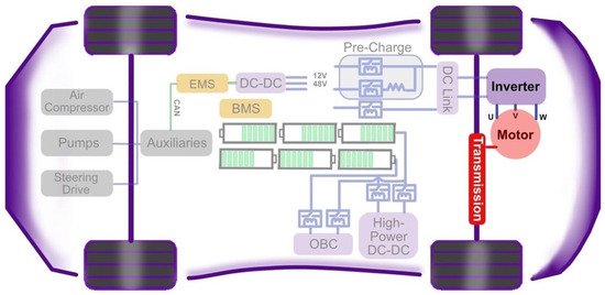
Figure 1.
General architecture of an automotive power drive system (APDS). The high-voltage battery supplies energy through DC/DC converters and a pre-charge circuit to the DC link, which in turn feeds the inverter driving the synchronous traction motor via field-oriented or predictive control algorithms. Auxiliary components such as pumps, compressors, and steering actuators are supplied through dedicated converters. The figure highlights the interplay between energy storage, power conversion, and the traction drive, emphasizing the interfaces where modeling, control, and monitoring strategies are applied.
The electrical energy from the high-voltage battery pack, monitored and managed by the Battery Management System (BMS), is channeled to the DC link via a pre-charge stage. This pre-charge stage limits inrush currents during initial connection, protecting the capacitors and power devices. The DC link acts as an intermediate storage node, stabilizing the voltage and ensuring an instantaneous energy reserve for load fluctuations. From the DC link stage, the energy feeds the inverter, which transforms the DC power into three-phase AC power for the electric motor. The motor, coupled to the mechanical transmission, converts the electrical energy into torque, which is then transferred to the wheels. The efficiency of this process depends on the inverter topology, semiconductor technology, and control strategy, all of which work in close synergy with the cooling system to maintain performance even under heavy loads. In parallel with the traction chain, the system integrates dedicated conversions for auxiliary power supplies. A DC-DC stage reduces the main battery voltage (typically 400 or 800 V) to the levels required for low-voltage services, such as 12 V or 48 V, powering auxiliary devices such as air compressors, pumps, and electric power steering. The Energy Management System (EMS) supervises the distribution and use of energy among the various subsystems, coordinating with the BMS and the inverter control unit via communication buses (e.g., CAN). Battery charging is handled by two distinct conversion paths. The On-Board Charger (OBC) manages charging from the AC grid, converting AC to DC and transferring it to the battery pack. In systems that require it, a High-Power DC-DC converter allows direct charging from high-power DC sources, such as fast charging stations, bypassing the AC-DC stage and reducing energy replenishment times. Overall, this architecture highlights how the APDS is not an isolated block, but a central node in a complex energy ecosystem. Its efficiency and reliability depend not only on the intrinsic quality of its main components, but also on how they interact with energy management systems, charging interfaces, and vehicle auxiliaries. Looking ahead, the integration of advanced control and monitoring algorithms, potentially enhanced by physical models and artificial intelligence techniques, will allow the full potential of each element to be exploited, maximizing the performance of the electric drive system and the lifespan of its components.
The architecture shown can be interpreted as a combination of two overlapping networks: the power network, which transports high- and low-voltage electrical energy, and the information network, which coordinates energy flows and ensures centralized control and operational safety.
On the energy side, the starting point is the high-voltage battery pack, organized into multiple modules connected in series and parallel to achieve the voltage and capacity values required for traction. From the battery pack, energy flows in two main directions: on one side, the DC link, which directly powers the inverter and thus the motor; on the other, the auxiliary and charging branches. Before reaching the DC link, the main path passes through the pre-charging stage, whose function is to prevent inrush currents in the link capacitors and protect the semiconductors during activation. The DC link itself acts as an intermediate storage and filtering node, stabilizing the voltage and providing instantaneous energy for torque transients. From the DC bus, the inverter converts DC power into three-phase AC power and sends it to the electric motor, which transforms the electrical energy into mechanical torque. This torque is transmitted to the wheels through the transmission system, optimizing the engine’s operating speed for different vehicle speeds and loads. In parallel, a conversion branch powers the DC-DC converter dedicated to low-voltage systems. This stage reduces the high voltage of the battery pack to typical levels of 12 V or 48 V, essential for powering auxiliary devices such as air compressors, cooling pumps, and electric steering systems. This is where the Energy Management System (EMS) comes into play, coordinating the distribution of power between traction, auxiliary systems, and charging, constantly communicating with the Battery Management System (BMS) to ensure optimal and safe battery use. On the charging front, the On-Board Charger (OBC) manages the input of power from the AC grid, performing AC/DC conversion and transferring power to the battery pack via the DC bus. In vehicles equipped for ultra-fast charging, a High-Power DC-DC converter allows direct power from DC charging stations, reducing conversion losses and charging times. The second level of the network is the information level. Communication connections, such as the CAN bus, carry commands, monitoring data, and diagnostic signals between the EMS, the BMS, the inverter controller, and the various actuators. This control network ensures that the vehicle’s torque demands are met within safe operating conditions, that charging occurs within thermal and electrical limits, and that any anomalies are promptly detected and managed. Overall, the figure highlights how the APDS is not a simple power-to-traction conversion block, but the core of an interdependent system. Each energy path is controlled by a corresponding communication and supervision chain, and overall performance depends as much on the quality of the components as on the efficiency of these interconnections. The electric drive train in a fully electrified vehicle constitutes the core system responsible for converting stored electrical energy into mechanical torque at the wheels. It can be represented as a functional chain:
Although often described in terms of discrete subsystems, these elements are tightly coupled, with constraints on voltage, current, power, and thermal limits propagating along the chain. Understanding the interaction between them is essential for designing optimal control, ensuring operational safety, and maximizing overall efficiency.
2.2. High-Voltage Battery and BMS Constraints
The high-voltage (HV) traction battery is the primary energy source in the electric drive train, and its accurate modeling is crucial for predicting available power, efficiency, and thermal behavior. A comprehensive overview of HV battery pack design aspects is given in [32], while system-level BMS functions for safety, monitoring, and state estimation are summarized in [33,34]. More recent reviews highlight how modern lithium-ion BMS face stringent constraints in terms of computational feasibility, cell balancing, communication bandwidth, and compliance with safety standards [35,36,37]. Different topologies for centralized, modular, and distributed BMS architectures are compared in [38], showing how voltage levels and modularity affect reliability and diagnostic coverage.
As illustrated in Figure 2, the model integrates electrochemical, electrical, and thermal domains. At the electrochemical level [Figure 2a], lithium-ion transport occurs both in the electrolyte (red arrows) and in the solid active material (blue arrows). These processes determine the open-circuit voltage (OCV) as a nonlinear function of the state of charge (SOC), and they are responsible for voltage relaxation phenomena during transients [33]. The cell’s terminal behavior can be represented by an equivalent electrical model [Figure 2b], consisting of a controlled voltage source in series with an ohmic resistance and one or more RC polarization branches to capture dynamic effects [32]. The SOC dynamics are given by:
where z is the SOC, the battery current (positive during discharge), and the nominal capacity. The terminal voltage is:
with polarization voltages evolving as:
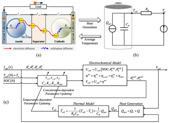
Figure 2.
Multi-domain battery model: (a) electrochemical processes in a lithium-ion cell; (b) equivalent electrical circuit; (c) coupled electrochemical–thermal model with parameter updating and heat generation.
The thermal submodel [Figure 2c] accounts for heat generation as the sum of irreversible Joule losses and reversible entropic heat :
The average cell temperature is described by:
where and are the thermal resistance and capacitance, and is the ambient temperature. The Battery Management System (BMS) continuously monitors , , , and z, enforcing:
The integration of electrochemical, electrical, and thermal models in Figure 2 enables accurate prediction of voltage drop under dynamic load, thermal rise during high current operation, and capacity fade mechanisms [35,37]. The BMS uses this combined model to adjust allowable charge/discharge power in real time, thus directly influencing the maximum torque request that can be sustained by the electric drive [34,36]. Beyond lithium-ion batteries, different chemistries are being considered for automotive drives. Lithium Iron Phosphate (LFP) provides high cycle life and thermal stability but has lower energy density compared to Nickel Manganese Cobalt (NMC) or Nickel Cobalt Aluminum (NCA). Solid-state batteries, although still at an early stage, promise higher safety and energy density by replacing liquid electrolytes with solid ones. These differences strongly affect the performance of the electric drive: NMC and NCA enable longer driving range and higher peak power, whereas LFP offers superior tolerance to regenerative braking cycles thanks to its robustness and stable thermal behavior. The capability of a battery technology to absorb regenerative energy is determined not only by its maximum charge power in (6), but also by thermal constraints and internal resistance. Batteries with lower impedance and higher allowable charging current improve the effectiveness of regenerative braking, reducing the amount of energy dissipated in mechanical braking systems. From an environmental perspective, the choice of battery chemistry influences the full life-cycle impact of the vehicle. NMC and NCA, while offering high specific energy, require critical raw materials such as cobalt and nickel, raising concerns of supply chain sustainability. LFP and future solid-state batteries reduce the dependency on critical elements and are more easily repurposed for second-life applications in stationary storage. Moreover, regenerative braking contributes to lowering the carbon footprint of the vehicle by recovering up to 15–25% of the kinetic energy otherwise lost, thereby reducing net energy demand and indirectly lowering greenhouse gas emissions. This highlights the intertwined role of battery technology, control strategies, and energy recovery in shaping the overall environmental sustainability of automotive electric drives.
2.3. HV-HV DC-DC Converter: Dual Active Bridge (DAB)
In high-performance electric drive trains, an HV-HV DC-DC converter is often inserted between the high-voltage battery and the inverter to regulate the DC-link voltage, optimize modulation range, and decouple the battery dynamics from the fast transients of the motor drive. One of the most widely adopted topologies for this purpose is the Dual Active Bridge (DAB), illustrated in Figure 3.
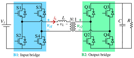
Figure 3.
Dual Active Bridge (DAB) converter topology: (B1) input full-bridge connected to the HV battery; (B2) output full-bridge feeding the DC-link; L is the high-frequency transfer inductance; N is the transformer turns ratio.
The DAB consists of two full-bridge stages: the input bridge (B1, blue) connected to the battery voltage , and the output bridge (B2, green) connected to the DC-link capacitor C and load R. The two bridges are linked by a high-frequency transformer with turns ratio and series leakage inductance L, which serves as the energy transfer element. Both bridges operate with 50% duty cycle square-wave modulation. The control variable is the phase shift between the switching patterns of the two bridges. This phase shift generates an average voltage across the leakage inductance L, producing a power transfer from the primary to the secondary [39,40]. The generalized average modeling (GAM) framework for the DAB is consolidated in [39,41], enabling compact analytical expressions such as those in (8). Extensions to frequency-domain harmonic balance modeling are discussed in [42], while steady-state modeling with circuit parasitics is proposed in [43].
As illustrated in Figure 4, the red trace represents the switched voltage at the primary bridge, while the blue trace is the reflected switched voltage from the secondary bridge. When the two square waves are phase-shifted by , their difference produces a net voltage across L during part of the switching period, causing a triangular current waveform . The inductor current is governed by:
and the average transferred power in ideal operation is:
where n is the transformer turns ratio, the switching angular frequency, and the input and output DC voltages. The input and output currents follow from:
while the DC-link voltage dynamics, including the capacitor C, are:
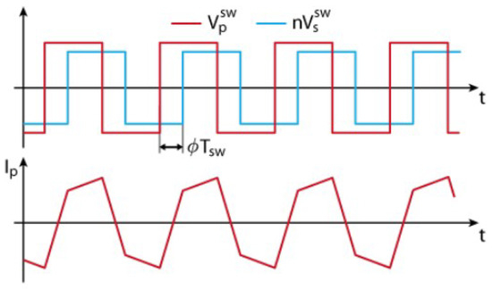
Figure 4.
Voltage waveforms of the primary () and secondary () bridges under phase shift , and resulting inductor current . The phase shift determines the average voltage across L and hence the transferred power.
The phase shift is the key control parameter in the DAB. Increasing raises the overlap area between and , increasing the net voltage across L and thus the power transfer. At , no net energy is transferred, while at the converter operates at maximum power. This phase control enables bidirectional operation: in traction mode, is positive to deliver power from the battery to the DC-link; in regenerative mode, is negative to flow power back to the battery. The design of L must balance soft-switching capability, current ripple, and efficiency. Beyond ideal phase-shift control, several advanced extensions have been proposed. Hybrid modulation strategies that combine single-, dual-, and triple-phase-shift achieve efficiency optimization across load ranges [41,44]. Reviews of topological modifications (multi-port, multi-cell, resonant and hybrid DAB variants) are synthesized in [45], while steady-state and non-ideal AC–DC adaptations are analyzed in [43]. Control-oriented reviews [46] emphasize that model predictive control, feedforward/feedback schemes, and data-driven modulation design [47] are becoming increasingly relevant for automotive-grade HV-HV converters. Collectively, these works establish a robust foundation for DAB deployment but also underline the need for unified models that simultaneously capture soft-switching, losses, and control feasibility in embedded hardware. Although the DAB is the most widespread isolated solution, several other bidirectional converter topologies are employed in automotive electric drives. Non-isolated converters include the interleaved bidirectional buck–boost, the Cuk, SEPIC, and Zeta structures, which are compact and suitable for interfacing auxiliary HV buses or 48 V subsystems. Isolated converters, in addition to the DAB, encompass the bidirectional Phase-Shift Full-Bridge (PSFB), the bidirectional LLC resonant converter, and multiport configurations that enable simultaneous energy exchange among battery, DC link, and on-board charger. Different modeling approaches are applied depending on the topology: state-space averaging and small-signal models for non-isolated converters, generalized average models (GAM) and harmonic balance for DAB and PSFB, and time-domain resonant models for LLC-based converters. These converters play a pivotal role in stabilizing the DC-link voltage during traction and regenerative braking, optimizing efficiency under dynamic driving cycles, and enabling safe bidirectional interaction between the traction battery and the on-board charger. In particular, their ability to handle reverse power flow is essential for maximizing the benefits of regenerative braking and for ensuring reliable fast-charging operations in modern EVs.
2.4. Traction Inverter Topologies and Space Vector Modulation
The traction inverter is the main interface between the high-voltage DC-link and the electric traction motor, synthesizing balanced three-phase AC voltages with controllable magnitude and frequency. The inverter topology and modulation strategy directly influence voltage utilization, harmonic distortion, efficiency, and switching losses. A broad overview of modulation and control techniques for multilevel inverters in traction applications is given in [48], while specific surveys on SVM strategies for NPC and multilevel structures can be found in [49]. Optimized SPWM and carrier-based approaches tailored to traction inverters are discussed in [50], and recent reviews on multiphase traction inverters highlight how modulation and control are evolving with the electrification of heavy-duty and high-power EVs [51]. Beyond reviews, advanced control schemes targeting maximum efficiency across the whole operating range have also been proposed [52], while multiobjective vector modulation tailored to hybrid traction systems has been reported in [53].
Figure 5 illustrates several widely used inverter topologies in electric traction. The conventional two-level VSI is the baseline architecture, while multilevel solutions such as NPC, ANPC, Flying Capacitor, and T-type enable more output voltage levels, reduced THD, and improved efficiency, particularly at high modulation indices [48,49]. Classical two-level SVM techniques are well established and widely documented in the literature. For completeness, we briefly recall that they synthesize the reference voltage vector by time-weighting adjacent active vectors and zero states. In this review we focus instead on recent developments, including multilevel inverters, wide-bandgap device implications, and advanced modulation strategies for automotive applications. In a three-level NPC inverter, each leg can output , 0, or . This expands the set of available vectors from 8 (two-level) to 27 (three-level), providing finer resolution for synthesis [48,49].
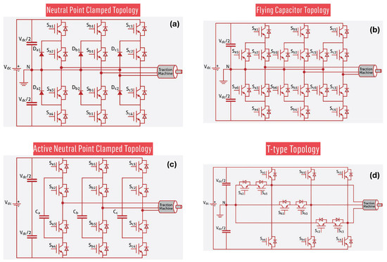
Figure 5.
Common multilevel inverter topologies for traction applications: (a) Neutral Point Clamped (NPC), (b) Flying Capacitor (FC), (c) Active Neutral Point Clamped (ANPC), and (d) T-type. Multilevel structures increase the number of output voltage levels, reduce harmonic content, and lower device stress.
Figure 6 shows that each main sector is split into sub-sectors. For a given , the modulation algorithm selects the two nearest active vectors and one zero or medium vector from the available set. The voltage step for an m-level inverter is:
For , . The generalized duty cycle calculation is:
where are the angles of the selected active vectors.
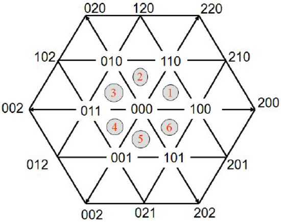
Figure 6.
Space vector diagram for a three-level inverter: Each main sector is subdivided into four sub-sectors. The sub-sector location determines the set of active and zero vectors used in the synthesis.
Remarks on Multilevel SVM:
- Neutral Point Balancing: NPC and ANPC topologies require control of neutral point voltage to avoid imbalance between DC-link capacitors [48,49].
- Flying Capacitor Balancing: FC topologies need periodic modulation adjustments to maintain capacitor voltages [48].
- T-type Loss Reduction: T-type legs reduce conduction path length for zero voltage states, lowering switching and conduction losses [48,51].
By increasing the number of levels, multilevel SVM reduces Total Harmonic Distortion (THD), lowers device voltage stress , and improves efficiency, which is critical in high-performance EV traction applications [50,52,53].
2.5. Synchronous Motor Modeling for Automotive Traction
In modern electric vehicles, synchronous machines represent the most efficient choice for traction applications. Compared to induction machines, synchronous motors can achieve higher power density, superior peak efficiency, and better controllability, especially when paired with advanced control strategies such as Field-Oriented Control (FOC) or Model Predictive Control (MPC). Their ability to maintain high efficiency over a wide torque-speed range, combined with reduced rotor losses, makes them ideal for high-performance automotive use [54,55,56,57,58,59,60]. The general three-phase model of a synchronous machine neglecting space harmonics and assuming sinusoidal distributed windings is:
where , , and () are the phase voltages, currents, and flux linkages, and is the stator resistance [58]. The flux linkages can be expressed as:
where is the position-dependent inductance matrix and are the flux linkages due to permanent magnets [54]. For control purposes, the model is transformed into orthogonal reference frames using Clarke and Park transformations [60].
where is the electrical rotor angle. Applying these transformations to the model yields the well-known Park-frame equations:
The electromagnetic torque is:
where p is the number of pole pairs, the permanent magnet flux linkage, and , are the inductances along the direct and quadrature axes [58,59]. Automotive traction employs several variants of synchronous machines, each with specific characteristics [54,55,57,58]:
- Surface-mounted Permanent Magnet Synchronous Machine (SPMSM): Permanent magnets are mounted on the rotor surface, resulting in a nearly isotropic rotor (equal and ). This design provides high torque density and a simple electromagnetic model, but limited field-weakening capability due to high back-EMF.
- Interior Permanent Magnet Synchronous Machine (IPMSM): Magnets are embedded within the rotor, introducing rotor saliency () and enabling reluctance torque production in addition to magnet torque. IPMSMs exhibit excellent field-weakening performance and high efficiency over extended speed ranges.
- Synchronous Reluctance Machine (SynRM): Torque is produced solely by rotor saliency without magnets (). While efficiency is lower than PMSM at low speed, SynRMs eliminate rare-earth materials and offer robust high-speed operation. Their magnet-free design makes them particularly attractive in the context of circular economy and sustainability, since they avoid the use of critical raw materials such as neodymium and dysprosium. Recent research has focused on advanced rotor barrier design, ferrite-assisted reluctance machines, and optimization techniques that improve torque density and efficiency, thereby bridging the gap with PMSMs while retaining environmental and cost advantages.
- Hybrid PM-SynRM: Combines permanent magnets and reluctance torque to balance cost, efficiency, and field-weakening capability.
The choice of synchronous motor topology directly affects the parameters of the Park model [54,55,57,58]:
- SPMSM: , torque production relies mainly on . Field-weakening is limited since .
- IPMSM: , reluctance torque significantly contributes to , enhancing torque per ampere and field-weakening performance.
- SynRM: , torque is purely reluctance-based, requiring for positive torque production. In addition to their simplified model structure, SynRMs are less sensitive to permanent magnet degradation phenomena (e.g., partial demagnetization), which enhances robustness in long-term operation. This intrinsic resilience further strengthens their position as a promising rare-earth-free alternative for future EV powertrains.
- Hybrid PM-SynRM: Intermediate and moderate saliency combine both PM and reluctance torque contributions.
While the classical -axis model accurately captures the electromechanical energy conversion in synchronous machines under idealized conditions, high-fidelity models for automotive applications must also include secondary torque components and friction phenomena that significantly affect performance, especially at low speed or during high dynamic torque demands [58,59]. Cogging torque, also referred to as detent torque, arises from the interaction between rotor permanent magnets and the stator slots, even when no current flows in the stator windings. This torque is position-dependent and periodic with respect to the mechanical rotor angle :
where is the number of stator slots, p the number of pole pairs, and the amplitude and phase of the h-th harmonic component, and the number of harmonics retained in the model. The cogging torque is superimposed on the electromagnetic torque, modifying the total torque equation as:
The Stribeck effect models the nonlinear behavior of friction torque at low speeds, where static friction and viscous friction interact with the boundary lubrication regime [59].
Incorporating both cogging torque and Stribeck friction into the mechanical equation of the -model yields:
The presence of and Stribeck friction necessitates advanced compensation strategies:
- Feedforward cogging torque cancellation based on rotor position estimation.
- Adaptive friction compensation in speed and torque controllers, especially for smooth creep and launch control in EVs.
- Enhanced observers in FOC or MPC schemes to estimate disturbance torque in real-time and adjust current references accordingly.
These enhancements ensure that the model and control system reflect the real-world behavior of the machine under all operating conditions, from standstill to high-speed operation [58,59,60].
It is important to remark that the parameters of the synchronous machine model (, , , ) are not constant, but vary significantly with temperature, magnetic saturation, and long-term aging. These variations introduce model uncertainties that affect torque prediction and current control accuracy. Robust design therefore requires monitoring and adaptive estimation of such parameters, together with control strategies capable of guaranteeing performance under bounded uncertainty.
3. Advanced Control Strategies for Synchronous Motor Drives
The high-performance requirements of automotive synchronous drives demand control strategies that go beyond classical approaches. Among the advanced techniques investigated are feedback linearization, model predictive control, sliding mode control, adaptive data-driven methods, and reinforcement learning. Each of these strategies exploits the affine-in-input structure of the PMSM/IPMSM model in Park coordinates, where with and , and where torque, inverter voltage, and thermal constraints appear as algebraic maps or feasibility sets. We now present each control approach in detail, combining mathematical rigor with implementation considerations. Beyond their theoretical formulation, the application of advanced control strategies to automotive electric drives requires a structured design methodology. The key steps can be summarized as follows:
- Feedback Linearization: The methodology involves (i) selecting outputs that provide full state feedback, (ii) verifying the nonsingularity of the decoupling matrix , (iii) computing the feedback law , and (iv) tuning the gain matrix K to place the poles of the linearized error dynamics.
- Model Predictive Control (MPC): The design requires (i) deriving a discrete-time prediction model , (ii) formulating a cost function that balances torque tracking, flux regulation, and switching losses, (iii) defining the feasibility set and state constraints (currents, temperatures), (iv) selecting prediction horizon and weights , and (v) implementing an optimization solver compatible with embedded execution.
- Sliding Mode Control (SMC): The methodology starts with (i) defining a sliding surface , (ii) ensuring the reachability condition , (iii) computing the equivalent control , (iv) designing the discontinuous term with robustness margins against uncertainty, and (v) mitigating chattering through boundary layer design or higher-order algorithms (e.g., super-twisting).
- Adaptive Control: The design procedure includes (i) specifying a reference model , (ii) deriving the adaptation law , (iii) ensuring stability via Lyapunov analysis with positive-definite P, (iv) validating the persistent excitation (PE) condition or employing concurrent learning/DREM methods, and (v) tuning adaptation gains to balance convergence speed and robustness to noise.
- Reinforcement Learning (RL): The methodology is based on (i) defining the Markov Decision Process (state, action, transition, reward), (ii) shaping a reward function that encodes torque tracking, efficiency, and thermal constraints, (iii) training the policy offline using high-fidelity simulations with domain randomization, (iv) validating the learned controller under safety layers that enforce admissibility of , and (v) deploying a lightweight inference network on the embedded drive controller.
These methodologies highlight how each strategy requires a balance between rigorous mathematical derivation and practical implementation choices. The emphasis is on ensuring stability, robustness, and feasibility on automotive-grade hardware while respecting functional safety requirements.
3.1. Feedback Linearization
Feedback linearization aims to transform the nonlinear PMSM/IPMSM dynamics into a linear, decoupled system by algebraically canceling the cross terms and speed-dependent nonlinearities. Starting from the Park-frame equations introduced earlier, the current dynamics can be written in affine-in-input form as
where
The outputs are chosen as , so that
The decoupling matrix E is diagonal with strictly positive entries (, ), and therefore always nonsingular as long as , a condition met in any practical PMSM/IPMSM. One can thus impose the virtual input
and define the feedback linearizing control law
By substitution into the closed-loop system, the error obeys
which guarantees exponential convergence. To formally prove stability, consider the Lyapunov candidate , yielding . If K is symmetric positive definite or has symmetric part , then , proving global exponential stability [61,62]. From a formal point of view, feedback linearization belongs to the family of input–output linearization techniques. Given a nonlinear system of the form , the existence of a diffeomorphism such that the dynamics in the new coordinates are linear depends on the relative degree of the outputs and on the nonsingularity of the decoupling matrix . In the PMSM/IPMSM case, since is always nonsingular, the system admits an exact linearizing transformation. The closed-loop dynamics can be written explicitly as
so that z behaves as a pair of decoupled integrators driven by . This guarantees that the feedback-linearized system is not only linear but also controllable, and any classical linear control technique (pole placement, LQR, PI/PID tuning) can be directly applied to shape the error dynamics. In practice, exact cancellation is never achieved because parameters and the angle are uncertain or slowly drifting with temperature, saturation, and aging. Suppose the actual dynamics differ by and from the nominal ones used in (28); the error dynamics become
where is a bounded disturbance due to modeling errors. By choosing an additional corrective term in the law, one achieves input-to-state stability. Specifically, with we obtain
so that if the error remains bounded and converges to a neighborhood of the origin proportional to the uncertainty bound . This establishes robustness margins [63,64]. The block diagram in Figure 7 provides an intuitive view of the method: the original nonlinear system is mapped through a nonlinear coordinate transformation and inverted by the feedback law, such that the overall closed loop behaves like a linear system controlled by a conventional linear regulator. In this way, the sophisticated algebra embedded in (28) reduces to a structure where standard PI or pole-placement design can be used once the nonlinear dynamics are canceled [65,66].
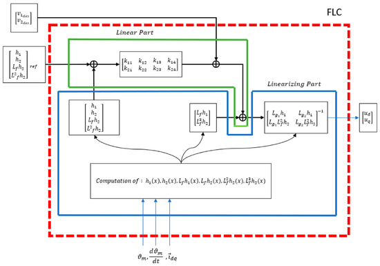
Figure 7.
Detailed architecture of the feedback linearization controller (FLC) for PMSM/IPMSM drives. The Linearizing Part (blue box) computes the Lie derivatives of the outputs up to the second order, as well as the decoupling matrix , thereby canceling the nonlinear cross-couplings of the machine model. The Linear Part (green box) introduces the virtual control input through a gain matrix K, enforcing the desired closed-loop dynamics. The overall scheme (red dashed box) transforms the nonlinear PMSM/IPMSM dynamics into two decoupled integrator chains, so that conventional linear control design techniques (PI tuning, pole placement) can be directly applied.
From an implementation perspective, feedback linearization is computationally light, as it requires only matrix inversion (trivial in the diagonal case) and a few multiplications per sampling period. On a typical DSP running at 100–200 MHz, the additional load is negligible compared to SVPWM generation. The main challenge lies in sensorless operation: accurate rotor angle estimation is mandatory, since any phase error in directly compromises decoupling. Extended Kalman Filters (EKF) or Unscented KFs are used at medium and high speed, while high-frequency injection is employed near zero speed. In production systems, look-up maps and online estimators provide and values to compensate parameter drift. Furthermore, actuator constraints such as voltage saturation in the SVM region must be respected: in practice, (28) is combined with a projection onto . Finally, because the approach cancels natural dynamics, measurement noise can be amplified; filtering strategies and observer-based implementations are essential to ensure robustness in an embedded automotive controller [67,68]. In summary, feedback linearization provides a rigorous framework in which the nonlinear PMSM/IPMSM dynamics are formally transformed into a linear, controllable system. The explicit construction of the diffeomorphism and the nonsingularity of the decoupling matrix ensure the validity of the approach, while Lyapunov analysis certifies stability of the closed-loop dynamics. This mathematical foundation justifies the practical application of classical linear control strategies in automotive electric drives, combining theoretical rigor with implementation feasibility.
3.2. Model Predictive Control
Model predictive control represents one of the most systematic frameworks for current and torque regulation in synchronous motor drives, as it explicitly accounts for system dynamics, constraints, and performance indices in a unified optimization problem solved at every sampling instant [69,70,71]. Starting from the affine-in-input representation , the discretized model under zero-order hold is expressed as
where the matrices capture the electrical dynamics over the sampling period , and d represents the known disturbance due to the back-EMF term proportional to . The inverter feasibility set is given by the hexagonal voltage limit induced by space vector modulation, while the admissible state set encodes current and thermal constraints. The generic architecture of MPC is illustrated in Figure 8, where the prediction model forecasts the machine response over the horizon, and the optimizer computes the control input that minimizes a given cost function while satisfying constraints. The block diagram highlights the three pillars of MPC: the cost function defining the performance objective, the constraints representing feasibility and safety, and the prediction model that links future control actions to system evolution.
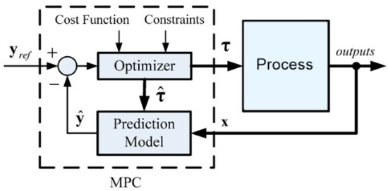
Figure 8.
Schematic architecture of model predictive control: the optimizer computes the optimal input by minimizing a cost function subject to constraints, using a prediction model of the process.
The standard finite-horizon MPC problem is formulated as
This is a quadratic program (QP) with linear dynamics and convex quadratic cost. Convexity ensures the existence of a unique global minimizer, which can be found efficiently by active-set or interior-point algorithms tailored for embedded processors. The optimality conditions follow from the Karush–Kuhn–Tucker (KKT) framework. Denote by the decision variables and by the predicted states. The Lagrangian is
where are inequality constraints (currents, voltages, thermal limits) and the equality dynamics. The KKT conditions then require: stationarity , primal feasibility , dual feasibility , and complementary slackness . In practical implementations, solvers exploit the sparse block structure of to achieve computational efficiency. Closed-loop stability is ensured by augmenting the cost with a terminal penalty and restricting the terminal state to a set invariant under a stabilizing local controller. This guarantees that the cost-to-go functions as a Lyapunov function, decreasing along closed-loop trajectories [72]. A key distinction lies between continuous-input MPC and finite-control-set MPC. In continuous MPC, the decision variable is the continuous voltage vector, and the solution of the QP yields an optimal that is then synthesized by SVPWM. This approach provides smooth currents and low THD but requires solving a QP every , with computational complexity where . In finite-control-set MPC, by contrast, the admissible are restricted to the finite set of inverter switching vectors (7 nonzero vectors for a 2-level inverter, 19 for a 3-level NPC). The cost is evaluated for each candidate, and the minimizer is directly applied to the switches, eliminating the modulation stage. This drastically reduces complexity but introduces current ripple due to the coarse nature of the input set [73,74]. Implementation practice in automotive drives reflects these trade-offs. Continuous-input MPC has been demonstrated in hardware-in-the-loop platforms using custom FPGA accelerators, with sampling times down to s, exploiting pipelined interior-point solvers [69,70]. Finite-control-set MPC is computationally much lighter, requiring only a few multiplications per candidate vector, and is therefore feasible on conventional DSPs with –s. However, ripple management is critical, and multi-step horizons or switching-frequency penalization are often added to smooth performance. Sensorless operation integrates naturally: moving horizon estimation (MHE) uses the same predictive model and optimization machinery to jointly estimate and , ensuring coherence between observer and controller. In production prototypes, however, lighter Luenberger or extended Kalman observers are preferred to reduce complexity, with MHE reserved for high-performance demonstrators [71]. Tuning the weights is crucial: large enforces accurate torque tracking, while manages flux or field weakening, and penalizes switching effort to reduce losses. Industrial practice often limits the horizon to or 2 for real-time feasibility. More advanced schemes embed electro-thermal constraints by adding junction temperature predictions from reduced-order thermal models to the inequality set , thereby achieving constraint-aware derating [75,76]. This makes MPC uniquely suited for multi-domain optimization in next-generation EV traction inverters.
3.3. Sliding Mode Control
Sliding Mode Control (SMC) is a robust nonlinear control methodology that exploits the discontinuous nature of the control input to force the system trajectory onto a chosen manifold and maintain it there despite disturbances and parameter uncertainties. For PMSM/IPMSM current regulation, let the tracking error be and define a sliding surface as a linear combination of the errors, namely
where is a positive diagonal matrix. The control objective is to drive in finite time and then maintain it at zero, implying under nominal dynamics [77,78]. The block diagram in Figure 9 illustrates the essential structure of SMC. The system output is compared with its reference to form the sliding variable ; this is then fed into a discontinuous control law that switches the input to ensure convergence of . The figure also emphasizes the role of the system dynamics in shaping the equivalent control , while the discontinuous term enforces robustness.
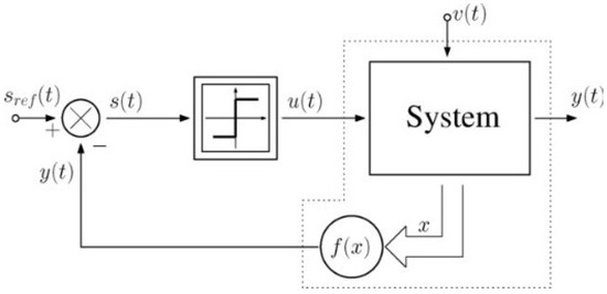
Figure 9.
Block diagram of Sliding Mode Control. The reference signal is compared with the measured output to generate the sliding variable . The equivalent control is computed from the nominal model so as to satisfy , while the discontinuous term guarantees robustness against parameter uncertainties and disturbances. Once , the closed-loop dynamics evolve on the sliding manifold, effectively reducing the nonlinear PMSM/IPMSM system to a robust linear subsystem.
The equivalent control is defined as the continuous input that would keep under the nominal model . Substituting this into yields
Formally, the SMC design is based on two conditions: (i) the reachability condition, which requires that the system trajectory is driven towards the manifold , and (ii) the invariance condition, which ensures that once is reached, the trajectory remains on it. The reachability condition is guaranteed if there exists such that
This ensures that the manifold is attractive. The invariance condition follows from when the equivalent control is applied, proving that the reduced-order dynamics evolve entirely on the sliding surface. In practice, uncertainties prevent exact cancellation, so a discontinuous term is added:
where is a gain matrix, is a smoothed signum, and defines a boundary layer. This ensures robustness. To show finite-time convergence, consider the Lyapunov function . Its derivative is
Substituting the control law gives
where bounds the model uncertainty. If K is chosen such that , then whenever , proving finite-time convergence of . Once on the sliding surface, the dynamics reduce to , which correspond to the nominal linearized current loops, hence ensuring robust tracking [79,80]. An alternative proof of finite-time convergence can be obtained by integrating the inequality to show that reaches the manifold in a settling time upper-bounded by
This explicit bound on the convergence time is particularly useful for automotive applications, where the transient duration directly affects driveability and safety. However, the discontinuous term generates high-frequency switching known as chattering, which produces current ripple, additional losses, and acoustic noise. To mitigate this, higher-order sliding mode algorithms are adopted. Among them, the super-twisting algorithm is widely used. It defines the input derivative as
with positive gains chosen according to Lipschitz bounds of the error dynamics. The associated Lyapunov analysis uses to show that both S and converge to zero in finite time, while u remains continuous. This eliminates high-frequency chattering while preserving robustness, a crucial feature for automotive drives [78,81]. In summary, SMC formally guarantees robustness against matched uncertainties by enforcing sliding dynamics on a carefully designed manifold . The reachability and invariance conditions, together with Lyapunov-based convergence proofs, provide a rigorous mathematical justification. Practical implementations require engineering trade-offs: boundary layers and super-twisting mitigate chattering, while careful gain tuning ensures fast convergence without excessive stress on the inverter. From the implementation viewpoint, SMC is computationally inexpensive, requiring only evaluation of the sliding variable, equivalent control, and a discontinuous or super-twisting update law. This makes it suitable for DSP-based controllers with sampling times of tens of microseconds. Nevertheless, careful tuning is required: gains that are too low fail to overcome uncertainty, while excessive gains amplify ripple and stress the inverter. Practical implementations employ a saturation function to soften the discontinuity, and add low-pass filters or predictive ripple compensation to further reduce torque pulsations. For sensorless operation, SMC pairs naturally with sliding mode observers (SMO) that estimate rotor flux and angle by exploiting the same discontinuous structure; in practice, SMOs are combined with high-frequency injection or fuzzy/terminal observers to improve performance at standstill [82,83,84]. Overall, sliding mode control offers unmatched robustness to parameter variations and disturbances, but its integration in EV drives requires engineering solutions to manage ripple, acoustic noise, and interaction with electro-thermal constraints [85].
3.4. Adaptive Data-Driven Control
Adaptive control addresses the fundamental limitation of fixed-parameter model-based strategies, namely their sensitivity to parameter variations due to temperature, magnetic saturation, or long-term aging of the machine. Instead of relying on static parameter identification, adaptive controllers continuously update their gains based on real-time measurement data, ensuring consistent performance across operating conditions. In the context of PMSM/IPMSM drives, a widely used framework is Model Reference Adaptive Control (MRAC), in which the drive currents are required to follow the dynamics of a desired reference model [86,87,88]. Let the reference model be , where represents the reference dynamics and r is a reference input (typically related to the torque demand). The actual machine dynamics in compact affine form are , with capturing unmodeled effects and parameter uncertainty. The adaptive control law is chosen as
where is a regressor vector (constructed from currents and reference signals) and K is the adaptive gain matrix to be updated online. Defining the model tracking error , the adaptation law is
with the adaptation gain matrix, P the solution of the Lyapunov equation , and . The stability of MRAC can be formally established. Consider the Lyapunov function candidate
where is the parameter estimation error with respect to the ideal gain matrix that achieves perfect model matching. Differentiating V along the system trajectories and substituting the update law yields
which shows global stability and convergence of . Thus, the adaptive law guarantees asymptotic tracking of the reference model under nominal conditions. The block diagram in Figure 10 provides a visual summary of this principle: the controlled system is forced to track a reference model by adjusting the adaptive input , which compensates the uncertainty via the disturbance model . The adaptation loop continuously updates the parameters K based on the error between the reference and the actual system, enforcing the desired closed-loop dynamics.
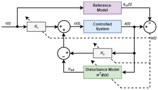
Figure 10.
Block diagram of a Model Reference Adaptive Control (MRAC) scheme: the adaptive input updates the control law in real time to minimize the tracking error , forcing the controlled system to follow the reference model despite disturbances and parameter variations.
However, a critical requirement for parameter convergence is the so-called Persistent Excitation (PE) condition, namely that for some finite T. In automotive duty cycles, excitation may be weak or insufficient due to long periods of nearly constant operating points. To overcome this, modern adaptive schemes employ Concurrent Learning (CL), where recorded data are stored in a memory stack and re-used to excite the regressor space even in the absence of instantaneous PE. The adaptation law is then augmented with an additional term proportional to the parameter error evaluated at past data points. Another powerful method is Dynamic Regressor Extension and Mixing (DREM), which uses filtering and regressor transformations to extract richer excitation from the available signals, thereby ensuring parameter convergence without persistent input variation [89,90,91,92]. Both CL and DREM are compatible with embedded implementation, as they rely on simple algebraic extensions of the update law. From a practical standpoint, adaptive control is computationally lightweight compared to MPC, since it requires only vector-matrix multiplications and parameter updates at each sampling step. This makes it well-suited to DSP-based control units with sampling times in the range of –s. The main implementation challenge lies in tuning the adaptation gain : if chosen too small, convergence is slow and performance drifts under parameter variations; if too large, oscillations or even instability may occur in the presence of measurement noise. In practice, projection operators are used to bound K within safe intervals, preventing runaway adaptation. Moreover, adaptive controllers are often combined with observers: neural network observers (RNN, GRU, or LSTM based) can provide estimates of rotor angle and speed , while adaptive KFs fuse these data-driven estimates with physical models [87,88]. This hybrid approach exploits the adaptability of data-driven methods while retaining the interpretability of physics-based observers. In automotive prototypes, adaptive data-driven control has shown promise in handling electro-thermal coupling: by augmenting the regressor vector with estimated junction temperatures or saturation indicators, the adaptation law implicitly compensates multi-domain interactions, making this method attractive for next-generation electric drives [93].
3.5. Reinforcement Learning
Reinforcement Learning (RL) constitutes the most flexible framework among advanced control strategies, as it does not require an explicit analytic controller but instead learns an optimal decision policy through interaction with the environment. The PMSM/IPMSM drive is naturally cast as a Markov Decision Process (MDP), defined by a state space , an action space , a stochastic transition function describing the machine dynamics, and a reward function that quantifies the control objectives [94,95]. At each sampling instant k, the controller observes a state , which can include electrical currents , mechanical states , estimated junction temperature , and additional features from observers, and then selects an action corresponding to inverter commands (either continuous voltages or discrete switching vectors in finite-control-set RL). The environment transitions to according to , and the agent receives a scalar reward . The objective is to maximize the expected discounted return
where is the policy mapping states to action distributions, and is the discount factor [96]. The theoretical foundation is the Bellman optimality equation for the state-action value function
which characterizes the cumulative reward starting from under policy . Optimal control corresponds to finding [97]. In policy gradient methods, the parameters of a stochastic policy are updated by
which follows from the likelihood ratio trick. To reduce variance, actor–critic architectures introduce a critic estimating the advantage , yielding the practical update
Popular implementations include Proximal Policy Optimization (PPO) and Soft Actor–Critic (SAC), both compatible with continuous or discrete inverter action sets [98]. The block diagram in Figure 11 illustrates the RL loop applied to electric drives. The agent (policy) selects actions based on the observed state , applies them to the environment (the motor-inverter system), and receives both the next state and a scalar reward . The reward encapsulates the control objectives (torque tracking, efficiency, safety), and the policy is updated accordingly. This closed loop of interaction and learning highlights the data-driven nature of RL, contrasting with model-based schemes.
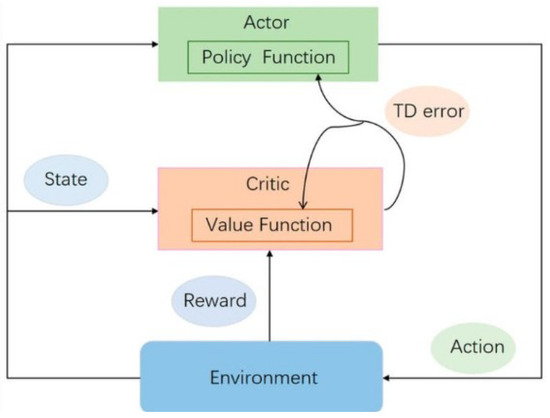
Figure 11.
Reinforcement learning control architecture: the agent (policy) interacts with the environment (motor + inverter) by observing the state s, applying action a, and receiving a reward r, which encodes the control objectives.
The reward is the key design element and directly encodes multi-domain objectives. A representative example is
where the terms penalize torque tracking error, electrical losses, thermal limit violations, and infeasible voltage commands. In this way, RL inherently handles electro-mechanical, electro-thermal, and inverter feasibility objectives without the need for explicit model equations in the controller. Extensions also allow penalizing current ripple or acoustic noise, making RL a candidate for integrated NVH optimization [99,100]. From a stability viewpoint, RL does not provide analytical guarantees comparable to model-based methods; however, if the critic converges, the learned policy approximates the optimal solution to the Bellman equation. Practical safety requires augmenting the learned policy with projections or safety layers: at runtime, the action suggested by the neural policy is projected onto the admissible set , and control barrier functions ensure that state constraints (currents, temperatures) remain invariant sets [96,97]. Implementation in automotive drives follows a two-phase approach. Training is typically performed offline in a high-fidelity simulator that includes electromagnetic and thermal models, and training strategies such as domain randomization are applied to expose the agent to a wide distribution of parameters and non-idealities of the inverter. This enhances robustness for sim-to-real transfer [98]. Deployment consists of embedding the trained neural network policy, which has modest inference cost (a few matrix multiplications), into the DSP/FPGA of the drive controller, with safety layers ensuring hard constraint satisfaction. Sensorless operation can be embedded directly in the policy network by providing histories of as inputs, letting the latent representation encode , or by coupling the policy with classical EKF/MHE observers to ensure interpretability and reliability [95,101]. In summary, reinforcement learning provides unmatched flexibility to incorporate arbitrary control objectives and naturally accommodates multi-domain optimization. Yet, the absence of closed-form guarantees, the heavy data requirements for training, and the challenges of certification and safety represent the main barriers to its deployment in safety-critical automotive environments [99,100].
3.6. Intelligent Control Strategies
The increasing complexity of automotive electric drives has motivated the adoption of intelligent control strategies that integrate machine learning, artificial intelligence, and knowledge-based methods into the control loop. These approaches differ from classical advanced controllers in that they can exploit data-driven models, nonlinear approximators, and adaptive decision-making frameworks to improve robustness, adaptability, and performance in uncertain or highly variable operating conditions. Artificial Neural Networks (ANNs) are widely employed as nonlinear function approximators that can map system states to control actions. In PMSM/IPMSM drives, multilayer perceptrons and recurrent architectures (e.g., LSTM, GRU) have been used to estimate torque-producing currents or to generate optimal voltage commands under varying operating conditions. The training phase is typically performed offline using high-fidelity motor–inverter models or experimental datasets, while online inference is lightweight enough to be embedded in DSP/FPGA hardware. Stability is usually analyzed through Lyapunov-based adaptive laws that ensure boundedness of the estimation error [102,103,104,105,106]. Fuzzy logic controllers provide an interpretable rule-based framework that can encode expert knowledge of the drive dynamics. In automotive applications, fuzzy controllers have been applied to torque control, flux weakening, and regenerative braking management. Hybrid neuro-fuzzy systems combine the transparency of fuzzy rules with the learning capability of neural networks, allowing automatic tuning of membership functions and rule weights. This results in improved adaptability to nonlinearities and parameter drifts [107,108,109]. Several studies have proposed integrating intelligent methods with classical control structures. For example, neural networks can be employed to adaptively tune the gains of sliding mode controllers, reducing chattering while preserving robustness. Similarly, reinforcement learning agents can be combined with predictive models to create hybrid model-based/model-free architectures that achieve both stability guarantees and adaptability. Other hybrid approaches include AI-assisted parameter scheduling for MPC cost functions or neural observers fused with Kalman filters for sensorless operation [110,111,112,113]. Intelligent controllers provide enhanced adaptability to parameter variations, the ability to handle unmodeled nonlinearities, and potential for multi-objective optimization (e.g., torque tracking, efficiency, NVH reduction). However, their integration into safety-critical automotive systems is still limited by challenges such as computational burden, the need for extensive training datasets, lack of interpretability, and certification under functional safety standards (ISO 26262). Ongoing research addresses these issues through physics-informed neural networks, safety layers, and quantization/distillation techniques to reduce model complexity. In summary, intelligent control strategies complement classical advanced methods by providing data-driven adaptability and knowledge-based decision-making. Their role is expected to grow in next-generation automotive electric drives, particularly in scenarios where robustness to uncertainty, seamless integration with monitoring frameworks, and multi-domain optimization are critical.
3.7. Comparative Discussion
The five advanced control methods presented cover a wide spectrum of philosophies and trade-offs, from exact algebraic cancellation to optimization-based decision-making and fully data-driven policies. Feedback linearization and sliding mode control share the goal of robustifying the nonlinear PMSM/IPMSM dynamics, yet they differ in their approach: the former aims at decoupling and reducing the system to a linear model but suffers from parameter sensitivity, while the latter embraces the uncertainties and guarantees finite-time convergence at the price of ripple and chattering. Model predictive control and reinforcement learning represent optimization-based paradigms, with MPC providing explicit guarantees through convex optimization and constraints, and RL relying on data-driven exploration and reward shaping to achieve flexibility, albeit without formal stability proofs. Adaptive data-driven control lies between these extremes, offering continuous online adjustment to parameter drift while retaining interpretability and relatively low complexity. Beyond these classical advanced methods, intelligent control strategies introduce a further paradigm shift. Neural network controllers can approximate unknown nonlinearities and adapt control actions to changing drive conditions; fuzzy and neuro-fuzzy approaches embed expert knowledge into interpretable rules, with adaptive tuning provided by learning algorithms; hybrid intelligent controllers exploit neural or fuzzy layers to adjust the parameters of MPC or SMC online, combining analytical guarantees with adaptability. Such methods are increasingly explored in automotive contexts for torque tracking, flux weakening, and regenerative braking optimization. From a practical automotive viewpoint, the key discriminants are computational feasibility, sensorless integration, and multi-domain capability. Feedback linearization is extremely light computationally and attractive for embedded DSPs, but it requires high-fidelity observers for . MPC is systematic and integrates electro-thermal limits explicitly, but its QP solving load makes it suitable only for platforms with dedicated accelerators or heavily simplified formulations. Sliding mode control is simple to implement and robust, yet the mitigation of chattering is a non-trivial engineering task, particularly when NVH constraints are stringent.
Adaptive controllers are appealing for lifetime robustness, since they track slow thermal and magnetic drifts, but their reliance on persistent excitation or stored data raises questions on identifiability under typical drive cycles. Reinforcement learning is in principle the most general, capable of shaping arbitrary objectives including efficiency, comfort, and safety; however, the data and training requirements, the lack of closed-form guarantees, and the certification challenges under ISO 26262 currently limit its adoption to research prototypes. Intelligent controllers, while still at an earlier stage of industrial deployment, add new dimensions to this comparison. Their main advantages are the capability to handle multi-domain objectives natively, adaptability to unmodeled dynamics, and the possibility of incorporating human expertise through rule-based or hybrid structures. Their weaknesses include high training effort, potential lack of transparency, and difficulties in functional safety certification. Physics-informed neural networks, digital twins enriched with AI correctors, and safety-shielded learning are among the emerging solutions to bridge these gaps. It is also worth noting that hybrid schemes are actively explored: adaptive MPC uses online parameter updating to preserve predictive accuracy; SMC with adaptive or neural gains reduces chattering; RL with embedded model knowledge (model-based RL) increases sample efficiency; and FBL layers combined with outer MPC loops can provide both light computation and constraint enforcement. In this landscape, intelligent control strategies play an enabling role, providing data-driven adaptability and optimization capabilities that can be layered on top of model-based methods. Future automotive drives are thus expected to rely on hybrid architectures that integrate rigorous analytical controllers with intelligent learning-based modules. The comparative landscape therefore suggests that the future of automotive drives will not rely on a single paradigm, but rather on carefully engineered combinations that exploit the strengths of each. Table 3 summarizes the main properties of the discussed methods, including their flexibility, computational demand, sensorless integration capability, multi-domain extension, and robustness. The table has been formatted to automatically adapt to the page width for readability.
Table 3.
Comparison of advanced and intelligent control strategies for PMSM/IPMSM drives.
4. Monitoring in Automotive Electric Drives
The monitoring of automotive electric drives represents a cornerstone for ensuring safety, reliability, and durability of the entire traction system. Unlike classical approaches where monitoring was understood merely as the acquisition of basic electrical signals such as currents and voltages, modern requirements extend the concept towards a comprehensive framework that encompasses the continuous supervision of electrical, thermal, magnetic, and mechanical states, together with the prediction of their evolution in time and the detection of incipient faults. In other words, monitoring in contemporary PMSM and IPMSM drives is no longer restricted to being a support tool for control, but has evolved into an integrated diagnostic and prognostic layer that sustains the overall health management of the drive, fully aligned with the paradigm of Prognostics and Health Management (PHM). A first class of monitoring challenges concerns the electrical domain. The three-phase structure of the PMSM/IPMSM implies that monitoring must continuously assess the integrity of the phase currents , , and of the corresponding voltages, which after Clarke and Park transformations enter directly into the control law. Failures in current sensors, offsets, saturation, or loss of one phase connection lead to deviations in the reconstructed state vector and, consequently, in the estimated torque . Moreover, semiconductor failures in the inverter such as open-circuit or short-circuit faults alter the mapping between the control input and the actual applied voltages, thereby introducing nonlinear distortions that the monitoring system must recognize in real time. The detection of such faults typically relies on residual generation, where the measured are compared against the expected behavior produced by the nominal model , and the residual is continuously evaluated. Small but systematic deviations in r are indicative of sensor bias, while abrupt changes are symptomatic of inverter faults or wiring issues. Another crucial dimension is thermal monitoring. Excessive temperatures in stator windings, permanent magnets, and semiconductor junctions are the primary cause of accelerated aging, insulation breakdown, and irreversible demagnetization. The main challenge is that direct sensing is feasible only at limited points, for instance with NTC thermistors on the winding heads or embedded diodes in IGBT modules, while the true critical temperatures occur in locations where sensors cannot be mounted, such as the midpoint of the winding or the MOSFET die. For this reason, thermal monitoring must combine direct measurements with reduced-order thermal models, typically of RC-network type, which approximate the heat conduction path as a set of differential equations of the form , where and denote thermal capacitance and conductance matrices, and is the vector of heat sources due to copper and iron losses in the motor and conduction and switching losses in the inverter. The mismatch between measured and estimated temperatures provides a basis for detecting cooling degradation or abnormal loss generation, and is fundamental for activating derating strategies that reduce current references to prevent catastrophic failure. Magnetic phenomena also pose monitoring problems of increasing importance. Permanent magnet synchronous machines suffer from partial demagnetization when subjected to elevated temperature or excessive negative current during field-weakening, and this modifies the effective value of in the torque equation. Similarly, saturation effects alter the differential inductances , leading to deviations between predicted and actual flux linkages. Monitoring must therefore track these parameters in real time, either via recursive estimation embedded in the control loop or through additional probing techniques. Failure to correctly detect magnetic degradation results in torque discrepancies, increased ripple, and eventually loss of efficiency and controllability. Furthermore, eccentricities in the rotor, misalignment, or bearing wear lead to harmonic distortions in the air-gap flux density, which propagate as specific frequency components in the measured currents; monitoring strategies must be capable of extracting these signatures and associating them with specific fault classes. The mechanical domain further complicates the monitoring task. Bearings, gears, and couplings are subject to wear and lubrication issues, producing characteristic vibration patterns. In traction drives, noise, vibration, and harshness (NVH) constraints are especially critical, as acoustic comfort is a competitive factor. Monitoring of vibrations using accelerometers and microphones, combined with signal processing tools such as Fast Fourier Transform (FFT) or wavelet decomposition, is indispensable not only for early fault detection but also for compliance with comfort standards. Mechanical faults interact with electrical quantities as well, since torque ripple and speed oscillations feedback into current harmonics, thus blurring the boundary between electrical and mechanical monitoring. Finally, the monitoring challenge extends to aging and degradation of ancillary components such as DC-link capacitors and power modules. Electrolytic capacitors degrade due to thermal stress, leading to reduced capacitance and increased equivalent series resistance (ESR), which affect the stability of the DC-link voltage . Semiconductor devices experience gradual shifts in threshold voltage and switching energy, which can be tracked by monitoring turn-on/off waveforms. These degradation mechanisms must be detected early enough to schedule maintenance or reconfiguration of the system. In summary, monitoring challenges in automotive PMSM/IPMSM drives span across electrical, thermal, magnetic, and mechanical domains, with strong couplings and interdependencies. The task is not only to measure but to interpret, diagnose, and anticipate failures. Mathematical models, observers, signal processing, and data-driven approaches must cooperate to provide a consistent picture of the drive health. In the next sections we shall classify and analyze advanced monitoring techniques, ranging from model-based observers to AI-driven anomaly detection and hybrid schemes, all aiming to transform monitoring from a passive sensing activity into an active PHM layer enabling fault diagnosis, prognostics, and fault-tolerant operation. In order to provide a structured overview, Table 4 summarizes the main monitoring challenges in automotive PMSM/IPMSM drives across the different physical domains. Each category highlights the typical failure mechanisms, the associated measurable quantities, and the monitoring difficulties that justify the adoption of advanced techniques. The following subsections will expand on these issues, discussing in detail the available model-based, AI-based, and hybrid solutions.
Table 4.
Summary of monitoring challenges in automotive PMSM/IPMSM drives.
As shown in Table 4, each physical domain presents specific challenges that cannot be solved by simple sensing alone. Electrical monitoring must discriminate between benign disturbances and actual hardware faults. Thermal monitoring faces the fundamental limitation that only a few accessible points can be instrumented, while the true critical hot spots must be estimated. Magnetic monitoring requires online parameter tracking to detect saturation or demagnetization before they manifest as torque discrepancies. Mechanical monitoring has to deal with the strong coupling between electrical signatures and vibrational phenomena, which complicates fault isolation. Finally, component degradation progresses slowly and subtly, requiring long-term trending and prognostic methods rather than instantaneous fault detection. These challenges motivate the adoption of advanced model-based observers, data-driven anomaly detectors, and hybrid approaches, which will be analyzed in the subsequent subsections.
4.1. Model-Based Monitoring Techniques
Model-based monitoring formalizes the supervision problem as the real-time consistency check between measured signals and a physics-informed model of the drive [114]. The architectural flow in Figure 12 clarifies the loop: raw measurements and event logs are pre-processed (synchronization, anti-aliasing, demodulation), fed to a bank of models, and transformed into residuals; the residuals drive alarms and advisories that translate into actions under safety constraints [115,116].
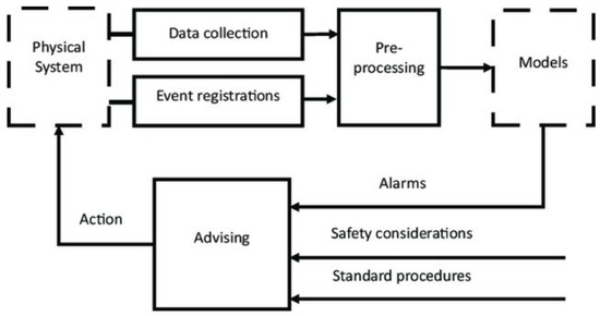
Figure 12.
High-level architecture of model-based monitoring: data collection and event logging feed pre-processing and model blocks; residuals are converted into alarms and advisories subject to safety procedures.
4.1.1. Unified Fault–Disturbance–Noise Setting
For formal analysis we adopt the standard linearized representation around the current operating point (the linearization is local but can be gain-scheduled across the torque–speed map) [117,118]:
where collects electrical and, when needed, thermal states (e.g., winding/junction lumped temperatures), are the applied voltages (or their synthesis), are measured currents/voltages/temperatures, are fault signals (open/short switch, sensor bias, phase loss, cooling failure), d are unknown but bounded disturbances (load ripple, road-induced speed oscillations), and v is measurement noise. The matrices and encode how each fault acts on state and output; their columns are the fault signatures. Electrical/thermal couplings are naturally captured by augmenting x with a reduced RC network and linearizing with respect to [119].
4.1.2. Residual Generation and Disturbance Decoupling
A residual is any signal r that is ideally zero in healthy conditions and deviates in the presence of faults. We design a stable filter that processes :
and aim at with directionally selective [120]. In the parity-space approach, let be the input–output map; any left annihilator of () produces a residual insensitive to modeling-consistent behavior. Disturbance decoupling requires , while fault detectability entails for the faults of interest. When exact decoupling is impossible (typical with torque ripple or speed oscillations), we pose a weighted design [118,121]:
with the disturbance/fault transfer matrices and the guaranteed fault-to-residual gain; standard LMI synthesis yields .
4.1.3. Observer-Based Residuals and UIO
When state estimation is available, an innovation residual is
In presence of unknown inputs d, an Unknown Input Observer (UIO) enforces , yielding exact disturbance decoupling if and satisfy the UIO existence conditions [115,117]. For thermal monitoring, augmenting (38) with RC states gives innovation residuals highly sensitive to cooling degradation (e.g., pump failure) while remaining robust to benign load variations [119].
4.1.4. Directional Residuals and Isolation
Figure 13 generalizes the architecture towards diagnosis and isolation. A normal model produces a global residual, while a bank of fault models or fault-directed filters generates directional residuals predominantly sensitive to fault [114,121]. Denoting by , we seek a signature matrix S with entries under fault in a norm (e.g., over a detection window). A well-designed bank yields a near-diagonal S, enabling isolation via .
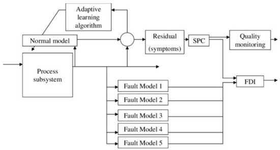
Figure 13.
Architecture for residual generation, SPC-based quality monitoring and FDI via a bank of fault models/filters. The “adaptive learning” block updates the normal model (e.g., RLS/EKF) to follow slow drifts.
4.1.5. Statistical Decision and SPC
Residuals are stochastic processes due to v and modeling errors. Under the healthy hypothesis , the innovation of a Kalman filter is Gaussian with covariance ; a generalized likelihood ratio test (GLRT) decides
with threshold chosen from a desired false-alarm probability. For incipient faults, sequential tests increase sensitivity: an EWMA chart computes and triggers when , while a CUSUM statistic detects mean shifts with minimum delay. These SPC blocks, explicit in Figure 13, form the bridge between residuals and quality monitoring/alarms [115,120].
4.1.6. Multiple-Model Bayesian Isolation
The block diagram of Figure 14 emphasizes how expert knowledge, FMEA and design-of-experiments (DOE) shape the symptom and measurement selection, producing a database used to parametrize a normal model and a set of fault models [114,121]. Let denote the hypothesis “model is true”. A recursive Bayesian isolator updates the posterior
where is the model-i prediction. Isolation follows from , while decision confidence is quantified by entropy [114,115,120].
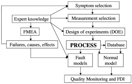
Figure 14.
Knowledge-driven workflow: symptom and measurement selection informed by expert knowledge and FMEA; DOE builds a labeled database for normal/fault models, enabling quality monitoring and FDI.
4.1.7. Adaptive Model Updating
Slow parameter drift (e.g., , , thermal conductances) is handled by the “adaptive learning algorithm” block in Figure 13. A simple and effective choice is RLS with forgetting [117,119]:
with regressor built from and parameter vector collecting the linearized entries of . The updated model keeps residuals centered under healthy operation (reducing false alarms) while preserving sensitivity to abrupt faults [119,121].
4.1.8. Thermal/Electrical Co-Monitoring
Coherent electrical–thermal monitoring improves separability of fault classes. Augment (38) with thermal states T and write the discrete RC model , where stacks copper/iron and switching losses predicted from [119]. The joint observer
produces electrical residuals (i-innovation) and thermal residuals (T mismatch). A cooling-loss fault yields large thermal residuals with small electrical innovation; an open-phase fault produces the opposite pattern. Decision logic exploits this orthogonality for isolation [119,121].
4.1.9. Set-Membership/Interval Observers
When bounds rather than statistics are available, interval observers propagate reachable sets under bounded . If a new measurement implies , a fault is declared. This deterministic approach is attractive for ISO 26262 assurance because it avoids distributional assumptions [114,122].
4.1.10. From Residuals to Actions
Finally, the “Advising” block in Figure 12 transforms decisions into derating or reconfiguration. If the posterior of an open-phase fault passes a confidence threshold, the inverter switches to two-phase operation; if thermal residuals exceed limits, the torque command is reduced according to a certified derating map. Importantly, all actions preserve the assumptions behind (38) (e.g., voltage feasibility) so that monitoring remains valid after the control reconfiguration [114,115,118,121]. In summary, the trio of Figure 12, Figure 13 and Figure 14 maps cleanly onto the formal machinery above: disturbance-decoupled residual synthesis (39) and (40), observer/UIO design for innovation-based residuals, directional banks for isolation with signature matrices, SPC/GLRT decision layers for timely alarms, Bayesian multi-model fusion informed by FMEA/DOE, and adaptive updating to track slow drift. This stack achieves high sensitivity to both abrupt electrical faults and gradual electro-thermal degradations while retaining interpretability, computational tractability, and certifiability in automotive embedded platforms [114,115,116,118,119,120,121,123].
4.2. AI/ML Models for Monitoring
Artificial-intelligence-based monitoring reframes the supervision problem in terms of statistical inference over multi-domain sequences of currents, voltages, temperatures, and vibrations [124,125]. Let a dataset be given, with the measurable outputs and the control inputs or operating conditions. The goal is to learn a parametric mapping that produces a score and a decision rule for anomaly detection, fault classification, or prognostics (RUL estimation). It is useful to distinguish between discriminative models that learn a boundary of normality, generative models that reconstruct signals or likelihoods, and sequential models that predict degradation trajectories, each with specific training objectives, computational complexity, and feasibility for real-time execution. In the case of one-class Support Vector Machines (OC-SVM) for anomaly detection, the aim is to approximate the normality manifold without fault labels [126]. The primal problem is
where are features (e.g., Park vector harmonics or STFT coefficients), controls the fraction of support vectors, and the decision function is . The dual problem is a quadratic program scaling as , but inference cost is with S support vectors; once trained, OC-SVMs run efficiently even on DSPs or MCUs. Features are typically extracted through short-time Fourier transforms or continuous wavelet transforms, providing robust time–frequency representations for fault detection. Autoencoders extend the anomaly detection paradigm by learning a latent representation and reconstructing , minimizing
with residual score indicating deviations from healthy operation. Variational autoencoders (VAE) provide probabilistic anomaly scores, enabling likelihood-based thresholding. Compact autoencoders with INT8 quantization are deployable on embedded DSPs within 10–s, while deeper VAEs are better suited for offline diagnostics [127]. Convolutional Neural Networks (CNNs) are primarily used for supervised fault classification from spectrograms or wavelet maps of current and vibration signals [128,129]. Their classification accuracy is excellent when labeled fault data are available, covering open-phase, inverter switch failures, or bearing defects. Inference is highly parallelizable on FPGAs, making CNNs attractive for real-time diagnosis provided preprocessing (FFT or CWT) is optimized. Recurrent Neural Networks (RNNs) and their gated variants (LSTM, GRU) are natural candidates for degradation modeling and RUL estimation [127]. Compact pruned variants can run online with short horizons, but full-size RNNs are typically employed offline for long-term degradation trend modeling. Transformer architectures extend this to long-range dependencies with self-attention, promising for multi-domain monitoring (electro-thermal–mechanical), but currently limited to offline analysis and digital twin frameworks due to complexity [130]. Probabilistic AI models provide explicit uncertainty quantification. Gaussian Process Regression (GPR) with kernel yields posterior mean and variance, but complexity in training limits scalability. Bayesian Neural Networks (BNN) provide posterior distributions over weights and predictive intervals, useful for certifiable safety monitoring [131], but their runtime makes them candidates for offline analysis. Overall, lightweight models such as OC-SVM, compact autoencoders, and CNNs can be integrated on DSP/FPGA controllers for online monitoring within the control loop, while more complex models (RNNs, Transformers, GPR, BNN) are reserved for offline prognostics, digital twin analyses, and cloud-based PHM frameworks, possibly distilled into simpler models for deployment [124,125]. These considerations are summarized in Table 5.
Table 5.
AI/ML models for monitoring in automotive PMSM/IPMSM drives: objectives, use, and on-board feasibility.
4.3. Hybrid Monitoring Techniques
While model-based and AI-based monitoring provide complementary strengths, the most promising strategies for safety-critical electric drives arise from their integration into hybrid approaches. The rationale is straightforward: model-based observers yield interpretable residuals derived from physics-informed equations, whereas AI models excel at detecting complex nonlinear patterns and fusing heterogeneous data. Combining the two allows the residuals to be treated not as end signals but as inputs to machine learning classifiers or regressors, thereby creating a multi-layered detection framework with enhanced robustness [132,133]. Digital twin frameworks represent a particularly relevant instantiation of this integration, enabling synchronization between physics-based reduced-order models and data-driven correctors [133,134,135]. Formally, consider the fault–disturbance–noise representation
and let be the output of a parameterized model (e.g., an observer or reduced-order thermal RC model). The residual is classically evaluated against thresholds. In a hybrid framework, instead of simple thresholding, one constructs a feature vector
where includes nonlinear embeddings such as wavelet coefficients of r, statistics over sliding windows, or projections onto parity-space residuals. This is then fed into a classifier , such as an autoencoder, CNN, or ensemble model, which maps to fault probabilities or health indices [126,129,136]. The training objective is
where ℓ is a cross-entropy or contrastive loss depending on the availability of labeled data. This architecture leverages the interpretability of physics-based residuals while exploiting the discriminative power of data-driven models [125,130]. Another powerful class of hybrid approaches relies on digital twins, where a high-fidelity physical model is continuously updated with streaming sensor data through data-driven correctors . The overall state estimate is given by
so that the state balances consistency with the physics, plausibility with the AI predictor, and fidelity with the measurements. This formulation generalizes classical Kalman filtering: the AI model effectively acts as an adaptive prior compensating for modeling errors such as saturation or temperature-dependent drift. Recent works have applied digital twins to PMSM parameter estimation [137], health status monitoring of rectifiers [138], open-circuit fault diagnosis of multilevel converters [139], and virtual thermal sensing in power electronics [140]. Broader surveys highlight their role in predictive maintenance and PHM across power electronic systems [135,141]. Physics-informed neural networks (PINNs) offer another hybrid paradigm, embedding the governing equations of the drive directly into the loss function of the network [141]. Given differential equations , one trains a neural approximation by minimizing
so that the network respects both measured data and the underlying physics. In monitoring applications, PINNs can estimate latent variables such as magnetic flux or junction temperatures, which are difficult to sense directly, while simultaneously being constrained by the machine equations. The hybrid approach also extends naturally to prognostics and health management. Model-based observers provide physics-consistent residuals and estimated parameters (e.g., winding resistance, inductance, thermal conductance). AI models then learn temporal mappings from and to health indices and RUL predictions. For instance, a recurrent network may model
with representing a normalized health state. The AI component captures nonlinear trends, while the observer guarantees that only physically meaningful variables are passed to the network, improving generalization and interpretability. Such hybrid prognostic strategies are being actively investigated for electro-thermal aging detection in automotive SiC powertrains [142] and energy consumption forecasting in sustainable transport platforms [143]. From an implementation viewpoint, hybrid monitoring balances the computational constraints of embedded systems with the flexibility of AI. Residual generation via observers or parity relations is lightweight, typically per time step. Feeding residual-based features to compact classifiers such as shallow autoencoders or kernel machines preserves online feasibility. More complex models (e.g., RNNs, Transformers) can be trained offline using residual histories and deployed in reduced distilled form for online monitoring. This division of labor between physics-based online filters and data-driven offline learners is key to achieving certifiable real-time performance under ISO 26262 constraints [144]. In summary, hybrid monitoring techniques bridge the gap between model-based interpretability and AI-based adaptability. By embedding physics in the residual generation, constraining learning with governing equations, or fusing digital twins with adaptive correctors, they deliver robust detection of both abrupt and incipient faults. Moreover, they enable prognostic estimation across electrical, thermal, and mechanical domains, all while maintaining computational feasibility for real-time automotive drives. Hybrid monitoring patterns combine physics-based residual generation with learning blocks that classify, fuse, or regularize information across domains. The most recurrent patterns can be summarized through their mathematical cores, primary monitoring objectives, and deployability on embedded automotive hardware. Residuals+ML treat physics-based residuals as features for a lightweight classifier or regressor; digital twins fuse a high-fidelity model with data-driven correctors by solving a constrained estimation problem; physics-informed neural networks (PINNs) embed the governing equations directly into the learning loss; gray-box state-space learning identifies compact parametric models regularized by physics, and safety-shielded learning projects learned decisions through certified barrier or feasibility layers to ensure invariants.
In practice, residuals+ML are the most deployable option for strict real-time budgets because residual generation is and the classifier can be kept shallow and quantized; digital twins excel when latent electro-thermal states must be estimated online with physical coherence, while heavier correctors are trained offline; PINNs and gray-box state-space models complement each other, the former enforcing equation satisfaction directly in the loss, the latter yielding compact observers with reliable innovation statistics for SPC; residuals combined with pruned RNNs provide on-board short-horizon prognostics, whereas long-horizon RUL requires offline training on fleet data; finally, safety-shielded layers and Bayesian fusion add certifiable guarantees and calibrated confidence without inflating the runtime footprint. See Table 6 for a concise summary on hybrid methods.
Table 6.
Hybrid monitoring architectures: mathematical core, objectives, and feasibility for on-board use.
4.4. Comparative Discussion: Model-Based vs. AI-Based vs. Hybrid
A principled comparison among model-based, AI-based, and hybrid monitoring can be framed in terms of (i) interpretability and reliability of the decision process, (ii) computational and memory footprint subject to real-time constraints, and (iii) integrability on automotive-grade embedded platforms. Let a monitoring pipeline output a decision based on a score and threshold . We formalize performance via a multi-criteria index
where quantifies probability calibration error (e.g., Expected Calibration Error of predicted fault probabilities), and aggregates compute latency and memory footprint under worst-case execution. Interpretability can be expressed through the existence of a physics-grounded residual map with directional sensitivity (signature matrix nearly diagonal) and a transparent decision rule (GLRT/SPC) or, in data-driven settings, through feature attributions consistent with physical invariants. Reliability is articulated as a combination of statistical risk , robustness to domain shift, and availability of formal guarantees such as disturbance decoupling or uncertainty bounds. Embedded feasibility is tied to upper bounds on inference latency , code/data size M, and determinism (bounded jitter), typically constrained by s for current loops. Model-based monitoring maximizes interpretability and affords formal guarantees via parity relations, unknown-input observers, and -optimized residuals. It offers statistical decision layers with known null distributions (e.g., for Kalman innovation), enabling precise false-alarm control. Its limitations arise under unmodeled nonlinearities and parameter drift; adaptive identification mitigates these at modest cost. AI-based monitoring excels at nonlinear pattern discovery and multi-domain fusion; probabilistic variants (GPR/BNN) provide uncertainty quantification, though often at a runtime cost incompatible with tight deadlines. Hybrid strategies inherit the interpretability of physics-based residuals and the expressivity of learned components, enabling calibrated decisions on top of meaningful features and achieving a favorable Pareto balance between accuracy, robustness, and real-time feasibility.
For a more operational view, we summarize typical computational envelopes and recommended placements. Latency ranges refer to end-to-end monitoring (residual generation + inference) and assume fixed-point or INT8 inference where applicable; memory includes model parameters and lookup structures.
To frame the alternatives, Table 7 provides a synoptic comparison of model-based, AI-based, and hybrid approaches across four axes: interpretability and guarantees, reliability and uncertainty, runtime and memory, and embedded integrability. Complementarily, Table 8 summarizes the implementation envelopes (per-step latency and memory footprint), recommended deployment roles, and certification notes, offering practical guidance for both online and offline adoption.
Table 7.
Formal comparison across interpretability/reliability and embedded feasibility.
Table 8.
Implementation envelopes and recommended deployment.
Putting the pieces together, model-based monitoring should be the backbone of the on-board layer due to interpretability, deterministic timing, and explicit guarantees; AI-based modules add sensitivity and multi-domain fusion where labeled data exist and runtime budgets allow; hybrid integration provides the best Pareto frontier by feeding physics-coherent residuals into lightweight classifiers, constraining learning with governing equations (PINN), or fusing high-fidelity twins with adaptive correctors. This stratification also supports certification: the safety case can anchor on analytical properties of the model-based core, while learned components are sandboxed, calibrated, and—when necessary—distilled and shielded by feasibility or barrier layers to maintain invariants under real-world uncertainty. To make the comparative assessment actionable, Table 9 enumerates representative faults with concrete sensor/feature choices, physics-based residuals, lightweight AI models, and decision logic suitable for embedded deployment. Each recipe is meant to be directly instantiated and tuned within the proposed monitoring stack.
Table 9.
Operational recipes for typical faults: sensors/features, residual design, AI model, decision logic, and deployment.
4.5. Battery Monitoring and Interaction with Drive Monitoring
The monitoring of the high-voltage battery cannot be considered in isolation, as its operation directly influences the performance and reliability of the entire electric drive system, and vice versa. While classical approaches treat the Battery Management System (BMS) and the Drive Monitoring System as separate layers, recent methodologies emphasize their bidirectional coupling, particularly under dynamic automotive conditions [146,147].
From a formal perspective, let the battery state vector be
where z is the state of charge (SOC), the average cell temperature, and a set of degradation indicators (e.g., internal resistance growth, capacity fade). The electric drive dynamics are characterized by the machine–inverter state vector
where are the dq-axis currents, the mechanical speed, and the semiconductor junction temperature. The coupling between the two subsystems can be expressed through the DC-link power balance:
where is the instantaneous battery power, the inverter output power towards the machine, the conversion and conduction losses, and the DC-link capacitance. Equation (46) shows that any monitoring error in the estimation of or directly propagates to the assessment of inverter stress and motor torque capability. During high-power transients, battery monitoring determines the admissible discharge power
which constrains the maximum torque reference of the drive. Conversely, monitoring of drive-side variables such as and is used to predict current ripples and thermal overloads that reflect back into higher battery RMS current and heat generation. In regenerative braking, the condition
must hold, linking the braking torque demand to the instantaneous charging capability of the cells. If this inequality is violated due to monitoring inaccuracies, the drive controller may inject currents that the battery cannot safely absorb, leading to overvoltage or lithium plating. From a monitoring design standpoint, the integration of the two domains is achieved by embedding battery state observers into the drive supervisory layer. For example, an extended state observer can be formulated as
where is the drive model, the measured drive outputs, and a coupling term updated from battery monitoring. This structure allows the drive controller to be aware of the battery’s instantaneous health state and to adapt torque commands accordingly. Conversely, the BMS incorporates drive-side residuals such as harmonic distortion in or abnormal inverter switching losses as early indicators of excessive current demand or unbalanced regenerative events [148]. In summary, battery monitoring and drive monitoring form a coupled system where the accuracy of one directly impacts the reliability of the other. By enforcing power balance constraints (46), saturation limits on and , and by cross-feeding residuals between observers, it is possible to design a unified monitoring layer. This co-design approach enhances safety (avoiding overcurrent or overvoltage), improves efficiency (optimizing energy recovery in regenerative braking), and extends lifetime (reducing thermal and electrochemical stress), thus aligning monitoring strategies with both functional safety and sustainability objectives in automotive electric drives [149,150].
5. Concluding Remarks and Future Trends
This review has analyzed the state of the art in modeling, control, and monitoring of automotive power drive systems, showing that while each of these domains has reached a high level of maturity individually, their integration remains limited. Existing techniques for multiphysics modeling provide accurate representations of electromagnetic and thermal behavior, yet are seldom exploited beyond the design phase. Control strategies range from mature field-oriented and direct torque control to advanced predictive and adaptive schemes, but monitoring considerations are rarely embedded into their formulation. Likewise, monitoring frameworks are rich in methods—spanning signal-based, model-based, and AI-based approaches—yet they typically operate in parallel to control rather than as part of a unified architecture. This fragmentation highlights both the progress achieved and the limitations that still need to be overcome. In addition, the analysis underlined how energy storage systems and their monitoring strongly influence drive performance and sustainability. Different battery chemistries exhibit diverse capabilities in terms of energy density, power acceptance, and regenerative braking, with direct impact on efficiency and environmental footprint. Bidirectional converters further enable controlled energy flow between storage and drive, making their modeling and monitoring essential for safe and efficient integration. Looking forward, several trends are expected to shape the evolution of electric drive systems:
- Model–control–monitoring integration. Physics-based models will increasingly be shared across design, control, and monitoring layers to ensure consistency and certification traceability.
- Hybrid and physics-informed AI. Data-driven methods will be combined with physics-based models to achieve adaptability with interpretability and safety guarantees.
- Constraint-aware and multi-domain control. Controllers such as MPC and RL will embed electro-thermal and NVH objectives, with design methodologies becoming more systematic.
- Battery–drive co-monitoring. Joint supervision of SOC, SOH, SOP and drive-side variables will ensure safe charging/discharging, optimize regenerative braking, and extend lifetime.
- Scalable prognostics and fleet learning. Fleet-level data will train degradation and RUL models, with lightweight on-board implementations for real-time monitoring.
- Functional safety and certification. ISO 26262 compliance will require hybrid schemes combining formal guarantees with AI under safety envelopes.
- Real-time feasibility. Wide-bandgap devices and higher switching frequencies will push towards domain-specific accelerators for microsecond-level control and monitoring.
In conclusion, the future of automotive electric drives lies in unified architectures where modeling, control, and monitoring operate together rather than in isolation. Achieving this integration is essential to deliver systems that are efficient, robust, certifiable, and sustainable, supporting the large-scale transition to electrified mobility.
Key Takeaways
- Integration of modeling, control, and monitoring is the decisive step beyond fragmented approaches.
- Battery technologies, bidirectional converters, and regenerative braking must be jointly considered with drive control.
- Intelligent and hybrid controllers complement classical strategies, offering adaptability under safety constraints.
- Robust monitoring and prognostics are central to reliability, lifetime extension, and sustainability.
Author Contributions
Conceptualization, P.D.; Methodology, P.D., S.S., S.C. and O.H.; Investigation, P.D., S.S., S.C. and O.H.; Writing—original draft, P.D.; Writing—review and editing, P.D., S.S., S.C. and O.H.; Visualization, P.D. and S.C.; Supervision, S.S. and O.H.; Project administration, S.S. All authors have read and agreed to the published version of the manuscript.
Funding
This work was supported in part by the European Union’s Horizon 2020 research and innovation program under the HIEFFICIENT project (Grant Agreement No. 769429); in part by the Italian National Recovery and Resilience Plan (PNRR) under CN1 “HPC, Big data e Quantum Computing”—Spoke 6 “Multiscale modeling engineering applications”; and in part by the Italian Ministry of University and Research (MUR) under the initiative FORELab—Future ORiented Engineering Laboratory.
Data Availability Statement
No new data were generated or analyzed in this study. All information presented is based on previously published sources, which are appropriately cited throughout the manuscript.
Conflicts of Interest
Author Sajib Chakraborty and Omar Hegazy were employed by the company Flanders Make. The remaining authors declare that the research was conducted in the absence of any commercial or financial relationships that could be construed as a potential conflict of interest.
References
- ISO 26262; Road Vehicles—Functional Safety. International Organization for Standardization: Geneva, Switzerland, 2018.
- Kumar, R.R.; Andriollo, M.; Cirrincione, G.; Cirrincione, M.; Tortella, A. A comprehensive review of conventional and intelligence-based approaches for the fault diagnosis and condition monitoring of induction motors. Energies 2022, 15, 8938. [Google Scholar] [CrossRef]
- Sardar, M.U.; Vaimann, T.; Kütt, L.; Kallaste, A.; Asad, B.; Akbar, S.; Kudelina, K. Inverter-fed motor drive system: A systematic analysis of condition monitoring and practical diagnostic techniques. Energies 2023, 16, 5628. [Google Scholar] [CrossRef]
- Mercorelli, P. Control of permanent magnet synchronous motors for track applications. Electronics 2023, 12, 3285. [Google Scholar] [CrossRef]
- Gultekin, M.A.; Bazzi, A. Review of fault detection and diagnosis techniques for AC motor drives. Energies 2023, 16, 5602. [Google Scholar] [CrossRef]
- Chen, Z.; Liu, J. Exploring the Drive Motor of Electric Vehicles: Structure, Temperature Rises, and Operational Control of Permanent Magnet Motors. World Electr. Veh. J. 2024, 15, 483. [Google Scholar] [CrossRef]
- Sergakis, A.; Salinas, M.; Gkiolekas, N.; Gyftakis, K.N. A Review of Condition Monitoring of Permanent Magnet Synchronous Machines: Techniques, Challenges and Future Directions. Energies 2025, 18, 1177. [Google Scholar] [CrossRef]
- Sangeetha, E.; Ramachandran, V. Different topologies of electrical machines, storage systems, and power electronic converters and their control for battery electric vehicles—A technical review. Energies 2022, 15, 8959. [Google Scholar] [CrossRef]
- Jiang, Y.; Ji, B.; Zhang, J.; Yan, J.; Li, W. An overview of diagnosis methods of stator winding inter-turn short faults in permanent-magnet synchronous motors for electric vehicles. World Electr. Veh. J. 2024, 15, 165. [Google Scholar] [CrossRef]
- Umland, N.; Winkler, K.; Inkermann, D. Multidisciplinary design automation of electric motors—Systematic literature review and methodological framework. Energies 2023, 16, 7070. [Google Scholar] [CrossRef]
- Gundabattini, E.; Mystkowski, A.; Idzkowski, A.; R, R.S.; Solomon, D.G. Thermal mapping of a high-speed electric motor used for traction applications and analysis of various cooling methods—A review. Energies 2021, 14, 1472. [Google Scholar] [CrossRef]
- Ullah, K.; Guzinski, J.; Mirza, A.F. Critical review on robust speed control techniques for permanent magnet synchronous motor (PMSM) speed regulation. Energies 2022, 15, 1235. [Google Scholar] [CrossRef]
- El Hadraoui, H.; Zegrari, M.; Chebak, A.; Laayati, O.; Guennouni, N. A multi-criteria analysis and trends of electric motors for electric vehicles. World Electr. Veh. J. 2022, 13, 65. [Google Scholar] [CrossRef]
- Aiso, K.; Akatsu, K. Performance comparison of high-speed motors for electric vehicle. World Electr. Veh. J. 2022, 13, 57. [Google Scholar] [CrossRef]
- Shen, Q.; Zhou, Z.; Li, S.; Liao, X.; Wang, T.; He, X.; Zhang, J. Design and analysis of the high-speed permanent magnet motors: A review on the state of the art. Machines 2022, 10, 549. [Google Scholar] [CrossRef]
- Stumpf, P.; Tóth-Katona, T. Recent achievements in the control of interior permanent-magnet synchronous machine drives: A comprehensive overview of the state of the art. Energies 2023, 16, 5103. [Google Scholar] [CrossRef]
- Meddour, A.R.; Rizoug, N.; Leserf, P.; Vagg, C.; Burke, R.; Larouci, C. Optimization of the Lifetime and Cost of a PMSM in an Electric Vehicle Drive Train. Energies 2023, 16, 5200. [Google Scholar] [CrossRef]
- Kinoti, E.; Mosetlhe, T.C.; Yusuff, A.A. Multi-Criteria Analysis of Electric Vehicle Motor Technologies: A Review. World Electr. Veh. J. 2024, 15, 541. [Google Scholar] [CrossRef]
- Khaneghah, M.Z.; Alzayed, M.; Chaoui, H. Fault detection and diagnosis of the electric motor drive and battery system of electric vehicles. Machines 2023, 11, 713. [Google Scholar] [CrossRef]
- Vlachou, V.I.; Sakkas, G.K.; Xintaropoulos, F.P.; Pechlivanidou, M.S.C.; Kefalas, T.D.; Tsili, M.A.; Kladas, A.G. Overview on permanent magnet motor trends and developments. Energies 2024, 17, 538. [Google Scholar] [CrossRef]
- Al Sakka, M.; Geury, T.; El Baghdadi, M.; Dhaens, M.; Al Sakka, M.; Hegazy, O. Review of fault tolerant multi-motor drive topologies for automotive applications. Energies 2022, 15, 5529. [Google Scholar] [CrossRef]
- Mazali, I.I.; Daud, Z.H.C.; Hamid, M.K.A.; Tan, V.; Samin, P.M.; Jubair, A.; Ibrahim, K.A.; Kob, M.S.C.; Xinrui, W.; Talib, M.H.A. Review of the methods to optimize power flow in electric vehicle powertrains for efficiency and driving performance. Appl. Sci. 2022, 12, 1735. [Google Scholar] [CrossRef]
- Frikha, M.A.; Croonen, J.; Deepak, K.; Benômar, Y.; El Baghdadi, M.; Hegazy, O. Multiphase Motors and Drive Systems for Electric Vehicle Powertrains: State of the Art Analysis and Future Trends. Energies 2023, 16, 768. [Google Scholar] [CrossRef]
- Kakouche, K.; Oubelaid, A.; Mezani, S.; Rekioua, D.; Rekioua, T. Different Control Techniques of Permanent Magnet Synchronous Motor with Fuzzy Logic for Electric Vehicles: Analysis, Modelling, and Comparison. Energies 2023, 16, 3116. [Google Scholar] [CrossRef]
- Gonzalez-Abreu, A.D.; Osornio-Rios, R.A.; Jaen-Cuellar, A.Y.; Delgado-Prieto, M.; Antonino-Daviu, J.A.; Karlis, A. Advances in Power Quality Analysis Techniques for Electrical Machines and Drives: A Review. Energies 2022, 15, 1909. [Google Scholar] [CrossRef]
- Rimpas, D.; Kaminaris, S.D.; Piromalis, D.D.; Vokas, G.; Arvanitis, K.G.; Karavas, C.S. Comparative Review of Motor Technologies for Electric Vehicles Powered by a Hybrid Energy Storage System Based on Multi-Criteria Analysis. Energies 2023, 16, 2555. [Google Scholar] [CrossRef]
- Ibrahim, M.; Rassõlkin, A.; Vaimann, T.; Kallaste, A. Overview on digital twin for autonomous electrical vehicles propulsion drive system. Sustainability 2022, 14, 601. [Google Scholar] [CrossRef]
- Idoko, H.C.; Akuru, U.B.; Wang, R.J.; Popoola, O. Potentials of brushless stator-mounted machines in electric vehicle drives—A literature review. World Electr. Veh. J. 2022, 13, 93. [Google Scholar] [CrossRef]
- Lan, Y.; Benomar, Y.; Deepak, K.; Aksoz, A.; Baghdadi, M.E.; Bostanci, E.; Hegazy, O. Switched reluctance motors and drive systems for electric vehicle powertrains: State of the art analysis and future trends. Energies 2021, 14, 2079. [Google Scholar] [CrossRef]
- Deepak, K.; Frikha, M.A.; Benômar, Y.; El Baghdadi, M.; Hegazy, O. In-wheel motor drive systems for electric vehicles: State of the art, challenges, and future trends. Energies 2023, 16, 3121. [Google Scholar] [CrossRef]
- Ibrahim, M.; Järg, O.; Seppago, R.; Rassõlkin, A. Performance Optimization of a High-Speed Permanent Magnet Synchronous Motor Drive System for Formula Electric Vehicle Application. Sensors 2025, 25, 3156. [Google Scholar] [CrossRef]
- Linse, C.; Kuhn, R. 10—Design of high-voltage battery packs for electric vehicles. In Advances in Battery Technologies for Electric Vehicles; Scrosati, B., Garche, J., Tillmetz, W., Eds.; Woodhead Publishing Series in Energy; Woodhead Publishing: Cambridge, UK, 2015; pp. 245–263. [Google Scholar] [CrossRef]
- Hauser, A.; Kuhn, R. 11—High-voltage battery management systems (BMS) for electric vehicles. In Advances in Battery Technologies for Electric Vehicles; Scrosati, B., Garche, J., Tillmetz, W., Eds.; Woodhead Publishing Series in Energy; Woodhead Publishing: Cambridge, UK, 2015; pp. 265–282. [Google Scholar] [CrossRef]
- Gabbar, H.A.; Othman, A.M.; Abdussami, M.R. Review of Battery Management Systems (BMS) Development and Industrial Standards. Technologies 2021, 9, 28. [Google Scholar] [CrossRef]
- Habib, A.K.M.A.; Hasan, M.K.; Issa, G.F.; Singh, D.; Islam, S.; Ghazal, T.M. Lithium-Ion Battery Management System for Electric Vehicles: Constraints, Challenges, and Recommendations. Batteries 2023, 9, 152. [Google Scholar] [CrossRef]
- Krishna, T.N.V.; Kumar, S.V.S.V.P.D.; Srinivasa Rao, S.; Chang, L. Powering the Future: Advanced Battery Management Systems (BMS) for Electric Vehicles. Energies 2024, 17, 3360. [Google Scholar] [CrossRef]
- Karmakar, S.; Bohre, A.K.; Bera, T.K. Recent Advancements in Cell Balancing Techniques of BMS for EVs: A Critical Review. IEEE Trans. Ind. Appl. 2025, 61, 3468–3484. [Google Scholar] [CrossRef]
- Popp, A.; Fechtner, H.; Schmuelling, B.; Kremzow-Tennie, S.; Scholz, T.; Pautzke, F. Battery Management Systems Topologies: Applications: Implications of different voltage levels. In Proceedings of the 2021 IEEE 4th International Conference on Power and Energy Applications (ICPEA), Busan, Republic of Korea, 9–11 October 2021; pp. 43–50. [Google Scholar] [CrossRef]
- Qin, H.; Kimball, J.W. Generalized Average Modeling of Dual Active Bridge DC–DC Converter. IEEE Trans. Power Electron. 2012, 27, 2078–2084. [Google Scholar] [CrossRef]
- Mueller, J.A.; Kimball, J.W. Modeling Dual Active Bridge Converters in DC Distribution Systems. IEEE Trans. Power Electron. 2019, 34, 5867–5879. [Google Scholar] [CrossRef]
- Rolak, M.; Twardy, M.; Soból, C. Generalized Average Modeling of a Dual Active Bridge DC-DC Converter with Triple-Phase-Shift Modulation. Energies 2022, 15, 6092. [Google Scholar] [CrossRef]
- Ghosh, S.; Das, D.; Singh, B.; Janardhanan, S.; Mishra, S. Frequency-Domain Modeling of Dual-Active-Bridge Converter Based on Harmonic Balance Approach. IEEE J. Emerg. Sel. Top. Ind. Electron. 2022, 3, 166–176. [Google Scholar] [CrossRef]
- Singh, A.; Yadav, A.K.; Khaligh, A. Steady-State Modeling of a Dual-Active Bridge AC–DC Converter Considering Circuit Nonidealities and Intracycle Transient Effects. IEEE Trans. Power Electron. 2021, 36, 11276–11287. [Google Scholar] [CrossRef]
- Mou, D.; Yuan, L.; Li, J.; Hou, N.; Li, J.; Li, Y.; Zhao, Z. Modeling and Analysis of Hybrid Dual Active Bridge Converter to Optimize Efficiency Over Whole Operating Range. IEEE J. Emerg. Sel. Top. Power Electron. 2023, 11, 432–441. [Google Scholar] [CrossRef]
- Li, L.; Xu, G.; Sha, D.; Liu, Y.; Sun, Y.; Su, M. Review of Dual-Active-Bridge Converters With Topological Modifications. IEEE Trans. Power Electron. 2023, 38, 9046–9076. [Google Scholar] [CrossRef]
- Shao, S.; Chen, L.; Shan, Z.; Gao, F.; Chen, H.; Sha, D.; Dragičević, T. Modeling and Advanced Control of Dual-Active-Bridge DC–DC Converters: A Review. IEEE Trans. Power Electron. 2022, 37, 1524–1547. [Google Scholar] [CrossRef]
- Li, X.; Pou, J.; Dong, J.; Lin, F.; Wen, C.; Mukherjee, S.; Zhang, X. Data-Driven Modeling With Experimental Augmentation for the Modulation Strategy of the Dual-Active-Bridge Converter. IEEE Trans. Ind. Electron. 2024, 71, 2626–2637. [Google Scholar] [CrossRef]
- Poorfakhraei, A.; Narimani, M.; Emadi, A. A Review of Modulation and Control Techniques for Multilevel Inverters in Traction Applications. IEEE Access 2021, 9, 24187–24204. [Google Scholar] [CrossRef]
- Jayakumar, V.; Chokkalingam, B.; Munda, J.L. A Comprehensive Review on Space Vector Modulation Techniques for Neutral Point Clamped Multi-Level Inverters. IEEE Access 2021, 9, 112104–112144. [Google Scholar] [CrossRef]
- Jin, X.; Li, S.; Sun, W.; Chen, W.; Gu, X.; Zhang, G. Optimized Synchronous SPWM Modulation Strategy for Traction Inverters Based on Non-Equally Spaced Carriers. World Electr. Veh. J. 2023, 14, 157. [Google Scholar] [CrossRef]
- Taha, W.; Azer, P.; Callegaro, A.D.; Emadi, A. Multiphase Traction Inverters: State-of-the-Art Review and Future Trends. IEEE Access 2022, 10, 4580–4599. [Google Scholar] [CrossRef]
- Jelodar, Y.J.; Salari, O.; Youssef, M.Z.; Ebrahimi, J.; Bakhshai, A. A Novel Control Scheme for Traction Inverters in Electric Vehicles With an Optimal Efficiency Across the Entire Speed Range. IEEE Access 2024, 12, 25906–25916. [Google Scholar] [CrossRef]
- Fedele, E.; Cervone, A.; Spina, I.; Iannuzzi, D.; Pizzo, A.D. Multiobjective Vector Modulation for Improved Control of NPC-Based Multi-Source Inverters in Hybrid Traction Systems. IEEE J. Emerg. Sel. Top. Power Electron. 2022, 10, 7464–7474. [Google Scholar] [CrossRef]
- Lee, J.G.; Lim, D.K. A Stepwise Optimal Design Applied to an Interior Permanent Magnet Synchronous Motor for Electric Vehicle Traction Applications. IEEE Access 2021, 9, 115090–115099. [Google Scholar] [CrossRef]
- Hussain, A.; Baig, Z.; Toor, W.T.; Ali, U.; Idrees, M.; Shloul, T.A.; Ghadi, Y.Y.; Alkahtani, H.K. Wound Rotor Synchronous Motor as Promising Solution for Traction Applications. Electronics 2022, 11, 4116. [Google Scholar] [CrossRef]
- Kumar, A.; Chandekar, A.; Deshmukh, P.; Ugale, R. Development of electric vehicle with permanent magnet synchronous motor and its analysis with drive cycles in MATLAB/Simulink. Mater. Today Proc. 2023, 72, 643–651. [Google Scholar] [CrossRef]
- Dmitrievskii, V.; Prakht, V.; Anuchin, A.; Kazakbaev, V. Design Optimization of a Traction Synchronous Homopolar Motor. Mathematics 2021, 9, 1352. [Google Scholar] [CrossRef]
- Gierczynski, M.; Grzesiak, L.M. Comparative Analysis of the Steady-State Model Including Non-Linear Flux Linkage Surfaces and the Simplified Linearized Model when Applied to a Highly-Saturated Permanent Magnet Synchronous Machine—Evaluation Based on the Example of the BMW i3 Traction Motor. Energies 2021, 14, 2343. [Google Scholar] [CrossRef]
- Ortega, A.J.P.; Das, S.; Islam, R.; Kouhshahi, M.B. High-Fidelity Analysis With Multiphysics Simulation for Performance Evaluation of Electric Motors Used in Traction Applications. IEEE Trans. Ind. Appl. 2023, 59, 1273–1282. [Google Scholar] [CrossRef]
- Fang, X.; Lin, S.; Wang, X.; Yang, Z.; Lin, F.; Tian, Z. Model Predictive Current Control of Traction Permanent Magnet Synchronous Motors in Six-Step Operation for Railway Application. IEEE Trans. Ind. Electron. 2022, 69, 8751–8759. [Google Scholar] [CrossRef]
- Dini, P.; Saponara, S. Model-based design of an improved electric drive controller for high-precision applications based on feedback linearization technique. Electronics 2021, 10, 2954. [Google Scholar] [CrossRef]
- Zhao, Y.; Yu, H.; Wang, S. Development of Optimized Cooperative Control Based on Feedback Linearization and Error Port-Controlled Hamiltonian for Permanent Magnet Synchronous Motor. IEEE Access 2021, 9, 141036–141047. [Google Scholar] [CrossRef]
- Accetta, A.; Cirrincione, M.; Pucci, M.; Sferlazza, A. Feedback Linearization Based Nonlinear Control of SynRM Drives Accounting for Self- and Cross-Saturation. IEEE Trans. Ind. Appl. 2022, 58, 3637–3651. [Google Scholar] [CrossRef]
- Accetta, A.; Cirrincione, M.; D’Ippolito, F.; Pucci, M.; Sferlazza, A. Adaptive Feedback Linearization Control of SynRM Drives With On-Line Inductance Estimation. IEEE Trans. Ind. Appl. 2023, 59, 1824–1835. [Google Scholar] [CrossRef]
- Bernardeschi, C.; Dini, P.; Domenici, A.; Palmieri, M.; Saponara, S. Formal verification and co-simulation in the design of a synchronous motor control algorithm. Energies 2020, 13, 4057. [Google Scholar] [CrossRef]
- Pacini, F.; Di Matteo, S.; Dini, P.; Fanucci, L.; Bucchi, F. Innovative Plug-and-Play System for Electrification of Wheel-Chairs. IEEE Access 2023, 11, 89038–89051. [Google Scholar] [CrossRef]
- Dini, P.; Saponara, S. Review on model based design of advanced control algorithms for cogging torque reduction in power drive systems. Energies 2022, 15, 8990. [Google Scholar] [CrossRef]
- Dini, P.; Saponara, S. Cogging torque reduction in brushless motors by a nonlinear control technique. Energies 2019, 12, 2224. [Google Scholar] [CrossRef]
- Bernardeschi, C.; Dini, P.; Domenici, A.; Mouhagir, A.; Palmieri, M.; Saponara, S.; Sassolas, T.; Zaourar, L. Co-simulation of a model predictive control system for automotive applications. In Proceedings of the International Conference on Software Engineering and Formal Methods, Virtual, 6–10 December 2021; Springer: Berlin/Heidelberg, Germany, 2021; pp. 204–220. [Google Scholar]
- Dini, P.; Saponara, S. Processor-in-the-Loop Validation of a Gradient Descent-Based Model Predictive Control for Assisted Driving and Obstacles Avoidance Applications. IEEE Access 2022, 10, 67958–67975. [Google Scholar] [CrossRef]
- Rodriguez, J.; Garcia, C.; Mora, A.; Davari, S.A.; Rodas, J.; Valencia, D.F.; Elmorshedy, M.; Wang, F.; Zuo, K.; Tarisciotti, L.; et al. Latest Advances of Model Predictive Control in Electrical Drives—Part II: Applications and Benchmarking With Classical Control Methods. IEEE Trans. Power Electron. 2022, 37, 5047–5061. [Google Scholar] [CrossRef]
- Hang, P.; Xia, X.; Chen, G.; Chen, X. Active Safety Control of Automated Electric Vehicles at Driving Limits: A Tube-Based MPC Approach. IEEE Trans. Transp. Electrif. 2022, 8, 1338–1349. [Google Scholar] [CrossRef]
- Çavuş, B.; Aktaş, M. MPC-Based Flux Weakening Control for Induction Motor Drive With DTC for Electric Vehicles. IEEE Trans. Power Electron. 2023, 38, 4430–4439. [Google Scholar] [CrossRef]
- Xue, Z.; Niu, S.; Chau, A.M.H.; Luo, Y.; Lin, H.; Li, X. Recent advances in multi-phase electric drives model predictive control in renewable energy application: A state-of-the-art review. World Electr. Veh. J. 2023, 14, 44. [Google Scholar] [CrossRef]
- Dini, P.; Ariaudo, G.; Botto, G.; Greca, F.L.; Saponara, S. Real-time electro-thermal modelling and predictive control design of resonant power converter in full electric vehicle applications. IET Power Electron. 2023, 16, 2045–2064. [Google Scholar] [CrossRef]
- Dini, P.; Basso, G.; Saponara, S.; Chakraborty, S.; Hegazy, O. Real-Time AMPC for Loss Reduction in 48 V Six-Phase Synchronous Motor Drives. IET Power Electron. 2025, 18, e70072. [Google Scholar] [CrossRef]
- Wu, L.; Liu, J.; Vazquez, S.; Mazumder, S.K. Sliding Mode Control in Power Converters and Drives: A Review. IEEE/CAA J. Autom. Sin. 2022, 9, 392–406. [Google Scholar] [CrossRef]
- Li, K.; Ding, J.; Sun, X.; Tian, X. Overview of Sliding Mode Control Technology for Permanent Magnet Synchronous Motor System. IEEE Access 2024, 12, 71685–71704. [Google Scholar] [CrossRef]
- V, K.; Rai, R.; Singh, B. Sliding Model-Based Predictive Torque Control of Induction Motor for Electric Vehicle. IEEE Trans. Ind. Appl. 2022, 58, 742–752. [Google Scholar] [CrossRef]
- Hou, L.; Ma, J.; Wang, W. Sliding Mode Predictive Current Control of Permanent Magnet Synchronous Motor With Cascaded Variable Rate Sliding Mode Speed Controller. IEEE Access 2022, 10, 33992–34002. [Google Scholar] [CrossRef]
- Wang, S.; Wang, H.; Tang, C.; Li, J.; Liang, D.; Qu, Y. Research on Control Strategy of Permanent Magnet Synchronous Motor Based on Fast Terminal Super-Twisting Sliding Mode Observer. IEEE Access 2024, 12, 141905–141915. [Google Scholar] [CrossRef]
- Ding, H.; Zou, X.; Li, J. Sensorless Control Strategy of Permanent Magnet Synchronous Motor Based on Fuzzy Sliding Mode Observer. IEEE Access 2022, 10, 36743–36752. [Google Scholar] [CrossRef]
- Zuo, Y.; Lai, C.; Iyer, K.L.V. A Review of Sliding Mode Observer Based Sensorless Control Methods for PMSM Drive. IEEE Trans. Power Electron. 2023, 38, 11352–11367. [Google Scholar] [CrossRef]
- Tahami, H.; Saberi, S.; Ali, B.M.; AbdulAmeer, S.; Abdul Hussein, A.H.; Chaoui, H. A robust hinf-based state feedback control of permanent magnet synchronous motor drives using adaptive fuzzy sliding mode observers. Actuators 2024, 13, 307. [Google Scholar] [CrossRef]
- Wang, R.; Sun, Q.; Sun, C.; Zhang, H.; Gui, Y.; Wang, P. Vehicle-Vehicle Energy Interaction Converter of Electric Vehicles: A Disturbance Observer Based Sliding Mode Control Algorithm. IEEE Trans. Veh. Technol. 2021, 70, 9910–9921. [Google Scholar] [CrossRef]
- Dini, P.; Saponara, S. Design of adaptive controller exploiting learning concepts applied to a BLDC-based drive system. Energies 2020, 13, 2512. [Google Scholar] [CrossRef]
- Kamiński, M.; Szabat, K. Adaptive control structure with neural data processing applied for electrical drive with elastic shaft. Energies 2021, 14, 3389. [Google Scholar] [CrossRef]
- Liu, Y.; Zhang, Y.; Yu, H.; Nie, Z.; Liu, Y.; Chen, Z. A novel data-driven controller for plug-in hybrid electric vehicles with improved adaptabilities to driving environment. J. Clean. Prod. 2022, 334, 130250. [Google Scholar] [CrossRef]
- Carlet, P.G.; Favato, A.; Bolognani, S.; Dörfler, F. Data-Driven Continuous-Set Predictive Current Control for Synchronous Motor Drives. IEEE Trans. Power Electron. 2022, 37, 6637–6646. [Google Scholar] [CrossRef]
- Wei, Y.; Young, H.; Wang, F.; Rodríguez, J. Generalized Data-Driven Model-Free Predictive Control for Electrical Drive Systems. IEEE Trans. Ind. Electron. 2023, 70, 7642–7652. [Google Scholar] [CrossRef]
- Wu, W.; Qiu, L.; Liu, X.; Guo, F.; Rodriguez, J.; Ma, J.; Fang, Y. Data-Driven Iterative Learning Predictive Control for Power Converters. IEEE Trans. Power Electron. 2022, 37, 14028–14033. [Google Scholar] [CrossRef]
- Wu, W.; Qiu, L.; Rodriguez, J.; Liu, X.; Ma, J.; Fang, Y. Data-Driven Finite Control-Set Model Predictive Control for Modular Multilevel Converter. IEEE J. Emerg. Sel. Top. Power Electron. 2023, 11, 523–531. [Google Scholar] [CrossRef]
- Cheng, M.; Zhao, X.; Dhimish, M.; Qiu, W.; Niu, S. A Review of Data-Driven Surrogate Models for Design Optimization of Electric Motors. IEEE Trans. Transp. Electrif. 2024, 10, 8413–8431. [Google Scholar] [CrossRef]
- Song, Z.; Yang, J.; Mei, X.; Tao, T.; Xu, M. Deep reinforcement learning for permanent magnet synchronous motor speed control systems. Neural Comput. Appl. 2021, 33, 5409–5418. [Google Scholar] [CrossRef]
- Nicola, M.; Nicola, C.I.; Selișteanu, D. Improvement of PMSM sensorless control based on synergetic and sliding mode controllers using a reinforcement learning deep deterministic policy gradient agent. Energies 2022, 15, 2208. [Google Scholar] [CrossRef]
- Zhao, J.; Yang, C.; Gao, W.; Zhou, L. Reinforcement Learning and Optimal Control of PMSM Speed Servo System. IEEE Trans. Ind. Electron. 2023, 70, 8305–8313. [Google Scholar] [CrossRef]
- Schenke, M.; Wallscheid, O. A Deep Q-Learning Direct Torque Controller for Permanent Magnet Synchronous Motors. IEEE Open J. Ind. Electron. Soc. 2021, 2, 388–400. [Google Scholar] [CrossRef]
- Book, G.; Traue, A.; Balakrishna, P.; Brosch, A.; Schenke, M.; Hanke, S.; Kirchgässner, W.; Wallscheid, O. Transferring Online Reinforcement Learning for Electric Motor Control From Simulation to Real-World Experiments. IEEE Open J. Power Electron. 2021, 2, 187–201. [Google Scholar] [CrossRef]
- Wang, Y.; Fang, S.; Hu, J.; Huang, D. A Novel Active Disturbance Rejection Control of PMSM Based on Deep Reinforcement Learning for More Electric Aircraft. IEEE Trans. Energy Convers. 2023, 38, 1461–1470. [Google Scholar] [CrossRef]
- Wang, Y.; Fang, S.; Hu, J. Active Disturbance Rejection Control Based on Deep Reinforcement Learning of PMSM for More Electric Aircraft. IEEE Trans. Power Electron. 2023, 38, 406–416. [Google Scholar] [CrossRef]
- Kiliç, E. Deep Reinforcement Learning-Based Controller for Field-Oriented Control of SynRM. IEEE Access 2025, 13, 2855–2861. [Google Scholar] [CrossRef]
- Li, S.; Won, H.; Fu, X.; Fairbank, M.; Wunsch, D.C.; Alonso, E. Neural-Network Vector Controller for Permanent-Magnet Synchronous Motor Drives: Simulated and Hardware-Validated Results. IEEE Trans. Cybern. 2020, 50, 3218–3230. [Google Scholar] [CrossRef]
- Fatemimoghadam, A.; Varaha Iyer, L.; Kar, N.C. Real-Time Validation of Enhanced Permanent Magnet Synchronous Motor Drive Using Dense-Neural-Network-Based Control. IEEE Access 2024, 12, 73323–73339. [Google Scholar] [CrossRef]
- Mohan, H.; Agrawal, G.; Jately, V.; Sharma, A.; Azzopardi, B. Neural network-driven sensorless speed control of EV drive using PMSM. Mathematics 2023, 11, 4029. [Google Scholar] [CrossRef]
- Pang, S.; Zhang, Y.; Huangfu, Y.; Li, X.; Tan, B.; Li, P.; Tian, C.; Quan, S. A Virtual MPC-Based Artificial Neural Network Controller for PMSM Drives in Aircraft Electric Propulsion System. IEEE Trans. Ind. Appl. 2024, 60, 3603–3612. [Google Scholar] [CrossRef]
- Skowron, M.; Orlowska-Kowalska, T.; Kowalski, C.T. Detection of Permanent Magnet Damage of PMSM Drive Based on Direct Analysis of the Stator Phase Currents Using Convolutional Neural Network. IEEE Trans. Ind. Electron. 2022, 69, 13665–13675. [Google Scholar] [CrossRef]
- Liu, Z.H.; Nie, J.; Wei, H.L.; Chen, L.; Li, X.H.; Lv, M.Y. Switched PI Control Based MRAS for Sensorless Control of PMSM Drives Using Fuzzy-Logic-Controller. IEEE Open J. Power Electron. 2022, 3, 368–381. [Google Scholar] [CrossRef]
- Suganthi, S.; Karpagam, R. Dynamic performance improvement of PMSM drive using fuzzy-based adaptive control strategy for EV applications. J. Power Electron. 2023, 23, 510–521. [Google Scholar] [CrossRef]
- Bouguenna, I.F.; Tahour, A.; Kennel, R.; Abdelrahem, M. Multiple-vector model predictive control with fuzzy logic for PMSM electric drive systems. Energies 2021, 14, 1727. [Google Scholar] [CrossRef]
- Belkhier, Y.; Oubelaid, A.; Shaw, R.N. Hybrid power management and control of fuel cells-battery energy storage system in hybrid electric vehicle under three different modes. Energy Storage 2024, 6, e511. [Google Scholar] [CrossRef]
- Ishwarya, U.; Srimathi, R.; Nithishkumar, K.; Vijaya Chandrakala, K.; Saravanan, S.; Arun Shankar, V. Optimum Speed Control of Permanent Magnet Synchronous Motor using Artificial Neural Network-Based Field-Oriented Controller. In Proceedings of the 2024 3rd International Conference on Artificial Intelligence For Internet of Things (AIIoT), Vellore, India, 3–4 May 2024; pp. 1–6. [Google Scholar] [CrossRef]
- Zhang, X.; Zhang, H.; Yan, K. Hybrid Vector Model Predictive Control for Open-Winding PMSM Drives. IEEE Trans. Transp. Electrif. 2024, 10, 4322–4333. [Google Scholar] [CrossRef]
- Khanh, P.Q.; Anh, H.P.H. Hybrid optimal fuzzy Jaya technique for advanced PMSM driving control. Electr. Eng. 2023, 105, 3629–3646. [Google Scholar] [CrossRef]
- Orlowska-Kowalska, T.; Wolkiewicz, M.; Pietrzak, P.; Skowron, M.; Ewert, P.; Tarchala, G.; Krzysztofiak, M.; Kowalski, C.T. Fault Diagnosis and Fault-Tolerant Control of PMSM Drives–State of the Art and Future Challenges. IEEE Access 2022, 10, 59979–60024. [Google Scholar] [CrossRef]
- Attaianese, C.; D’Arpino, M.; Monaco, M.D.; Noia, L.P.D. Model-Based Detection and Estimation of DC Offset of Phase Current Sensors for Field Oriented PMSM Drives. IEEE Trans. Ind. Electron. 2023, 70, 6316–6325. [Google Scholar] [CrossRef]
- Attaianese, C.; D’Arpino, M.; Monaco, M.D.; Noia, L.P.D. Current Signature Modeling of Surface-Mounted PMSM Drives With Current Sensors Faults. IEEE Trans. Energy Convers. 2023, 38, 2695–2705. [Google Scholar] [CrossRef]
- Ke, D.; Wang, F.; Yu, X.; Davari, S.A.; Kennel, R. Predictive Error Model-Based Enhanced Observer for PMSM Deadbeat Control Systems. IEEE Trans. Ind. Electron. 2024, 71, 2242–2252. [Google Scholar] [CrossRef]
- Huang, W.; Du, J.; Hua, W.; Lu, W.; Bi, K.; Zhu, Y.; Fan, Q. Current-Based Open-Circuit Fault Diagnosis for PMSM Drives With Model Predictive Control. IEEE Trans. Power Electron. 2021, 36, 10695–10704. [Google Scholar] [CrossRef]
- Jin, L.; Mao, Y.; Wang, X.; Lu, L.; Wang, Z. A Model-Based and Data-Driven Integrated Temperature Estimation Method for PMSM. IEEE Trans. Power Electron. 2024, 39, 8553–8561. [Google Scholar] [CrossRef]
- Attaianese, C.; D’Arpino, M.; Monaco, M.D.; Di Noia, L.P. Modeling and Detection of Phase Current Sensor Gain Faults in PMSM Drives. IEEE Access 2022, 10, 80106–80118. [Google Scholar] [CrossRef]
- Huang, W.; Du, J.; Hua, W.; Bi, K.; Fan, Q. A Hybrid Model-Based Diagnosis Approach for Open-Switch Faults in PMSM Drives. IEEE Trans. Power Electron. 2022, 37, 3728–3732. [Google Scholar] [CrossRef]
- Demirel, A.; Keysan, O.; El-Dalahmeh, M.; Al-Greer, M. Non-invasive real-time diagnosis of PMSM faults implemented in motor control software for mission critical applications. Measurement 2024, 232, 114684. [Google Scholar] [CrossRef]
- Chen, Z.; Liang, D.; Jia, S.; Yang, S. Model-Based Data Normalization for Data-Driven PMSM Fault Diagnosis. IEEE Trans. Power Electron. 2024, 39, 11596–11612. [Google Scholar] [CrossRef]
- Zhang, X.; Hu, Y.; Gong, C.; Deng, J.; Wang, G. Artificial Intelligence Technique-Based EV Powertrain Condition Monitoring and Fault Diagnosis: A Review. IEEE Sens. J. 2023, 23, 16481–16500. [Google Scholar] [CrossRef]
- Qiu, W.; Zhao, X.; Tyrrell, A.; Perinpanayagam, S.; Niu, S.; Wen, G. Application of Artificial Intelligence-Based Technique in Electric Motors: A Review. IEEE Trans. Power Electron. 2024, 39, 13543–13568. [Google Scholar] [CrossRef]
- Pietrzak, P.; Wolkiewicz, M. Fault diagnosis of PMSM stator winding based on continuous wavelet transform analysis of stator phase current signal and selected artificial intelligence techniques. Electronics 2023, 12, 1543. [Google Scholar] [CrossRef]
- Vlachou, V.I.; Karakatsanis, T.S.; Efstathiou, D.E.; Vlachou, E.I.; Vologiannidis, S.D.; Balaska, V.E.; Gasteratos, A.C. Condition Monitoring and Fault Prediction in PMSM Drives Using Machine Learning for Elevator Applications. Machines 2025, 13, 549. [Google Scholar] [CrossRef]
- Pasqualotto, D.; Zigliotto, M. A comprehensive approach to convolutional neural networks-based condition monitoring of permanent magnet synchronous motor drives. IET Electr. Power Appl. 2021, 15, 947–962. [Google Scholar] [CrossRef]
- Soresini, F.; Barri, D.; Cazzaniga, I.; Ballo, F.M.; Mastinu, G.; Gobbi, M. Artificial Intelligence for Fault Detection of Automotive Electric Motors. Machines 2025, 13, 457. [Google Scholar] [CrossRef]
- Ziani, S.; Achour, H.B. Integration of Artificial Intelligence in the Control, Diagnosis Faults, and Estimation of Parameters of Permanent Magnet Synchronous Machines (PMSMs). In Advanced Computation Solutions for Energy Efficiency; IGI Global: Hershey, PA, USA, 2025; pp. 311–326. [Google Scholar]
- Kilic, A. Predictive diagnosis with artificial neural network for automated electric vehicle. J. Braz. Soc. Mech. Sci. Eng. 2022, 44, 544. [Google Scholar] [CrossRef]
- Zhao, S.; Wang, H. Enabling Data-Driven Condition Monitoring of Power Electronic Systems With Artificial Intelligence: Concepts, Tools, and Developments. IEEE Power Electron. Mag. 2021, 8, 18–27. [Google Scholar] [CrossRef]
- Chen, H.; Zhang, Z.; Karamanakos, P.; Rodriguez, J. Digital Twin Techniques for Power Electronics-Based Energy Conversion Systems: A Survey of Concepts, Application Scenarios, Future Challenges, and Trends. IEEE Ind. Electron. Mag. 2023, 17, 20–36. [Google Scholar] [CrossRef]
- Falekas, G.; Karlis, A. Digital twin in electrical machine control and predictive maintenance: State-of-the-art and future prospects. Energies 2021, 14, 5933. [Google Scholar] [CrossRef]
- Wu, C.; Cui, Z.; Xia, Q.; Yue, J.; Lyu, F. An Overview of Digital Twin Technology for Power Electronics: State-of-the-Art and Future Trends. IEEE Trans. Power Electron. 2025, 40, 13337–13362. [Google Scholar] [CrossRef]
- Singh, R.R.; Bhatti, G.; Kalel, D.; Vairavasundaram, I.; Alsaif, F. Building a digital twin powered intelligent predictive maintenance system for industrial AC machines. Machines 2023, 11, 796. [Google Scholar] [CrossRef]
- Song, W.; Zou, Y.; Ma, C.; Zhang, S. Digital Twin Modeling Method of Three-Phase Inverter-Driven PMSM Systems for Parameter Estimation. IEEE Trans. Power Electron. 2024, 39, 2360–2371. [Google Scholar] [CrossRef]
- Zhang, S.; Song, W.; Cao, H.; Tang, T.; Zou, Y. A Digital-Twin-Based Health Status Monitoring Method for Single-Phase PWM Rectifiers. IEEE Trans. Power Electron. 2023, 38, 14075–14087. [Google Scholar] [CrossRef]
- Fard, M.T.; Luckett, B.J.; He, J. Digital Twin Enabled Open-Circuit Fault Diagnosis for Five-Level ANPC Multilevel Converters. IEEE J. Emerg. Sel. Top. Power Electron. 2025, 13, 2766–2780. [Google Scholar] [CrossRef]
- Torchio, R.; Conte, F.; Scarpa, M.; Filippini, M.; Pase, F.; Toso, F.; Nasab, P.S.; Marson, E.; Viroli, A.; Posa, P.; et al. Digital Twins in Power Electronics: A Comprehensive Approach to Enhance Virtual Thermal Sensing. IEEE Trans. Power Electron. 2025, 40, 6977–6987. [Google Scholar] [CrossRef]
- Liu, H.; Xia, M.; Williams, D.; Sun, J.; Yan, H. Digital Twin-Driven Machine Condition Monitoring: A Literature Review. J. Sens. 2022, 2022, 6129995. [Google Scholar] [CrossRef]
- Dini, P.; Basso, G.; Saponara, S.; Romano, C. Real-time monitoring and ageing detection algorithm design with application on SiC-based automotive power drive system. IET Power Electron. 2024, 17, 690–710. [Google Scholar] [CrossRef]
- Dini, P.; Paolini, D.; Minossi, M.; Saponara, S. Leaveraging Digital Twin & Artificial Intelligence in Consumption Forecasting System for Sustainable Luxury Yacht. IEEE Access 2024, 12, 160700–160714. [Google Scholar] [CrossRef]
- Dini, P.; Saponara, S.; Basso, G.; Romano, C. Model-Based Design and AI for Monitoring Systems in Automotive Power Electronics. In Proceedings of the Annual Meeting of the Italian Electronics Society, Genoa, Italy, 26–28 June 2024; Springer: Cham, Switzerland, 2024; pp. 351–361. [Google Scholar]
- Ibrahim, M.; Rjabtšikov, V.; Jegorov, S.; Rassõlkin, A.; Vaimann, T.; Kallaste, A. Conceptual Modelling of an EV-Permanent Magnet Synchronous Motor Digital Twin. In Proceedings of the 2022 IEEE 20th International Power Electronics and Motion Control Conference (PEMC), Brasov, Romania, 25–28 September 2022; pp. 156–160. [Google Scholar] [CrossRef]
- Begni, A.; Dini, P.; Saponara, S. Design and test of an lstm-based algorithm for li-ion batteries remaining useful life estimation. In Proceedings of the International Conference on Applications in Electronics Pervading Industry, Environment and Society, Genoa, Italy, 26–27 September 2022; Springer: Cham, Switzerland, 2022; pp. 373–379. [Google Scholar]
- Dini, P.; Saponara, S.; Colicelli, A. Overview on battery charging systems for electric vehicles. Electronics 2023, 12, 4295. [Google Scholar] [CrossRef]
- Ria, A.; Dini, P. A compact overview on Li-ion batteries characteristics and battery management systems integration for automotive applications. Energies 2024, 17, 5992. [Google Scholar] [CrossRef]
- Dini, P.; Paolini, D. Exploiting Artificial Neural Networks for the State of Charge Estimation in EV/HV Battery Systems: A Review. Batteries 2025, 11, 107. [Google Scholar] [CrossRef]
- Dini, P.; Colicelli, A.; Saponara, S. Review on modeling and soc/soh estimation of batteries for automotive applications. Batteries 2024, 10, 34. [Google Scholar] [CrossRef]
Disclaimer/Publisher’s Note: The statements, opinions and data contained in all publications are solely those of the individual author(s) and contributor(s) and not of MDPI and/or the editor(s). MDPI and/or the editor(s) disclaim responsibility for any injury to people or property resulting from any ideas, methods, instructions or products referred to in the content. |
© 2025 by the authors. Licensee MDPI, Basel, Switzerland. This article is an open access article distributed under the terms and conditions of the Creative Commons Attribution (CC BY) license (https://creativecommons.org/licenses/by/4.0/).