Abstract
To address the challenge of effective tracking of weather-induced power fluctuation trends in daytime PV power forecasting, this paper proposes a joint forecasting framework oriented to weather classification. For the weather classification module, a spectral clustering method incorporating multivariate feature fusion-based evaluation is introduced to address the limitation that conventional clustering models fail to effectively identify power fluctuations caused by dynamic weather variations. Simultaneously, to tackle non-stationary fluctuations and local abrupt changes in PV power forecasting, a non-stationary Transformer-BiLSTM model optimised using the Differentiated Creative Search (DCS) algorithm (DCS-NsT-BiLSTM)is proposed. This model enables the co-optimisation of global and local features under diverse weather patterns. The proposed method takes into consideration the climatic typology of PV power plants, thereby overcoming the insensitivity of traditional clustering models to high-dimensional non-stationary data. Furthermore, the approach utilises the novel intelligent optimisation algorithm DCS to update the key hyperparameters of the forecasting model, which in turn enhances the accuracy of day-ahead PV power generation forecasting. Applied to a photovoltaic power station in Jilin Province, China, this method reduced the mean root mean square error by 4.63% across various weather conditions, effectively validating the proposed methodology.
1. Introduction
Currently, excessive energy consumption has triggered serious challenges such as ecological degradation and the depletion of non-renewable resources. To cope with these problems, countries around the world are actively exploring alternative energy development paths and promoting renewable energy to gradually replace traditional fossil fuels [1]. Solar energy has attracted much attention because of its safety, efficiency, economy, and environmental protection, and grid-connected power generation from new energy sources, represented by PV power generation, is an important part of the future power system [2]. By the end of September 2024, the cumulative installed power generation capacity of the country was about 3.16 billion kilowatts, with a year-on-year growth of 14.1%. Among them, the installed capacity of solar power generation was about 770 million kilowatts, with a year-on-year growth of 48.3% [3]. Influenced by meteorological factors such as solar radiation, PV power has a large degree of randomness and volatility [4,5]. When the grid is connected to a high percentage of PV, the complexity of large-scale grid scheduling increases, and the stability and reliability of power system operation will be threatened [6]. Accurate PV power prediction has far-reaching significance for meteorological disaster warning, agricultural production, renewable energy prediction, and power production and consumption [7].
Existing short-term prediction methods for PV power can be classified into physical modelling and data-driven methods based on the prediction principle [8,9]. Compared with traditional statistical models, although deep learning prediction ability has made a qualitative leap, prediction effect is also limited by the data quality [10]. Factors such as equipment failures and interference from noise make it difficult to identify valid rules from PV power data, leading to unsatisfactory prediction results [11]. However, due to the stochastic nature of power fluctuations, it is difficult for conventional single prediction methods to capture the sudden changes in power under different weather conditions. In order to overcome the shortcomings of single models, combined prediction models should be adopted [12,13,14,15,16]. To this end, this paper proposes a hybrid prediction model based on NsT-BiLSTM.
In recent years, the integration of deep learning and intelligent optimisation algorithms has provided a new research direction for PV power prediction, but some of the models still have significant limitations in feature extraction, parameter optimisation, and prediction accuracy. The grey wolf algorithm [17], particle swarm optimisation algorithm [18], and genetic algorithm [19] for prediction model parameter optimisation can effectively improve the accuracy of wind power prediction. However, the traditional optimisation algorithms are prone to falling into local optima in high-dimensional parameter space, resulting in insufficient generalisation of the model under sudden-change scenarios. Moreover, the optimal hyperparameter configurations corresponding to different weather types vary significantly, making it difficult for static parameter settings to adapt to dynamic meteorological conditions.
However, the solar spectral irradiance received by PV arrays is usually affected by other meteorological factors and is prone to rapid short-term fluctuations. Therefore, many studies have started to consider the different effects of different weather types on PV power generation [20] and have performed classification modelling and prediction in order to accurately predict the uncertainty and fluctuation of PV output power due to different weather patterns. Most of the literature simply selects a classification metric for the classification task without knowing whether the metric is suitable for the classification task based on the collected weather data. Reference [21] classified weather processes into five types based on the correlation between meteorological factors and PV power fluctuation characteristics. Reference [22] extracted the main meteorological features using correlation coefficients and classified the original dataset into sunny, sunny-turned-cloudy and rainy using Fuzzy C-means clustering (FCM). Reference [23] changed the current way of obtaining weather types by proposing a framework for determining weather types inversely from historical PV output data. The clustering algorithm of Reference [24] classifies PV power into sunny, cloudy, and rainy days according to weather conditions, and establishes theoretical formulas for fluctuations on different time scales. Reference [25] proposed a short-term PV power prediction weather condition pattern recognition model based on solar irradiance feature extraction and Support Vector Machine (SVM). In addition, the data quality of neural network training samples and the selection of Numerical Weather Prediction (NWP) factors also affect the accuracy of short-term PV power prediction [26].The above methods show good prediction performance in different weather conditions compared to conventional prediction models, but they lack effective clustering metrics that consider the clustering of different weather power types and cannot accurately extract important weather fluctuation features. Many scholars have carried out more refined weather type classification studies using different time scales and clustering models to define and cluster different weather types [27]. Reference [28] discussed ideal weather types and non-ideal weather types, respectively, and verified the effectiveness of the typing method. On the basis of ensuring the quality of neural network training sample data, power prediction considering weather types is of great significance in improving the accuracy of PV power prediction [29]. Table 1 shows the comparison of the related literature research methods for weather typing in recent years.

Table 1.
Comparison of the related literature research methods for weather typing.
The difficulty of PV power prediction mainly stems from the volatility of meteorological conditions, especially the changes in local factors such as near-Earth high-altitude cloudiness, which are often difficult to accurately capture through numerical weather prediction. In photovoltaic power prediction, due to the significant differences in meteorological characteristics every day, it is often difficult to accurately reflect the patterns of change in various weather power laws if they are not differentiated into categories for direct prediction. In summary, in order to significantly improve the accuracy of PV power prediction, this paper proposes a PV power prediction method combines multi-dimensional fluctuation characteristics, weather type division, and combined prediction model optimisation for the fluctuation characteristics of historical PV power data and meteorological factors. Through this spectral clustering model with improved clustering distance based on multidimensional fluctuation characteristics, the basic sample datasets with different volatility levels are constructed. The method fully takes into account the weather types of PV power stations, while an advanced intelligent optimisation algorithm is used to optimise the composite prediction model, which improves the accuracy of PV power prediction.
The main contributions of this paper are as follows:
- Aiming at the problems of insensitivity of traditional clustering models to high-dimensional non-stationary data and the insufficient discriminative ability for complex weather fluctuation patterns, this paper proposes a spectral clustering model based on improved clustering distances. This model utilises multi-dimensional fluctuation features to significantly improve the accuracy of weather typing.
- Aiming at the slow convergence and insufficient generalisation in high-dimensional parameter space optimisation, a new intelligent optimisation algorithm, DCS, is introduced for updating and adjusting the key hyperparameters of the composite prediction model and accelerating the convergence of the locally optimal region in order to improve the prediction performance. A combined model based on the NsT-BiLSTM-DCS model is proposed to solve the problem of poor adaptation of the traditional Transformer to non-stationary sequences and to enhance the capability of capturing the power change features triggered by cloud transients.
2. PV Similar Day Clustering Based on Multidimensional Feature Fusion
2.1. Volatility Characteristics Indicator
PV power is strongly correlated with weather conditions, and there are significant differences in the fluctuation amplitude, temporal complexity, and statistical distribution of power curves under different weather types, and the inaccuracy of clustering mainly lies in the complex spatio-temporal characteristics and algorithmic limitations embedded in the PV power curves. Among the common statistical indicators, the mean and standard deviation only describe the concentration trend and the degree of dispersion of the data but ignore the fluctuation pattern and distribution patterns of power. A single indicator cannot fully describe its complexity: different weather types may have similar mean and standard deviation, while the same weather in different conditions may yield different mean and standard deviation. This may lead to homogenisation of fluctuation patterns, where the ‘jagged fluctuations’ and sudden rises and falls of cloudy weather will not be distinguished. Local features of the time series will also be lost, with local spikes occurring on cloudy or overcast days averaged out by the mean, and the instantaneous effects of the spikes attenuated by the standard deviation. If we want to improve the clustering effect, we need to add morphological features and fluctuation features. As shown in Figure 1, in the scatter plot of PV power mean and standard deviation, the mean values of both sunny and cloudy days are similar, and the standard deviation of cloudy days is slightly larger than that of sunny days, but it still cannot effectively separate sunny days and cloudy days.
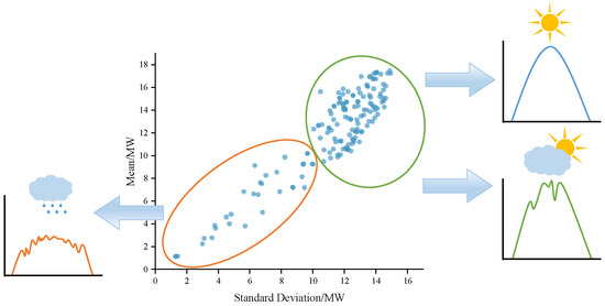
Figure 1.
Scatterplot of PV power mean and standard deviation.
PV power is strongly correlated with weather conditions, and the fluctuation amplitude, complexity of time series changes, and statistical distribution characteristics of power curves under different weather types differ significantly. The current inaccuracy of weather type clustering based on PV power time series is mainly due to the complex spatial and temporal characteristics of the power curves and the limitations of the existing clustering algorithms. As shown in Figure 1, among the commonly used statistical indicators, the mean and standard deviation can only portray the concentration trend and overall dispersion of the data. However, such scalar metrics are not capable of characterising the key dynamic properties of the power series:
- Ignoring fluctuation patterns and distribution patterns: The mean and standard deviation do not effectively capture the specific fluctuation patterns and statistical distribution patterns embedded in the power curve. This results in the fact that different weather types may have similar combinations of means and standard deviations—a cloudy day with high fluctuations versus a rainy day with high noise interference—while the same weather type may have significantly different means and standard deviations in different seasons, geographic regions, or power station conditions. The consequence is a homogenisation of the fluctuation pattern, where the characteristic ‘sawtooth’ high-frequency power fluctuations triggered by rapid cloud movement, which are characteristic of cloudy weather, may not be effectively differentiated from extreme weather events with sudden rises and falls in the statistical indicators.
- Loss of local features of the time series: These global statistics average out instantaneous changes and dilute local anomalies. Local power spikes due to brief clear skies against a background of cloudy or overcast weather have their instantaneous effects smoothed out by the mean, and their steep magnitude of change attenuated by the overall standard deviation, thus losing key information reflecting transient changes in the weather.
Therefore, in order to make up for the limitation that the mean and standard deviation can only measure the overall dispersion, and to portray the nonlinear dynamic characteristics and distribution pattern of the power curve more comprehensively. In this study, skewness, kurtosis, and sample entropy are introduced as the key feature indicators and Weighted Turning Point Density (WTPD) is proposed. WTPD strengthens the sensitivity to abrupt changes by weighting the extreme points, complements the shortcomings of the other indicators, and forms orthogonal and complementary dimensions with the other indicators. The following six feature indicators are used:
- Mean
The mean value characterises the average level of daily power output and reflects the overall impact of weather on the PV power system. The average daily power output is significantly higher on sunny days than on cloudy days due to sustained high irradiance, and intermediate on cloudy days.
- 2.
- Standard Deviation (Std)
The standard deviation describes the absolute intensity of fluctuations in the power series. Cloudy weather has frequent and abrupt changes in power due to cloud movement, and the standard deviation is usually higher than other weather types.
- 3.
- Weighted Turning Point Density(WTPD)
In order to quantify the fluctuation characteristics of the PV power curve, WTPD is introduced. By counting the number of peaks and valleys in the power curve and assigning weights according to the magnitude size of the local extreme points in the power curve, WTPD significantly strengthens sensitivity to transient mutation events such as sudden rises and falls in the power curve, and effectively captures local mutation information that are lost by the other indicators in the whole picture. WTPD is able to reflect the frequency and intensity of fluctuations more comprehensively through amplitude weighting, thus enhancing the ability to differentiate complex weather scenarios. The expression is as follows:
where is the indicator function, which is taken as 1 when the amplitude difference between adjacent peaks and troughs is , 3 and 0, otherwise, NH and NL denote the number of peaks and troughs that satisfy the condition, PH(i) and PL(j) denote the amplitude of the ith peak and jth trough that satisfy the condition, respectively, and T is the number of sampling points of the time series.
- 4.
- Skewness
Skewness is used to measure the asymmetry of the power distribution. The curve is approximately symmetrical (skewness close to 0) on clear days, while cloudy days may produce a right-skewed distribution (skewness > 0) due to transient shading.
- 5.
- Kurtosis
Kurtosis assesses the thickness of the tail of the power distribution. The curve is close to a normal distribution on sunny days and shows a low-peaked state on cloudy days due to smooth power output.
- 6.
- Sample Entropy(SE)
Sample entropy quantitatively describes the complexity of unstable sequences, which is proportional to the sequence complexity. SE denotes the sample entropy, and its expression is as follows:
where N denotes the length of the original sequence used to evaluate the entropy of the sample, m denotes the dimension of the reconstructed feature, and measures the local similarity of the sequence in a higher dimension m + 1, which captures the complexity of the sequence. is the number of times the distance between the ith template vector of length m + 1 and all other template vectors is less than r. measures the local similarity of the original sequence in dimension m, and is the number of times the distance between the ith template vector of length m and all other template vectors is less than r.
2.2. Multidimensional Volatility Characteristics Indicator System
In the clustering analysis of PV power time series, the six types of feature indicators selected in this paper portray the power series characteristics from different dimensions of output level, fluctuation intensity, local mutation, distribution pattern, and temporal complexity, respectively. Since the six selected feature indicators have different physical meanings and scales, directly adopting the original data for distance calculation will lead to an unbalanced contribution of each feature to the clustering results. In this paper, the Min-Max normalisation method is used to normalise the raw features. This method maps each feature value to the [0, 1] interval through linear transformation, effectively eliminating the influence of differences in magnitude on the distance calculation. After completing the feature normalisation, the six features are combined to form a six-dimensional feature vector. For any two daily power series samples xi and xj, their feature vectors can be expressed as:
Spectral clustering is a clustering method based on graph theory and algebraic graph theory, which is widely used in all kinds of clustering problems because of its advantages in dealing with complex data structures. The algorithm considers data points as vertices of the graph, constructs the graph through the similarity between data points, and transforms the clustering problem into the optimal division of the graph. Compared with traditional clustering algorithms, spectral clustering usually shows more robustness in dealing with arbitrarily shaped clusters and coping with the challenges of high-dimensional data.
A key issue in clustering PV power time series is accurately capturing the minute-scale ‘sawtooth’ power fluctuations characterised by rapid cloud movements. These high-frequency, non-stationary, sudden rises and falls are important markers for distinguishing key weather types. However, traditional distance metrics have significant limitations in dealing with such localised abrupt fluctuations. The global smoothing property of the Euclidean distance tends to average out the differences across the sequence, blunting the perception of locally occurring sharp power bursts and making it difficult to accurately measure the similarity between sequences in terms of key fluctuation patterns.
In order to construct a high-quality sample dataset suitable for PV station power prediction, the goal of this study is to clearly classify the historical PV power series into representative weather type categories—sunny, cloudy, and rainy—based on the level of power fluctuations. Constructing such a sample set that distinguishes between different fluctuation intensities is essential for training prediction models for specific weather patterns.
To achieve this goal and overcome the shortcomings of traditional distance metrics, this paper proposes an improved clustering distance method based on multidimensional fluctuation features and integrates it into a spectral clustering model to achieve the construction of a collection of samples of different fluctuation classes. The core of this method lies in the integrated use of multidimensional fluctuation features to refine the measure of similarity between sequences, especially to strengthen the ability to perceive local abrupt change patterns. This improved distance measure is integrated into the spectral clustering framework to form an improved spectral clustering model based on multidimensional fluctuation features. The ultimate goal of this model is to reasonably distinguish the power series patterns corresponding to sunny, cloudy, and rainy days, and to effectively construct high-quality sample sets reflecting different fluctuation levels with the following improved clustering distances:
where xi and xj denote the two sequences used for distance assessment, k denotes the index of the feature dimension with values ranging from one to six, corresponding to six feature indicators, and d(xi, xj) denotes the improved clustering distance. The distance value is positively correlated with the difference in fluctuation patterns of the sequences, and a smaller value indicates that the fluctuations of the two sequences are more similar.
3. PV Power Prediction Based on Combined NsT-BiLSTM Model
In response to the need for improved accuracy in PV power prediction, this study proposes a novel hybrid neural network architecture that integrates an improved Non-stationary Transformer with a BiLSTM. The traditional Transformer model has significant problems in PV power prediction: although the self-attention mechanism can capture global time-series dependence, it is prone to smoothing high-frequency fluctuating features (e.g., power dips triggered by cloud transients) due to its uniform weighting of historical information. This problem is especially prominent in PV situations, for example, the power sequence under cloudy weather often presents non-smooth, multi-peak mutation characteristics, and uniform attention weighting weakens the ability to recognise the local mutation. The Ns-Transformer effectively mitigates the problem by introducing the ‘de-smoothing’ module, which is the most effective way of characterising the local mutation. By introducing the ‘de-smoothing’ module, the Ns-Transformer effectively mitigates the degradation of temporal features caused by the self-attention mechanism of the traditional Transformer model. Meanwhile, in order to compensate for the deficiency of Transformer in local time series modelling, a BiLSTM network is introduced, whose bidirectional gating structure can synchronously capture the local dependence between historical and future directions, such as the rapid power recovery process caused by cloud gap radiation. The two modules are integrated through a cross-scale feature interaction layer: the Ns-Transformer outputs the global trend components, the BiLSTM extracts the local dynamic features, and these are adaptively weighted by the gating fusion mechanism to finally generate high-resolution prediction results. The specific improvements are as follows:
- Sequence smoothing process
In order to reduce the non-stationarity of each input sequence, the time dimension is normalised by a sliding window. The normalisation module can be represented as:
where n is the total number of input samples, is the variance of sample X, xd is the dth value in the fixed column of X, and is the mth value in the fixed column of .
For each input sequence , is obtained by the normalisation module as where k and d denote the length of the sequence and the number of variables, respectively.
- 2.
- De-smoothing attention
In order to achieve direct modelling of attention weights on un-smoothed time series data, this study designs an optimisation strategy based on statistical feature reconstruction. By constructing a multilayer perceptual network, the dynamic adjustment parameters and are resolved from the statistics and of the original non-smooth sequence X, and then the non-smooth information lost in the preprocessing stage is reintegrated into the attention computation framework. This de-smoothed attention architecture effectively improves the model’s prediction ability for the smoothed sequences while preserving the timing dependencies. The expression is:
where is the attention function, e is the input dimension, and is the activation function. To address the unique data characteristics of trend component prediction, this study adopts a sliding window strategy to dynamically correct the components using historical trend data.
- 3.
- Inverse normalisation module
After the model predicts future values of length O, the model output value is inversely transformed using the inverse normalisation module based on and :
where denotes the predicted value, denotes the inverse normalised value, and and denote the ith inverse normalised and normalised predicted value, respectively.
- 4.
- BiLSTM network
For the temporal characteristics of meteorological data, this study embeds a bidirectional LSTM layer between the Ns-Transformer encoder and the fully connected network on the basis of feature sequence , in order to effectively capture the long-term dependencies in the temporal features. The structure is specially designed for modelling complex temporal patterns in long time series. The design is capable of integrating the information of the previous and subsequent time points for prediction, effectively modelling the dynamic time-sequence correlations among meteorological elements, and significantly improving the model’s performance in extracting and identifying the spatio-temporal features of complex meteorological processes. From the technical implementation point of view, BiLSTM inherits the core mechanism of LSTM. Through the input gate, forgetting gate, and output gate mechanisms, information in the corresponding position is screened, the weight of the main information is strengthened, and the weight of irrelevant information is weakened, which can effectively capture the effective information of long time series data and effectively solves the gradient vanishing problem faced by the traditional recurrent neural network in the long time series modelling and the long-term dependence problem faced by traditional recurrent neural networks in long sequence modelling. The parameter update method is as follows:
where denotes the sigmoid activation function, tanh is the hyperbolic tangent activation function, xt denotes the input of the current time, ft, it, gt, and ot are the information of the forgetting gate, the input gate, the state update gate, and the output gate, respectively, and ct and ht are the memory unit and the hidden state of the current hidden layer, respectively. ct−1 and ht−1 are the memory cell and hidden layer state at time t − 1, respectively. W and b denote the weight matrix and bias vector of each gating unit, respectively.
As shown in Figure 2, the network achieves bidirectional feature extraction by processing forward and backward information streams of temporal data in parallel. The specific implementation contains two independent LSTM units that process the input sequences in the forward and backward directions, respectively, so as to comprehensively capture the temporal pattern features of each time node. Eventually, the network fuses the feature vectors extracted in both directions as input data for the subsequent fully connected network. The output layer of the architecture is designed as an n-dimensional space, where the prediction vector P represents the final output result of the BiLSTM model:
where P denotes the predicted output value, denotes the extracted features, and denotes the sequence of spatio-temporal features obtained after further extraction of temporal features by the BiLSTM module.
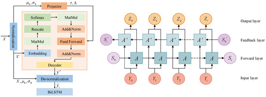
Figure 2.
NsT-BiLSTM overall architecture.
In Figure 2, the overall architecture of NsT-BiLSTM is demonstrated, and the whole architecture mainly consists of an embedding layer, encoder, and decoder. X denotes the input information matrix, X′ is the normalised feature matrix, and are the mean and standard deviation of X, respectively. y denotes the output feature matrix of the decoder and y′ denotes the matrix after inverse normalisation of y. and denote the de-smoothing factors.
4. Optimisation of Prediction Models Based on the DCS Algorithm
4.1. The Principle of DCS
Hyperparameter optimisation faces multiple challenges in PV power combination prediction models. The PV power sequence is highly non-stationary due to sudden weather changes, and traditional optimisation algorithms are prone to fall into local optima in high-dimensional parameter space, resulting in insufficient generalisation of the model under sudden-change scenarios. The optimal hyperparameter configurations corresponding to different weather types vary significantly, and it is difficult for static parameter settings to adapt to dynamic meteorological conditions, and so on. To address the challenges of hyperparameter optimisation in integrated prediction models, this study uses a new intelligent optimisation algorithm, DCS. The innovation of this method is that it breaks through the framework limitation of the classical differential evolutionary algorithm and applies a dual search strategy to achieve the synergistic optimisation of global exploration and local exploitation, which significantly improves the accuracy of model parameter configuration. The DCS consists of the following steps:
- 1.
- Random number initialisation: In the DCS optimisation algorithm, the optimisation process starts with a set of candidate solutions X, which are randomly generated between the upper bound U and the lower bound L of the optimisation problem.where denotes the element at position j in row i of the candidate solution X, denotes random data uniformly distributed in the interval (0, 1), and and denote the upper and lower bounds of the optimisation, respectively.
- 2.
- Differential knowledge learning: Differences are mainly manifested in the fact that some individuals have different rates of knowledge acquisition, and the adjustment of some dimensions is significantly larger than others, while others show a relatively uniform pattern of knowledge structure change, with a more consistent degree of adjustment in each dimension. In the following equation, parameter ηi,t is the individual’s quantitative knowledge acquisition rate qKR at the tth iteration, which can be expressed as:where the symbol denotes the rounding of the given value to the nearest integer, and is the individual’s coefficient at the tth iteration, which can be expressed as:where is the order of the ith individual at the start of the tth iteration.
- 3.
- Thinking strategies:
- (1)
- Convergent thinking: firstly, using the knowledge structure of the current optimal individual as a guiding basis; secondly, integrating the empirical contributions of two randomly selected team members. The algorithm can effectively guide the search process to converge towards the optimal solution while maintaining the diversity of the population. The strategy is formulated as follows:where is the best-performing individual at position d in the current iteration. denotes the best performer’s cognitive weight, which has a default value of 1, and is the individual’s w coefficient at the tth iteration. is the individual at position d randomly selected from and . is the coefficient of at iteration t. is the individual at position d randomly selected from and .
- (2)
- Divergent thinking: a new strategy was proposed and represented by the following equation:where denotes the element of the test vector at position d, i.e., the test member of , and denotes a Linnik-distributed random number generator with control parameters and .
- (3)
- Team diversity: Teams with changing individuals generate more diverse ideas and the algorithm replaces underperforming individuals with new ones. The formula for generating new individuals is as follows:where denotes the Mth test individual.
- 4.
- Boundary constraint processing: this ensures the feasibility of the solution space. When the candidate solutions generated during the optimisation process exceed the preset boundary in the dth dimension, the system will automatically adjust them to the maximum value allowed in that dimension, so as to ensure that all the solutions meet the constraints of the real problem. It is expressed by the following equation:
- 5.
- Retrospective assessment: Firstly, the evaluation indicator system is established as the reference standard for performance measurement, and subsequently, the development pattern and room for optimisation are identified through the systematic analysis of historical performance data. The formula for retrospective assessment is as follows:where denotes the ith individual in X at iteration. denotes the test member of , and denotes the ith individual at tth iteration. and are the target values of and , respectively. The formula for tracking the best performer is as follows:where denotes the best performing individual in the tth iteration, and and are the target values for and , respectively.
- 6.
- Adaptive function: in order to enable the optimisation algorithm to optimally adjust the hyperparameters of the combined prediction model based on the ideal state, this paper proposes the optimisation adaptive function for model optimisation convergence, whose expression is as follows:where denotes the fitness function, denotes the ith actual value, denotes the ith predicted value after model optimisation, and n denotes the length of the validation set sequence used to test the model optimisation performance.
4.2. The Theoretical Advantages of DCS
To adapt to parameter optimisation in multi-weather scenarios, the DCS constructs a “stage-adaptive and parameter-priority” dual-drive mechanism, which can match different weather patterns and locally adjust high-sensitivity parameters in stages. By contrast, the GA has a fixed strategy and thus struggles to adapt to weather-related parameter differences, while the BOA relies on prior information and tends to deviate in search direction when sudden weather changes occur. The DCS simultaneously adopts a “dual-population collaboration” design: the exploration population locks in the global weather parameter domain, and the correction population fine-tunes parameters at mutation points. The two populations interact dynamically to balance weather adaptation and power mutation capture. In comparison, the GA is prone to premature convergence in the late iteration stage, and the BOA lacks clear global–local switching conditions, resulting in poor adaptability to transitional weather. In terms of resource allocation, the DCS first performs parameter sensitivity clustering and then allocates resources on demand. However, the GA requires more iterations and exhibits slow convergence, while the BOA is prone to information transmission failure in high-dimensional spaces.
The overall architecture of this paper is as shown in the Figure 3.
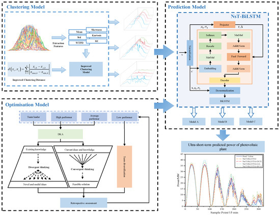
Figure 3.
Overall architecture.
5. Case Study
In order to assess the accuracy of the prediction method, this paper uses the root mean square error (RMSE) and mean absolute error (MAE) to assess the prediction results, and the standard formulas for the above accuracy metrics are, respectively:
where denotes the ith actual value, denotes the ith predicted value, n denotes the length of the sequence, and Cap denotes the total installed capacity of the PV site.
The data used in this study are from a PV power station with a total installed capacity of 40 MW in Jilin province, China, spanning from 1 January 2019 to 30 June 2019, with a temporal resolution of 15 min. The historical PV power data and its corresponding NWP data are selected, including the short-wave radiation, long-wave radiation, total precipitation, cloud cover, and temperature. After weather clustering, each weather type takes the last two days as the test set, and the rest are the training set. In order to objectively evaluate the prediction accuracy of the model, 100 experiments are conducted for each weather type, and the average value is taken as the final prediction value, which is analysed with the real value for error calculation. In this paper, various data preprocessing is performed, including data denoising, missing data interpolation, and normalisation.
5.1. Analysis of Clustering Results
In order to obtain historical samples with different fluctuation levels and construct a sample set of PV power, clustering is first performed based on historical PV power daily time series, and an improved clustering distance method that combines multidimensional fluctuation features with spectral clustering model is used to cluster historical samples of PV stations. In order to compare the clustering effect of different models, k-means and k-medoids clustering models are introduced for comparison.
Due to the complexity and variability of weather in practical engineering applications, this paper does not consider scenarios such as sunny to cloudy and sunny to rainy, and only divides the weather patterns into three categories, which are sunny, cloudy, and rainy. As shown in Figure 4, it can be seen that the curve fluctuations are similar under the same weather type. The curve fluctuations are very small in sunny days, and the curve fluctuations are very frequent and differ greatly from day to day on cloudy days as well as cloudy and rainy days. In order to verify the superiority of the spectral clustering method with improved clustering distance proposed in this paper, the clustering method proposed in this paper is compared with k-means and k-medoids clustering algorithms, and the profile coefficient is used as an evaluation index to evaluate the clustering results. The more the value tends to 1, the better the clustering effect; the more it tends to -1, the worse the clustering effect. The more concentrated the contour coefficient values are, the more similar the samples are to each other.
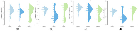
Figure 4.
Distribution of silhouette coefficients for different clustering methods: (a) k-means, (b) k-medoids, (c) spectral clustering–correlation coefficient, and (d) spectral clustering–improved distance.
In order to assess the accuracy of the clustering method, the clustering results were evaluated using the error value with the following expression:
where C denotes the number of days for clustering and R is the actual number of days. Table 1 shows the error values of different models for clustering, it can be seen that the average error value of the proposed model is the lowest, and the method gives the best clustering results.
As shown in Figure 5, which shows the contour coefficients of each sample cluster corresponding to different clustering models and distances, almost every clustering model leads to significantly different contour coefficients for the results of each class. From all the clustering results, the clustering algorithm based on improved cluster distance has significantly higher profile coefficient values and greater concentration than the other results. The clustering results of the samples using the clustering method proposed in this paper have a higher concentration of sunny-day profile coefficients around 0.4 and a higher concentration of cloudy- and rainy-day profile coefficients at 0.5, and both categories show higher and more concentrated values of profile coefficients than those of the other clustering methods. However, due to the variable irradiance on cloudy days and the fact that the curves are more similar to those on sunny days except during transitions, the similarity across samples and profile coefficients are low. Meanwhile, spectral clustering based on correlation coefficient distance is not effective in filtering different samples into different clusters, and its clustering effect is poor despite the large value of its profile coefficient.
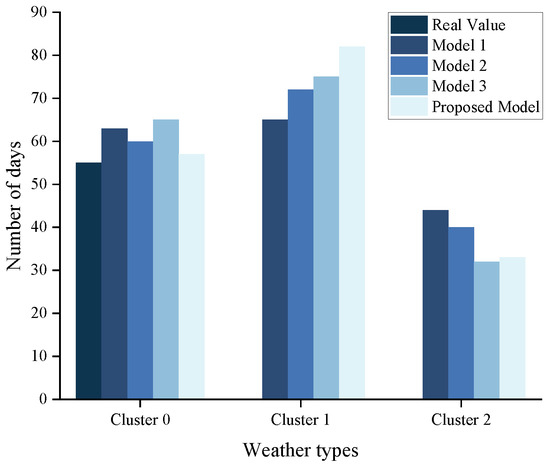
Figure 5.
Number of days per weather type for different clustering methods.
The improved clustering distance proposed in this study effectively filters the sunny, cloudy, and rainy day samples into corresponding clusters. In this study, Cluster 0 represents the sunny-day results, Cluster 1 represents the cloudy-day results, and Cluster 2 represents the rainy-day results. Table 2 demonstrates the values of the profile coefficients in each cluster, illustrating that the profile coefficient for sunny days is 0.3403, the profile coefficient for cloudy and rainy days is 0.3930, and the profile coefficient for cloudy days is the lowest, indicating that cloudy days comprise more samples with high fluctuation. As a result, the average profile coefficients for cloudy days are lower than the first two categories.
Table 2.
The error values of different models for clustering.
These samples with similar volatility processes were clustered into different clusters by other models, resulting in poor final clustering. However, the proposed improved model effectively avoids this phenomenon and ensures that the final clustering performance meets the goal of volatility sample filtering and construction. Figure 6 shows the clustering results corresponding to these models. The method proposed in this paper effectively distinguishes samples with different volatility levels and successfully achieves sample clustering.
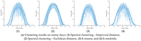
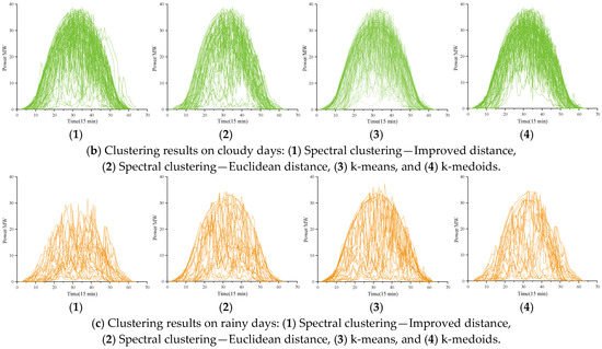
Figure 6.
Clustering results corresponding to different clustering methods and clustering distances.
To clarify the ranking of the significance of each feature’s contribution to clustering performance, this study employs the one-way analysis of variance (ANOVA) method to conduct a quantitative analysis of the clustering contribution degree of each feature index. Within the ANOVA analytical framework, the F-value is used to quantify the significance of differences in a single feature across different clustering categories: a larger F-value indicates a higher ratio of the feature’s inter-cluster differences to its intra-cluster differences, which in turn means stronger discriminative ability for clustering category boundaries and, correspondingly, a higher contribution degree to the clustering results. The specific calculation formula of the F-value is presented as follows:
where SSt is between-cluster variance, SSe is inter-cluster variance, dft is between-cluster degrees of freedom, and dfe is inter-cluster degrees of freedom.
Figure 7 presents the F-values corresponding to each feature. Among them, the feature SE exhibits the largest F-value, indicating that it is the indicator with the most significant inter-cluster differences among all features. SE is used to characterise the complexity and irregularity of PV output sequences; its high F-value intuitively reflects that there are significant differences in the fluctuation complexity of PV output across different clustering categories. Thus, this feature possesses the strongest ability to distinguish between clustering categories and serves as the feature with the highest contribution degree to clustering. The clustering contribution degree of feature WTPD ranks second only to that of SE. This indicator distinguishes different PV output scenarios effectively by counting the number of peaks and valleys in the power curve and assigning corresponding weights based on the amplitude of local extreme points in the power curve. The level of its F-value further confirms the important supporting role of this feature in the clustering results. The clustering contribution degree of feature mean ranks third. As a core indicator representing the average level of PV output, mean is a fundamental parameter for describing PV output types. Its F-value demonstrates the fundamental supporting value of this feature in the division of clustering categories. The clustering contribution degree of feature Std ranks fourth. As a classic indicator representing the degree of data dispersion, Std is used to measure the fluctuation amplitude of PV output. Its F-value indicates that there are distinguishable differences in the magnitude of output fluctuations across different clustering categories; however, the significance of these differences is slightly lower than that of the three features (SE, WTPD, and mean) mentioned above. In addition, the clustering contribution degrees of features skewness and kurtosis are relatively limited. Both of their F-values remain at a low level, which indicates that their ability to distinguish between clustering categories is weak, and their role in improving the overall clustering performance is relatively insignificant.
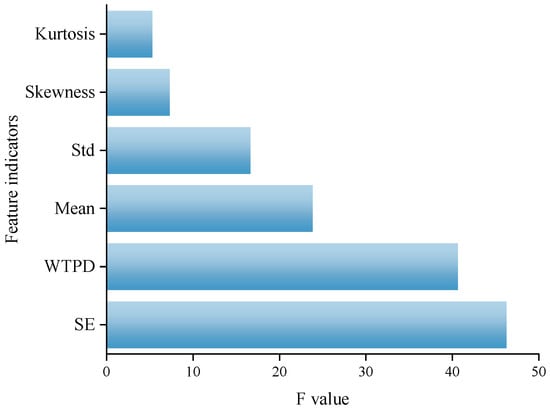
Figure 7.
F-value for each feature indicator.
5.2. Prediction Results
Comparison of Prediction Results Based on Different Clustering Models
In order to verify the effectiveness of the proposed framework, four clustering models (Spectral clustering—Improved distance, Spectral clustering—Euclidean distance, k-means, and k-medoids) combined with NsT-BiLSTM model are used in this study for PV power prediction, focusing on the prediction performance of different clustering preprocessing methods under three typical weather patterns, namely sunny, cloudy, and rainy days. Each model is defined as follows:
- (1)
- MA (Prediction based on Spectral clustering—Improved distance)
- (2)
- MB (Prediction based on Spectral clustering—Euclidean distance)
- (3)
- MC (Prediction based on k-means)
- (4)
- MD (Prediction based on k-medoids)
Based on the clustered PV data, each model is trained and predicted, respectively, and MAE and RMSE are used as the evaluation metrics. The specific results are shown in Table 3. The experiments show that the MA model proposed in this paper achieves the best overall prediction results on this dataset in combination with the NsT-BiLSTM model, which indicates that the improved distance metric can capture the nonlinear fluctuation characteristics of the meteorological data more accurately and effectively improve the clustering quality. The average errors of all clustered models are 0.0132 and 0.0153 lower than those of the unclustered benchmark model, which verifies the effectiveness of the ‘clustering before prediction’ strategy in modelling complex weather patterns. Under clear-sky conditions, the MA and MB models are able to effectively capture the power time-series characteristics due to the small fluctuations of irradiance, cloudiness, and temperature, and their prediction accuracies are significantly better than those of the other models. However, under non-sunny conditions, the prediction is made more difficult by intermittent meteorological fluctuations, and the prediction errors of all models increase. Among them, the prediction based on the clustering model proposed in this paper still maintains the optimal performance, and its MAE and RMSE are reduced by 0.0304 and 0.0316 on average compared with the unclustered model.
Table 3.
Silhouette coefficients of each category for different clustering methods.
The results show that the predictions using the four weather clustering methods described above show that the overall error is reduced regardless of the method used. The power prediction model based on a spectral clustering model with multidimensional fluctuation feature metrics maintains optimal robustness under all three weather conditions, and the method reduces the overall MAE and RMSE by 0.01605 and 0.0369, respectively. The improvement is particularly significant in the non-sunny scenarios, where the prediction of complex weather conditions is more accurate than the direct prediction results of the unclustered model.
5.3. Prediction Results of Ablation Experiments
In order to verify the applicability of the proposed method in PV power prediction for different weather types, this paper comparatively analyses the PV power prediction performance from M1 to M2, comparing each prediction method based on the clustering model and not based on the clustering model, as shown in Table 4. Based on the fluctuating division of PV power, this paper establishes a PV subset power prediction model for each PV subset using the DCS-NsT-BiLSTM combined architecture. The power of each fluctuating PV power subset is predicted separately, and finally the power prediction for the whole scene is achieved. In order to compare with the DCS optimisation algorithm used, several other optimisation algorithms including the genetic algorithm (GA) and the Bayesian optimisation algorithm (BOA), are also presented in this paper.
Table 4.
Evaluation metrics for prediction error based on different clustering models.
The prediction curves of each method are shown in Figure 9. MAE and RMSE of the prediction results are shown in Table 5. The experimental results show that the prediction results based on the clustering model are closer to the real values than those not based on clustering. Combining Figure 8 and Table 5, it can be observed that, across all weather types, the accuracy of all models is lower on cloudy and rainy days than on sunny days. It is because the weather conditions on cloudy days are more chaotic, which affects the accuracy. The prediction performance of the model in this paper is better than the other models and the prediction performance is significantly improved. In particular, the predicted and real values of PV power match better on sunny days, and the prediction results on cloudy and rainy days are also acceptable.
Table 5.
Methodological specifics.
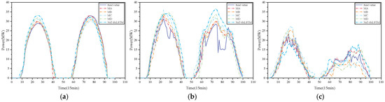
Figure 8.
Prediction results based on different clustering models: (a) sunny days, (b) cloudy days, and (c) rainy days.
For sunny-day predictions under the clustering-based model, combined with Figure 8, the predicted power curve of each model are closer to the real power curves, which indicates that each prediction model perform well on sequences with small fluctuation frequency and can accurately identify the fluctuating characteristics of PV power under this weather. Model M1 is the closest to the real value and has the smallest prediction error with MAE of 0.0723 and RMSE of 0.0989. By comparing models M2 and M3, it can be seen that both MAE and RMSE improve by more than 2%, demonstrating that the DCS optimisation is effective in optimising the hyperparameters of the model and improving the prediction accuracy of the model.
For cloudy-sky predictions under the clustering-based model, the proposed model is able to sense the trend and respond with high accuracy when the weather conditions change suddenly. The NsT-BiLSTM model used in M1 strengthens the extraction of local features for cloud masking events through the spatio-temporal attention mechanism. The prediction results of the unoptimised models M7 and M8 are not as good as expected, which may be due to the fact that the hyperparameters, such as the learning rate, are not adapted to this weather type. The proposed model in this paper improves the MAE and RMSE by 0.0404 and 0.0089 over M2, and by 0.0236 and 0.0054 over M3, respectively.
For the rainy-day predictions under the clustering-based model, the overall PV power output values are much smaller than in sunny and cloudy weather types, and the PV power varies frequently due to the higher randomness and low irradiance. The power curves obtained by the impermeable prediction models deviate from the true value curves, resulting in poor prediction. The MAE of the proposed model is reduced by 0.0253, 0.0031, 0.0334, 0.034, and 0.0241 compared to the other models M2, M3, M4, M5, and M6, respectively.
As shown in Table 6, for PV power prediction across diverse weather types, the 95% confidence intervals characterise the fluctuation range of results obtained from 100 repeated experiments using the proposed method. Narrower interval signify higher stability. Specifically, the 95% confidence interval of RMSE under sunny days is (0.0969, 0.1009), and that of MAE is (0.0709, 0.0737), both exhibiting extremely narrow ranges. Similarly, the 95% confidence interval of RMSE under cloudy days (0.1085, 0.1093), and that of MAE under rainy days (0.0989, 0.0995), also showing narrow and concentrated ranges. These findings indicate that after 100 repeated experiments, the prediction results of the proposed method under sunny, cloudy, and rainy scenarios exhibit slight fluctuations and high consistency, thereby demonstrating reliable stability across different weather types and achieving excellent overall prediction performance. The mean and confidence intervals of RMSE and MAE for the proposed method in different weather types are as Table 7.
Table 6.
Evaluation indices of clustering model-based PV power prediction error under different weather types.
Table 7.
The mean and confidence intervals of RMSE and MAE for the proposed method in different weather types.
This paper shows the optimisation results of each optimisation algorithm under different PV weather types. In order to evaluate the training effect of different optimisation algorithms on the NsT-BiLSTM model, this study compares the performance of DCS, GA, and BOA. The fitness curves of the three, with the number of iterations on the horizontal axis and the fitness value on the vertical axis, are illustrated in Figure 9, which shows that the DCS algorithm can complete the main optimisation task within 7 iterations, while BOA and GA require nearly 10 or more iterations to achieve lower loss values. In each case, the optimisation algorithms proposed in this paper corresponds to significantly lower fitness values than the other compared algorithms.
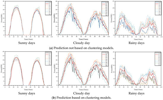
Figure 9.
Prediction results of the ablation experiments.
After the above model optimisation, this paper further evaluates the power prediction error evaluation indexes corresponding to different power prediction models under different PV weather conditions, and the statistical results are shown in Figure 10. Under the three types of fluctuating weather conditions, the accuracy of PV power prediction shows some variability, and there are some correlations between the prediction errors and power levels. The accuracy of PV power prediction is lower in high-power scenarios and higher in more volatile weather conditions. Fitness curves for different optimisation methods are as Figure 10. Evaluation indices of prediction error based on clustering models under different weather types are as Figure 11.
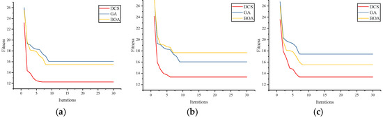
Figure 10.
Fitness curves for different optimisation methods: (a) sunny days, (b) cloudy days, and (c) rainy days.
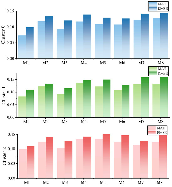
Figure 11.
Evaluation indices of prediction error based on clustering models under different weather types.
6. Conclusions
This study proposes a meteorological type clustering method based on multi-dimensional feature fusion, introduces an improved clustering distance metric, and constructs PV output sample sets corresponding to different meteorological types. For each meteorological type, a joint NsT-BiLSTM prediction model is established, and a novel intelligent optimisation algorithm, the DCS, is adopted to optimise the model. The research conclusions are as follows:
- To address the insufficient characterisation of meteorological features in traditional PV sequence clustering methods, this study combines the climate type of the PV power station, proposes an improved clustering distance metric based on the multi-dimensional feature fusion strategy, and embeds it into the spectral clustering model for clustering analysis of historical PV output data. This method effectively improves the accuracy of weather typing and resolves the defect of insufficient sensitivity of traditional clustering models to high-dimensional non-stationary data, thereby laying a reliable data foundation for subsequent PV power prediction.
- This study conducts short-term power prediction research on PV sample sets of different meteorological types based on the NsT-BiLSTM model. Specifically, the Ns-Transformer module is used to extract the temporal–spatial dual-dimensional features of the input information of each sample set, and the BiLSTM model is employed to capture the temporal dependence of historical PV output. On this basis, a dedicated power prediction model for each sub-cluster type of the PV power station is constructed. This model not only significantly improves the accuracy of PV power prediction but also effectively remedies the performance shortcomings of traditional Transformer models in non-stationary sequence processing.
- Regarding the problems of slow convergence speed and insufficient model generalisation performance in the optimisation process of high-dimensional parameter spaces, this study proposes a novel DCS optimisation model to perform hyperparameter optimisation for the NsT-BiLSTM hybrid model. This optimisation model can accelerate the convergence rate of the model toward the local optimal region and further improve the accuracy of PV power prediction. Experimental results show that the proposed DCS-NsT-BiLSTM hybrid model achieves the highest prediction accuracy, with its mean absolute error (MAE) and root mean square error (RMSE) reduced by 0.0369 and 0.0463, respectively, compared with the unoptimized NsT-BiLSTM model.
7. Future Research Plan
This study primarily focuses on photovoltaic power forecasting under normal weather conditions, which represent the most prevalent scenarios in practice and ensure the stability and feasibility of the model in real-world applications. Future work will be extended to transitional and extreme weather conditions; however, this direction entails considerable challenges, including limited data availability, rapid power fluctuations, and stringent requirements for computational efficiency and real-time implementation. Addressing these issues—achieving effective modelling under scarce data, while balancing predictive accuracy, computational efficiency, and generalisation ability—will constitute the core difficulty and emphasis of subsequent research.
Author Contributions
Conceptualization, M.Y. and S.G.; methodology, S.G.; software, S.G.; validation, M.Y., S.G. and J.C.; formal analysis, S.G. and W.X.; investigation, W.H. and K.W.; resources, J.C.; data curation, S.G.; writing—original draft preparation, S.G.; writing—review and editing, M.Y.; visualisation, J.C. and W.H.; supervision, M.Y.; project administration, K.W. and W.X.; funding acquisition, M.Y. All authors have read and agreed to the published version of the manuscript.
Funding
This research work is supported by the project “Analysis and Application of Spatiotemporal Evolution Law of Long-Period Process of Extreme Weather and Its Influence on New Energy Operation” (4000-202455070A-1-1-ZN).
Data Availability Statement
The datasets presented in this article are unavailable due to privacy restrictions.
Conflicts of Interest
Authors Wei He, Kang Wu, and Wei Xu were employed by the State Grid Corporation of China. The remaining authors declare that the research was conducted in the absence of any commercial or financial relationships that could be construed as a potential conflict of interest.
Abbreviations
The following abbreviations are used in this manuscript:
| PV | Photovoltaic |
| DCS-NsT-BiLSTM | Non-Stationary Transformer-bidirectional Long Short-Term Memory network optimized with Differentiated Creative Search |
| FCM | Fuzzy C-means clustering |
| NWP | Numerical weather prediction |
| SVM | Support Vector Machine |
| WTPD | Weighted Turning Point Density |
| RMSE | Root mean square error |
| MAE | Mean absolute error |
| GA | Genetic algorithm |
| BOA | Bayesian optimisation algorithm |
| TCN | Temporal convolutional network |
| MLP | Multilayer perceptron |
| KNN | K-nearest neighbours algorithm |
| ELM | Extreme learning machine |
| LSTM | Long Short-Term Memory |
| BP | Back propagation neural network |
| LSSVM | Least square support vector machine |
| WNN | Wavelet neural network |
| GRU | Gated recurrent unit |
| XGBoost | Extreme gradient boosting |
References
- Yang, M.; Wang, D.; Zhang, W.; Yv, X. A centralized power prediction method for large-scale wind power clusters based on dynamic graph neural network. Energy 2024, 310, 133210. [Google Scholar] [CrossRef]
- Zhou, X.; Chen, S.; Lu, Z.; Huang, Y. Technology features of the new generation power system in China. Proc. CSEE 2018, 38, 1893–1904. [Google Scholar]
- National Energy Administration. The Country’s Cumulative Installed Power Generation Capacity Is About 3.16 Billion Kilowatts; National Energy Administration: Beijing, China, 2024. [Google Scholar]
- Wang, K.; Qi, X.; Liu, H. A comparison of day-ahead photovoltaic power forecasting models based on deep learning neural network. Appl. Energy 2019, 251, 113315. [Google Scholar] [CrossRef]
- Shi, K.; Zhang, D.; Han, X.; Xie, Z. Digital twin model of photovoltaic power generation prediction based on LSTM and transfer learning. Power Syst. Technol. 2022, 46, 1363–1372. [Google Scholar]
- Simeunović, J.; Schubnel, B.; Alet, P.J.; Carrillo, R.E. Spatio-temporal graph neural networks for multisite PV power forecasting. IEEE Trans. Sustain. Energy 2021, 13, 1210–1220. [Google Scholar] [CrossRef]
- Yang, M.; Guo, Y.; Wang, B.; Chai, R. A day-ahead wind speed correction method: Enhancing wind speed forecasting accuracy using a strategy combining dynamic feature weighting with multisource information and dynamic matching with improved similarity function. Expert Syst. Appl. 2025, 263, 125724. [Google Scholar] [CrossRef]
- Zhen, Z.; Liu, J.; Zhang, Z.; Wang, F.; Chai, H.; Yu, Y.; Lu, X.; Wang, T.; Lin, Y. Deep learning based surface irradiance mapping model for solar PV power forecasting using sky image. IEEE Trans. Ind. Appl. 2020, 56, 3385–3396. [Google Scholar] [CrossRef]
- Wang, H.; Yi, H.; Peng, J.; Wang, G.; Liu, Y.; Jiang, H.; Liu, W. Deterministic and probabilistic forecasting of photovoltaic power based on deep convolutional neural network. Energy Convers. Manag. 2017, 153, 409–422. [Google Scholar] [CrossRef]
- Yang, M.; Jiang, Y.; Xu, C.; Wang, B.; Wang, Z.; Su, X. Day-ahead wind farm cluster power prediction based on trend categorization and spatial information integration model. Appl. Energy 2025, 388, 125580. [Google Scholar] [CrossRef]
- Hann, T.H.; Steurer, E. Much ado about nothing? Exchange rate forecasting: Neural networks vs. linear models using monthly and weekly data. Neurocomputing 1996, 10, 323–339. [Google Scholar] [CrossRef]
- De Giorgi, M.G.; Malvoni, M.; Congedo, P.M. Comparison of strategies for multi-step ahead photovoltaic power forecasting models based on hybrid group method of data handling networks and least square support vector machine. Energy 2016, 107, 360–373. [Google Scholar] [CrossRef]
- Başakın, E.E.; Ekmekcioğlu, Ö.; Özger, M. Developing a novel approach for missing data imputation of solar radiation: A hybrid differential evolution algorithm based extreme gradient boosting model. Energy Convers. Manag. 2023, 280, 116780. [Google Scholar] [CrossRef]
- Zhu, J.; He, Y.; Yang, X.; Yang, S. Ultra-short-term wind power probabilistic forecasting based on an evolutionary non-crossing multi-output quantile regression deep neural network. Energy. Convers. Manag. 2024, 301, 118062. [Google Scholar] [CrossRef]
- Yang, M.; Huang, Y.; Xu, C.; Liu, C.; Dai, B. Review of several key processes in wind power forecasting: Mathematical formulations, scientific problems, and logical relations. Appl. Energy 2025, 377, 124631. [Google Scholar] [CrossRef]
- Mirza, A.F.; Mansoor, M.; Usman, M.; Ling, Q. Hybrid Inception-embedded deep neural network ResNet for short and medium-term PV-Wind forecasting. Energy Convers. Manag. 2023, 294, 117574. [Google Scholar] [CrossRef]
- Zhu, J.; Li, M.; Luo, L.; Zhang, B.; Cui, M.; Yu, L. Short-term PV power forecast methodology based on multi-scale fluctuation characteristics extraction. Renew. Energy 2023, 208, 141–151. [Google Scholar] [CrossRef]
- Viet, D.T.; Phuong, V.V.; Duong, M.Q.; Tran, Q.T. Models for short-term wind power forecasting based on improved artificial neural network using particle swarm optimization and genetic algorithms. Energies 2020, 13, 2873. [Google Scholar] [CrossRef]
- Peng, X.; Wang, H.; Lang, J.; Li, W.; Xu, Q.; Zhang, Z.; Cai, T.; Duan, S.; Liu, F.; Li, C. EALSTM-QR: Interval wind-power prediction model based on numerical weather prediction and deep learning. Energy 2021, 220, 119692. [Google Scholar] [CrossRef]
- Wu, Y.K.; Phan, Q.T.; Zhong, Y.J. Overview of day-ahead solar power forecasts based on weather classifications and a case study in Taiwan. IEEE Trans. Ind. Appl. 2023, 60, 1409–1423. [Google Scholar] [CrossRef]
- Ye, L.; Pei, M.; Lu, P.; Zhao, J.; He, B. Short-term PV power portfolio prediction method based on weather modelling. Autom. Electr. Power Syst. 2021, 45, 44–54. [Google Scholar]
- Zhang, M.; Han, Y.; Wang, C.; Yang, P.; Wang, C.; Zalhaf, M.S. Ultra-short-term photovoltaic power prediction based on similar day clustering and temporal convolutional network with bidirectional long short-term memory model: A case study using DKASC data. Appl. Energy 2024, 375, 124085. [Google Scholar] [CrossRef]
- Zheng, L.; Su, R.; Sun, X.; Guo, S. Historical PV-output characteristic extraction based weather-type classification strategy and its forecasting method for the day-ahead prediction of PV output. Energy 2023, 271, 127009. [Google Scholar] [CrossRef]
- Guan, L.; Zhao, Q.; Zhou, B.; Lv, Y.; Zhao, W.; Yao, W. Application of multiscale cluster analysis based modelling and prediction of PV power characteristics. Autom. Electr. Power Syst. 2018, 42, 24–30. [Google Scholar]
- Wang, F.; Zhang, Z.; Liu, C.; Yu, Y.; Pang, S.; Duić, N.; Shafie-Khah, M.; Catalão, J.P. Generative adversarial networks and convolutional neural networks based weather classification model for day ahead short-term photovoltaic power forecasting. Energy Convers. Manag. 2019, 181, 443–462. [Google Scholar] [CrossRef]
- Jamal, T.; Carter, C.; Schmidt, T.; Shafiullah, G.; Calais, M.; Urmee, T. An energy flow simulation tool for incorporating short term PV forecasting in a diesel-PV-battery off-grid power supply system. Appl. Energy 2019, 254, 113718. [Google Scholar] [CrossRef]
- Han, L.; Zhang, R.; Wang, X.; Bao, A.; Jing, H. Multi-step wind power forecast based on VMD-LSTM. IET Renew. Power Gener. 2019, 13, 1690–1700. [Google Scholar] [CrossRef]
- Gao, M.; Li, J.; Hong, F.; Long, D. Day-ahead power forecasting in a large-scale photovoltaic plant based on weather classification using LSTM. Energy 2019, 187, 115838. [Google Scholar] [CrossRef]
- Behera, M.K.; Nayak, N. A comparative study on short-term PV power forecasting using decomposition based optimized extreme learning machine algorithm. Eng. Sci. Technol. Int. J. 2020, 23, 156–167. [Google Scholar] [CrossRef]
- Niu, Y.; Wang, J.; Zhang, Z.; Cao, Y.; Yan, P.; Li, Z. Amplify seasonality, prioritize meteorological: Strengthening seasonal correlation in photovoltaic forecasting with dual-layer hierarchical attention. Appl. Energy 2025, 394, 126104. [Google Scholar] [CrossRef]
Disclaimer/Publisher’s Note: The statements, opinions and data contained in all publications are solely those of the individual author(s) and contributor(s) and not of MDPI and/or the editor(s). MDPI and/or the editor(s) disclaim responsibility for any injury to people or property resulting from any ideas, methods, instructions or products referred to in the content. |
© 2025 by the authors. Licensee MDPI, Basel, Switzerland. This article is an open access article distributed under the terms and conditions of the Creative Commons Attribution (CC BY) license (https://creativecommons.org/licenses/by/4.0/).