Abstract
Inverse problems are ubiquitous across many scientific fields, and involve the determination of the causes or parameters of a system from observations of its effects or outputs. These problems have been deeply studied through the use of simulated data, thereby under the lens of simulation-based inference. Recently, the natural combination of Continuous Normalizing Flows (CNFs) and Flow Matching Posterior Estimation (FMPE) has emerged as a novel, powerful, and scalable posterior estimator, capable of inferring the distribution of free parameters in a significantly reduced computational time compared to conventional techniques. While CNFs provide substantial flexibility in designing machine learning solutions, modeling decisions during their implementation can strongly influence predictive performance. To the best of our knowledge, no prior work has systematically analyzed how such modeling choices affect the robustness of posterior estimates in this framework. The aim of this work is to address this research gap by investigating the sensitivity of CNFs trained with FMPE under different modeling decisions, including data preprocessing, noise conditioning, and noisy observations. As a case study, we consider atmospheric retrieval of exoplanets and perform an extensive experimental campaign on the Ariel Data Challenge 2023 dataset. Through a comprehensive posterior evaluation framework, we demonstrate that (i) Z-score normalization outperforms min–max scaling across tasks; (ii) noise conditioning improves accuracy, coverage, and uncertainty estimation; and (iii) noisy observations significantly degrade predictive performance, thus underscoring reduced robustness under the assumed noise conditions.
1. Introduction
Inverse problems arise across many scientific disciplines and involve inferring unknown parameters or latent causes from observable data [1]. They are called inverse because they reverse the usual forward direction of modeling, where we predict outcomes from known parameters. Simulation-based inference (SBI) has become a popular framework for solving such inverse problems by relying on a statistical model with unknown or uncertain parameters [2] for which we want to estimate the corresponding posterior distribution, especially when the likelihood function is analytically intractable and computationally unfeasible. Neural SBI methods have emerged as a powerful likelihood-free class of SBI techniques exploiting the underlying amortized inference paradigm in which the initial cost of model training on a massive amount of simulated data is traded for a scalable and computationally efficient inference framework for posterior estimation on new unseen samples [3]. In this sense, recent advances like Flow Matching Posterior Estimation (FMPE [4]) have enabled the adaptation of modern deep generative models, such as Continuous Normalizing Flows (CNFs [5]), thus providing an attractive solution for complex posterior estimation tasks, thanks to remarkable properties including asymptotic exactness, flexibility, scalability, and principled uncertainty quantification [6].
Beyond methodological innovation [4,7], only very few recent works have begun to examine the sensitivity of neural posterior estimation (NPE) pipelines to modeling choices. For instance, preprocessing strategies such as dimensionality reduction were shown not to compromise posterior accuracy in X-ray spectral fitting [8], while new frameworks like robust neural posterior estimation (RNPE) [9] explicitly address posterior degradation under model misspecification. Neural posterior estimators, particularly those relying on deep architectures, are notoriously sensitive to a wide array of modeling choices (e.g., data preprocessing, input data uncertainty, noisy observations, etc.) that can significantly influence convergence behavior, estimation accuracy, and generalization [7,10].
The aim of this work is to address this research gap by presenting a systematic investigation of CNF sensitivity within the FMPE framework. As a compelling scientific case study, we consider exoplanetary atmospheric retrieval, a well-known inverse problem in astrophysics and planetary science, where normalizing flows are established as the state-of-the-art neural-based posterior estimator [11,12,13,14,15]. Moreover, the simulation-based nature of this problem provides a natural setting for conducting a thorough sensitivity analysis, enabling the controlled evaluation of modeling choices and their impact on posterior estimation. The major contributions of this work are the following:
- We conduct an extensive experimental campaign on the Ariel Data Challenge (ADC) 2023 dataset [16], considering thousands of CNF configurations with variations in input data, preprocessing strategies, network architectures, and optimization parameters.
- We evaluate the performance of CNFs trained with FMPE and the estimated posterior distributions through an extensive posterior evaluation framework encompassing prediction errors, calibration, uncertainty quantification, and coverage analysis.
- We perform a systematic comparison to assess the influence of sensitive modeling decisions on model performance. These include (i) min–max scaling versus Z-score normalization; (ii) noise conditioning, and (iii) robustness under perturbation noise.
- We identify principled design choices prioritizing key predictive qualities, thereby enhancing the robustness and reliability of simulation-based posterior inference using CNFs.
To the best of our knowledge, there is no prior work which performs a systematic analysis related to the abovementioned modeling choices affecting posterior robustness of CNFs trained with FMPE, especially in critical domains such as astrophysics, where unreliable posteriors might compromise significant scientific conclusions. The remainder of the paper is organized as follows. Section 2 provides a theoretical overview of simulation-based atmospheric retrieval, FMPE, and sensitive modeling decisions under investigation. Section 3 details the experimental setup, including the dataset preparation, model training, inference, and evaluation. Section 4 discusses the experimental results about the influence of the investigated modeling decisions. Conclusions are summarized in Section 5.
2. Methods
2.1. Simulation-Based Atmospheric Retrieval
In simulation-based inference (SBI), a simulator is a computer program that accepts a parameter vector as input, sequentially samples internal latent variables , and returns an observable output data vector . The parameters are much lower-dimensional than the data x (i.e., ), which is often associated with a complicated domain. The likelihood function is implicitly defined by the simulator as:
where is the joint probability density of data x and latent variables z. The goal of SBI—also known as likelihood-free inference—is to perform Bayesian inference (i.e., posterior estimation) without requiring numerical evaluation of the likelihood function [17], which is generally intractable due to the marginalization over the latent space of the simulator. This is translated into the estimation of the posterior distribution , defined as follows:
where the prior probability distribution encapsulates the initial assumptions about the model parameters .
In this work, we consider atmospheric retrieval of exoplanets, as has been deeply studied through the extensive use of simulated data, due to the lack of a sufficient volume of uncorrupted observations. Thus, the vector represents the set of atmospheric features over the parameter space and corresponds to an atmospheric spectrum (transmission, emission, or reflection) [18]. A so-called forward model simulates exoplanet spectra based on assumed atmospheric parameters . It solves the radiative transfer equation to produce a theoretical spectrum x, which can then be processed to resemble real observations [19]. Because of the complex, non-linear nature of the underlying physics and chemistry, retrieving from x is an ill-posed inverse problem, often leading to degeneracies, where multiple atmospheric scenarios yield similar spectra [16].
2.2. Flow Matching Posterior Estimation
To remain consistent with the existing literature, we adopt the notation introduced in [4,7] and refer the reader to the original works for technical terminology. Given a probability density path (i.e., a time-dependent probability density function), and a time-dependent vector field, , a vector field can be used to construct a time-dependent diffeomorphic map, called a flow, , defined via the ordinary differential equation (ODE):
The trajectories are computed by integrating the aforementioned ODE. The final posterior density is given by
where denotes the push-forward operator which describes the transformation of probability densities through time and invertible maps, the term div denotes the divergence operator, and denotes the additional context (at least including the observations). The vector field is typically modelled with a CNF [5], denoted with , where are its learnable parameters. Flow Matching (FM; [7]) provides a simulation-free framework for learning the parameters of a CNF, and its objective consists of regressing onto a target vector field that induces a desired probability path with and , where p is the source distribution (e.g., an isotropic Gaussian), and q is the unknown target distribution:
where the symbol denotes the expectation operator.
The standard FM objective is intractable without a prior definition of the probability path and vector field . Within the context of SBI, a sample-conditional formulation of FM (SCFM) has been introduced by the authors in [4], which drastically simplifies the definitions of and , by introducing a conditional objective providing equivalent gradients to the FM objective. Given a sample-conditional probability path at time t and the corresponding target vector field , the SCFM loss is defined as:
where the time t is sampled from a uniform distribution , is a reference posterior sample conditioned on x, and is the learnable vector field at time t for observation x.
A possible choice for the sample-conditional probability paths is given by the family of Gaussian paths:
parameterized by time-dependent means and standard deviations , subject to boundary conditions. The conditional Optimal Transport (OT) defines a linear change in time of and :
This leads to the sample-conditional vector field defined as follows:
Therefore, a novel sample can be generated from the target distribution by (i) drawing a sample from the source distribution , and (ii) solving the ODE determined in (3) through multiple neural function evaluations (NFEs; forward passes of a neural network). FMPE [4] enables CNFs to SBI by applying the Bayes’ theorem, thereby eliminating the intractable expectation over the unknown posterior in (6). Following these considerations, the SCFM loss can be replaced with the FMPE loss, defined as:
which can be easily minimized over samples obtained by (i) sampling from the prior (i.e., ), and (ii) simulating data x corresponding to (i.e., ). Intuitively, the CNF operates by progressively transforming samples from a simple base distribution through a learned time-dependent vector field, which guides the evolution of data points toward the desired posterior distribution of atmospheric parameters. Furthermore, the uniform time prior distribution can be generalized to a power-law prior distribution [4]. Regulating can further improve the learning capacity of CNFs by putting more training effort on complex transitions of the probability density , or equivalently, on the estimation of the time-dependent vector field .
2.3. Identification of Sensitive Modeling Choices
2.3.1. Data Normalization
Data normalization is a major preprocessing step in machine learning (ML) workflows, which may potentially affect convergence and generalization performance during model training and evaluation, respectively. The basic idea behind data normalization is to transform data from its original domain to a representation space more amenable to ML algorithms, ensuring that all input variables contribute comparably to the learning process. The most common data normalization strategies are min–max scaling and Z-score normalization. Here, we consider the feature-wise formulation of data normalization, instead of the sample-wise formulation where statistics are computed on a per-sample basis. Min–max scaling, also known as feature normalization, is a linear transformation technique that rescales numerical features to a fixed range, typically . Given a dataset , where n is the number of samples and m is the number of features, min–max scaling transforms each feature as:
where denotes the j-th feature column. While preserving the original relationships within the data, min–max scaling is sensitive to outliers, as extreme values in distort the denominator , compressing non-outlier values into a narrow range. This phenomenon could potentially degrade model performance and lead to poor model generalization. A more robust alternative is Z-score normalization (also known as standardization):
where and are the mean and standard deviation of the j-th feature. Standardization mitigates outlier influence by centering and scaling data relative to statistical moments rather than extrema. This characteristic enhances convergence in gradient-based optimization methods.
2.3.2. Explicit Incorporation of Input Data Uncertainty
Accurate quantification of uncertainty in ML models is crucial for ensuring reliable and safe predictions [20]. Explicit modeling of input uncertainty and noise could enhance model robustness by providing additional information for prediction tasks in scenarios where the magnitude of input uncertainty is known a priori [21]. Within the context of simulation-based atmospheric retrieval, modern implementations of forward models (e.g., Alfnoor [22]) can provide wavelength-dependent uncertainty estimates that incorporate various nuisance factors, including binning schemes, observational conditions, and diverse sources of corruption inherent in forward modeling processes. In real-world cases, instead, the signal-to-noise ratio (SNR) can be thought of as a measure of input data uncertainty. This information can be easily incorporated as additional input to neural networks acting as retrieval tools, allowing for the creation of a conditional posterior sampler, where the input data uncertainty is reasonably propagated throughout the network. Hereafter, we refer to the explicit incorporation of input uncertainty estimates into the retrieval process also as noise conditioning.
2.3.3. Training CNFs on Synthetic Data
Synthetic data has emerged as a promising solution to the data scarcity problem in deep learning [23]. However, a critical challenge hindering broader adoption is the reality gap, referred to as the performance discrepancy that occurs when models trained on synthetic data are deployed on real-world data. Within the context of real-world atmospheric retrieval, observers often receive corrupted observations (due to instrumental errors, limited spectroscopic coverage, etc.), which further complicates the retrieval task [16]. To measure the influence of realistic samples over ideal samples in retrieval performance, a realistic dataset can be constructed by augmenting ideal transmission spectra originated from forward models. A naive approach to produce more realistic observations consists of randomly perturbing the ideal transmission spectra with additive noise. We exploit the wavelength-dependent uncertainties produced by the simulator for each transmission spectrum s, and assume a sample-conditional multivariate Gaussian distribution as a noise model. Therefore, the realistic transmission spectra can be sampled from , or equivalently, can be defined as , where is a random noise vector drawn from , and m is the dimensionality of the theoretical transmission spectra. This ensures that CNFs trained with FMPE are not limited to ideal data, allowing assessment under perturbed conditions.
3. Experiments
3.1. Dataset
The 2023 edition of the ADC [16] represents a particular instance of simulation-based inference, aimed at advancing atmospheric retrieval methodologies in preparation for the ESA-Ariel space mission’s first light [24]. The ADC2023 dataset is an open-source simulated database with 41,423 samples including the following:
- Spectral data, comprising a transmission spectrum and associated uncertainty measurements , where is the number of dimensions (i.e., discretized wavelengths).
- Auxiliary data, denoted with , encompassing eight additional stellar and planetary parameters, such as star distance, stellar mass, stellar radius, stellar temperature, planet mass, orbital period, semi-major axis, and surface gravity.
- Input parameters, denoted with , describing seven atmospheric parameters generating the simulated observations: the planet radius (in Jupyter radii ), temperature (in Kelvin), and the log-abundance of five atmospheric gases such as (water), (carbon dioxide), CO (carbon monoxide), (methane), and (ammonia gas).
Thanks to its contained size, in terms of both the number of samples and their dimensionality, the ADC2023 dataset offers a great opportunity to perform an in-depth investigation of sensitive modeling choices in a resource-constrained environment. Approximately 10% of the samples are allocated to the test set ( samples), while the remaining samples are partitioned into training and validation splits using a 95:5 ratio ( = 38,709 samples, = 2038 samples). We follow the procedure described in Section 2.3.3 to generate an equivalent realistic dataset.
We refer the reader to the original work [16] presenting the dataset for additional details about sample generation, modeling assumptions, etc.
3.2. Model Architecture, Training, and Inference
Hereafter, x denotes the input context to the CNF, which encompasses at least the transmission spectrum (real or ideal s) and may additionally include the input uncertainty estimates , and the auxiliary data about the planetary system a (we dropped subscript i for ease of notation). Hence, the CNF is parameterized by a dense residual network and receives (i) the context x and (ii) a -tuple combining the time t and corresponding target and predicts the vector field . The conditioning mechanism operates through direct vector concatenation of the input components, providing an efficient yet effective fusion of heterogeneous data contributing to the vector field regression.
To provide a sufficient sample of training configurations, we perform a large-scale training of CNFs with FMPE, encompassing several dataset variants, network architectures, and optimization parameters. The training procedure runs for a maximum of 450 epochs, employing the Adam optimizer (default settings) with a batch size of 64 samples and a cosine annealing learning rate scheduler (cosine decay cycle with a maximum period length of 150 epochs). To infer the posterior samples using CNFs trained with FMPE, we solve the ODE through multiple NFEs using the dopri5 discretization, with fixed and absolute tolerances of , while the number of predicted posterior samples given each observed spectrum is set to 2048. An overview of the hyperparameters and the related sweep values for training and inference stages, chosen to be consistent with the machine learning literature, is presented in Table 1.

Table 1.
Sweep values of the varying hyperparameters involved in the training of CNFs with FMPE. The hyperparameters include (probability of deactivating hidden neurons during training), (number of repetitions for the blocks of the hidden layers), (exponents for the power-law time prior distribution), h (dimension of the dense residual blocks for an autoencoder-style and a plain-style architecture), and (learning rate for the Adam optimizer).
3.3. Evaluation
We consider an extensive posterior evaluation framework that accounts for the expressive power of the predicted joint distributions under different perspectives:
- ADC2023 Scores. We quantify retrieval performance with respect to a ground-truth NS-based posterior distribution under the ADC2023 scoring system, which includes the posterior score (PS), assessing the fidelity of predicted posterior distributions using the Kolmogorov–Smirnov test, and the spectral score (SS), measuring spectral consistency of the median predictive spectra and interquartile ranges. Both scores range from 0 to 1000. The final score (FS) is a weighted combination of these metrics: , using the same weighting coefficients defined in the original ADC scoring framework.
- Prediction Errors. We quantify the error between input parameters (our targets) and posterior samples (our predictions) by measuring Mean Absolute Error (MAE), Median Absolute Error (MedAE), Mean Squared Error (MSE), and Root Mean Squared Error (RMSE).
- Uncertainty Quantification. Thanks to the generative ability of CNFs, we estimate the predictive uncertainty by simply measuring the standard deviations of the posterior samples.
- Calibration. To verify whether the predicted posterior distribution fits the empirical distribution of the data, we quantify the calibration error by measuring proper calibration metrics, including Negative Log-Likelihood (NLL), Pinball Loss (), Quantile Calibration Error (QCE), Uncertainty Calibration Error (UCE), and Expected Normalized Calibration Error (ENCE) [25]. These metrics evaluate the calibration under different aspects (such as prediction quality, quantile, and variance), both in the univariate and multivariate cases.
- Ground-Truth Benchmarking. The predicted posterior distribution of a probabilistic regression model should at least include the input parameters to the simulator generating the observations. To evaluate the ground-truth benchmarking performance of a probabilistic regression method, we evaluate the Marginal Coverage Ratio (MCR) and Joint Coverage Ratio (JCR) at multiple coverage levels (, , and full-support). For a given coverage level, MCR and JCR are computed by measuring the average fraction of target values falling within the sets of marginal posterior values, separately or jointly.
While considering these metrics alone may be critical in evaluating the reliability of inference algorithms, they together provide an in-depth view of the model predictions, better validating the soundness of a posterior sampler.
4. Results and Discussion
In this section, we will demonstrate the superior performance of CNFs trained with FMPE according to the ADC scoring system. Then, to investigate the impact of different modeling choices on retrieval performance, we will follow the following procedure: (i) among the distinct families of trained experimental configurations, we select the model configurations with the lowest validation loss; (ii) we compute the posterior distribution of atmospheric parameters for the selected models on the designed test set; (iii) we evaluate the predicted posterior distributions through the proposed evaluation framework; (iv) given a sensitive modeling decision, we quantify its influence by measuring the relative difference (in percentage points) between average performance measurements of oppposing experimental families for each predictive metric. Data and code for running experiments, including model training and inference in a single GPU and multiple GPU environments, plotting, and evaluation, are available at https://github.com/gomax22/sbi-ariel (accessed on 25 September 2025).
4.1. Preliminary Data Analysis
Before performing our analysis on the influence of sensitive modeling choices, we investigate training, validation, and test splits by measuring their summary statistics. Mean and standard deviations, as well as minimum and maximum values of target features, are summarized in Table 2 and Table 3, respectively. While means and standard deviations are consistent across all splits, minimum and maximum values do not agree, thereby highlighting the limitations of static min–max scaling. To check the Gaussianity assumption of target features (which is a requirement of Z-score normalization), we performed the single-sample Kolmogorov–Smirnov and Anderson–Darling statistical tests. Both rejected the null hypothesis for each target parameter with a significance level , and null hypotheses with a significance level obtained through the Bonferroni correction.
Table 2.
Mean and standard deviation of target atmospheric parameters across training, validation, and test datasets.
Table 3.
Minimum and maximum values of target atmospheric parameters across the training, validation, and test sets.
4.2. Scores of the Ariel Data Challenge
Table 4 summarizes the ADC scores of the best-performing CNFs trained with FMPE (this configuration includes the use of ideal spectra, spectral uncertainties, auxiliary data, z-score normalized targets, and a plain-like architecture for the dense residual network) compared to two baseline models: the official one (a 1D-CNN provided by the organizers [26]), and a variant of the winning solution of the challenge [27], based on neural spline flows (NSFs), namely the alternative noise model. We refer the reader to the original works for additional information. Both models were trained from scratch using the designed data splits.
Table 4.
Scores of the ADC reported for the compared estimators. Higher scores indicate better performance. The best-performing method for each metric is highlighted in bold. CNF-FMPE demonstrates the best overall performance, surpassing other deep methods.
The baseline model yields the lowest scores across all metrics, underscoring the limitations of conventional deep learning approaches in this context. NSF demonstrates improved performance but is consistently outperformed by FMPE, which achieves the highest overall scores. These preliminary results demonstrate the effectiveness of FMPE as a solution to the ADC.
4.3. Min–Max Scaling Versus Z-Score Normalization
We evaluate all experimental configurations using min–max-scaled and Z-score-normalized targets, derived from the pre-computed summary statistics. As shown by the left-most bars in Figure 1, Z-score normalization consistently outperforms min–max scaling within our evaluation framework, enabling a desirable trade-off between predictive qualities.
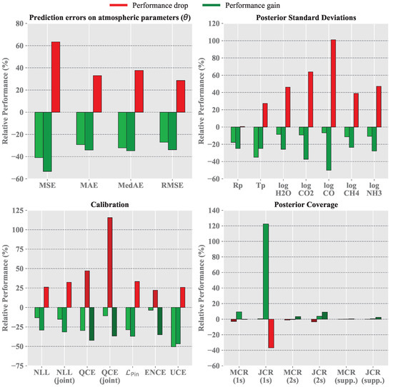
Figure 1.
Comparative analysis of model performance under the proposed posterior evaluation framework. Performance gains (positive values) and drops (negative values) are depicted in shades of green and red, respectively. From left to right, the bars show the influence of Z-score normalization over min–max scaling, noise conditioning, and realistic spectra over ideal spectra. Z-score normalization of target features and noise conditioning positively influence model performance, while the use of perturbed transmission spectra decidedly complicates the retrieval task.
First, consistent performance gains in terms of prediction error across all metrics are observed. In particular, we highlight an average reduction of about in terms of MSE measurements, and of more than for MAE, MedAE, and RMSE. Second, the Z-score normalization also shows a desirable trade-off between uncertainty estimation, calibration, and coverage. While maintaining stable posterior coverage (less than average variations as measured by MCR and JCR across multiple coverage levels), the posterior standard deviations are decidedly improved across all atmospheric parameters, either bulk parameters (average reduction of and for planetary radius and temperature, respectively) or gas abundances (varying from to average reductions). This enables more confident predictions while performing well on ground-truth benchmarking. Furthermore, Z-score normalization of atmospheric parameters provides superior calibration performance compared to target min–max scaling, in terms of sample quality (average reductions of and in terms of NLL measurements in the univariate and multivariate cases, respectively), quantile calibration (average reductions of and in terms of QCE measurements in the univariate and multivariate cases, respectively; average decrement of in terms of Pinball loss), and variance calibration (average reductions of and in terms of ENCE and UCE measurements, respectively). Notably, the superiority of Z-score normalization over min–max scaling persists even though the target features deviate significantly from a normal distribution, as demonstrated by statistical tests.
4.4. Effects of Noise Conditioning
To minimize the confounding effects of multiple variables, we consider the experimental configurations trained exclusively on ideal transmission spectra. We categorized these configurations into two groups: those employing noise conditioning and those without it, following the evaluation protocol outlined in Section 3.3. As demonstrated by the middle bars in Figure 1, our results indicate that noise conditioning significantly enhances model performance, enabling a favorable trade-off between prediction errors, uncertainty estimation, calibration, and coverage. First, it significantly reduces errors in atmospheric parameter predictions, as evidenced by improvements in MSE, MAE, MedAE, and RMSE (average reductions of , , , and , respectively). Second, it also contributes positively to uncertainty estimation, as posterior standard deviations show notable gains (average reductions varying from to ). Third, the coverage performance remains largely stable, with the exception of JCR at the level, which exhibits an average increase of 122.48%. This improvement is particularly significant, as the coverage level represents the most stringent and challenging task, while also being critical for ensuring reliable predictions. The calibration metrics reveal a more complex picture: opposing trends in quantile calibration ( and average increments in terms of QCE in univariate and multivariate cases vs. average improvement in terms of Pinball loss), as well as in terms of variance calibration ( average increment of ENCE measurements vs. average decrement of UCE measurements). We also register performance gains in terms of sample quality ( and average reductions in NLL measurements in the univariate and multivariate cases). Despite its calibration costs, noise conditioning is highly effective for tasks prioritizing prediction accuracy, uncertainty estimation, and coverage.
4.5. Robustness to Noisy Observations
We categorize all experimental configurations into those trained on realistic transmission spectra versus those trained on ideal spectra. The right-most bars in Figure 1 present the performance comparison of the former through relative percentage changes relative to the latter, quantifying the influence of realistic spectra in training and evaluation of CNFs. First of all, the use of realistic spectra leads to significant declines in atmospheric parameter predictions, with increased errors across MSE, MAE, and RMSE (average increments varying from to ). As expected, perturbed observations challenge precise parameter estimation, inducing less precise and confident predictions. In fact, similar considerations can be carried out on notable performance drops in uncertainty estimation (average increments varying from to for planet temperature and carbon monoxide log-abundance, respectively). Only the planetary radius is not marked by a performance drop in uncertainty estimation. Again, the behavior of calibration metrics is inconsistent. While quantile and variance calibration improve by registering average decrements of , , and for QCE (univariate, multivariate) and ENCE, respectively, we also register a performance drop for Pinball loss and UCE (average increment of and , respectively). Also, sample quality worsens as measured by the average increment of and of NLL measurements in the univariate and multivariate cases. Coverage metrics remain stable except for JCR at with an average decrement of . These findings highlight a reduction in robustness, with noisy observations producing qualitatively less precise predictions and poorly calibrated confidence intervals, and quantitatively reflected in increased prediction errors and reduced coverage rates.
5. Conclusions
The aim of this work is to investigate how implementation choices impact posterior robustness and predictive performance of CNFs trained with FMPE, established as a novel and scalable methodology in deep generative modeling, thus addressing a gap in the current literature. As a scientific case study, we considered atmospheric retrieval of exoplanets due to its natural need for complex simulations, and investigated the sensitivity of CNFs trained with FMPE under different modeling decisions, including data preprocessing, incorporation of input data uncertainty, and perturbed observations. We conducted an extensive experimental campaign on the ADC dataset aimed at assessing the influence of data normalization strategies, the incorporation of input data uncertainty, and the use of observations perturbed with Gaussian noise to assess robustness under controlled noise conditions. This sensitivity is particularly evident under the adopted evaluation framework, which deeply assesses complementary predictive aspects like accuracy, calibration, and uncertainty quantification, emphasizing the relevance of this study. Our analysis demonstrated the following: (i) Z-score normalization provides superior performance over min–max scaling as a target normalization strategy, independent of the evaluation task at hand. Furthermore, it enables a desirable trade-off among predictive qualities. (ii) Noise conditioning effectively improves prediction accuracy, uncertainty estimation, and posterior coverage, at the cost of calibration performance. (iii) The use of perturbed spectra strongly hinders prediction accuracy and uncertainty estimation, leading to less precise and poorly calibrated predictions and thus indicating reduced robustness under the assumed noise conditions.
Future work should expand this sensitivity analysis to a wider range of inverse problems and posterior estimators, validating our findings across domains and datasets with real observational data. In particular, examining the robustness of CNFs with FMPE under high-resolution data, such as astrophysical spectroscopy, may reveal new challenges and motivate methodological innovations to handle increased data complexity. Other promising directions include investigating the effect of alternative conditioning mechanisms or adaptations to different noise assumptions mimicking the nature of real-world data to further assess the reliability of likelihood-free inference.
Author Contributions
M.G.O.: Conceptualization, Methodology, Software, Investigation, Visualization, Writing—Original Draft. A.F.: Conceptualization, Methodology, Validation, Investigation, Writing—Review and Editing, Funding acquisition. L.I.: Conceptualization, Validation, Writing—Review and Editing. A.C.: Conceptualization, Methodology, Writing—Review and Editing. A.M.: Supervision, Writing—Review and Editing. All authors have read and agreed to the published version of the manuscript.
Funding
The authors acknowledge financial contribution from the European Union-Next Generation EU RRF M4C2 1.1 PRIN MUR 2022 project 2022CERJ49 (ESPLORA) “Finanziato dall’Unione europea-Next Generation EU, Missione 4 Componente 2 CUP Master C53D23001060006, CUP I53D23000660006”.
Data Availability Statement
The original data presented in the study are openly available in Ariel Big Challenge (ABC) Database at https://zenodo.org/records/6770103 (accessed on 8 August 2025).
Conflicts of Interest
The authors declare no conflicts of interest. The funders had no role in the design of the study; in the collection, analyses, or interpretation of data; in the writing of the manuscript; or in the decision to publish the results.
References
- Cranmer, K.; Brehmer, J.; Louppe, G. The frontier of simulation-based inference. Proc. Natl. Acad. Sci. USA 2020, 117, 30055–30062. [Google Scholar] [CrossRef] [PubMed]
- Zammit-Mangion, A.; Sainsbury-Dale, M.; Huser, R. Neural Methods for Amortized Inference. Annu. Rev. Stat. Its Appl. 2025, 12, 311–335. [Google Scholar] [CrossRef]
- Ganguly, A.; Jain, S.; Watchareeruetai, U. Amortized Variational Inference: A Systematic Review. J. Artif. Intell. Res. 2023, 78, 167–215. [Google Scholar] [CrossRef]
- Wildberger, J.B.; Dax, M.; Buchholz, S.; Green, S.R.; Macke, J.H.; Schölkopf, B. Flow Matching for Scalable Simulation-Based Inference. In Proceedings of the Thirty-Seventh Conference on Neural Information Processing Systems, New Orleans, LA, USA, 10–16 December 2023. [Google Scholar]
- Chen, R.T.Q.; Rubanova, Y.; Bettencourt, J.; Duvenaud, D.K. Neural Ordinary Differential Equations. In Proceedings of the Advances in Neural Information Processing Systems, Montréal, QC, Canada, 3–8 December 2018; Curran Associates, Inc.: Red Hook, NY, USA, 2018; Volume 31. [Google Scholar]
- Papamakarios, G.; Nalisnick, E.; Rezende, D.J.; Mohamed, S.; Lakshminarayanan, B. Normalizing flows for probabilistic modeling and inference. J. Mach. Learn. Res. 2021, 22, 57:2617–57:2680. [Google Scholar]
- Lipman, Y.; Chen, R.T.Q.; Ben-Hamu, H.; Nickel, M.; Le, M. Flow Matching for Generative Modeling. arXiv 2023, arXiv:2210.02747. [Google Scholar] [CrossRef]
- Barret, D.; Dupourqué, S. Simulation-based inference with neural posterior estimation applied to X-ray spectral fitting-Demonstration of working principles down to the Poisson regime. Astron. Astrophys. 2024, 686, A133. [Google Scholar] [CrossRef]
- Ward, D.; Cannon, P.; Beaumont, M.; Fasiolo, M.; Schmon, S.M. Robust Neural Posterior Estimation and Statistical Model Criticism. In Proceedings of the Advances in Neural Information Processing Systems, New Orleans, LA, USA, 28 November–9 December 2022. [Google Scholar]
- Fiscale, S.; Ferone, A.; Ciaramella, A.; Inno, L.; Giordano Orsini, M.; Covone, G.; Rotundi, A. Detection of Exoplanets in Transit Light Curves with Conditional Flow Matching and XGBoost. Electronics 2025, 14, 1738. [Google Scholar] [CrossRef]
- Vasist, M.; Rozet, F.; Absil, O.; Mollière, P.; Nasedkin, E.; Louppe, G. Neural posterior estimation for exoplanetary atmospheric retrieval. Astron. Astrophys. 2023, 672, A147. [Google Scholar] [CrossRef]
- Yip, K.H.; Changeat, Q.; Al-Refaie, A.; Waldmann, I.P. To Sample or Not to Sample: Retrieving Exoplanetary Spectra with Variational Inference and Normalizing Flows. Astrophys. J. 2024, 961, 30. [Google Scholar] [CrossRef]
- Gebhard, T.D.; Angerhausen, D.; Konrad, B.S.; Alei, E.; Quanz, S.P.; Schölkopf, B. Parameterizing pressure–temperature profiles of exoplanet atmospheres with neural networks. Astron. Astrophys. 2024, 681, A3. [Google Scholar] [CrossRef]
- Gebhard, T.D.; Wildberger, J.; Dax, M.; Kofler, A.; Angerhausen, D.; Quanz, S.P.; Schölkopf, B. Flow matching for atmospheric retrieval of exoplanets: Where reliability meets adaptive noise levels. Astron. Astrophys. 2025, 693, A42. [Google Scholar] [CrossRef]
- Giordano Orsini, M.; Ferone, A.; Inno, L.; Casolaro, A.; Maratea, A. Flow Matching Posterior Estimation for Simulation-based Atmospheric Retrieval of Exoplanets. IEEE Access 2025, 13, 137773–137792. [Google Scholar] [CrossRef]
- Changeat, Q.; Yip, K.H. ESA-Ariel Data Challenge NeurIPS 2022: Introduction to exo-atmospheric studies and presentation of the Atmospheric Big Challenge (ABC) Database. RAS Tech. Instruments 2023, 2, 45–61. [Google Scholar] [CrossRef]
- Sisson, S.A.; Fan, Y.; Beaumont, M. (Eds.) Handbook of Approximate Bayesian Computation; Chapman and Hall/CRC: New York, NY, USA, 2018. [Google Scholar]
- Madhusudhan, N. Exoplanetary Atmospheres: Key Insights, Challenges, and Prospects. Annu. Rev. Astron. Astrophys. 2019, 57, 617–663. [Google Scholar] [CrossRef]
- Giordano Orsini, M.; Ferone, A.; Inno, L.; Giacobbe, P.; Maratea, A.; Ciaramella, A.; Bonomo, A.S.; Rotundi, A. A data-driven approach for extracting exoplanetary atmospheric features. Astron. Comput. 2025, 52, 100964. [Google Scholar] [CrossRef]
- Hüllermeier, E.; Waegeman, W. Aleatoric and epistemic uncertainty in machine learning: An introduction to concepts and methods. Mach. Learn. 2021, 110, 457–506. [Google Scholar] [CrossRef]
- Valdenegro-Toro, M.; de Jong, I.P.; Zullich, M. Unified Uncertainties: Combining Input, Data and Model Uncertainty into a Single Formulation. arXiv 2024, arXiv:2406.18787. [Google Scholar] [CrossRef]
- Mugnai, L.V.; Al-Refaie, A.; Bocchieri, A.; Changeat, Q.; Pascale, E.; Tinetti, G. Alfnoor: Assessing the Information Content of Ariel’s Low-resolution Spectra with Planetary Population Studies. Astron. J. 2021, 162, 288. [Google Scholar] [CrossRef]
- Steinhoff, J.; Hind, S. Simulation and the reality gap: Moments in a prehistory of synthetic data. Big Data Soc. 2025, 12, 20539517241309884. [Google Scholar] [CrossRef]
- Gargaud, M.; Irvine, W.M.; Amils, R.; Claeys, P.; Cleaves, H.J.; Gerin, M.; Rouan, D.; Spohn, T.; Tirard, S.; Viso, M. (Eds.) Atmospheric Remote-Sensing Infrared Exoplanet Large-Survey. In Encyclopedia of Astrobiology; Springer: Berlin/Heidelberg, Germany, 2023; p. 275. [Google Scholar]
- Küppers, F.; Schneider, J.; Haselhoff, A. Parametric and Multivariate Uncertainty Calibration for Regression and Object Detection. In Proceedings of the Computer Vision—ECCV 2022 Workshops, Tel Aviv, Israel, 23–27 October 2022; Karlinsky, L., Michaeli, T., Nishino, K., Eds.; Springer: Cham, Switzerland, 2023; pp. 426–442. [Google Scholar]
- Yip, K.H.; Changeat, Q.; Nikolaou, N.; Morvan, M.; Edwards, B.; Waldmann, I.P.; Tinetti, G. Peeking inside the Black Box: Interpreting Deep-learning Models for Exoplanet Atmospheric Retrievals. Astron. J. 2021, 162, 195. [Google Scholar] [CrossRef]
- Aubin, M.; Cuesta-Lazaro, C.; Tregidga, E.; Viaña, J.; Garraffo, C.; Gordon, I.E.; López-Morales, M.; Hargreaves, R.J.; Makhnev, V.Y.; Drake, J.J. Simulation-Based Inference for Exoplanet Atmospheric Retrieval: Insights from Winning the Ariel Data Challenge 2023 Using Normalizing Flows. In Proceedings of the Machine Learning and Principles and Practice of Knowledge Discovery in Databases, Turin, Italy, 18–22 September 2023; Springer: Cham, Switzerland, 2025; pp. 113–131. [Google Scholar]
Disclaimer/Publisher’s Note: The statements, opinions and data contained in all publications are solely those of the individual author(s) and contributor(s) and not of MDPI and/or the editor(s). MDPI and/or the editor(s) disclaim responsibility for any injury to people or property resulting from any ideas, methods, instructions or products referred to in the content. |
© 2025 by the authors. Licensee MDPI, Basel, Switzerland. This article is an open access article distributed under the terms and conditions of the Creative Commons Attribution (CC BY) license (https://creativecommons.org/licenses/by/4.0/).