Article

A Novel Self-Recovery Fragile Watermarking Scheme Based on Convolutional Autoencoder

1
Department of Information Engineering and Computer Science, Feng Chia University, Taichung City 407102, Taiwan
2
Department of Management Information Systems, National Chung Hsing University, Taichung City 402202, Taiwan
3
Department of Information Management, Chaoyang University of Technology, Taichung City 413310, Taiwan
*
Authors to whom correspondence should be addressed.
Electronics 2025, 14(18), 3595; https://doi.org/10.3390/electronics14183595
Submission received: 12 August 2025 / Revised: 29 August 2025 / Accepted: 4 September 2025 / Published: 10 September 2025
(This article belongs to the Special Issue Digital Signal and Image Processing for Multimedia Technology)

Abstract

In the digital era where images are easily accessible, concerns about image authenticity and integrity are increasing. To address this, we propose a deep learning-based fragile watermarking method for secure image authentication and content recovery. The method utilizes bottleneck features extracted by the convolutional encoder to carry both authentication and recovery information and employs deconvolution at the decoder to reconstruct image content. Additionally, the Arnold Transform is applied to scramble feature information, effectively enhancing resistance to collage attacks. At the detection stage, block voting and morphological closing operations improve tamper localization accuracy and robustness. Experiments tested various tampering ratios, with performance evaluated by PSNR, SSIM, precision, recall, and F1-score. Experiments under varying tampering ratios demonstrate that the proposed method maintains high visual quality and achieves reliable tamper detection and recovery, even at 75% tampering. Evaluation metrics including PSNR, SSIM, precision, recall, and F1-score confirm the effectiveness and practical applicability of the method.

1. Introduction

1.1. Research Background

With rapid technological advancement, digital information has become deeply embedded in daily life. A smartphone enables us to capture special moments, preserving them as lasting digital records. The widespread use of digital imaging enables everyone to document and witness life. Meanwhile, advancements in information and communication technology (ICT) have fueled the growth of social media platforms like Facebook, Instagram, and Threads, connecting people worldwide and turning images into bridges for emotional exchange and interaction.
Beyond recording and sharing, images have become vital tools for justice. In judicial and administrative contexts, photos and videos—such as citizen recordings of crimes—serve as crucial evidence for investigation and trials. When individual rights are violated, images serve as factual evidence and offer reliable legal and social proof emphasizing their vital role in today’s world.
However, the rise of deepfake technology increasingly threatens image authenticity, producing highly realistic forged images and facial videos. Meanwhile, accessible editing tools like Microsoft Paint, Adobe software, and Canva offer users easy ways to enhance images but can also be misused to alter content maliciously, fabricating falsehoods that mislead the public and judicial systems, damaging reputations and societal trust. Since images are often regarded as factual evidence, their credibility is now under serious threat, making image integrity verification a critical topic in current research and technology.
Previous research divides image authentication methods into active and passive approaches, as shown in Figure 1 [1]. Active methods generate and store features before transmission. Common techniques include digital signatures [2], encryption [3], and watermarking [4,5,6,7,8]. The receiver compares extracted features to verify integrity. Watermarking is categorized into fragile watermarks, which detect minor changes and localize tampering, suitable for integrity verification [9,10,11,12,13]; robust watermarks, which are resistant to noise and compression, used mainly for copyright protection [10]; and semi-fragile watermarks, which balance tamper detection and resistance to common image processing [14].
Passive methods require no prior embedding and verify authenticity solely at the receiver by detecting traces left by image processing or tampering. Also called blind methods, passive approaches can be further divided based on processing domain into internal consistency and irregularity analysis, tampering detection tailored to or independent of forgery types, and handling natural images versus AI-generated images.
Compared to passive authentication, active authentication methods offer superior tamper localization capabilities. Fragile watermarks can precisely mark altered image regions, making them ideal for sensitive fields like forensic and medical imaging. Active methods also enable real-time verification by allowing receivers to compare embedded features to check image integrity. In contrast, passive authentication relies on statistical and feature analysis, which is computationally intensive, slower, and less precise in locating tampering.
In the domains of digital signatures, watermarking, and cryptography, fragile watermarking often incorporates image self-recovery technology. This not only detects tampered regions but can restore damaged parts to closely approximate the original image [15]. Such recovery capabilities significantly enhance the utility of fragile watermarking in maintaining image authenticity and preserving content integrity.

1.2. Research Motivation and Objectives

In recent years, deep learning has rapidly advanced, with convolutional neural networks (CNNs) [16] becoming a key technology in image processing. CNNs automatically learn and extract image features through hierarchical structures, offering greater adaptability and representational power than traditional handcrafted methods. Their core is the convolution operation, which uses local receptive fields and weight sharing to capture low-level features like edges and textures, and combines these into higher-level semantic information such as shapes and contours. Pooling reduces feature dimensionality, improving efficiency and translation invariance. CNNs outperform fully connected networks in generalization and classification tasks, making them central to modern deep learning architectures.
Convolutional autoencoders (CAEs) are an extension of CNNs used for feature extraction and image compression/reconstruction [17]. Composed of an encoder and decoder, the encoder applies convolution and pooling to transform input images into low-dimensional latent representations that retain essential information. These latent features are analogous to principal components in PCA, enabling data compression and improved processing efficiency.
The decoder reconstructs the image using deconvolution or up sampling to restore the features to the original size, producing a reconstruction close to the input image.
The compressed feature representations produced by the encoder can be applied to various downstream tasks [18], such as anomaly detection, image denoising, and feature learning. When combined with a decoder, these features also support extensions like super-resolution, image inpainting, and Generative Adversarial Networks (GANs) to enhance image quality and realism.
The powerful feature extraction capabilities of CNNs, combined with the compression–reconstruction structure of CAEs, make them well-suited for fragile watermarking applications that require both authentication and self-recovery. Features generated by CAEs can represent both authentication and recovery information efficiently, enhancing the watermarking scheme’s robustness and effectiveness.
While several studies have applied deep learning in fragile watermarking, most treat authentication and recovery as separate tasks handled by distinct models. This separation increases computational complexity and storage overhead. Our work addresses this gap by proposing a unified convolutional autoencoder framework that simultaneously encodes both authentication and recovery information. This integration simplifies model architecture, reduces embedding redundancy, and improves tampering detection and restoration efficiency.
Therefore, this study proposes a fragile watermarking image authentication method based on a deep learning CAE architecture. The method not only detects and localizes tampering but also autonomously recovers the tampered regions.
Section 2 reviews related work, including the block-pixel authentication method by Lee et al. [13], the SVD-based approach by Shen et al. [19], the fundamentals of CNNs and CAEs, and Rezaei’s CNN-based image recovery method [20]. Section 3 presents the proposed methodology and framework, Section 4 shows the experimental design and results, and Section 5 concludes with a summary and future directions.

2. Related Work

This Section explores existing methods and techniques proposed by researchers, including MSB, LSB, and SVD approaches. After reviewing these non-deep learning methods, we further investigate deep learning-based techniques. First, convolutional neural networks (CNNs) are introduced, followed by convolutional autoencoders. Finally, Rezaei’s CNN-based image watermark authentication method is discussed [20].

2.1. Symbol Definitions

To clearly explain the methods proposed by previous researchers, this subsection first provides complete definitions of the relevant symbols, as shown in Table 1.

2.2. Fragile Watermarking

Rakhmawati et al. [15] described the structure of fragile watermarking, as shown in Figure 2. Fragile watermarking techniques are generally categorized into two types:
(1)
Pixel-wise schemes: Extract features from individual pixels. These offer high localization accuracy but may reduce image quality due to the large amount of embedded data.
(2)
Block-wise schemes: Divide the image into non-overlapping blocks. Although this method may falsely mark some untampered pixels, it improves image quality by reducing the amount of embedded data.
In block-based schemes, the process can be divided into the following three main stages. Process 1: selection, generation, and method of watermark embedding. Process 2: detection and tamper localization. Process 3: tamper recovery.
Among these, the first stage receives the most focus, as it directly influences the effectiveness of tamper detection and recovery.
When selecting the watermark, block size (e.g., 2 × 2, 3 × 3, 4 × 4, or 8 × 8) should be considered, as different sizes affect performance and can be evaluated experimentally. Another key factor is the block-mapping sequence; improper mapping may store both authentication and recovery data in the same block, compromising tamper recovery. Common mapping techniques include Linear Transform [21,22] and Arnold Transform [23].
For watermark generation, two types of information are typically created. 1. Authentication bits to verify the integrity of each block. 2. Recovery bits to restore tampered content.
Authentication bits can be generated using hash functions or singular value decomposition (SVD) [13,19], while recovery bits are often based on block averages [13,19].
Finally, watermark embedding can be performed in either the spatial domain (e.g., Least Significant Bit, LSB) or the transform domain, using techniques such as Discrete Cosine Transform (DCT) or Discrete Wavelet Transform (DWT).

2.3. Block-Pixel Wised Image Authentication (BP Wised) and Singular Value Decomposition (SVD Based) Image Authentication

In 2019, Lee et al. proposed the block-pixel (BP) wise image authentication technique [13]. First, the image is divided into non-overlapping blocks, and each block has two parts to be processed. The first part is to calculate the authentication information A i for each block B i , while the other part is to calculate the average value of each block B i to be used as R i . The following describes the detailed process of both parts during the A i and   R i generation and embedding phases.
Step 1. Divide the original image I O into N non-overlapping blocks B i of size m × n   i = 1,2 , , N .
Step 2. Use the 6 MSBs of each block B i   to perform a hash operation to generate the authentication information A i .
Step 3. Use the average value M i of each block B i as R i .
Step 4. Use a random seed SK to generate N unique pseudo-random numbers from 1 to N , to determine which block B i   corresponds to another block B M i .
Step 5. Record R i of B i as the 8-bit average value M r m i of the corresponding block B M i .
Step 6. The watermark I W for each block B i is composed of the block’s   A i and   R i .
Step 7. Use LSB substitution to embed I W into the LSBs of block B i .
Upon receiving the tampered image I T , the receiver generates authentication codes   A i for each block B i   and compares them with the original A i . If A i = A i , the block is considered untampered; otherwise, A i A i indicates tampering.
The extracted recovery data R i , a downscaled version of the original block, is used to restore missing pixels via bicubic interpolation.
In 2020, Shen et al. proposed an SVD-based image authentication method [19], which differs from the BP-wised approach by using finer block division. This improves tampering detection accuracy, reducing both false positive and false negative rates (FPR and FNR).
The method consists of two main parts: watermark generation and embedding, and tampering detection and self-recovery, as detailed above.
The original image I O is divided into N = ( W × H ) / ( m × n ) non-overlapping blocks B i of size m × n . The average value of each block m × n is calculated to obtain the recovery data   R i .
For the authentication data A i , the two LSBs of every pixel in B i are first set to zero. Then, B i is split into four sub-blocks and combined vertically into upper and lower halves, B U i and B L i , respectively, using Equations (1) and (2). These represent the upper and lower parts of B i .
Next, singular value decomposition (SVD) is applied to B U i and B L i , yielding matrices E U i and E L i as in Equation (3). Each singular value is converted to binary, then merged via XOR operations according to Equations (4) and (5).
Finally, the binary sequences from the upper half a U and lower half a L are concatenated to form the complete authentication message A i . Both A i and   R i are embedded into the two LSBs of B i blocks, similar to the BP-wised approach.
B U i = v e r t i c a l   c o n c a t { b i 1 | | a b s b i 1 b i 2 , ( r o u n d b i 1 b i 2 2 | | b i 2 ) }
B L i = v e r t i c a l   c o n c a t { b i 3 | | a b s b i 3 b i 4 , ( r o u n d b i 3 b i 4 2 | | b i 4 ) }
E U i = a U 1 0 0 0 0 a U 2 0 0 0 0 a U 3 0 0 0 0 a U 4   a n d   E L i = a L 1 0 0 0 0 a L 2 0 0 0 0 a L 3 0 0 0 0 a L 4
a U = X O R ( a U 1 ,   a U 2 ,   a U 3 ,   a U 4 )
a L = X O R ( a L 1 ,   a L 2 ,   a L 3 ,   a L 4 )
The receiver regenerates the authentication code A i using the same method and compares it with the embedded A i stored in the two LSBs of block B i . If the first 12 bits match but the last 12 bits differ, it indicates tampering in the lower half of the block, while the upper half remains intact; the reverse applies if the first 12 bits differ and the last 12 match. If both halves differ, the entire block B i is considered unusable. Upon detecting tampering, the embedded average value is extracted and enlarged using bicubic interpolation to restore the tampered pixels.

2.4. Rezaei’s Method [20]

Rezaei et al. proposed a self-recovery framework using CNNs, where authentication and recovery bits are processed by different networks. Authentication uses a fine-tuned VGG-16 model, while recovery employs the CNN-based compression network by Feng et al. [24]. The following sections describe (1) watermark generation and embedding, and (2) image tampering detection and recovery.
The watermark A i is generated by fine-tuning a VGG-16 model. The input to the model is a 16 × 16 block B i , with its two least significant bits (LSBs) removed to reserve space for embedding A i and recovery data R i . The fine-tuned VGG-16 outputs a 16-element vector, with each value quantized to 8 bits.
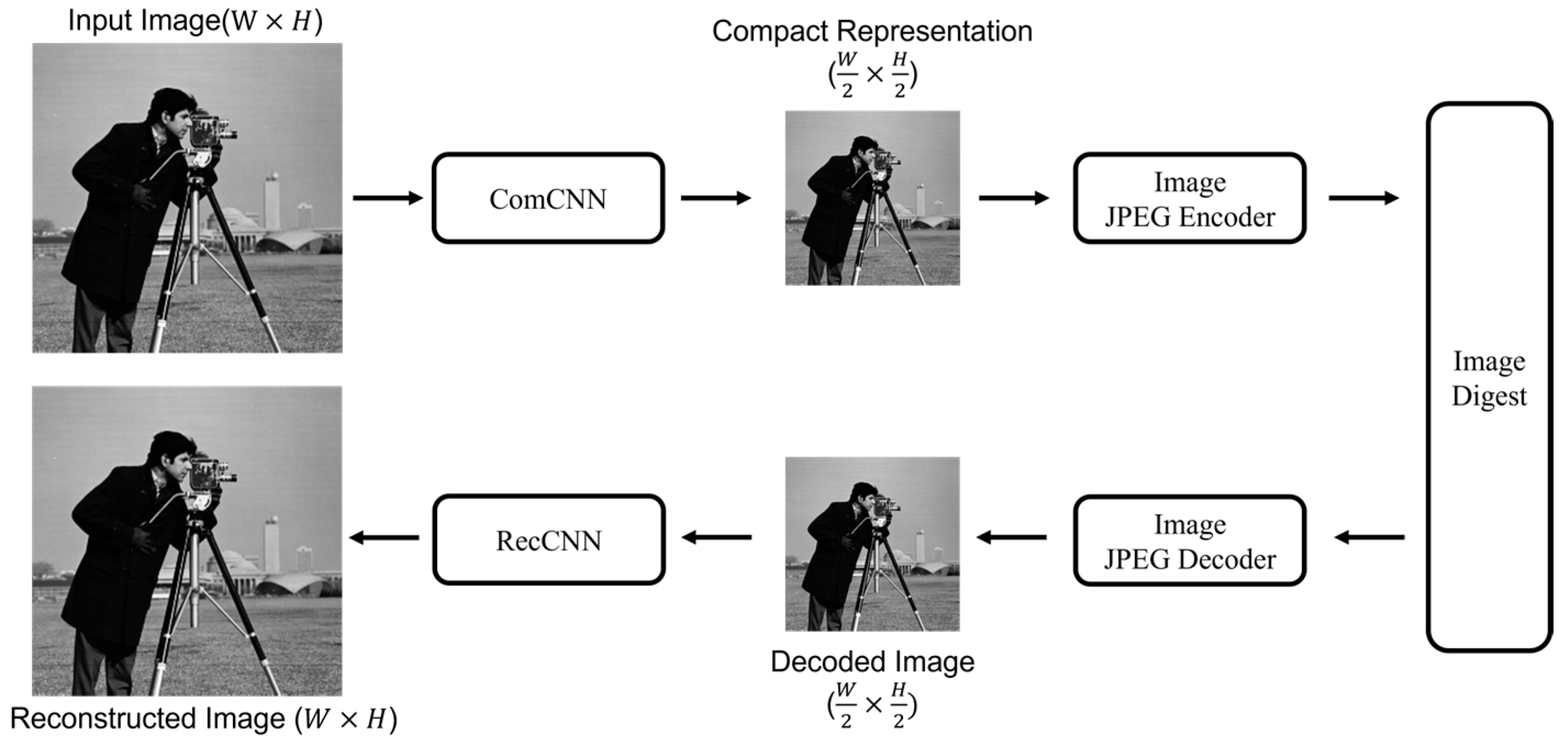
The recovery data R i generation follows the approach proposed by Feng et al., as illustrated in Figure 3.
As ComCNN and RecCNN serve as the compression and decompression networks, respectively, both are designed based on convolutional neural networks (CNNs). ComCNN compresses the original image of size ( W × H ) into a reduced version of ( W / 2 × H / 2 ) using convolutional operations. The image is then passed through a standard JPEG encoder and decoder, simulating traditional compression and decompression techniques.
The output from the JPEG encoder is organized in a zigzag scanning order, from which the first 10 coefficients are extracted. Each of these values is represented using 6 bits. These 10 coefficients are then encoded using Reed–Solomon (RS) codes for error correction, enabling recovery in case of tampering or data corruption.
To enhance security and resistance to collage attacks, the encoded data undergoes a structured scrambling process using the Arnold Transform. Finally, both the scrambled authentication data A i and recovery data R i are embedded into the two least significant bits (LSBs) of the output image I O   using a 2-LSB embedding technique.
In the second stage, tampering detection and recovery are performed. The receiver first uses a fine-tuned VGG-16 model to regenerate the authentication code   A i . This regenerated code is then compared with the embedded   A i , which was stored in the two least significant bits (LSBs) of each block. If A matches A i , the corresponding block   B i is considered untampered. Otherwise, a mismatch indicates that   B i has been tampered with.
When tampering is detected, the embedded recovery data R i , also stored in the 2 LSBs, is used to reconstruct the affected block. As shown in the lower part of Figure 3, the recovery process begins by applying inverse JPEG operations on R i , generating a low-resolution image of size ( W / 2 × H / 2 ) . This image is then processed using RecCNN with transposed convolution to upscale and restore a high-resolution approximation of the original block B i . The restored block is finally inserted back into the tampered region, completing the image recovery.
In summary, while BP-wised and SVD-based approaches offer simple designs and reasonable performance, they rely heavily on handcrafted features and bicubic interpolation, which may not generalize well under complex attacks. Rezaei’s method improves performance using deep learning but requires separate networks for different tasks, increasing system complexity. In contrast, our CAE-based method unifies feature embedding and recovery, offering a more compact, efficient, and effective solution for robust image authentication and restoration. Recent contributions further advance this direction. Dual watermarking methods for copyright protection and authentication [25], comprehensive surveys of deep learning-based watermarking challenges and future trends [26], and latent space steganographic embedding via autoencoders [27] highlight the evolution toward more robust and efficient watermarking frameworks. The following section introduces our proposed CAE-based fragile watermarking and self-recovery scheme.

3. Proposed Method

Fragile watermarking is an effective technique for ensuring image integrity, supporting not only tamper detection and localization but also recovery. To enhance restoration quality and leverage the strength of deep learning in feature extraction, this study proposes a fragile watermarking method based on a convolutional autoencoder (CAE).
The approach uses the CAE encoder to extract latent space features—high-level compact representations of the image, referred to as bottleneck information. In this context, the bottleneck denotes the compressed latent representation at the center of the CAE, where redundant details are discarded, and only essential semantic and structural features are preserved for tamper detection and recovery. Specifically, compared to the original CAE model, we reduced the number of convolutional filters in each layer, employed fewer downsampling operations, and adopted a bottleneck size of 64 instead of larger latent dimensions. These modifications were made to strike a balance between feature richness and computational efficiency. The simplification reduces parameter count and training time, while still retaining sufficient representational power for tamper detection and recovery. As a result, the proposed model achieves competitive accuracy with significantly lower computational cost compared to deeper or more complex CNN-based restoration frameworks. In terms of computational complexity, the proposed lightweight CAE has approximately O(n·k2) operations per layer, where n denotes the number of feature maps and k the kernel size, which is considerably lower than deeper CNN-based methods. On an NVIDIA GeForce 396 GTX 1650 GPU, training required about 12 h for 40,000 images, while inference for a single 256 × 256 image averaged 0.048 s. This demonstrates that the model is efficient enough for near real-time tamper detection and recovery. These features are embedded into non-overlapping image blocks. Before embedding, a random sequence generated from a secret key determines the number of Arnold Transform scrambling iterations per block, helping resist collage attacks.
The previous CAE-based or dual network methods, which often require separate modules for authentication and recovery, our strategy embeds a single compact bottleneck representation that supports both simultaneously. This shared embedding not only reduces computational overhead but also enhances robustness by ensuring that tamper detection and recovery are jointly optimized. The integration of Arnold scrambling and block-wise voting further strengthens security against collage attacks and localized tampering, making our approach more resilient than conventional methods.
At the receiver side, the embedded information is extracted and descrambled. A voting mechanism selects the most frequent bottleneck as the correct one, which is then decoded to reconstruct the image. Tampered blocks are replaced with restored versions, while untampered blocks remain unchanged, resulting in a fully recovered image.
This two-stage process is visually demonstrated in Section 4.4.2. These figures illustrate the progression from initial detection (Step1) to refined reconstruction (Step2), showing significant improvement in the clarity and accuracy of the restored images.
The full process is detailed in Section 3.1 and Section 3.2, with corresponding flowcharts provided in the following Figure 4.

3.1. Watermark Generation and Embedding

3.1.1. Encoder and Bottleneck

As shown in Figure 4, the watermark generation and embedding process begins by using an encoder to produce the bottleneck representation. The encoder is designed to align with the decoder used for tamper localization and self-recovery.
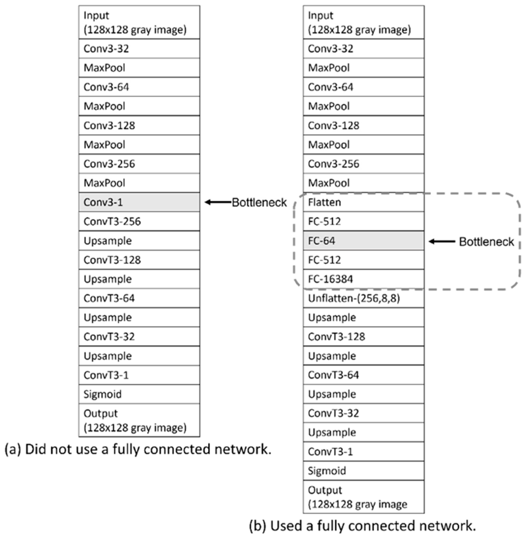
The model architecture is inspired by the VGG11 network [28] but is simplified to fit our specific task. Unlike the original VGG11, which is built for large-scale classification across 1000 categories, our model does not require such complexity. The streamlined architecture of our encoder is illustrated in Figure 5.
The model takes a grayscale image of size W × H as input, which is first converted into a tensor for efficient GPU computation. The image then passes through multiple convolutional layers, each using a 3 × 3 kernel—consistent with the VGG11 architecture. The number of channels is controlled by a variable t, as detailed in Section 4. Each convolutional layer is followed by batch normalization and a Rectified Linear Unit (ReLU) activation to stabilize training and model non-linear relationships. Downsampling is performed using pooling layers after certain convolutions. The resulting feature maps are flattened into a 2048-dimensional vector and passed through a fully connected layer to generate a 64-dimensional bottleneck vector V. This vector is then quantized so that each element is represented using 8 bits. The bottleneck size of 64 was chosen to balance between high-quality reconstruction and sufficient spatial redundancy for tamper localization. As shown in Section 4.3.6, it provides optimal performance (PSNR > 29.2 dB, SSIM > 0.92) without sacrificing localization accuracy.

3.1.2. Multiple Copies

In the watermark generation and embedding process, multiple copies of the Bottleneck are created to ensure image quality can still be restored even under heavy tampering. This redundancy not only improves recovery performance but also enables effective tampering localization.
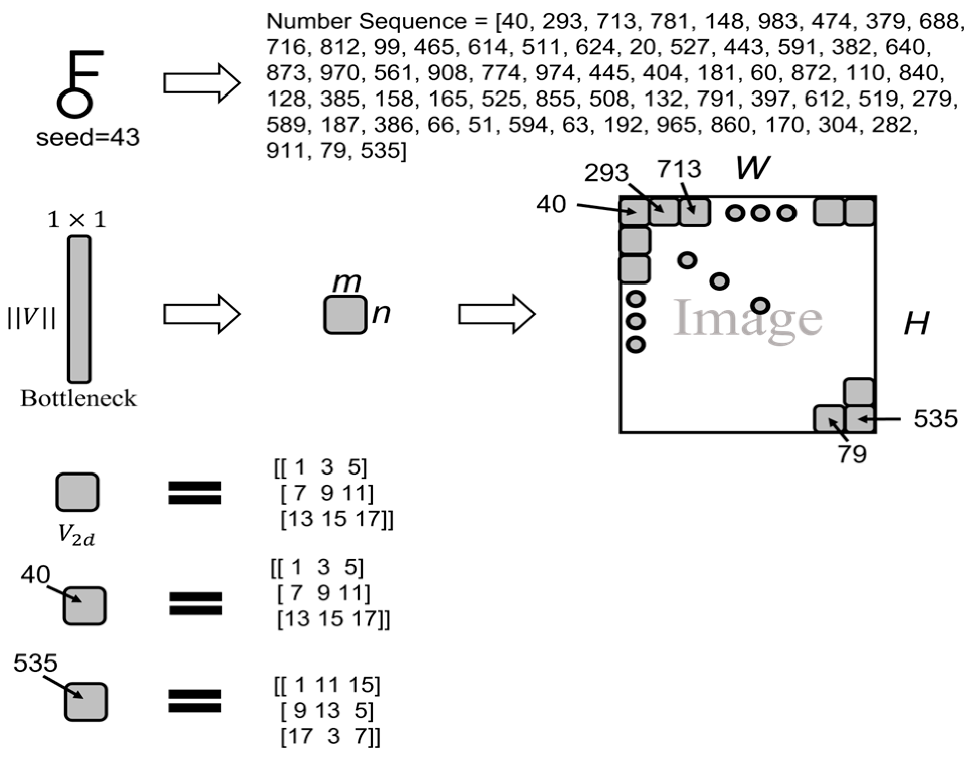
Given an original image I O of size W × H , the Bottleneck vector V is duplicated N times, where N = W × H / ( m × n ) . The vector is then reshaped into a 2D matrix, denoted as V 2 d , to fill the entire image I O , as illustrated in Figure 6.

3.1.3. Number Sequence and Scrambling

The generation of the pseudo-random sequence and scrambling process consists of two steps:
First, a random seed (secret key) is used to generate N pseudo-random numbers, where N = ( W × H ) / ( m × n ) . The numbers are produced using the Mersenne Twister algorithm, each a unique integer between 1 and 1000.
Next, the Bottleneck is scrambled using the Arnold Transform, commonly applied in image encryption by rearranging matrix positions to achieve encryption. The Arnold Transform matrix is shown in Equation (6), where ( x , y ) represents the original coordinates in the 2D Bottleneck matrix V 2 d   , x ,   y are the transformed coordinates after scrambling, and v is the matrix dimension. The modulo v ensures the transformed coordinates remain within matrix bounds.
x y = 1 1 1 2 T × x y   m o d   v
The numbers in the number sequence generated by the secret key represent the number of times T the Arnold Transform is applied. This scrambling introduces spatial diversity in otherwise identical bottleneck vectors. By applying T iterations of transformation based on a pseudo-random sequence, the method ensures that the same data appears differently across blocks, making it difficult for attackers to perform a successful collage attack using regions from the same or other watermarked images. A higher T increases the randomness and thus enhances tamper resistance. Since the pseudo-random sequence is generated using a 32-bit key, the probability of key collisions across images is negligible in practice. We considered robustness against intentional attacks. Adaptive adversarial perturbations may attempt to degrade detection, while forgery-aware scrambling reversal could exploit partial knowledge of the transform. However, block-wise pseudo-random scrambling makes reversal computationally infeasible, even with partial knowledge. Finally, although using a unique key per image strengthens security, it also introduces usability challenges. Future work will explore hierarchical or session-based key management to balance robustness and practicality. The corresponding illustration is shown in Figure 7, where V 2 d is a hypothetical value. We apply scrambling from 40 times at the top-left block up to 535 times at the bottom-right block.

3.2. Tampering Localization and Self-Recovery

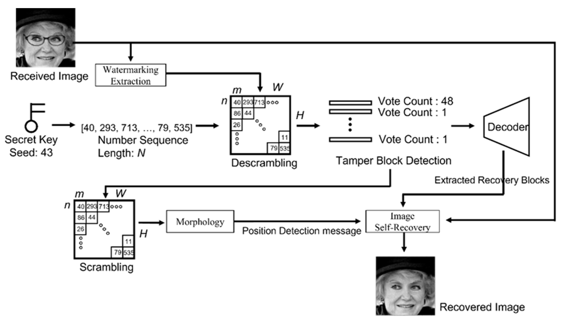
As illustrated in Figure 8, the tampering localization and self-recovery process begins by extracting the embedded scrambled bottleneck information from each block. Using the same random seed, a consistent number sequence is regenerated to descramble each block’s bottleneck using the inverse Arnold matrix. The most frequently occurring bottleneck across all blocks is identified as the correct value, while differing values are marked as tampered blocks. Since the sequence is restored before statistical analysis, the tampering map corresponds to the original positions. Morphological closing is then applied to improve detection accuracy. Finally, the correct bottlenecks are decoded and merged with untampered blocks to produce the final recovered image.

3.2.1. Watermarking Extraction, Number Sequence, and Descrambling

Watermark extraction involves retrieving information from each block using two LSBs, while generating a number sequence with the same key, as shown in Figure 9. The descrambling process restores the scrambled bottleneck values by applying the inverse Arnold Transform. The number sequence determines the number of inverse iterations, T. The inverse Arnold Transform is given in Equation (7), where x ,   y are the 2D coordinates of the extracted bottleneck block and x , y are the original coordinates obtained by the inverse operation. Here, v represents the bottleneck’s side length, and the modulo v ensures the coordinates remain within valid bounds.
x y = 2 1 1 1 T × x y m o d   v

3.2.2. Tamper Block Detection (Vote), Scrambling, and Morphology

After extracting and descrambling the bottleneck values of each block, we perform a statistical voting process to locate tampered regions, as illustrated in the tampering detection voting flow in Figure 10. However, to accurately pinpoint tampering locations, a second scrambling operation is necessary because the current voting is based on descrambled data.
Next, morphological image processing is applied to address potential False Negatives—cases where extracted LSBs are identical but the actual pixel values differ—allowing for correction of missed tampering detections.

3.2.3. Decoder and Image Self-Recovery

After determining the most reliable bottleneck, it is fed into the decoder to reconstruct an image of the same size as the original. The decoder design in Figure 5 mirrors the encoder structure: the bottleneck is first expanded to 2048 dimensions via a fully connected layer, reshaped into two dimensions, then processed through multiple upsampling and transposed convolution layers. Upsampling uses bilinear interpolation at twice the original size, while transposed convolutions incorporate batch normalization and ReLU activation to enhance feature learning and training stability. The final output layer employs a Sigmoid activation to ensure the output image values lie within [0, 1], facilitating tensor operations and loss computation.
We designed a combined loss function integrating Structural Similarity Index (SSIM) and Root Mean Square Error (RMSE) to comprehensively evaluate the quality of images generated by the autoencoder. SSIM, a statistical metric assessing similarity in structure, luminance, and contrast [29], is formulated as in Equation (8). This loss balances structural features with pixel-level accuracy for improved reconstruction quality.
In this study, X and   Y represent the input and target images, respectively. μ X and   μ Y denote local means, σ X 2   and σ Y 2   are local variances, σ X Y is the covariance, and C 1 and C 2   are constants for numerical stability. We estimate these local statistics using a Gaussian blur with a 3 × 3 window. Since SSIM is a similarity metric ranging from [−1, 1] with an ideal value of 1, we convert it into a loss function by subtracting SSIM from 1, defining the SSIM loss as in Equation (9).
RMSE measures pixel-wise error between images, calculated as shown in Equation (10), where W × H   is the number of pixels, and X i , Y i are the predicted and target pixel values. Lower RMSE indicates closer pixel-level similarity, making it suitable as a loss function defined in Equation (11).
To balance structural similarity and pixel-wise accuracy, we propose a combined SSIM–RMSE loss function weighted by α and β , as formulated in Equation (12).
S S I M X , Y = ( 2 μ X μ Y + C 1 ) ( 2 σ X Y + C 2 ) ( μ X 2 + μ Y 2 + C 1 ) ( σ X 2 + σ Y 2 + C 2 )
L S S I M = 1 S S I M ( X , Y )
R M S E X , Y = 1 W × H i = 1 W × H ( X i Y i ) 2
L R M S E = R M S E X , Y
L t o t a l = α L S S I M + β L R M S E
Finally, image self-recovery performs the final processing by combining the tampering localization information, recovery data, and the received image. First, it identifies which blocks have been tampered with and were not based on the localization results. For the tampered regions, the corresponding blocks from the recovery data are used for restoration, while untampered regions retain the blocks from the received image. This approach is adopted because, although untampered blocks contain watermarks, their image quality is generally better than that of the recovered blocks. By integrating these three sources of information, the method achieves the best possible image restoration.

4. Experimental Results

4.1. Experiment Environment and Dataset

The experiments were conducted using Python version 3.11, with the PyTorch 2.1.0 deep learning framework and GPU acceleration enabled via CUDA. The computing environment consisted of a 12th-generation Intel® Core™ i7-12700F CPU, an NVIDIA GeForce GTX 1650 GPU, 48 GB of RAM, and a 64-bit Windows 10 operating system.
This study utilized the CelebFaces Attributes Dataset (CelebA) [30], containing 202,599 celebrity face images across 10,177 identities with 40 facial attributes (e.g., gender, age, expression). Following CelebA’s original split, images are divided into training (1–162,770), validation (162,771–182,637), and testing (182,638–202,599) sets to avoid identity overlap. We randomly selected 40,000 training images to train the convolutional autoencoder and 10,000 testing images for model evaluation and fragile watermark experiments. However, since CelebA consists solely of aligned facial images, the diversity of textures and structures is limited. This may constrain the generalizability of our model to other image types such as natural scenes, documents, or medical images. In future work, we plan to evaluate the proposed method on more diverse datasets to confirm its broader applicability.
During preprocessing, the original JPG images were first converted to PNG format to enable watermark embedding. Images were then converted to grayscale, and center-cropped to a fixed resolution of 128 × 128 pixels. If the original image dimensions were insufficient, black padding was applied to maintain uniformity. The grayscale conversion emphasized the green channel’s luminance aligned with human visual perception—rather than computing a simple RGB average, as defined in Equation (13) [31].
G r a y = 0.299 × R + 0.587 × G + 0.114 × B
Figure 11 shows examples of our processed images, each sized 128 × 128 pixels, with their names displayed below. In the experimental design, these 128 × 128 images are divided into non-overlapping blocks of 16 × 16 pixels.

4.2. Evaluation Metrics

To evaluate the quality of image processing, such as watermark embedding or tampering recovery, we use two common metrics: Peak Signal-to-Noise Ratio (PSNR) and Structural Similarity Index (SSIM). PSNR measures signal fidelity, while SSIM focuses on structural and perceptual quality [30].
For tampering recovery assessment, we apply two approaches: a full-image evaluation to quantify overall quality changes, and a focused analysis on tampered regions to detail recovery performance, with comprehensive results recorded.
PSNR is calculated as in Equation (14), where higher values indicate greater similarity. L represents the maximum pixel value (255 for 8-bit images). Mean Squared Error (MSE), defined in Equation (15), measures the average squared difference between pixels X i and Y i of the original and processed images, with image dimensions W × H . Lower MSE leads to higher PSNR, reflecting smaller differences between images.
P S N R = 10 × l o g 10 ( L 2 M S E )
M S E = 1 W × H i = 1 W × H ( X i Y i ) 2
The SSIM calculation is defined in Equation (16), where μ X and μ Y denote the mean luminance of the original image X and processed image Y, respectively. σ X 2 and σ Y 2 represent the variances of the images, measuring contrast. σ X Y is the covariance between the two images, indicating their similarity. C 1 and   C 2 are stability constants.
S S I M X , Y = ( 2 μ X μ Y + C 1 ) ( 2 σ X Y + C 2 ) ( μ X 2 + μ Y 2 + C 1 ) ( σ X 2 + σ Y 2 + C 2 )
Following the image quality evaluation, we introduce recall, precision, and F1-score as metrics for tampering localization. These are calculated using True Positives (TP), False Positives (FP), True Negatives (TN), and False Negatives (FN), with formulas given in Equations (17) and (18).
R e c a l l = T P T P + F N
P r e c i s i o n = T P T P + F P
Recall and precision range from 0 to 1. Recall measures the proportion of actual tampered samples correctly identified, reflecting the model’s detection capability. Precision indicates the proportion of predicted tampered samples that are truly tampered, reflecting prediction accuracy. To balance both, the F1-score is used as a comprehensive metric—defined as the harmonic mean of precision and recall Equation (19)—suitable for scenarios requiring both accuracy and completeness.
F 1 = 2 × P r e c i s i o n × R e c a l l P r e c i s i o n + R e c a l l

4.3. Comparison of Convolutional Autoencoders with Different Parameters

The convolutional autoencoder in this study is inspired by the VGG11 architecture. Since VGG11 was originally designed for ImageNet classification, its structure is relatively complex. However, this research focuses on image compression and reconstruction, which does not require such a large model. Therefore, VGG11 was simplified and adapted to better suit the needs of an autoencoder.

4.3.1. Need for Fully Connected Layer Design

This consideration stems from the question of whether flattening is necessary in convolutional networks. The network design comparison is illustrated in Figure 12.
Figure 12a shows the architecture without fully connected layers, where the bottleneck retains a 2D shape of (8, 8). In contrast, Figure 12b introduces fully connected layers by flattening the feature map and reducing its dimensions sequentially to 512 and then 64 to form the bottleneck. Both architectures apply ReLU after convolutional and fully connected layers, and the bottleneck is quantized to 8-bit values within the range of 0–255.
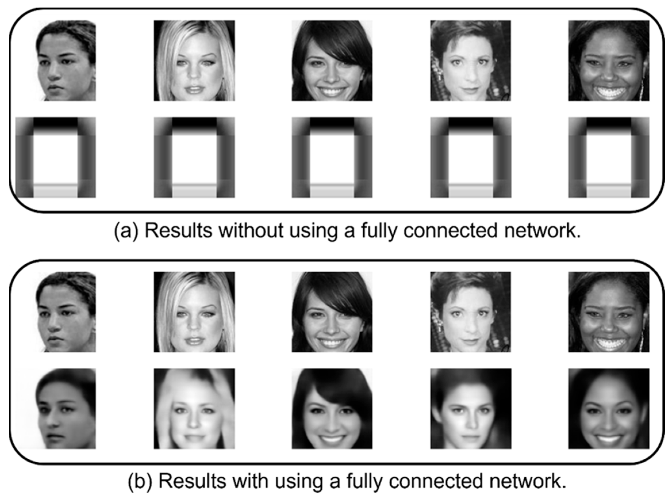
This comparison aims to evaluate whether preserving a 2D structure benefits reconstruction. However, implementation results demonstrate that using fully connected layers significantly improves reconstruction quality. As shown in Figure 13, both models were trained on 40,000 images and tested on 10,000. Figure 13a, without fully connected layers, shows inferior results, while Figure 13b illustrates noticeable improvement with them.

4.3.2. Adjustment of Network Scale

We evaluated the impact of varying network depths on image compression and reconstruction quality to determine the optimal architecture. The tested models followed a fully connected encoder–decoder design, as described in Section 4.3.1, using ReLU activation and 3 × 3 kernels for all convolutional and deconvolutional layers. Downsampling and upsampling were handled using MaxPooling and upsampling layers, respectively. The results, summarized in Table 2, show how deeper networks improve performance up to a certain point before diminishing returns appear.
The best performance was achieved using the configuration of model architecture (c), trained on 40,000 images and evaluated on a test set of 10,000 images. As shown in Table 2, this setup yielded the highest average PSNR of 28.583 dB and an SSIM of 0.850.

4.3.3. Batch Normalization

This subsection explores the impact of adding batch normalization to the model originally described in Section 4.3.1. In the modified architecture, batch normalization layers were introduced before each ReLU activation following the convolutional layers. This adjustment aimed to improve convergence and stability during training. The performance comparison between the original and modified models is summarized in the results, demonstrating improved reconstruction quality with the inclusion of batch normalization.
As shown in the implementation results in Table 3, applying batch normalization yields better performance compared to models without it.

4.3.4. Effect of Dropout

To investigate whether dropout could improve reconstruction performance and reduce overfitting, we experimented with dropout rates of 0%, 5%, 10%, and 20% in the fully connected layers. However, the results showed minimal or even slightly negative impact on image quality. Therefore, dropout was excluded from the final model configuration.

4.3.5. Loss Function Weight

We evaluated the effect of different weight combinations for the SSIM and RMSE components in our loss function. Among the tested settings, assigning a higher weight to SSIM (e.g., 0.8 SSIM, 0.2 RMSE) yielded the best balance between structural fidelity and pixel-wise accuracy. As a result, this weighting scheme was adopted for the final model.

4.3.6. Variation in the Number of Bottlenecks

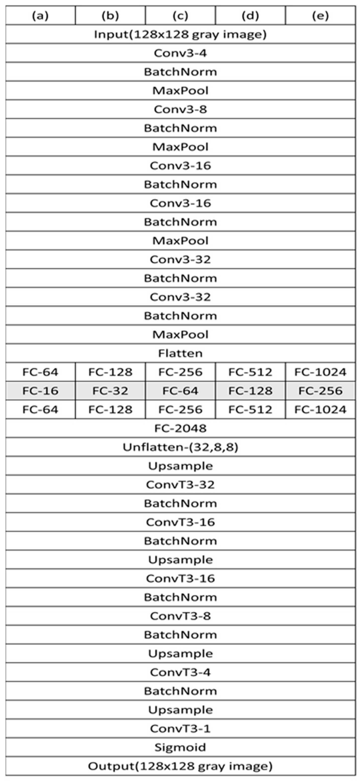
This subsection investigates the impact of bottleneck vector size on image reconstruction quality. Experiments use the previously described architecture: four layers with fully connected layers, no dropout, batch normalization enabled, and a loss function weighted 0.8 for SSIM and 0.2 for RMSE. As shown in Figure 14, the number of bottlenecks increases from 16 to 256 (Figure 14a–e). Results summarized in Table 4, based on 40,000 training and 10,000 testing images, indicate that larger bottlenecks improve reconstruction quality but reduce tampering localization accuracy due to fewer voting blocks [13,19,20]. Therefore, a compromise of 64 bottlenecks is adopted.
Based on extensive experiments comparing factors such as the use of fully connected layers, network size, and batch normalization, we finalized the number of encoder bottlenecks at 64. When correctly extracting these bottlenecks for reconstruction, the restored images achieve an average minimum quality of PSNR 29.297 dB and SSIM 0.921.

4.4. Tampering Recovery Results Under Different Scenarios

This section analyzes experimental results under watermark embedding and various tampering scenarios. Section 4.4.1 evaluates the impact of watermark embedding on image quality using PSNR and SSIM compared to the original images. Section 4.4.2 assesses tampering localization performance through recall, precision, and F1-score, alongside PSNR and SSIM metrics for both the overall and tampered regions in restored images. Section 4.4.3 further examines statistical results across different tampering ratios.

4.4.1. Watermarked Image Quality

Table 5 presents the results of embedding 64 compressed 8-bit messages—obtained via the encoder—into 128 × 128 images by replicating them across 16 × 16 blocks. The data represent averages over 10,000 test images and are comparable to prior studies employing dual LSB embedding methods [13,19,20]. Across the 10,000 test images, the average PSNR and SSIM after watermark embedding were 43.654 dB and 0.999, respectively, indicating negligible quality degradation.

4.4.2. Tampering Methods in Different Scenarios

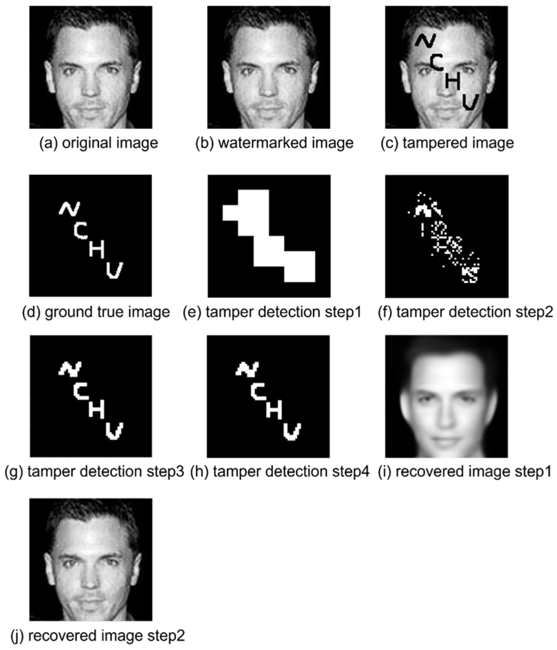
Figure 15 illustrates the complete processing pipeline of the proposed model in addressing eyeglass tampering attacks. Figure 15a presents the original input image, while 15b shows the watermarked version, which achieves a PSNR of 43.85 dB and an SSIM of 1.0. In Figure 15c, tampering is introduced using Photoshop by adding eyeglasses. Comparing Figure 15c with Figure 15b yields the tampering map in Figure 15d, revealing a tampered region covering 6.86% of the image. In the first stage of tamper detection, illustrated in Figure 15e, all bottleneck features are extracted and descrambled. A voting mechanism is then applied to detect suspicious 16 × 16 blocks with low vote frequency. Figure 15f further refines these regions by pinpointing tampered 2 × 2 sub-blocks. These refined tampering details are then scrambled back to their original positions in Figure 15g, followed by morphological closing in Figure 15h to enhance localization. The final detection achieves a recall of 0.994, precision of 0.829, and F1-score of 0. 904. Figure 15i displays the reconstructed image generated from the decoded bottleneck features. In Figure 15j, the final restored image is created by combining information from Figure 15c,h,i: untouched regions retain the original pixels from Figure 15c, while tampered regions are replaced by reconstructed content from Figure 15i. The overall restored image reaches a PSNR of 38.745 dB and SSIM of 0.994. Specifically, the restored tampered region achieves a PSNR of 29.281 dB and an SSIM of 0.743.
Figure 16 illustrates the processing of graffiti-like text tampering. Figure 16a is the original image, and Figure 16b is the watermarked version with PSNR 44.096 dB and SSIM 1. In Figure 16c, “NCHU” text is added on the face using MS Paint. Figure 16d shows the ground truth tampering mask (3.229% tampered). Figure 16e extracts bottleneck features, performs descrambling, and uses voting to detect anomalous blocks. Figure 16f refines pixel-level anomalies, followed by scrambling to restore positions, shown in Figure 16g. Figure 16h applies morphological closing for enhanced detection: recall 1.0, precision 0.722, and F1-score 0.839. Figure 16i is the decoder output using the most-voted bottleneck, and Figure 16j is the final recovery—keeping Figure 16c’s pixels for untampered regions and using Figure 16i for tampered areas. Final image recovery: PSNR 40.748 dB, SSIM 0.999; tampered region: PSNR 29.707 dB, SSIM 0.921.
A more specific form of tampering is the collage attack, where one watermarked image is used to tamper with another. As shown in Figure 17a,b are watermarked images with keys 42 and 43, respectively. In Figure 17c, the face from Figure 17b is pasted onto Figure 17a using Photoshop, creating a tampered image. Figure 17d shows the ground truth tampering mask, with a tampering ratio of 31.104%.
The detection and recovery process (Figure 17e–j) follows the same steps as in standard tampering. The localization result Figure 17h achieves recall 0.995, precision 0.929, and F1-score 0.961. The final recovered image Figure 17j has a PSNR of 33.967 dB and SSIM of 0.991 overall; within the tampered region, PSNR is 29.52 dB and SSIM is 0.853.

4.4.3. Analysis of Different Tampering Levels

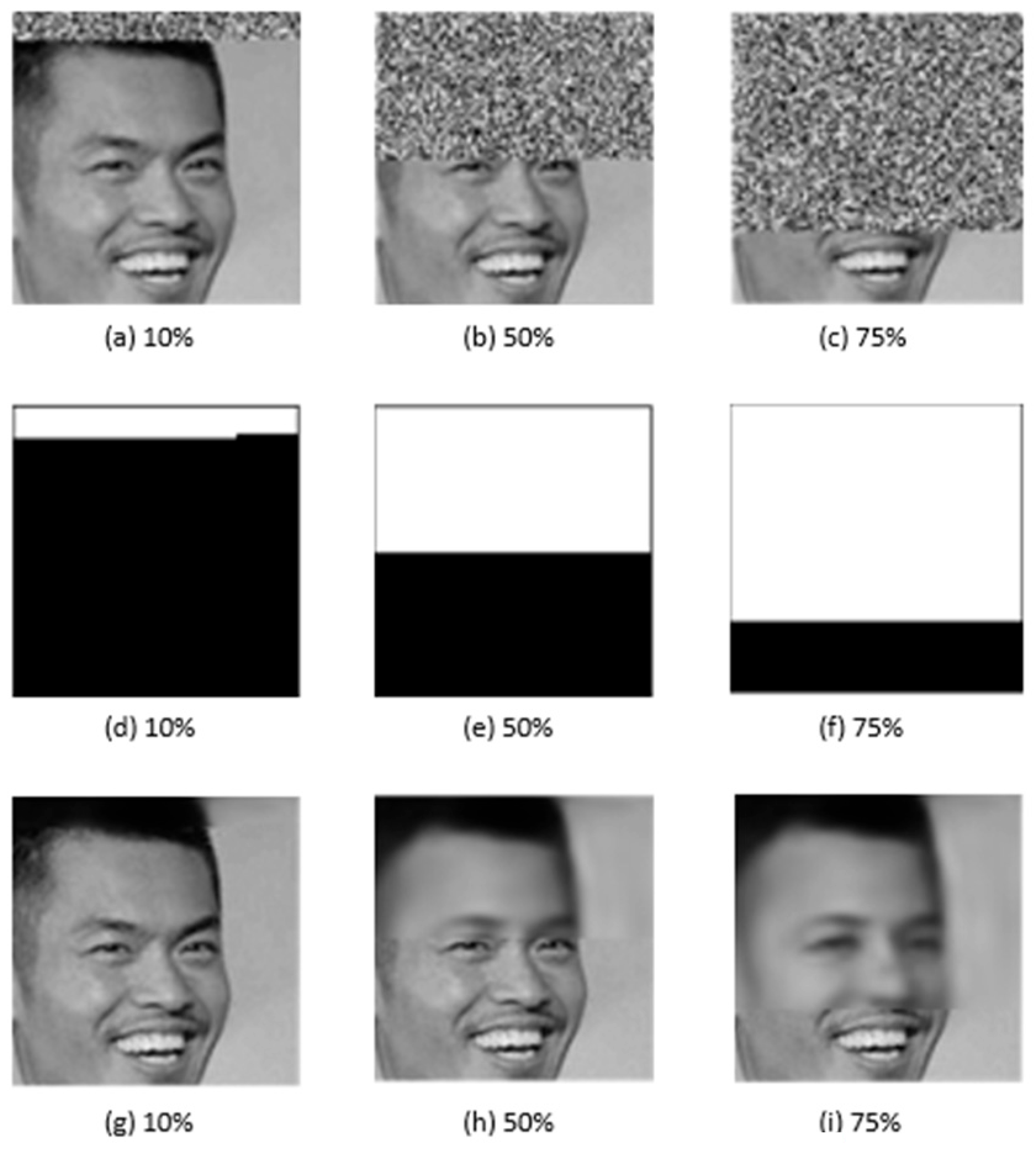
To visually demonstrate the performance of the proposed watermarking method, we selected three representative tampering levels: 10%, 50%, and 75%. As illustrated in Figure 18, the top row displays the tampered images, the middle row shows the tampering localization (binary masks), and the bottom row shows the corresponding recovered outputs.
At low tampering levels (10%), the model produces high-fidelity recovery with minimal visual artifacts. At moderate (50%) and severe (75%) tampering, the detection remains accurate, and the self-recovery performance maintains structural consistency. Despite some blurring at higher tampering rates, facial features and contextual information are largely preserved. However, certain high-frequency regions, such as eyes and lips, tend to lose sharpness due to the smoothing nature of convolutional autoencoders. This reflects a common limitation of CAE-based reconstruction. Future work may explore incorporating attention mechanisms or GANs to improve perceptual quality while maintaining tamper detection accuracy.
Table 6 summarizes recovery statistics for entire images, averaged over 10,000 test images. Table 7 presents recovery statistics for tampered regions, also averaged over 10,000 images. Table 8 reports the average recall, precision, and F1-Score for different tampering levels on the test set.
In addition to basic tampering, we evaluated the model’s robustness under collage attacks, which simulate highly inconsistent and non-uniform tampering scenarios. Figure 19 presents qualitative results at three tampering levels: 10%, 40%, and 75%. The first row displays tampered images with patches from foreign sources. The second row shows the tampering detection results, where the model successfully localizes irregular regions. The third row presents the recovered images, where even under severe 75% tampering, the method manages to reconstruct face structure with acceptable visual quality.
These results confirm the method’s strong tampering localization and recovery capabilities in the presence of complex attacks.
Table 9 presents the average overall recovery quality of 10,000 images after collage attacks at different tampering levels. Table 10 shows the average recovery quality within tampered regions. Table 11 summarizes the average detection metrics (recall, precision, F1-Score) across tampering levels.

4.5. Comparison of Our Method with Other Researchers’ Methods

This section compares our method with BP-wised [13], SVD-based [19], and Rezaei et al. [20]. Table 12 shows watermark image quality results. Our method, BP-wised, and SVD-based averaged over 10,000 CelebA test images, while Rezaei et al. used the BOWS2 dataset, with data cited from [20].
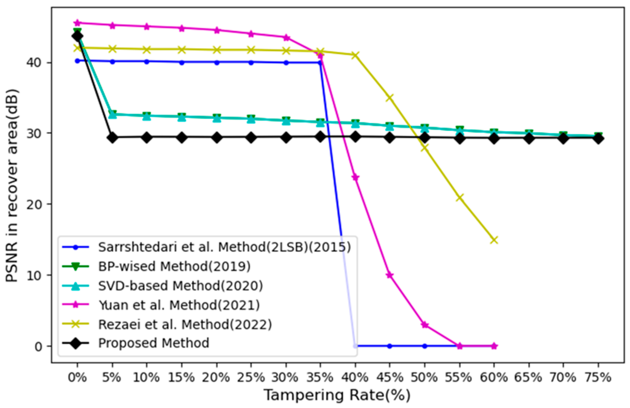
As illustrated in Figure 20, our method demonstrates superior restoration performance, particularly under high tampering rates.
Experiments show minimal difference between our method and others in terms of average PSNR at low tampering levels, as all embedded watermarks in the 2 LSBs. For fair evaluation, our method, BP-wised, and SVD-based approaches averaged results over 10,000 CelebA test images, while Rezaei et al. reported results on a single grayscale Cameraman image, from [20].
Our method excels at higher tampering ratios by leveraging accurate bottleneck information extracted from the convolutional autoencoder. Although BP-wised and SVD-based techniques sustain decent PSNR under heavy tampering due to intact verification data and bicubic interpolation, they achieve relatively lower SSIM values. This highlights our model’s strength in both structural fidelity and pixel-wise recovery accuracy under severe attack conditions.
SSIM was used to evaluate recovery in tampered regions at different tampering levels. Our method, BP-wised, and SVD-based used the CelebA test set, while Rezaei et al. used the BOWS2 dataset; results are shown in Figure 21 and referenced from [20].
Experiments show that above 60% tampering, our method outperforms others due to deep learning’s ability to preserve image structure and improve SSIM. At low tampering levels, concentrated edge tampering and limited morphological effects increase noise sensitivity, resulting in lower SSIM.
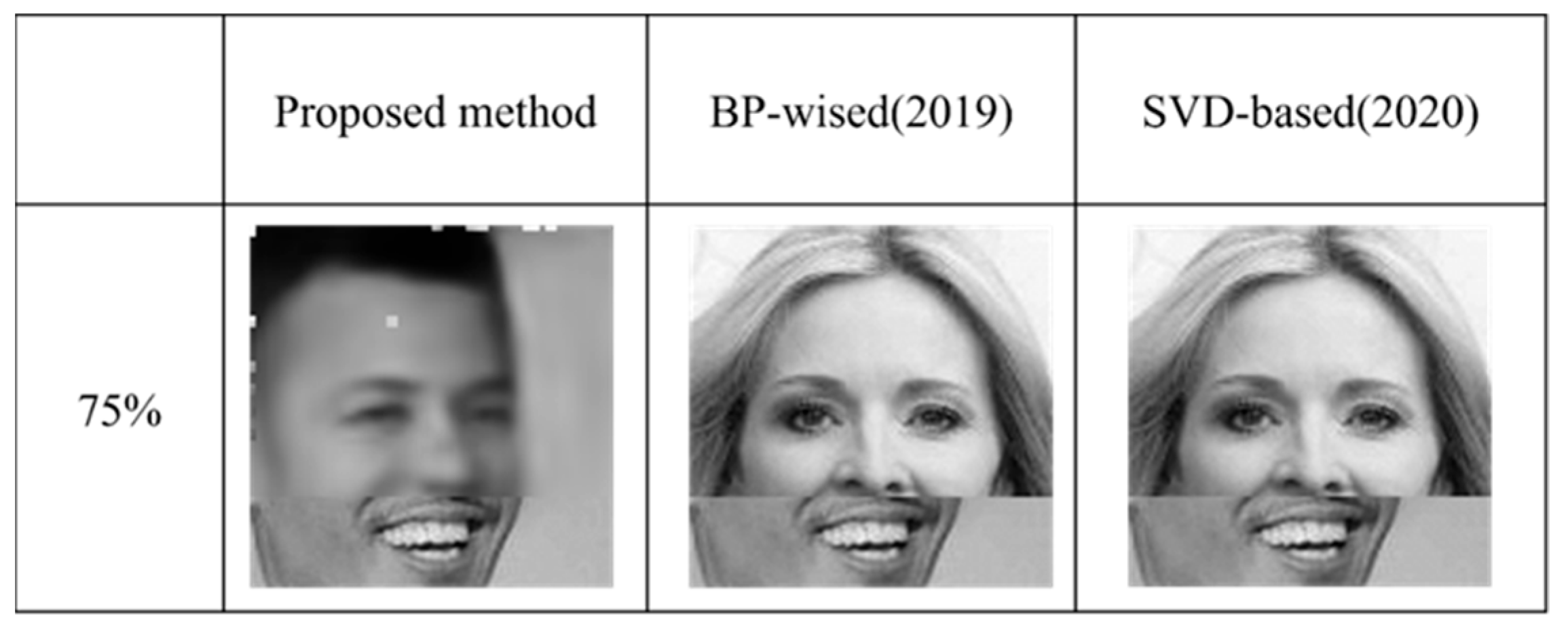
Figure 22 compares image recovery under 75% basic tampering using our method, BP-wised, and SVD-based. It clearly shows our method’s superior structural recovery under heavy tampering.
Table 13 compares localization performance under basic tampering. Data for other methods are referenced from Rezaei et al. [20]. Our method achieves high recall and F1-score, approaching 1, mainly due to fine-grained 2 × 2 block detection combined with morphological closing, which enhances localization accuracy.
The numerical performance metrics under collage attack are summarized in Table 10 (PSNR) and Table 11 (SSIM). The results confirm that the proposed method maintains high-quality reconstruction even under 75% tampering, with PSNR values above 32 dB and SSIM above 0.91. Experiments show that under heavy tampering, our method outperforms others. BP-wised and SVD-based methods, unable to effectively resist collage attacks, yield significantly lower performance, similar to results under basic tampering.
The proposed method outperforms previous approaches under high tampering rates. However, at lower tampering levels, detection accuracy is affected due to the limited effectiveness of morphological closing. As shown in Figure 23, under 75% collage attacks, our method demonstrates stronger resistance compared to BP-wised and SVD-based methods.
Table 14 shows the evaluation results for collage attack localization, with external data referenced from Rezaei et al. [20]. Overall, our method outperforms most existing approaches in F1-score, second only to Rezaei et al. [20].
In summary, the proposed method consistently outperforms baseline methods, especially under high tampering levels. It achieves superior SSIM and PSNR scores (e.g., SSIM = 0.943 at 75% tampering) and offers robust localization (F1-score = 0.999), demonstrating its practical utility and resilience where conventional methods degrade significantly. These results validate the advantages of a unified CAE-based design over traditional and dual network approaches.

5. Conclusions and Future Work

5.1. Conclusions

This study proposes a novel fragile watermarking method based on a convolutional autoencoder, which differs from traditional approaches that embed authentication and recovery data separately. By leveraging compact bottleneck features, encoded compression, and a block-wise voting mechanism, the proposed method maintains high structural similarity (SSIM) even under extensive tampering scenarios.
To enhance robustness against collage attacks, we integrated secret key-based pseudo-random scrambling with the Arnold Transform, effectively resisting over 50% patch-level replacements. Tamper localization is refined from 16 × 16 to 2 × 2 sub-blocks and further improved using morphological closing, thereby increasing localization granularity and pixel-level accuracy.
Overall, the proposed approach demonstrates robustness under high tampering ratios, effective resistance to collage attacks, and stable performance in both tamper localization and image self-recovery. For instance, at 75% tampering, the method still achieves an average SSIM of 0.943 and PSNR above 30 dB, underscoring its strong restoration ability in highly compromised images.

5.2. Future Work

Due to limited computational resources and dataset availability, this study currently focuses on facial image datasets and cannot be generalized to arbitrary images. In particular, we relied on the CelebA dataset, which, although popular for image restoration and watermarking tasks, is limited to facial images. The primary reason for employing CelebA in our experiments is its suitability for controlled training within a manageable time frame. Training on heterogeneous and large-scale generalized datasets would considerably extend and complicate the training process, making it difficult to ensure consistent convergence within a reasonable duration. In the future, we plan to extend our evaluation to standard benchmark images (e.g., Lena, Baboon, Peppers, Airplane) and other publicly available datasets that contain a wider variety of content types. This will allow for a more comprehensive validation of the method’s robustness and generalizability beyond facial data. In the future, this limitation could be addressed with increased computational power and access to diverse open-source image datasets, enabling the training of a more generalized restoration model.
In terms of security, while using a unique secret key per image enhances protection, it also introduces usability challenges. Future work will explore strategies to balance security with key management efficiency.
Additionally, adversarial attacks such as FGSM [34] have shown that small perturbations can mislead deep learning models. Since watermark embedding and image recovery also introduce perturbations, these may impact AI-based classifiers. As a countermeasure, we propose utilizing Principal Component Analysis (PCA) on bottleneck features extracted by the convolutional autoencoder. This allows classification tasks to rely directly on compact and meaningful embedded features, potentially improving model robustness even under tampering or restoration.
Finally, future work will incorporate deeper statistical analysis by reporting standard deviations, confidence intervals, and error margins for all evaluation metrics. This will provide a more rigorous understanding of the model’s consistency and performance variability across diverse testing scenarios.

Author Contributions

Conceptualization, C.-F.L. and I.-C.L.; methodology, T.-M.L. and A.U.R.; software, A.U.R.; validation, T.-M.L. and C.-F.L.; formal analysis, A.U.R. and I.-C.L.; investigation, A.U.R.; resources, I.-C.L.; data curation, A.U.R.; writing—original draft preparation, A.U.R.; writing—review and editing, I.-C.L. and C.-F.L.; visualization, A.U.R.; supervision, I.-C.L.; project administration, I.-C.L.; funding acquisition, I.-C.L. All authors have read and agreed to the published version of the manuscript.

Funding

This research was partially supported by the National Science and Technology Council of Taiwan (NSTC 113-2221-E-324-017-MY2).

Data Availability Statement

This study used the publicly available dataset: jessicali9530. (n.d.). CelebA dataset. Kaggle. Retrieved 8 April 2025, from https://www.kaggle.com/datasets/jessicali9530/celeba-dataset. All other data generated or analyzed during this study are included in this article, and further inquiries can be directed to the corresponding author.

Conflicts of Interest

The authors declare no conflicts of interest.

References

  1. Capasso, P.; Cattaneo, G.; De Marsico, M. A Comprehensive Survey on Methods for Image Integrity. ACM Trans. Multimed. Comput. Commun. Appl. 2024, 20, 34. [Google Scholar] [CrossRef]
  2. Lee, W.-B.; Chen, T.-H. A Public Verifiable Copy Protection Technique for Still Images. J. Syst. Softw. 2002, 62, 195–204. [Google Scholar] [CrossRef]
  3. Li, X.; Guo, M.; Wang, Z.; Li, J.; Qin, C. Robust Image Hashing in Encrypted Domain. IEEE Trans. Emerg. Top. Comput. Intell. 2024, 8, 670–683. [Google Scholar] [CrossRef]
  4. Honsinger, C.W. Book Review: Digital Watermarking. J. Electron. Imaging 2002, 11, 414. [Google Scholar] [CrossRef]
  5. Ferrara, P.; Bianchi, T.; De Rosa, A.; Piva, A. Image Forgery Localization via Fine-Grained Analysis of CFA Artifacts. IEEE Trans. Inf. Forensics Secur. 2012, 7, 1566–1577. [Google Scholar] [CrossRef]
  6. Jegou, H.; Douze, M.; Schmid, C. Hamming Embedding and Weak Geometric Consistency for Large Scale Image Search. In Computer Vision–ECCV 2008, Proceedings of the 10th European Conference on Computer Vision, Marseille, France, 12–18 October 2008; Forsyth, D., Torr, P., Zisserman, A., Eds.; Springer: Berlin/Heidelberg, Germany, 2008; Volume 5302, pp. 304–317. [Google Scholar]
  7. Li, L.; Li, S.; Zhu, H.; Chu, S.-C.; Roddick, J.F.; Pan, J.-S. An Efficient Scheme for Detecting Copy-move Forged Images by Local Binary Patterns. J. Inf. Hiding Multim. Signal Process. 2013, 4, 46–56. [Google Scholar]
  8. Mushtaq, S.; Mir, A.H. Digital Image Forgeries and Passive Image Authentication Techniques: A Survey. Int. J. Adv. Sci. Technol. 2014, 73, 15–32. [Google Scholar] [CrossRef]
  9. Yang, C.-W.; Shen, J.-J. Recover the Tampered Image Based on VQ Indexing. Signal Process. 2010, 90, 331–343. [Google Scholar] [CrossRef]
  10. Di, Y.; Lee, C.; Wang, Z.; Chang, C.; Li, J. A Robust and Removable Watermarking Scheme Using Singular Value Decomposition. KSII Trans. Internet Inf. Syst. 2016, 10, 5268–5285. [Google Scholar] [CrossRef]
  11. Singh, D.; Singh, S. Effective self-embedding watermarking scheme for image tampered detection and localization with recovery capability. J. Vis. Commun. Image Represent. 2016, 38, 775–789. [Google Scholar] [CrossRef]
  12. Qin, C.; Ji, P.; Zhang, X.; Dong, J.; Wang, J. Fragile image watermarking with pixel-wise recovery based on overlapping embedding strategy. Signal Process. 2017, 138, 280–293. [Google Scholar] [CrossRef]
  13. Lee, C.; Shen, J.; Chen, Z.; Agrawal, S. Self-Embedding Authentication Watermarking with Effective Tampered Location Detection and High-Quality Image Recovery. Sensors 2019, 19, 2267. [Google Scholar] [CrossRef]
  14. Lee, C.-F.; Shen, J.-J.; Hsu, F.-W. A Survey of Semi-Fragile Watermarking Authentication. In Recent Advances in Intelligent Information Hiding and Multimedia Signal Processing; Pan, J.-S., Ito, A., Tsai, P.-W., Jain, L., Eds.; Smart Innovation, Systems and Technologies; Springer: Cham, Switzerland, 2019; Volume 109. [Google Scholar] [CrossRef]
  15. Rakhmawati, L.; Wirawan, W.; Suwadi, S. A recent survey of self-embedding fragile watermarking scheme for image authentication with recovery capability. EURASIP J. Image Video Process. 2019, 22, 61. [Google Scholar] [CrossRef]
  16. Lecun, Y.; Bottou, L.; Bengio, Y.; Haffner, P. Gradient-based learning applied to document recognition. Proc. IEEE 1998, 86, 2278–2324. [Google Scholar] [CrossRef]
  17. Theis, L.; Shi, W.; Cunningham, A.; Huszár, F. Lossy Image Compression with Compressive Autoencoders. arXiv 2017, arXiv:1703.00395. [Google Scholar] [CrossRef]
  18. Li, P.; Pei, Y.; Li, J. A comprehensive survey on design and application of autoencoder in deep learning. Appl. Soft. Comput. 2023, 138, 21. [Google Scholar] [CrossRef]
  19. Shen, J.-J.; Lee, C.-F.; Hsu, F.-W.; Agrawal, S. A Self-Embedding Fragile Image Authentication Based on Singular Value Decomposition. Multimed. Tools Appl. 2020, 79, 25969–25988. [Google Scholar] [CrossRef]
  20. Rezaei, M.; Taheri, H. Digital image self-recovery using CNN networks. Optik 2022, 264, 12. [Google Scholar] [CrossRef]
  21. Zhang, X.; Wang, S. Fragile Watermarking with Error-Free Restoration Capability. IEEE Trans. Multimed. 2008, 10, 1490–1499. [Google Scholar] [CrossRef]
  22. Li, C.; Wang, Y.; Ma, B.; Zhang, Z. A novel self-recovery fragile watermarking scheme based on dual-redundant-ring structure. Comput. Electr. Eng. 2011, 37, 927–940. [Google Scholar] [CrossRef]
  23. Chow, Y.-W.; Susilo, W.; Tonien, J.; Zong, W. A QR Code Watermarking Approach Based on the DWT-DCT Technique. In Information Security and Privacy–ACISP 2017, Proceedings of the 22nd Australasian Conference on Information Security and Privacy, Auckland, New Zealand, 3–5 July 2017; Lai, J., Ed.; Springer: Cham, Switzerland, 2017; Volume 10343, pp. 314–331. [Google Scholar]
  24. Jiang, F.; Tao, W.; Liu, S.; Ren, J.; Guo, X.; Zhao, D. An End-to-End Compression Framework Based on Convolutional Neural Networks. IEEE Trans. Circuits Syst. Video Technol. 2018, 28, 3007–3018. [Google Scholar] [CrossRef]
  25. Padhi, S.K.; Tiwari, A.; Ali, S.S. Deep Learning-Based Dual Watermarking for Image Copyright Protection and Authentication. IEEE Trans. Artif. Intell. 2024, 5, 6134–6145. [Google Scholar] [CrossRef]
  26. Ben Jabra, S.; Ben Farah, M. Deep Learning-Based Watermarking Techniques Challenges: A Review of Current and Future Trends. Circ. Syst. Signal Process. 2024, 43, 4339–4368. [Google Scholar] [CrossRef]
  27. Bui, T.; Agarwal, S.; Yu, N.; Collomosse, J. Rosteals: Robust Steganography Using Autoencoder Latent Space. In Proceedings of the IEEE/CVF Conference on Computer Vision and Pattern Recognition (CVPR), Vancouver, BC, Canada, 18–22 June 2023; pp. 933–942. [Google Scholar]
  28. Simonyan, K.; Zisserman, A. Very Deep Convolutional Networks for Large-Scale Image Recognition. arXiv 2014, arXiv:1409.1556. [Google Scholar]
  29. Wang, Z.; Bovik, A.; Sheikh, H.; Simoncelli, E. Image quality assessment: From error visibility to structural similarity. IEEE Trans. Image Process. 2004, 13, 600–612. [Google Scholar] [CrossRef] [PubMed]
  30. jessicali9530. (n.d.). CelebA dataset. Kaggle. Available online: https://www.kaggle.com/datasets/jessicali9530/celeba-dataset (accessed on 8 April 2025).
  31. OpenCV Team. Color Conversions. Available online: https://docs.opencv.org/4.x/de/d25/imgproc_color_conversions.html (accessed on 17 May 2025).
  32. Sarreshtedari, S.; Akhaee, M. A Source-Channel Coding Approach to Digital Image Protection and Self-Recovery. IEEE Trans. Image Process. 2015, 24, 2266–2277. [Google Scholar] [CrossRef] [PubMed]
  33. Yuan, X.; Li, X.; Liu, T. Gauss-Jordan elimination-based image tampering detection and self-recovery. Signal Process.-Image Commun. 2021, 90, 14. [Google Scholar] [CrossRef]
  34. Goodfellow, I.J.; Shlens, J.; Szegedy, C. Explaining and Harnessing Adversarial Examples. arXiv 2014, arXiv:1412.6572. [Google Scholar]
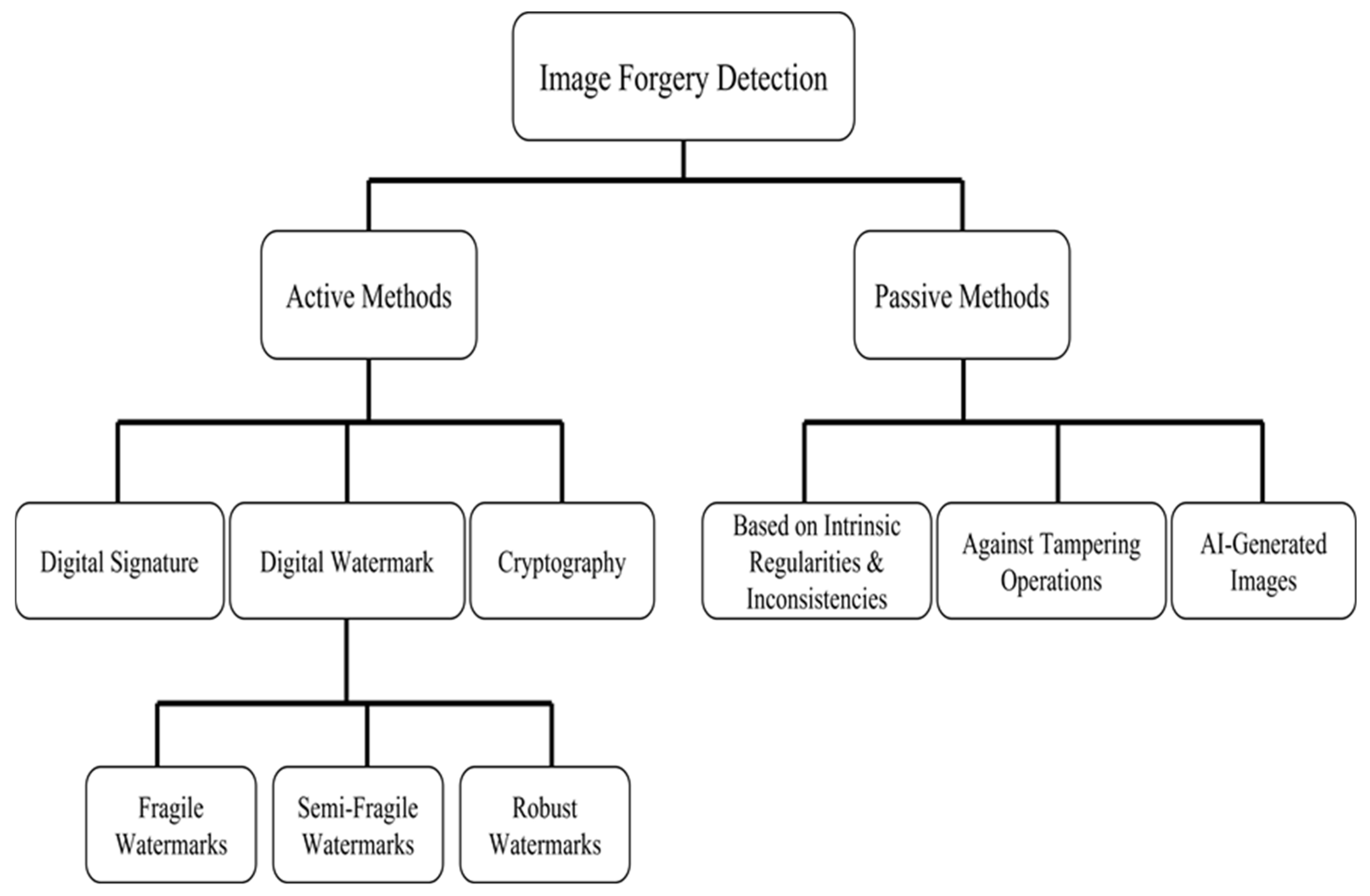
Figure 1. Image authentication methods.
Electronics 14 03595 g001
Figure 2. Fragile watermarking framework.
Electronics 14 03595 g002
Figure 3. Recovery data generation using CNN-based ComCNN and RecCNN [20].
Electronics 14 03595 g003
Figure 4. Watermark generation and embedding flowchart.
Electronics 14 03595 g004
Figure 5. Simplified model architecture of the encoder and decoder, based on VGG11 structure.
Electronics 14 03595 g005
Figure 6. Illustration of generating multiple copies of the bottleneck vector for embedding.
Electronics 14 03595 g006
Figure 7. Scrambling of bottleneck features using number sequence and Arnold Transform.
Electronics 14 03595 g007
Figure 8. Flowchart of tampering localization and self-recovery.
Electronics 14 03595 g008
Figure 9. Descrambling bottleneck blocks using inverse Arnold Transform.
Electronics 14 03595 g009
Figure 10. Tampering detection voting process.
Electronics 14 03595 g010
Figure 11. Sample experimental images.
Electronics 14 03595 g011
Figure 12. Network design comparisons. (a) Architecture without fully connected layers. (b) Architecture with fully connected layers.
Electronics 14 03595 g012
Figure 13. (a) Results without using fully connected network; (b) Results of using fully connected layers.
Electronics 14 03595 g013
Figure 14. Comparison of different numbers of bottlenecks. The labels indicate different configurations: (a) FC-16, (b) FC-32, (c) FC-64, (d) FC-128, and (e) FC-256.
Electronics 14 03595 g014
Figure 15. Tampering attack simulation (adding glasses).
Electronics 14 03595 g015
Figure 16. Tampering attack simulation (graffiti text).
Electronics 14 03595 g016
Figure 17. Collage attack simulation.
Electronics 14 03595 g017
Figure 18. Tampering detection and recovery results under basic tampering at 10%, 50%, and 75% levels. (ac) tampered images; (df) detected tampered regions; (gi) recovered images.
Electronics 14 03595 g018
Figure 19. Tampering detection and recovery results under collage attacks at 10%, 40%, and 75% tampering levels. (ac) Tampered collage images. (df) Detected tampered regions (binary masks). (gi) Recovered outputs.
Electronics 14 03595 g019
Figure 20. Comparison of tampered block recovery quality at different tampering rates (PSNR (dB)) using several methods: Sarrshteadari et al. Method (2LSB) [32], BP-wised Method (Padhi et al., 2019 [13]), SVD-based Method (Ganic & Eskicioglu, 2020 [19]), Yuan et al. Method (Yuan et al., 2021 [33]), Rezaei et al. Method (Rezaei & Taheri, 2022 [20]), and the Proposed Method.
Electronics 14 03595 g020
Figure 21. Comparison of tampered block recovery quality at different tampering rates (SSIM). using BP-wised Method (2019) [13]; SVD-based Method (2020) [19]; Rezaei et al. Method (2022 [20]).
Electronics 14 03595 g021
Figure 22. Comparison of 75% basic tampering attack with BP-wised and SVD-based methods.
Electronics 14 03595 g022
Figure 23. Recovery results under 75% collage attacks.
Electronics 14 03595 g023
Table 1. Symbol definitions.
No.NotationDescription
(1) I O original image
(2)Wweight of the original image
(3)Hheight of the original image
(4) B i , i = ( 1 ,   2 , ,   N ) every block in the original image
(5) m × n size of a block
(6) N total number of blocks in an image
(7)SKsecret key (Generate block-mapping sequence)
(8)Vbottleneck
(9) | | V | | bottleneck length is represented in bytes
(10) V 2 d reshape the bottleneck into a 2D format
(11) v take the square root of the length of the bottleneck (to convert it into the side length of a 2D shape) i.e., | | V | | = v 2
(12) B M i , i = ( 1 ,   2 , ,   N ) mapping block
(13) R i recovery code of each block
(14) M r m i , i = ( 1 ,   2 , ,   N ) mapping block recovery data
(15) A i , i = ( 1 ,   2 , ,   N ) authentication code of each block
(16) I W watermarked image
(17) I T tampered image
(18)   A i , i = ( 1 ,   2 , ,   N ) authentication message (receiver)
(19) I R recovered image
(20)thyperparameter for designing the number of neurons
(21)Tnumber of Arnold Transform iterations
Table 2. Performance comparison across different depths (average on 10,000 test images).
Model ArchitecturePSNRSSIM
(a)28.4170.803
(b)28.5810.849
(c)28.5830.850
(d)28.3280.796
Table 3. Comparison of models with and without batch normalization (averaged on 10,000 test images).
Model ArchitecturePSNRSSIM
(a)28.5830.850
(b)29.1600.906
Table 4. Results for different numbers of bottlenecks (average over 10,000 test images).
Model ArchitecturePSNRSSIM
(a) FC-1628.6640.857
(b) FC-3228.8460.879
(c) FC-6429.2970.921
(d) FC-12829.2990.927
(e) FC-25629.3510.939
Table 5. Image quality after watermark embedding (average over 10,000 test images).
PSNRSSIM
(a)43.6540.999
Table 6. Recovered image quality for various tampering levels.
Tampering Level0%10%20%30%40%50%60%70%75%
PSNR (dB)43.65437.96435.74234.28233.16232.23831.38330.78730.518
SSIM0.9990.9910.9840.9770.9710.9630.9530.9460.943
Table 7. Recovery quality of tampered regions at different tampering levels.
Tampering Level0%10%20%30%40%50%60%70%75%
PSNR (dB)43.65429.46229.43229.46829.49229.39029.31129.32429.322
SSIM0.9990.8120.8720.9080.9220.9210.9200.9240.924
Table 8. Effect of different tampering levels on tampering detection and localization (average over 10,000 test images).
Tampering Level0%10%20%30%40%50%60%70%75%
Recall-0.9990.9990.9990.9990.9990.9990.9990.999
Precision-0.9410.9840.9890.98410.9890.9951
F1-Score-0.9690.9920.9940.9920.9990.9940.9970.999
Table 9. Recovered image quality under different collage attack levels.
Tampering Level0%10%20%30%40%50%60%70%75%
PSNR (dB)43.65437.96435.74234.28233.14032.21831.36430.77130.502
SSIM0.9990.9910.9840.9770.9580.9500.9380.9320.929
Table 10. Recovery quality of tampered regions under various collage attack levels.
Tampering Level0%10%20%30%40%50%60%70%75%
PSNR (dB)43.65429.39729.40229.42529.46629.36829.2929.30729.306
SSIM0.9990.6640.790.8440.8870.8940.8960.9040.906
Table 11. Tampering localization performance at different collage attack levels.
Tampering Level0%10%20%30%40%50%60%70%75%
Recall-0.9650.9820.9780.9850.9880.9870.9890.99
Precision-0.9650.9840.990.98410.990.9951
F1-Score-0.9650.9830.9840.9850.9940.9890.9920.995
Table 12. Image quality after watermark embedding.
MethodPSNRSSIM
BP-wised (2019) [13]44.1630.999
SVD-based (2020) [19]44.0130.999
Rezaei et al. (2022) [20]44.2-
Proposed Method43.6540.999
Table 13. Detection and localization quality of basic tampering attacks.
SchemesTamper Rate10%20%40%
Sarreshtedari et al. [32]
(2015)
Recall111
Precision111
F1-Score111
BP-wised [13]
(2019)
Recall0.9990.9991
Precision0.8390.9140.984
F1-Score0.9120.9550.992
SVD-based [19]
(2020)
Recall0.9990.9990.999
Precision0.9390.9430.984
F1-Score0.9680.9710.992
Yuan et al. [33]
(2021)
Recall0.9880.9640.899
Precision0.9560.9350.817
F1-Score0.9710.9490.856
Rezaei et al. [20]
(2022)
Recall0.9950.9910.978
Precision111
F1-Score0.9970.9950.988
ProposedRecall0.9990.9990.999
Precision0.9410.9840.984
F1-Score0.9690.9920.992
Table 14. Collage attack tampering detection and localization results.
SchemesTamper Rate10%20%40%
Sarreshtedari et al. [32]
(2015)
Recall0.4030.2370.112
Precision111
F1-Score0.5740.3830.201
BP-wised [13]
(2019)
Recall0.0620.0620.047
Precision0.2450.3980.752
F1-Score0.0990.1070.089
SVD-based [19]
(2020)
Recall0.0620.0150.015
Precision0.4900.2310.504
F1-Score0.1100.0290.030
Yuan et al. [33]
(2021)
Recall0.9820.9690.897
Precision0.9560.9310.812
F1-Score0.9680.9490.852
Rezaei et al. [20]
(2022)
Recall0.9960.9910.977
Precision111
F1-Score0.9970.9950.988
ProposedRecall0.9650.9820.985
Precision0.9650.9840.984
F1-Score0.9650.9830.985
Disclaimer/Publisher’s Note: The statements, opinions and data contained in all publications are solely those of the individual author(s) and contributor(s) and not of MDPI and/or the editor(s). MDPI and/or the editor(s) disclaim responsibility for any injury to people or property resulting from any ideas, methods, instructions or products referred to in the content.