Abstract
Lithium-ion batteries (LIBs) are critical components in safety-critical systems such as electric vehicles, aerospace, and grid-scale energy storage. Their degradation over time can lead to catastrophic failures, including thermal runaway and uncontrolled combustion, posing severe threats to human safety and infrastructure. Developing a robust AI framework for degradation prognostics in safety-critical systems is essential to mitigate these risks and ensure operational safety. However, sensor noise, dynamic operating conditions, and the multi-scale nature of degradation processes complicate this task. Traditional denoising and modeling approaches often fail to preserve informative temporal features or capture both abrupt fluctuations and long-term trends simultaneously. To address these limitations, this paper proposes a hybrid data-driven framework that combines Sample Entropy-guided Variational Mode Decomposition (SE-VMD) with K-means clustering for adaptive signal preprocessing. The SE-VMD algorithm automatically determines the optimal number of decomposition modes, while K-means separates high- and low-frequency components, enabling robust feature extraction. A dual-branch architecture is designed, where Gated Recurrent Units (GRUs) extract short-term dynamics from high-frequency signals, and Transformers model long-term trends from low-frequency signals. This dual-branch approach ensures comprehensive multi-scale degradation feature learning. Additionally, experiments with varying sliding window sizes are conducted to optimize temporal modeling and enhance the framework’s robustness and generalization. Benchmark dataset evaluations demonstrate that the proposed method outperforms traditional approaches in prediction accuracy and stability under diverse conditions. The framework directly contributes to Artificial Intelligence for Security by providing a reliable solution for battery health monitoring in safety-critical applications, enabling early risk mitigation and ensuring operational safety in real-world scenarios.
1. Introduction
Lithium-ion batteries (LIBs), critical components in safety-critical systems such as electric vehicles (EVs), portable electronics, and grid-scale energy storage [1,2,3], are widely adopted due to their high energy density and long cycle life. However, repeated charge–discharge cycles inevitably cause performance degradation, primarily characterized by capacity fade and elevated internal resistance. These degradation mechanisms not only reduce the battery’s power delivery capability but also introduce severe safety hazards, including thermal runaway and catastrophic failures. Real-world incidents underscore the economic and operational risks of unmonitored battery aging. For instance, in 2007, Sony recalled 9.6 million laptops due to abnormal battery aging, resulting in direct economic losses of up to $430 million [4]. Similarly, in 2018, a fire broke out in a lithium-ion battery pack at a cement plant in South Korea due to aging, resulting in losses exceeding $3 million [5]. These cases emphasize the critical need for secure and robust degradation prediction systems that can accurately track degradation patterns. Such systems enable proactive maintenance strategies, mitigating risks in safety-critical applications like EVs and industrial energy storage. Developing reliable frameworks for degradation prognostics is therefore essential to ensure operational safety, prevent costly failures, and extend the service life of LIBs in high-stakes environments.
Nevertheless, building a degradation prognostics model that achieves both high accuracy and strong robustness remains a significant challenge. First, sensor noise and variable operating conditions reduce the signal-to-noise ratio of the acquired capacity data, making it difficult for traditional denoising methods to effectively remove noise while retaining useful information. Second, battery capacity degradation exhibits multi-scale characteristics, involving high-frequency random fluctuations and low-frequency gradual trends, which are challenging for single time-series models to capture simultaneously. Additionally, the key parameters of existing models—such as sliding window lengths—are often determined empirically, lacking clear connections to the heterogeneous degradation dynamics across different datasets. This limitation restricts their generalization ability in diverse application scenarios.
To address these challenges and advance Artificial Intelligence for Security, this study proposes a robust AI framework combining Sample Entropy-Guided Variational Mode Decomposition (SE-VMD) and a dual-branch hybrid neural network. The framework enhances both battery safety through accurate degradation prediction and AI robustness through adaptive temporal modeling.
The following key contributions of this paper are as follows:
- (1)
- A Frequency-Aware Dual-Branch Architecture for Multi-Scale Degradation Modeling: We propose a novel dual-branch deep learning framework that explicitly models both abrupt and gradual degradation patterns in LIBs. High-frequency dynamics (e.g., sudden capacity drops) are captured by Gated Recurrent Units (GRUs), while low-frequency trends (e.g., long-term capacity fade) are modeled by Transformers. A learnable fusion module dynamically integrates these pathways based on their temporal characteristics, enhancing robustness against noise, adversarial perturbations, and heterogeneous aging behaviors. This architecture enables reliable generalization—particularly critical in safety-critical applications where false negatives may lead to catastrophic failures.
- (2)
- Adaptive and Interpretable Signal Decomposition for Frequency-Specific Feature Extraction: To enable the frequency-aware design of the dual-branch model, we introduce an adaptive decomposition strategy combining Sample Entropy-based Variational Mode Decomposition (SE-VMD) with K-means clustering. SE-VMD automatically determines the optimal number of intrinsic mode functions (IMFs) by minimizing sample entropy, eliminating the need for manual parameter tuning. Subsequently, IMFs are grouped into high- and low-frequency components using a hybrid feature space (frequency centroid and sample entropy), ensuring both physical interpretability and robustness to measurement noise. This decomposition provides a principled, data-driven basis for routing signals to specialized subnetworks.
- (3)
- Systematic Empirical Guidelines for Temporal Context Selection in Battery Prognostics: We conduct a comprehensive experimental study on the impact of sliding window size—a critical yet often overlooked hyperparameter—in battery degradation modeling. Our results demonstrate that window length significantly affects both decomposition quality and model performance, with an optimal range yielding the best trade-off between short-term responsiveness and long-term trend stability. These findings provide actionable design principles for configuring temporal context in real-world battery health monitoring systems, improving prediction reliability across diverse aging scenarios.
2. Literature Review
The imperative to monitor capacity degradation in LIBs has driven interdisciplinary research, leading to two critical quantitative metrics: State of Health (SOH) and Remaining Useful Life (RUL). SOH is defined as the ratio of a battery’s current maximum capacity to its rated capacity [6], while RUL quantifies the remaining charge–discharge cycles until the battery reaches its minimum acceptable capacity threshold (typically 70–80% of initial capacity) [7]. Accurate and timely RUL prediction is vital for early risk detection and proactive safety management, particularly in security-critical applications such as electric vehicles and grid-scale energy storage systems. As degradation progresses with repeated cycling, precise SOH/RUL estimation enables real-time maintenance scheduling and resource optimization to mitigate sudden failures. Current methodologies for LIB degradation prognostics fall into three categories:
2.1. Physics-Based Models
Physics-based models simulate battery behavior using electrochemical equations, equivalent circuits, or empirical statistics [8]. For example, Li et al. [9] developed a multi-layer thermal model, while Chen et al. [10] proposed a fractional-order impedance model to describe internal degradation mechanisms such as lithium dendrite growth. Although these models provide physical insights, they often require complex parameter calibration and high computational costs, limiting their adaptability under dynamic operating conditions.
Equivalent circuit models (ECMs), such as the DWRLS method [11] and piecewise nonlinear models [12], improve real-time performance by simplifying internal dynamics but tend to overlook hidden state changes and temperature-current coupling effects, resulting in prediction inaccuracies during abrupt capacity drops. Statistical regression models [13] avoid reliance on physical knowledge but struggle with complex noise and nonlinear degradation patterns.
2.2. Data-Driven Approaches
Data-driven methods extract degradation patterns directly from historical data without requiring detailed physical knowledge. These approaches treat the battery as a “black box” and use machine learning techniques to map aging features to health indicators [14].
Statistical models like ARIMA [15] are simple and interpretable but lack the capability to model long-term nonlinear dependencies. Gaussian Processes (GP) [16] offer uncertainty quantification but suffer from accuracy degradation under varying environmental conditions—a limitation also observed in traditional simulation-based RUL frameworks that lack sufficient historical data. Machine learning techniques such as SVM [17] and deep learning models including CNNs, RNNs, LSTMs, and GRUs [18,19,20,21,22,23] have shown strong feature extraction capabilities, though they often incur high computational costs when modeling long sequences. Recently, Transformer-based architectures [24,25] have gained popularity due to their ability to capture long-range dependencies via self-attention mechanisms.
To enhance robustness under practical constraints, recent works address key challenges such as few-shot learning, uncertainty interference, and temporal data masking. For instance, BayesMRG [26] introduces a Bayesian meta-learning framework with random graph representation to handle sparse labeled data and uncertainty in LIB RUL prediction, achieving over 40% error reduction on public datasets. In another direction, a progressive learning approach [27] tackles temporal data masking—common in cloud-based BMS—by generating masked samples during training and enabling robust inference even at 70% masking ratios. Meanwhile, temporal deep learning frameworks incorporating uncertainty representation through quantile regression and kernel density estimation [28] enable probabilistic SOH estimation, improving reliability in safety-critical scenarios. However, relying solely on a single model may limit the ability to fully characterize diverse temporal dynamics, affecting generalization performance.
2.3. Hybrid Strategies
According to the No-Free-Lunch (NFL) theorem, no single model is optimal for all tasks. Hybrid strategies combine complementary methods to overcome individual limitations and enhance prediction accuracy. For instance, Auto-CNN-LSTM [29] integrates deep CNN and LSTM to extract hierarchical spatiotemporal features from degradation data. Reference [18] proposes a CNN-LSTM architecture for State of Charge (SOC) estimation, leveraging CNN’s spatial feature extraction and LSTM’s temporal modeling. Similarly, SFTTN [30] employs 2D-CNN and BiLSTM layers to learn domain-invariant features for cross-temperature SOC prediction. In [31], a two-stage optimized graph convolutional network (GCN) was connected to an LSTM with dual attention mechanisms to jointly predict SOH and RUL, allowing the model to focus on critical time steps and improving interpretability. This trend toward attention-enhanced hybrid models is further supported by recent work in fault diagnosis [32], demonstrating the broad effectiveness of adaptive feature weighting in time-series analysis under noisy conditions.
To address noise in degradation signals, several studies incorporate advanced signal preprocessing methods. A CEEMDAN-based smoothing framework [33] decomposes noisy signals before feeding them into an LSTM for RUL prediction. This method achieves high accuracy and robustness on NASA and CALCE datasets. However, CEEMDAN is computationally intensive and sensitive to parameter settings, with residual high-frequency noise potentially affecting component stability. Similarly, EEMD has been used in an EEMD-GRU-MLR hybrid model [34], where high-frequency components are modeled by GRU and low-frequency trends by MLR. While this approach reduces prediction errors compared to standalone models, EEMD suffers from mode mixing and limited computational efficiency. Moreover, MLR cannot adequately capture nonlinear degradation patterns, and residual noise from decomposition increases GRU output volatility.
Compared to EMD-family methods, VMD offers a more structured approach to frequency-constrained decomposition by optimizing both center frequencies and bandwidths of each mode. This enables better separation of high- and low-frequency components in non-stationary signals, provided that the number of modes (K) and penalty factor (α) are appropriately selected. Additionally, VMD’s explicit frequency constraints improve noise suppression by localizing noise energy in specific modes, which can be filtered out during post-processing.
The rest of the paper is structured as follows: Section 3 introduces the proposed method, combining SE-VMD for signal preprocessing with a dual-branch GRU-Transformer network for multi-scale degradation modeling. Section 4 describes the experimental setup, datasets, and performance comparisons under different sliding window sizes. Section 5 concludes the paper.
3. Methodology
3.1. Overview
As illustrated in Figure 1, the proposed methodology consists of the following key steps:
3.1.1. Battery Degradation Indicator Selection
Battery capacity is selected as the primary health indicator to quantify the progressive performance loss of LIBs. The capacity is computed from raw sensor data, including cell current (I), cell voltage (V), and time (t), collected during charge–discharge cycles. Specifically, the discharge capacity is obtained by integrating the current over time within a full discharge cycle, where the start and end points are determined by voltage cutoff thresholds. The detailed procedure follows the standardized method described in [35], ensuring consistency with industry benchmarks. Temperature (T) is not used in the capacity estimation or subsequent modeling in this study.
3.1.2. Sequence Segmentation via Sliding Window Technique
To convert the raw time series data into a supervised learning format, a sliding window-based segmentation strategy is applied. A fixed-length time window with a defined step size is used to slice the sequence into input-output pairs. Specifically, given a time series , the first W points are taken as input features, and the (W + 1)-th point serves as the output label. The window then slides forward by the specified step size to form the next sample. This process continues until the end of the sequence.
The window size significantly impacts prediction performance: too short a window may lose long-term trends, while too large a window introduces redundancy. Therefore, we conduct comparative experiments in Section 4.3 to investigate the influence of different window sizes on model accuracy.
3.1.3. Signal Decomposition Using Sample Entropy-Guided VMD (SE-VMD)
The capacity sequence is adaptively decomposed into intrinsic mode functions (IMFs) using SE-VMD, which leverages sample entropy to automatically determine the optimal IMF count, reducing manual intervention and mode mixing. Subsequent K-means clustering separates IMFs into high-frequency (HF) and low-frequency (LF) subgroups, isolating abrupt changes from gradual degradation trends. This preprocessing step enhances feature interpretability and modeling robustness (see Section 3.2.2 for implementation details). Notably, the clustering is configured with two groups to reflect the bimodal nature of battery degradation—long-term trends and short-term fluctuations—while intermediate-frequency components are not explicitly modeled due to their limited dominance and consistency across diverse aging patterns.
3.1.4. Dual-Branch Temporal Modeling with Transformer and GRU Networks
Based on the HF and LF component sequences obtained in step (3), two sub-models are constructed: one based on the Transformer and the other on the Gated Recurrent Unit (see Section 3.3 for implementation details).
3.1.5. Degradation Prognostics and SOH Estimation
The trained model is applied to the test dataset to predict unknown capacity values. These predictions are then used to compute the State of Health (SOH), which quantitatively reflects the extent of battery degradation. This approach not only improves prediction accuracy but also provides meaningful insights into the battery’s aging behavior throughout its lifecycle.

Figure 1.
Flowchart of the Proposed Methodology.
3.2. Signal Decomposition
3.2.1. Traditional VMD Methodology
Based on window segmentation, the VMD algorithm is applied to decompose the raw battery capacity signal. Previous studies have employed Empirical Mode Decomposition (EMD) or its improved variant [36,37], Complete Ensemble EMD with Adaptive Noise (CEEMDAN), to extract noise components from LIB degradation data. While these methods offer greater adaptability compared to wavelet packet decomposition, they are susceptible to mode mixing and endpoint effects, which can distort the physical interpretation of the decomposition results. For example, in LIB capacity signals, EMD/CEEMDAN may confuse HF measurement noise with low-frequency degradation trends, leading to misinterpretation of the decomposition results. In contrast, VMD formulates signal decomposition as a constrained variational optimization problem, thereby enhancing robustness and interpretability. It iteratively optimizes a set of modes in the frequency domain, each with distinct center frequencies and bandwidths, ensuring spectral separation between components. This alignment with physical degradation mechanisms has been validated in [38,39], where VMD decomposition modes corresponded to distinct degradation stages. The detailed steps of the VMD decomposition process are outlined below:
Step 1: Construction of the Variational Model. The original capacity signal of the LIB is decomposed into k intrinsic mode functions (IMFs).
where denotes the Dirac delta function, * represents the convolution operation, is the partial derivative with respect to time t, and is the L2 norm.
This formulation minimizes the bandwidth of each IMF around its adaptively estimated central frequency . It provides a sparse, physically meaningful separation of the continuous signal into distinct dynamic components—such as long-term degradation, transient regeneration, and noise—each occupying a compact frequency band. This promotes modal clarity and avoids mode mixing seen in EMD-based methods. Compared to a continuous distribution, this approach ensures clearer physical interpretation and more accurate decomposition of the signal’s underlying dynamics.
Step 2: Introduction of Penalty Factors and Lagrange Multipliers
To transform the constrained variational problem into an unconstrained one, a quadratic penalty factor and a Lagrange multiplier are introduced. The augmented Lagrangian function is expressed as:
Step 3: ADMM-Based Optimization
Initialize{}, {}, {} and set the iteration counter n = 1. In the Fourier transform domain, the Alternating Direction Method of Multipliers (ADMM) is used to update{}, {}, {} for searching the saddle point of the above equation. The update formulas are as follows:
where denotes the noise tolerance parameter.
Step 4: Termination Criterion
The iteration continues until the stopping criterion is satisfied:
Taking battery B0005 as an example, the VMD algorithm was employed to decompose its capacity signal into seven distinct modes, denoted as Mode 1 through Mode 7. These modes are arranged in ascending order of frequency. As illustrated in Figure 2, an evident degradation trend in battery capacity is observed with increasing cycle numbers. Notably, during this decline, instances of capacity regeneration are also apparent. Modes 5–7 exhibit similar fluctuation patterns, which is consistent with their nature as high-frequency components that primarily capture measurement noise and minor signal variations rather than distinct degradation dynamics.
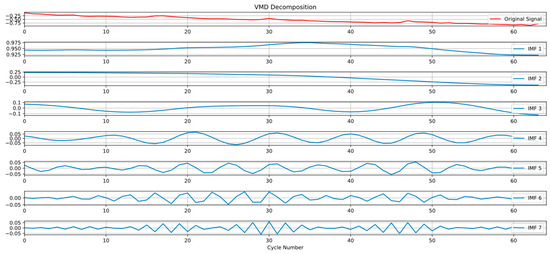
Figure 2.
B0005 capacity sequence decomposition based on VMD.
While VMD effectively addresses mode mixing and endpoint effects, its reliance on a fixed decomposition mode count k introduces limitations for battery degradation signals with dynamic complexity. An inappropriate k value can lead to under-decomposition (insufficient separation of meaningful components) or over-decomposition (excessive redundancy, particularly in high-frequency modes). In practice, k is often selected empirically—based on prior knowledge, reconstruction error, or mode interpretability. However, this empirical selection of k lacks adaptability: the optimal number of modes may vary across different batteries, aging stages, or operating conditions. A fixed k may fail to capture evolving signal complexity—such as transient regeneration events or changing noise levels—leading to suboptimal decomposition. This highlights a critical limitation of conventional VMD and underscores the need for adaptive or self-optimizing methods that can automatically determine k based on the intrinsic characteristics of the signal. Automatically identifying the optimal k would enhance model robustness, reduce human bias, and enable more accurate, generalizable feature extraction across diverse battery datasets.
3.2.2. Sample Entropy-Guided VMD with K-Means Clustering for Adaptive Signal Separation
To address the limitations of traditional VMD, we propose an improved algorithm that integrates sample entropy for adaptive mode selection and K-means clustering for frequency separation. This enhanced framework ensures decomposition complexity aligns with signal characteristics while achieving precise temporal-frequency domain partitioning. The complete implementation procedure is described in Algorithm 1, with the corresponding workflow illustrated in Figure 3.
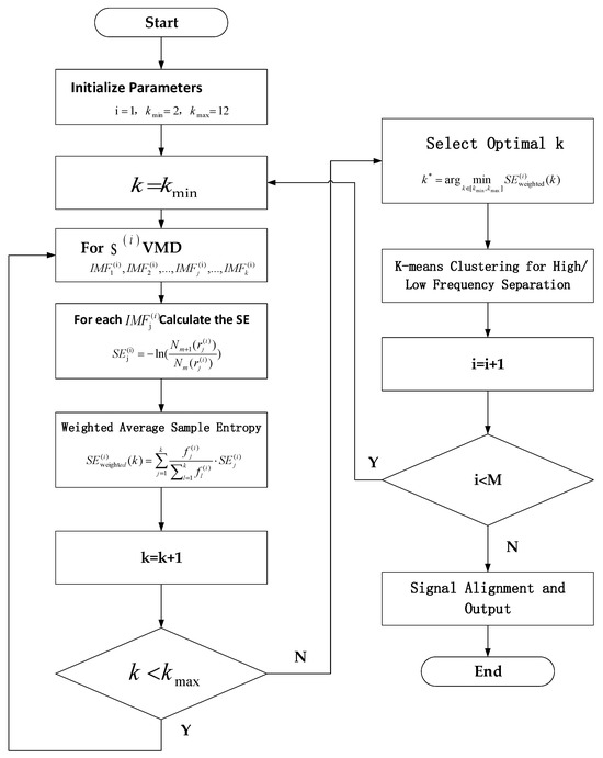
Figure 3.
Workflow Diagram of the Improved VMD Algorithm Incorporating Sample Entropy and K-Means Clustering.
| Algorithm 1: Sample Entropy-Guided VMD with K-means Clustering for Adaptive Signal Separation in Lithium-Ion Battery Degradation Analysis | |||
| Input: (1) A sequence of remaining capacity measurements , where N is the total number of samples. (2) Divides S into overlapping subsequences , where Window size: W. Subsequence count: M = N – W + 1(since the step size Δ = 1). Each subsequence , where i=1,2,...,M. Output: (1) HF Signal Set: , where contains high-frequency IMFs of subsequence . (2) LF Signal Set: , where contains low-frequency IMFs of subsequence . Algorithm Steps: 1: Initialize Parameters Set decomposition mode range ,. 2: For each subsequential ; (2.1) Initialize ; (2.2) Apply VMD to decompose into k intrinsic mode functions (IMFs): | |||
| (5) | |||
| (2.3) Dynamic Adjustment of Sample Entropy Parameters: For each IMF , compute its standard deviation , and set . (2.4) Calculate the sample entropy for each using: | |||
| , | (6) | ||
| where is the number of m-length subsequeces within tolerance , and is the number of (m+1)-length subsequences. (2.5) Weighted Average Sample Entropy: Assign weights to each based on the IMF’s center frequency : | |||
| (7) | |||
| (2.6) Iteratively Update k: Increment k = k + 1 if k < kmax return to Step (2.2). (2.7) Select Optimal k* Choose the that minimizes the weighted sample entropy: | |||
| . | (8) | ||
| (2.8) K-means Clustering for High/Low Frequency Separation: For the k* IMFs of (a) Extract feature vectors for each . (b) Apply K-means (K = 2) with to cluster IMFs into HF and LF groups. (3) Signal Alignment and Output: (3.1) Standardization: Z-score normalize all high/low-frequency IMFs to remove scale differences. (3.2) Padding for Subsequence Alignment: If subsequences have varying numbers of IMFs in high/low clusters: Pad with zeros or mean values to ensure uniform length across all samples. (3.3) Output Format: Output HF set and LF set for subsequent modeling. | |||
3.2.3. Sample Entropy-Guided VMD with K-Means Clustering for Adaptive Signal Separation
To validate the effectiveness of the K-means clustering in separating HF and LF components, we present the decomposed intrinsic mode functions (IMFs) and their clustering assignments for batteries B0007 and CALCE CS2_37 in Figure 4. The IMFs obtained via SE-VMD are projected into a 2D feature space using the first two principal components derived from frequency centroids and sample entropy—the key features used for clustering.
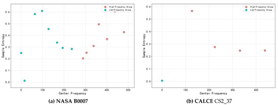
Figure 4.
K-means clustering results of IMFs in the frequency–entropy feature space for (a) NASA B0007 and (b) CALCE CS2_37.
For both batteries, K-means (K = 2) successfully separates the IMFs into two distinct groups:
Cluster 1 (LF Group): Characterized by lower center frequencies and relatively low sample entropy, this group predominantly captures the slow, monotonic trend associated with long-term capacity fade. These IMFs are highlighted in blue.
Cluster 2 (HF Group): Exhibits higher center frequencies and elevated sample entropy values, reflecting transient dynamics, abrupt fluctuations, measurement noise, and other short-term disturbances. These components are marked in red.
This clear separation confirms that the hybrid feature space (frequency + entropy) enables meaningful and physically interpretable partitioning of degradation dynamics. The resulting HF and LF signal groups are then fed into the GRU and Transformer branches, respectively, ensuring that each subnetwork processes signals aligned with its inductive bias.
3.3. Design of the Time-Series Feature Extraction Model
As illustrated in Figure 5, the proposed model adopts a parallel dual-branch architecture that integrates Transformer and GRU networks to jointly model multi-scale temporal features. The GRU branch captures high-frequency abrupt changes—such as sudden voltage drops during charging—by leveraging gated recurrent units to model local temporal dynamics. In contrast, the Transformer branch extracts low-frequency gradual trends, such as SEI layer thickening, using self-attention mechanisms and positional encoding to model long-range dependencies. The outputs from both branches are concatenated to integrate their complementary strengths, thereby enhancing the representation of complex degradation patterns. Finally, the fused features are passed through a fully connected (FC) layer for final prediction, enabling accurate modeling of both short-term fluctuations and long-term battery degradation.
3.3.1. Transformer-Based Low-Frequency Feature Extraction Branch
The input sequence is processed through multi-layer Transformer encoders for global temporal modeling. The core multi-head attention mechanism is formulated as Equation (9), which computes a weighted sum of value vectors based on query-key compatibility across multiple attention heads.
By stacking ℎ attention heads, the model effectively captures long-range dependencies and smooth low-frequency trends, such as gradual capacity fading and SEI layer growth over time. The output of the Transformer encoder is denoted as , where represents the high-dimensional feature at time step t. Finally, the temporal dimension is compressed through average pooling:
This pooled feature serves as the final embedding for subsequent prediction or classification tasks.
3.3.2. GRU-Based High-Frequency Trend Modeling Branch
A parallel multi-layer GRU network is employed to process the raw sequence XH. By leveraging gated recurrent units (GRUs), the network effectively extracts High-frequency short-term trends, such as capacity spikes and noise fluctuations. The dynamic update mechanism of the GRU is defined as follows:
The final output is the terminal state feature, which encodes the most recent temporal dynamics from the high-frequency branch.
3.3.3. Cross-Scale Feature Fusion
The dual-branch features are fused via channel-wise concatenation and fully connected layers:
The proposed architecture leverages the complementary strengths of two distinct modules: the Transformer excels in capturing long-term degradation trends—such as progressive capacity fade or increasing internal resistance, phenomena often linked to processes like SEI layer growth or lithium plating—while the GRU specializes in detecting high-frequency transient events, such as sudden voltage drops or temperature spikes during charging cycles.
This functional specialization is motivated by the inherent inductive biases of the two architectures:
Transformers, through self-attention, model global dependencies across the entire sequence, enabling effective capture of slowly evolving, cumulative degradation processes—even when separated by long temporal intervals—without suffering from vanishing gradients. In contrast, GRUs, equipped with update and reset gates, regulate information flow at each time step, making them responsive to rapid, localized dynamics. However, they are not inherently robust to noise and benefit significantly from prior signal decomposition that isolates meaningful transients from stochastic variations.
Notably, applying Transformers to high-frequency components can lead to overfitting, as the attention mechanism may attend to irrelevant fluctuations rather than true fault signatures. Conversely, GRUs struggle with long-range dependencies in low-frequency trends due to their sequential processing nature and gradient propagation limitations.
Therefore, our dual-branch design strategically assigns low-frequency components to the Transformer and high-frequency residuals to the GRU. Combined with an adaptive feature fusion mechanism, this architecture enables comprehensive, multi-scale modeling of lithium-ion battery degradation—from transient anomalies to long-term aging trends—supporting reliable health monitoring and remaining useful life prediction.

Figure 5.
Transformer-GRU Dual-Branch Network for Time-Series Feature Fusion.
4. Experimental Design and Results Analysis
4.1. Dataset
4.1.1. NASA
To validate the effectiveness of the proposed method, this study employed a lithium-ion battery aging dataset provided by the NASA Ames Prognostics Center of Excellence [40]. The dataset documents the degradation process through standardized charge–discharge experiments, which involve constant current-constant voltage (CC-CV) charging at 1.5 A up to 4.2 V, followed by discharging at 2 A until voltages reach between 2.7 V and 2.2 V.
The experimental protocol combines standard cycling with random charge–discharge cycles (Random Walk) to simulate real-world operating conditions. Time-series measurements of voltage, current, temperature, and capacity are recorded at 1 s intervals, along with electrochemical impedance spectroscopy (EIS) parameters. The experiments are terminated when the battery capacity degrades to 70–80% of its initial value, which represents the typical end-of-life threshold. All data are stored in mat format.
In this study, complete lifecycle data from batteries B0005, B0006, B0007, and B0018 were selected, and capacity degradation features were extracted for State of Health (SOH) estimation. This comprehensive setup enables an accurate evaluation of the proposed method’s ability to capture and predict battery degradation trends, reflecting its potential for real-world deployment.
4.1.2. CALCE
The second dataset used in this study is the CALCE LIB aging dataset [41,42], released by the Center for Advanced Life Cycle Engineering (CALCE) at the University of Maryland. This dataset contains cyclic aging data collected under stepped charge–discharge protocols, such as 0.5 C constant current charging to 4.2 V, followed by a rest period, and then 1 C discharging to 3.0 V. The experiments cover a wide temperature range from −20 °C to 50 °C.
In this work, four lithium-ion battery cells (CS2_35, CS2_36, CS2_37, and CS2_38) were selected from the dataset to evaluate the performance of the proposed model. A Reference Performance Test (RPT) is conducted every 50 cycles to collect detailed information on capacity, internal resistance, voltage relaxation curves, and Incremental Capacity Analysis (ICA) parameters. The experiments terminate when the battery capacity drops to 80% of its initial value or when the internal resistance increases by 30%.
The dataset is stored in both HDF5 and CSV formats, containing minute-level sampled time-series data for voltage, current, and temperature. This rich dataset provides a solid foundation for evaluating SOH estimation and Remaining Useful Life (RUL) prediction models, making it particularly suitable for advanced prognostic studies.
4.2. Experimental Parameter Settings
As shown in Table 1, the key parameters of the proposed framework include settings for the sliding window mechanism, SE-VMD decomposition, Transformer and GRU architectures, and training optimization. Below, we provide a detailed justification for their selection.

Table 1.
Hyperparameter Configuration and Roles in the Hybrid Framework for Battery Degradation.
Sliding Window Size (12, 24, 48): The window sizes are empirically selected to balance the modeling of short-term dynamics and long-term degradation trends. A window that is too small may fail to capture sufficient temporal context—particularly for LF capacity fade patterns—while an excessively large window can introduce redundant information, amplify noise, and increase the risk of overfitting [43]. The range of 12 to 48 is chosen based on domain knowledge of battery aging behavior, ensuring adequate representation of both HF fluctuations and slow, monotonic degradation trends.
Step Size: A fixed step size of 1 is adopted to maximize temporal overlap between consecutive windows. This enables dense prediction coverage, which is critical for detecting abrupt capacity drops and fine-grained degradation dynamics during battery aging.
SE-VMD Parameters (m = 2, r = 0.15 × σ): The SE-VMD method adaptively determines the optimal number of intrinsic mode functions (IMFs) using sample entropy with an embedding dimension m = 2 and a similarity tolerance = 0.15 × σ, where σ is the standard deviation of the input signal. The value r = 0.15 × σ is a widely accepted empirical choice in the sample entropy literature, particularly for mechanical degradation and physiological signals, as it provides a good trade-off between sensitivity to dynamic changes and robustness against measurement noise. Studies have shown that r values in the range 0.1σ–0.2σ yield stable entropy estimates: larger values lead to over-regularity and reduced discriminative power, whereas smaller values increase sensitivity to noise and spurious variations [44,45,46]. Similarly, m = 2 is selected based on extensive empirical evidence [47,48], as it balances the need to capture nonlinear dynamics with the constraints of finite and noisy data. For short or noisy time series—such as battery degradation data—m > 2 often results in unstable entropy estimates, while m = 1 lacks sufficient pattern discrimination and may oversimplify the signal structure.
IMF Number Constraints (kmin = 2, kmax = 12): To prevent under- or over-decomposition, the number of IMFs is constrained within a plausible range. A minimum of 2 IMFs ensures sufficient decomposition for meaningful frequency separation, while a maximum of 12 avoids generating spurious modes and excessive computational load [49].
K-means Clustering (2 clusters): The decomposed IMFs are grouped into HF and LF components using K-means clustering based on a hybrid feature set combining frequency-domain characteristics (e.g., central frequency) and sample entropy values. The number of clusters is set to 2, motivated by the bimodal nature of battery degradation signals: one cluster corresponds to the slow, monotonic capacity fade (LF trend), representing long-term aging dynamics; the other captures transient fluctuations, measurement noise, charge–discharge hysteresis, and micro-scale degradation events (HF components).This two-component decomposition aligns with established models in battery health monitoring [50], which typically describe capacity evolution as a superposition of long-term trends and short-term variations. While intermediate-frequency components or intra-class heterogeneity may exist, they are generally less dominant and difficult to distinguish consistently across diverse operating conditions and battery units. Moreover, introducing more clusters would increase model complexity without clear physical interpretability or measurable performance gain in the prediction. Therefore, binary clustering provides a physically meaningful, computationally efficient, and robust solution for separating temporal scales in degradation modeling. This design also facilitates the subsequent dual-branch architecture, where the Transformer focuses on global trend learning and the GRU captures local dynamics.
Transformer Architecture (3 layers, 4 attention heads): The Transformer encoder consists of 3 layers with 4 attention heads, a configuration commonly used in time series modeling tasks [51,52]. This setup strikes a balance between modeling capacity and training efficiency, enabling the capture of hierarchical temporal dependencies without introducing excessive complexity—particularly important given the relatively small sample sizes typical in battery degradation datasets.
GRU Hidden Units (64): The GRU network employs 64 hidden units, a widely adopted setting in sequence learning applications [53]. This configuration effectively captures short-term temporal dynamics while maintaining computational efficiency and mitigating overfitting risks.
We believe that these parameter choices are well-grounded in both empirical practice and domain-specific knowledge. While a comprehensive sensitivity analysis could offer further insights, we prioritize model interpretability, computational efficiency, and consistency with established methodologies in this application domain.
4.3. Core Experiment
4.3.1. Experimental Results
The proposed method was evaluated on four battery units from each of the NASA and CALCE datasets. For each battery, experiments were conducted using three different sliding window sizes: 12, 24, and 48. The results are visualized in Figure 6 using scatter plots that compare predicted and actual capacity degradation trajectories.
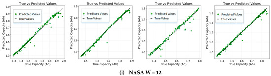
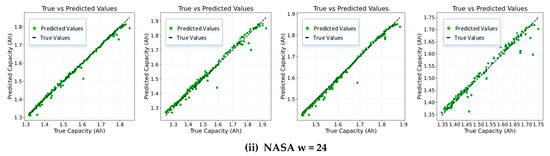
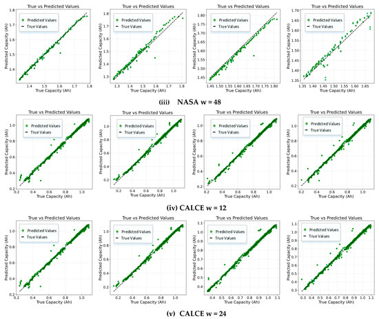
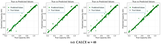
Figure 6.
Predicted vs. Actual Capacity Degradation of LIBs Using Different Sliding Window Sizes. Subfigures (i–iii): Results for batteries B0005, B0006, B0007, and B0018 from the NASA battery dataset under sliding window sizes of 12, 24, and 48, respectively. Subfigures (iv–vi): Corresponding results for batteries CS2_35, CS2_36, CS2_37, and CS2_38 from the CALCE battery dataset.
Specifically, subfigures (i), (ii), and (iii) present the results for batteries B0005, B0006, B0007, and B0018 from the NASA dataset under sliding window sizes of 12, 24, and 48, respectively. Subfigures (iv), (v), and (vi) show corresponding results for batteries CS2_35, CS2_36, CS2_37, and CS2_38 from the CALCE dataset. In Figure 6, the relationship between true and predicted capacity values is visualized. The figure shows a scatter plot comparing the true capacity degradation trajectories with the predicted ones for a given battery unit. The straight line represents the true capacity values, while the green dots indicate the predicted capacity values.
4.3.2. Discussion on the Impact of Window Size on Prediction Performance
As presented in Table 2 and Table 3, the performance of the proposed prediction framework is evaluated using the NASA and CALCE battery datasets, respectively. Both tables evaluate the model’s performance across multiple window sizes (12, 24, and 48), demonstrating its predictive capabilities under varying conditions. The evaluation metrics include the Mean Squared Error (MSE), Root Mean Squared Error (RMSE), Mean Absolute Error (MAE), Mean Absolute Percentage Error (MAPE), and the coefficient of determination (R2). These metrics are computed for multiple groups within each dataset, thereby providing insights into the model’s accuracy, reliability, and robustness.
Table 2.
Performance Metrics for the NASA Battery Dataset Across Different Window Sizes.
Table 3.
Performance Metrics for the CALCE Battery Dataset Across Different Window Sizes.
Experimental results demonstrate that the selection of sliding window length significantly affects the accuracy and stability of the prediction model, revealing how it influences the model’s ability to capture battery health states across different degradation patterns.
For the NASA dataset (Table 2), a window size of 12 achieves the lowest average MAPE of 0.6645% and the highest R2 value of 0.9822, indicating superior performance in capturing short-term fluctuations and local dynamics. This aligns well with the characteristics of the NASA dataset, which exhibits complex degradation behaviors, including sudden capacity regeneration and nonlinear fading. While larger windows (e.g., 48) show slightly improved MSE (0.000333) and RMSE (0.017686) values, they result in an increased MAPE (0.99832%) and a notable drop in R2 (0.9679). This suggests that although larger windows may reduce the impact of individual outliers—thus improving MSE and RMSE—they also introduce redundant or irrelevant historical information that hinders the model’s responsiveness to rapid changes. Therefore, shorter windows are more suitable for capturing transient variations in highly dynamic degradation processes.
In contrast, the CALCE dataset (Table 3) demonstrates relatively stable performance across all window sizes. The best average MAPE of 1.2382% is achieved with a window size of 24, while the R2 remains consistently above 0.9945. These results reflect the smoother and more trend-driven degradation behavior of CALCE batteries. Increasing the window size allows the model to better capture long-term patterns without significantly sacrificing accuracy, as evidenced by the stable R2 values and only marginal increases in MAPE for window sizes up to 24. However, at window size 48, both MAPE and RMSE show noticeable deterioration, suggesting that excessively large windows may introduce outdated or irrelevant information, which can distort short-term dynamics and degrade prediction accuracy. This indicates that while larger windows can enhance pattern extraction in trend-dominated datasets, an optimal balance must be struck to avoid over-smoothing and loss of responsiveness.
In summary, the optimal window length selection should be guided by the inherent characteristics of battery degradation dynamics, as demonstrated by this study. For datasets exhibiting nonlinear and fluctuating degradation patterns (e.g., NASA), smaller window sizes (e.g., 12 steps) are critical for enhancing the model’s sensitivity to short-term variations and mitigating the risk of over-smoothing in noisy or adversarial scenarios. Conversely, for datasets with stable and trend-dominated degradation profiles (e.g., CALCE), moderately increasing the window size (e.g., up to 24 steps) enables the model to capture global degradation trends while maintaining robustness against local perturbations. However, excessively large windows (e.g., 48 steps) may introduce outdated or irrelevant information, degrading performance and reducing adaptability to dynamic operational conditions. This work establishes a data-driven adaptation framework that dynamically balances short-term responsiveness and long-term pattern extraction, thereby enhancing the AI security system’s robustness under adversarial noise and generalization across heterogeneous datasets.
4.3.3. Comparison with Other Experimental Methods
Furthermore, using a window size of 24 as an example, we compare the proposed method with baseline experiments, including models such as LSTM and Transformer. The performance metrics—MSE, RMSE, MAE, MAPE, and R2—of each experiment relative to the primary experiment are summarized in Table 4 and Table 5. These tables provide a detailed comparison of the predictive accuracy among the different methods. To facilitate an intuitive evaluation of model performance, we present an overall comparison across all metrics using radar charts, as shown in Figure 7. For visualization consistency, the R2 metric was transformed using 1−R2, and all metrics were normalized to a [0, 1] scale to ensure uniformity. This graphical analysis enables a clear interpretation of the relative strengths and limitations of each model, further highlighting the superior precision and robustness of the proposed framework.
Table 4.
Performance Metrics for Different Models on the NASA Battery Dataset with Window Size = 24.
Table 5.
Performance Metrics for Different Models on the CALCE Battery Dataset with Window Size = 24.
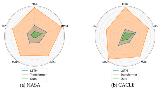
Figure 7.
Radar Chart Comparison of Performance Metrics for Different Models on (a) NASA and (b) CALCE Battery Datasets.
To validate the degradation prognostic performance of the proposed method for LIBs, comparative experiments were conducted on two benchmark datasets: NASA and CALCE battery degradation dataset. The proposed SE-VMD-based hybrid framework was implemented by decomposing the capacity signal into HF and LF components via SE-VMD. These components were subsequently processed by Transformer and Gated Recurrent Unit (GRU) networks, respectively, followed by frequency-aware feature fusion. The results were benchmarked against conventional models, including standalone LSTM and Transformer networks, to evaluate the effectiveness of the multi-scale temporal modeling strategy in capturing both abrupt anomalies and gradual degradation trends.
From the experimental results on the NASA dataset (Table 4), the proposed method significantly outperforms the baseline models across all evaluation metrics. Specifically, the average MSE is 0.000397, representing a 23.1% reduction compared to LSTM (0.000515) and a 55.1% improvement over the Transformer (0.000885). The average MAPE reaches 0.7047%, showing a 21.3% decrease compared to LSTM (0.8956%) and a 47.9% decrease compared to Transformer (1.3526%). Additionally, the mean R2 value achieves 0.9804, demonstrating superior overall fitting performance.
The performance on the CALCE dataset further confirms the robustness and generalization capability of the proposed approach. As shown in Table 5, the proposed method consistently surpasses both LSTM and Transformer across all metrics. It achieves an average MAPE of 1.2382%, lower than that of LSTM (1.4719%) and Transformer (2.1604%), while maintaining an average R2 above 0.9945, reflecting stronger trend modeling ability. Particularly in GROUP CS2_37, the proposed method achieves a remarkably low MAPE of 0.9299%, significantly outperforming the other models and highlighting its better adaptability to slow and regular aging processes.
The proposed dual-branch architecture enhances AI security systems by robustly handling heterogeneous degradation patterns through parallel processing of HF and LF components in battery capacity signals. High-frequency components, which capture abrupt fluctuations and anomalies (e.g., sudden capacity drops in NASA datasets), are modeled by the Gated Recurrent Unit (GRU) to efficiently learn local temporal dynamics under uncertain operational conditions. Meanwhile, low-frequency components, representing gradual degradation trends (e.g., stable aging in CALCE datasets), are processed by the Transformer to leverage its superior long-range dependency modeling for global pattern extraction. This dual-branch strategy enables multi-scale temporal modeling, effectively adapting to both complex signals in dynamic environments (NASA) and stable trends in controlled scenarios (CALCE). The design further improves system robustness by isolating high-frequency noise from critical degradation trends, reducing vulnerability to adversarial perturbations. While the SE-VMD-based decomposition is validated in ablation studies, the dual-branch framework itself demonstrates strong generalization across heterogeneous datasets and resilience to input variability.
4.4. Ablation Study on Signal Decomposition Methods
To evaluate the effectiveness of the proposed sample entropy-guided VMD (SE-VMD) and its role in degradation prognostics for LIBs, an ablation study was conducted by comparing three configurations: (1) No decomposition (raw data fed directly into the model), (2) Traditional VMD, and (3) SE-VMD. Experiments were performed on two benchmark datasets—NASA (B0005, B0006, B0007, B0018) and CALCE (CS2_35,CS2_36,CS2_37,CS2_38)—with results summarized in Table 6.
Table 6.
Comparison of RMSE for Prediction Accuracy with and without VMD-Based Signal Decomposition on NASA and CALCE Battery Datasets.
As shown in Table 6, the SE-VMD achieves the lowest RMSE values across all battery units in both datasets, outperforming both the baseline (no decomposition) and traditional VMD. For instance, in the NASA dataset, the average RMSE for the improved VMD is 0.0176, compared to 0.0347 (traditional VMD) and 0.0432(no decomposition)—a 59.2% reduction relative to the baseline. Similarly, in the CALCE dataset, the improved VMD reduces the average RMSE from 0.0657 (no decomposition) to 0.0151 (improved VMD), a 77.1% improvement. These results demonstrate that the adaptive IMF selection and frequency-based separation in the improved VMD significantly enhance noise suppression and multi-scale feature extraction.
Notably, the no-decomposition method struggles with complex degradation patterns. In the NASA dataset, B0007 exhibits the highest RMSE (0.0818), likely due to its nonlinear capacity regeneration behavior, which confounds direct modeling of raw signals. Similarly, CS2_36 in the CALCE dataset shows a relatively high RMSE (0.0718), underscoring the limitations of unprocessed data in capturing subtle long-term trends. In contrast, SE-VMD effectively isolates transient fluctuations (processed by GRUs) and gradual degradation (modeled by Transformers), enabling robust prediction even in challenging scenarios.
To further illustrate the performance differences, Figure 8 presents boxplots comparing RMSE distributions across all experiments. The results reveal:
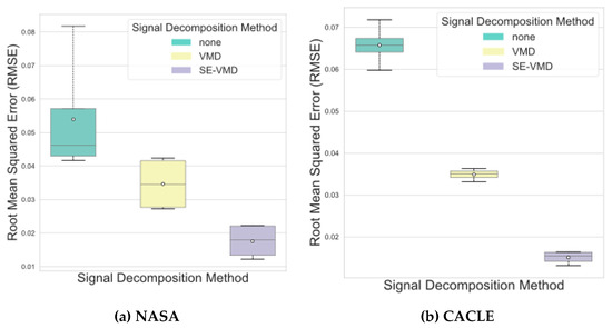
Figure 8.
Comparison of Root Mean Squared Error (RMSE) with and without VMD-Based Signal Decomposition on (a) NASA and (b) CALCE Battery Datasets.
- (1)
- SE-VMD exhibits the narrowest interquartile range (IQR) and the lowest median RMSE, indicating minimal variance and higher stability.
- (2)
- Traditional VMD shows moderate performance, but its IQR is wider than SE-VMD, with some outliers, suggesting limited adaptability to complex patterns.
- (3)
- The no-decomposition method has the widest IQR and highest median RMSE, reflecting significant variability and instability, particularly in datasets with abrupt degradation (e.g., NASA-B0007).
The boxplots demonstrate that the SE-VMD framework reduces prediction errors and ensures consistent performance across heterogeneous aging patterns. This is achieved by combining sample entropy (SE)-guided IMF selection, which dynamically selects robust IMFs to minimize dataset-specific overfitting and enhance cross-dataset generalization, with K-means clustering-based frequency separation, which isolates high-frequency noise from low-frequency degradation trends to improve adversarial robustness. Together, these components strengthen the AI system’s ability to handle dynamic operational conditions and security threats, establishing a secure preprocessing pipeline for reliable degradation modeling in safety-critical applications such as battery health monitoring.
4.5. Computational Efficiency Analysis
To evaluate the computational overhead introduced by the proposed SE-VMD-based decomposition, we compare the runtime performance of three configurations: (1) no decomposition, (2) traditional VMD, and (3) SE-VMD. All experiments are conducted under identical hardware conditions, and the model architectures after decomposition remain consistent.
As shown in Table 7, the decomposition step introduces notable computational costs. Traditional VMD adds 94.59 s of preprocessing time, while SE-VMD significantly increases decomposition time to 613.61 s—over six times longer than VMD. This substantial increase is due to the iterative entropy computation and adaptive mode selection process inherent in SE-VMD, which enhances feature quality at the expense of computational efficiency.
Table 7.
Computational Efficiency Comparison.
Despite the longer decomposition time, this step is performed offline and only once per battery unit, as degradation analysis typically operates on batch-processed historical data. This makes SE-VMD feasible for long-term battery health monitoring systems where predictions are made over extended operational cycles.
Interestingly, the increased decomposition complexity does not negatively impact subsequent model training or inference. Training time per epoch varies slightly across methods, from 2.52 s (VMD) to 3.50 s (SE-VMD), with the baseline at 3.32 s. Inference latency remains extremely low and stable, ranging from 0.0146 ms to 0.0199 ms, indicating that the neural network components operate efficiently regardless of the decomposition strategy.
However, the total pipeline time—encompassing decomposition, multi-epoch training, and inference—is significantly higher for SE-VMD (838.2 s) compared to VMD (219 s) and the baseline (123.6 s), primarily due to the prolonged preprocessing phase.
These results demonstrate that while SE-VMD incurs a high upfront computational cost, it enables richer signal representations. Therefore, its use is justified in accuracy-critical applications where decomposition can be treated as a one-time offline procedure.
5. Conclusions and Future Work
This study proposes a secure and robust framework for LIB capacity prediction by integrating a dual-branch architecture (combining Gated Recurrent Units for short-term fluctuations and Transformers for long-term trends) with sample entropy-guided SE-VMD-based adaptive signal decomposition. The framework enhances resilience to adversarial noise and generalization across heterogeneous degradation patterns through multi-scale modeling and frequency-aware feature fusion. Experimental validation on NASA and CALCE datasets demonstrates superior accuracy, stability, and interpretability, particularly in safety-critical scenarios where reliable risk detection is paramount.
Integrating domain knowledge into data-driven frameworks improves generalization and trustworthiness in safety-critical applications [54], a principle that motivates our ongoing efforts to enhance model interpretability and physical consistency. Future work will prioritize optimizing decomposition efficiency by applying lightweight algorithms, integrating battery physics-based constraints to improve interpretability, and developing online adaptive mechanisms to dynamically adjust model weights in response to environmental shifts or data anomalies. Additionally, advanced feature learning strategies—such as attention-based fusion or hierarchical gating networks—will be explored to further refine the integration of multi-scale representations, thereby ensuring real-time reliability in safety-critical systems. However, the computational overhead introduced by SE-VMD poses latency risks in real-time applications.
Author Contributions
Conceptualization: Y.L., J.Z. and B.Z. Methodology: Y.L. Software: Q.L. Validation: Q.L. Formal Analysis: Y.L. Investigation: Y.L. Resources: B.Z. Data Curation: B.Z. Writing—Original Draft Preparation: Y.L. Writing—Review and Editing: J.G. Visualization: Q.L. Supervision: J.Z. Project Administration: J.Z. Funding Acquisition: J.Z. All authors have read and agreed to the published version of the manuscript.
Funding
This research was supported by multiple funding sources: The Municipal Government of Quzhou (Grant Nos. 2023D015, 2023D014, 2023D033, 2023D034, and 2023D035); The Tianjin Science and Technology Program Projects (Grant No. 24YDTPJC00630); The Tianjin Municipal Education Commission Research Program Project (Grant No. 2022KJ012); The Teaching Reform Project of Tianjin Normal University (Grant No. JGZD01218010); The 2025 Innovation and Entrepreneurship Training Program for College Students (Grant No. 202510065114).
Data Availability Statement
The data supporting the findings of this study are available. The NASA dataset used in this study is publicly available and can be accessed at NASA Battery Data Set URL (https://phm-datasets.s3.amazonaws.com/NASA/5.+Battery+Data+Set.zip (accessed on 17 May 2025)).
Acknowledgments
The authors wish to acknowledge the support of all team members and institutions involved in this research. No additional specific acknowledgments are necessary.
Conflicts of Interest
The authors declare no conflicts of interest.
CALCE dataset
The CALCE battery dataset utilized in this research is also publicly accessible and can be downloaded from CALCE Battery Data Set URL (https://calce.umd.edu/battery-dataset (accessed on 17 May 2025)).
References
- Nekahi, A.; Reddy, A.K.M.R.; Li, X.; Deng, S.; Zaghib, K. Rechargeable Batteries for the Electrification of Society: Past, Present, and Future. Electrochem. Energy Rev. 2025, 8, 1–30. [Google Scholar]
- Gharehghani, A.; Rabiei, M.; Mehranfar, S.; Saeedipour, S.; Andwari, A.M.; García, A.; Reche, C.M. Progress in Battery Thermal Management Systems Technologies for Electric Vehicles. Renew. Sustain. Energy Rev. 2024, 202, 114654. [Google Scholar] [CrossRef]
- Bokkassam, S.D.; Krishnan, J.N. Lithium Ion Batteries: Characteristics, Recycling and Deep-Sea Mining. Battery Energy 2024, 3, 20240022. [Google Scholar]
- Frost, S.; Welford, R.; Cheung, D. CSR Asia News Review: October–December 2006. Corp. Soc. Responsib. Environ. Manag. 2007, 14, 52–59. [Google Scholar] [CrossRef]
- Baird, A.R.; Archibald, E.J.; Marr, K.C.; Ezekoye, O.A. Explosion hazards from lithium-ion battery vent gas. J. Power Sources 2020, 446, 227257. [Google Scholar] [CrossRef]
- Rezvanizaniani, S.M.; Liu, Z.; Chen, Y.; Lee, J. Review and recent advances in battery health monitoring and prognostics technologies for electric vehicle (EV) safety and mobility. J. Power Sources 2014, 256, 110–124. [Google Scholar] [CrossRef]
- Zhou, B.; Cheng, C.; Ma, G.; Zhang, Y. Remaining useful life prediction of lithium-ion battery based on attention mechanism with positional encoding. IOP Conf. Ser. Mater. Sci. Eng. 2020, 895, 012006. [Google Scholar] [CrossRef]
- Guo, W.; Sun, Z.; Vilsen, S.B.; Meng, J.; Stroe, D.I. Review of “grey box” lifetime modeling for lithium-ion battery: Combining physics and data-driven methods. J. Energy Storage 2022, 56, 105992. [Google Scholar] [CrossRef]
- Li, D.; Yang, L.; Li, C. Control-oriented thermal-electrochemical modeling and validation of large size prismatic lithium battery for commercial applications. Energy 2021, 214, 119057. [Google Scholar] [CrossRef]
- Chen, N.; Zhang, P.; Dai, J.; Gui, W. Estimating the state-of-charge of lithium-ion battery using an H-infinity observer based on electrochemical impedance model. IEEE Access 2020, 99, 1. [Google Scholar] [CrossRef]
- Zhang, C.; Allafi, W.; Dinh, Q.; Ascencio, P.; Marco, J. Online estimation of battery equivalent circuit model parameters and state of charge using decoupled least squares technique. Energy 2018, 142, 678–688. [Google Scholar] [CrossRef]
- Naseri, F.; Schaltz, E.; Stroe, D.-I.; Gismero, A.; Farjah, E. An enhanced equivalent circuit model with real-time parameter identification for battery state-of-charge estimation. IEEE Trans. Ind. Electron. 2022, 69, 3743–3751. [Google Scholar] [CrossRef]
- Zhang, C.; He, Y.; Yuan, L.; Xiang, S.; Wang, J. Prognostics of Lithium-Ion Batteries Based on Wavelet Denoising and DE-RVM. Comput. Intell. Neurosci. 2015, 2015, 14. [Google Scholar] [CrossRef] [PubMed]
- Wei, M.; Ye, M.; Zhang, C.; Wang, Q.; Lian, G.; Xia, B. Integrating Mechanism and Machine Learning Based Capacity Estimation for LiFePO4 Batteries Under Slight Overcharge Cycling. Energy 2024, 296, 131208. [Google Scholar] [CrossRef]
- Kim, S.; Lee, P.-Y.; Lee, M.; Kim, J.; Na, W. Improved state-of-health prediction based on auto-regressive integrated moving average with exogenous variables model in overcoming battery degradation-dependent internal parameter variation. J. Energy Storage 2022, 46, 103888. [Google Scholar] [CrossRef]
- Wang, Z.; Shangguan, W.; Peng, C.; Meng, Y.; Chai, L.; Cai, B. A Predictive Maintenance Strategy for a Single Device Based on Remaining Useful Life Prediction Information: A Case Study on Railway Gyroscope. IEEE Trans. Instrum. Meas. 2024, 73, 1–14. [Google Scholar] [CrossRef]
- Liu, Z.; He, H.; Xie, J.; Wang, K.; Huang, W. Self-discharge prediction method for lithium-ion batteries based on improved support vector machine. J. Energy Storage 2022, 55, 105571. [Google Scholar] [CrossRef]
- Zhang, Y.; Xiong, R.; He, H.; Pecht, M.G. Long short-term memory recurrent neural network for remaining useful life prediction of lithiumion batteries. IEEE Trans. Veh. Technol. 2018, 67, 5695–5705. [Google Scholar] [CrossRef]
- Zheng, S.; Ristovski, K.; Farahat, A.; Gupta, C. Long short-term memory network for remaining useful life estimation. In Proceedings of the 2017 IEEE International Conference on Prognostics and Health Management (ICPHM), Piscataway, NJ, USA, 19–21 June 2017; IEEE: New York, NY, USA, 2017; pp. 88–95. [Google Scholar]
- Gugulothu, N.; Tv, V.; Malhotra, P.; Vig, L.; Agarwal, P.; Shroff, G. Predicting remaining useful life using time series embeddings based on recurrent neural networks. Int. J. Progn. Health Manag. 2018, 9, 1–10. [Google Scholar] [CrossRef]
- Catelani, M.; Ciani, L.; Fantacci, R.; Patrizi, G.; Picano, B. Remaining useful life estimation for prognostics of lithium-ion batteries based on recurrent neural network. IEEE Trans. Instrum. Meas. 2021, 70, 1–11. [Google Scholar] [CrossRef]
- Khalid, A.; Sundararajan, A.; Acharya, I.; Sarwat, A.I. Prediction of liion battery state of charge using multilayer perceptron and long short-term memory models. In Proceedings of the 2019 IEEE Transportation Electrification Conference and Expo (ITEC), Detroit, MI, USA, 19–21 June 2019; IEEE: New York, NY, USA, 2019; pp. 1–6. [Google Scholar]
- Mo, Y.; Wu, Q.; Li, X.; Huang, B. Remaining useful life prediction of lithium-ion battery based on AConvST-LSTM-Net-TL. Phys. Scr. 2025, 100, 026010. [Google Scholar] [CrossRef]
- Mo, Y.; Wu, Q.; Li, X.; Huang, B. Remaining useful life estimation via transformer encoder enhanced by a gated convolutional unit. J. Intell. Manuf. 2021, 32, 1997–2006. [Google Scholar] [CrossRef]
- Jha, A.; Dorkar, O.; Biswas, A.; Emadi, A. iTransformer Network Based Approach for Accurate Remaining Useful Life Prediction in Lithium-Ion Batteries. In Proceedings of the 2024 IEEE Transportation Electrification Conference and Expo (ITEC), Chicago, IL, USA, 19–21 June 2024. [Google Scholar] [CrossRef]
- Yang, J.; Wang, X.; Zhang, M.; Jiang, L. Bayesian Meta Random Graph Implicit Enhanced Network for Lithium-Ion Batteries Remaining Useful Life Prediction With Few-Shot and Uncertainty Interference. IEEE Trans. Transport. Electrific. 2025, 11, 9877. [Google Scholar] [CrossRef]
- Chen, C.; Chen, H.; Shi, J.; Yue, D.; Shi, G.; Lyu, D. Estimating Lithium-Ion Battery Health Status: A Temporal Deep Learning Approach With Uncertainty Representation. IEEE Sens. J. 2025, 25, 26931–26948. [Google Scholar] [CrossRef]
- Chen, C.; Tao, G.; Shi, J.; Shen, M.; Zhu, Z.H. A Lithium-Ion Battery Degradation Prediction Model With Uncertainty Quantification for Its Predictive Maintenance. IEEE Trans. Ind. Electron. 2024, 71, 3650–3659. [Google Scholar] [CrossRef]
- Ren, L.; Dong, J.; Wang, X.; Meng, Z.; Zhao, L.; Deen, M.J. A Data-Driven Auto-CNN-LSTM Prediction Model for Lithium-Ion Battery Remaining Useful Life. IEEE Trans. Ind. Inform. 2021, 17, 3478–3487. [Google Scholar] [CrossRef]
- Shen, L.; Li, J.; Zuo, L.; Zhu, L.; Shen, H.T. Source-free cross-domain state of charge estimation of lithium-ion batteries at different ambient temperatures. IEEE Trans. Power Electron. 2023, 38, 6851–6862. [Google Scholar] [CrossRef]
- Wei, Y.; Wu, D. Prediction of state of health and remaining useful life of lithium-ion battery using graph convolutional network with dual attention mechanisms. Reliab. Eng. Syst. Saf. 2023, 230, 108947. [Google Scholar] [CrossRef]
- Tong, A.; Zhang, J.; Xie, L. Intelligent Fault Diagnosis of Rolling Bearing Based on Gramian Angular Difference Field and Improved Dual Attention Residual Network. Sensors 2024, 24, 2156. [Google Scholar] [CrossRef]
- Cai, Y.; Li, W.; Zahid, T.; Zheng, C.; Zhang, Q.; Xu, K. Early prediction of remaining useful life for lithium-ion batteries based on CEEMDAN-transformer-DNN hybrid model. Heliyon 2023, 9, 13. [Google Scholar] [CrossRef]
- Wu, M.; Yue, C.; Zhang, F.; Li, J.; Huang, W.; Hu, S.; Tang, J. A combined GRU-MLR method for predicting the remaining useful life of lithium batteries under multiscale decomposition. Energy Storage Sci. Technol. 2023, 12, 2220. [Google Scholar]
- Liu, Y.; Han, L.; Wang, Y.; Zhu, J.; Zhang, B.; Guo, J. An Evolutionary Deep Learning Framework for Accurate Remaining Capacity Prediction in Lithium-Ion Batteries. Electronics 2025, 14, 400. [Google Scholar] [CrossRef]
- Colominas, M.A.; Schlotthauer, G.; Torres, M.E. Improved Complete Ensemble EMD: A Suitable Tool for Biomedical Signal Processing. Biomed. Signal Process. Control 2014, 14, 19–29. [Google Scholar] [CrossRef]
- Wu, Z.; Huang, N.E. Ensemble empirical mode decomposition: A noise-assisted data analysis method. Adv. Adapt. Data Anal. 2009, 1, 1–41. [Google Scholar] [CrossRef]
- Wang, R.; Hou, Q.L.; Shi, R.Y.; Zhou, Y.X.; Hu, X. Remaining useful life prediction method of lithium battery based on variational mode decomposition and integrated deep model. Chin. J. Sci. Instrum. 2021, 42, 111–120. [Google Scholar]
- Dragomiretskiy, K.; Zosso, D. Variational Mode Decomposition. IEEE Trans. Signal Process. 2014, 62, 531–544. [Google Scholar] [CrossRef]
- Bhaskar, S.; Kai, G. Battery Data Set. In NASA AMES Prognostics Data Repository; NASA Ames Research Center: Moffett Field, CA, USA, 2007. [Google Scholar]
- CALCE Battery Group. CALCE Lithium-Ion Battery Aging Dataset. University of Maryland. 2020. Available online: http://calce.umd.edu/battery-data (accessed on 22 September 2025).
- Zhou, X. Open-Source Code and Preprocessed CALCE Dataset for Battery Prognostics. GitHub Repository. 2021. Available online: https://github.com/XiuzeZhou/CALCE (accessed on 22 September 2025).
- Lim, B.; Arık, S.Ö.; Loeff, N.; Pfister, T. Temporal fusion transformers for interpretable multi-horizon time series forecasting. Int. J. Forecast. 2021, 37, 1325–1338. [Google Scholar] [CrossRef]
- Richman, J.S.; Moorman, J.R. Physiological time-series analysis using approximate entropy and sample entropy. Am. J. Physiol. Heart Circ. Physiol. 2000, 278, H2039–H2049. [Google Scholar] [CrossRef] [PubMed]
- Lake, D.E.; Richman, J.S.; Griffin, M.P.; Moorman, J.R. Sample entropy analysis of neonatal heart rate variability. Am. J. Physiol. Regul. Integr. Comp. Physiol. 2002, 283, R789. [Google Scholar] [CrossRef]
- Yentes, J.M.; Hunt, N.; Schmid, K.K.; Kaipust, J.P.; McGrath, D.; Stergiou, N. The Appropriate Use of Approximate Entropy and Sample Entropy with Short Data Sets. Ann. Biomed. Eng. 2013, 41, 349–365. [Google Scholar] [CrossRef]
- Costa, M.; Goldberger, A.L.; Peng, C.K. Multiscale entropy analysis of biological signals. Phys. Rev. E Stat. Nonlinear Soft Matter Phys. 2005, 71, 021906. [Google Scholar] [CrossRef] [PubMed]
- Xu, W.; Li, Y.; Yang, B. Prediction for Remaining Useful Life of Lithium-ion Batteries Based on NGO-VMD and LSTM. In Proceedings of the 2024 Prognostics and System Health Management Conference (PHM), Stockholm, Sweden, 28–31 May 2024. [Google Scholar] [CrossRef]
- Lei, Y.; Liu, L.; Bai, W.-L.; Feng, H.-X.; Wang, Z.-Y. Seismic Signal Analysis Based on Adaptive Variational Mode Decomposition for High-speed Rail Seismic Waves. Appl. Geophys. Bull. Chin. Geophys. Soc. 2024, 21, 358–371. [Google Scholar] [CrossRef]
- Liu, D.; Pang, J.; Zhou, J.; Peng, Y.; Pecht, M. Prognostics for state of health estimation of lithium-ion batteries based on combination Gaussian process functional regression. Microelectron. Reliab. 2013, 53, 832–839. [Google Scholar] [CrossRef]
- Zhou, H.; Zhang, S.; Peng, J.; Zhang, S.; Li, J.; Xiong, H.; Zhang, W. Informer: Beyond Efficient Transformer for Long Sequence Time-Series Forecasting. Proc. AAAI Conf. Artif. Intell. 2020, 35, 11106–11115. [Google Scholar] [CrossRef]
- Wu, H.; Xu, J.; Wang, J.; Long, M. Autoformer: Decomposition Transformers with Auto-Correlation Long-Term Series Forecasting. Adv. Neural Inf. Process. Syst. 2021, 34, 22419–22430. [Google Scholar] [CrossRef]
- Wu, H.; Xu, J.; Wang, J.; Long, M. A hybrid deep learning approach for remaining useful life prediction of lithium-ion batteries based on discharging fragments. Appl. Energy 2024, 358, 122555. [Google Scholar] [CrossRef]
- Wang, Q.; Chen, L.; Xiao, G.; Wang, P.; Gu, Y.; Lu, J. Elevator fault diagnosis based on digital twin and PINNs-e-RGCN. Sci. Rep. 2024, 14, 3071. [Google Scholar] [CrossRef] [PubMed]
Disclaimer/Publisher’s Note: The statements, opinions and data contained in all publications are solely those of the individual author(s) and contributor(s) and not of MDPI and/or the editor(s). MDPI and/or the editor(s) disclaim responsibility for any injury to people or property resulting from any ideas, methods, instructions or products referred to in the content. |
© 2025 by the authors. Licensee MDPI, Basel, Switzerland. This article is an open access article distributed under the terms and conditions of the Creative Commons Attribution (CC BY) license (https://creativecommons.org/licenses/by/4.0/).