Deep Learning System for Speech Command Recognition

Abstract

We present a deep learning model for the recognition of speech commands in the English language. The dataset is based on the Google Speech Commands Dataset by Warden P., version 0.01, and it consists of ten distinct commands (“left”, “right”, “go”, “stop”, “up”, “down”, “on”, “off”, “yes”, and “no”) along with additional “silence” and “unknown” classes. The dataset is split in a speaker-independent manner, with 70% of speakers assigned to the training set and 15% to the test set and validation set. All audio clips are sampled at 16 kHz, with a total of 46 146 clips. Audio files are converted into Mel spectrogram representations, which are then used as input to a deep learning model composed of a four-layer convolutional neural network followed by two fully connected layers. The model employs Rectified Linear Unit (ReLU) activation, the Adam optimizer, and dropout regularization to improve generalization. The achieved testing accuracy is 96.05%. Micro- and macro-averaged precision, recall, and F1-score of 95% are reported to reflect class-wise performance, and a confusion matrix is also provided. The proposed model has been deployed on a Raspberry Pi 5 as a Fog computing device for real-time speech recognition applications.

1. Introduction

With the rapid development of deep learning systems, speech recognition has become a widely adopted technology in modern computer science. In this paper, we present a deep learning-based system for the recognition of spoken commands in the English language. The task involves ten commands (“left”, “right”, “go”, “stop”, “up”, “down”, “on”, “off”, “yes”, and “no”), extended with two auxiliary classes: “silence” and “unknown”. The dataset used is an improved version of the Google Speech Commands dataset [1].

The proposed system consists of a Convolutional Neural Network (CNN) followed by a fully connected neural network serving as the classification head. Input audio files are first converted into Mel spectrograms, which the CNN processes to extract discriminative features. These features are then forwarded to the classification head for final prediction.

The trained model is deployed on a Raspberry Pi 5 within a Fog computing setup. A dedicated application records spoken commands through a microphone, generates Mel spectrograms, and outputs the top three predicted commands in real time. This setup illustrates a practical and efficient approach for embedded speech recognition.

The main contributions of this work are:

• The implementation of a CNN-based model for embedded real-time speech recognition on a Raspberry Pi 5.
• The integration of Mel spectrograms with a CNN architecture for accurate classification of both standard commands and additional “silence” and “unknown” classes.
• A lightweight and efficient real-time processing pipeline for audio capture, feature extraction, and top-3 prediction suitable for Fog and edge devices.

The rest of this paper is structured as follows: Section 2 reviews related work on Mel spectrograms and CNNs in speech recognition. Section 3 introduces the theoretical background of Mel spectrograms in speech analysis. Section 4 discusses the role and significance of CNNs in this task. Section 5 details the system architecture and implementation. Section 6 presents the experimental results and discussion, and Section 7 concludes the paper.

2. Related Work

To date, research has demonstrated remarkable scientific achievements in the areas of speech recognition, voice command interpretation, and speech signal processing across various contexts. Researchers have defined certain benchmark standards that are widely accepted and difficult to surpass, leading to the use of specific methods and algorithms not only in this study but also in many other scientific investigations. Related work is organized in five sections.

2.1. Classical Baselines for Keyword Spotting and Audio Classification

Early work on small-footprint keyword spotting employed convolutional neural networks (CNNs), which achieved good accuracy with low computational cost [2,3,4]. Later, optimized variants such as DS-CNN [5] established strong baselines on the Google Speech Commands dataset [6,7]. More recent models, including TinySpeech [8] and EdgeSpeechNet [9], further explored the accuracy–efficiency trade-off for real-time applications. In addition, CNN-based methods have been applied to audio interval retrieval, demonstrating effective extraction of temporal audio segments for classification tasks [10].

2.2. Transfer Learning Approaches

Recent advances in audio classification have increasingly leveraged transfer learning from large-scale pretrained models. For example, CNNs pretrained on the AudioSet dataset have shown strong performance [11]. Wav2vec 2.0, a self-supervised framework for general-purpose speech representations, was introduced in [12]. Similarly, universal non-semantic speech representations transferable across diverse tasks have been explored in [13,14].

2.3. Attention and Conformer Architectures

Attention-based models have transformed speech recognition and keyword spotting. The Conformer architecture, combining convolutional and transformer layers, has set a new state-of-the-art in automatic speech recognition by capturing both local and global dependencies [15]. Other attention-based variants, such as ContextNet [16], demonstrate improved robustness by incorporating global context into CNNs. These architectures provide promising directions for building accurate yet efficient audio models.

2.4. Tiny Models and Efficiency-Focused Baselines

In the context of tiny models and efficiency-focused baselines, recent research has emphasized the development of compact neural networks for keyword spotting on embedded devices. Efficient dilated convolutional architectures have been proposed that achieve small-footprint KWS [17], providing a strong baseline for edge applications. Similarly, lightweight CNN models optimized for energy- and memory-constrained environments have also been investigated [18], demonstrating practical strategies for deployment under strict resource limitations. Further contributions highlight additional efficiency-focused approaches, including single-word recognition with improved out-of-distribution detection [2] and quantized CNN models [19], reinforcing the effectiveness of tiny models for real-world embedded scenarios. Collectively, these studies offer a comprehensive set of baselines and design principles for implementing high-performance, resource-efficient KWS systems.

2.5. Noise Robustness and Out-of-Distribution Handling (OOD)

Noise robustness and out-of-distribution handling remain critical challenges in speech command recognition. Recent studies have explored multiple strategies to improve resilience under noisy conditions and unseen data distributions. Noise-aware training and data augmentation with reverberant and background noise can significantly enhance robustness to real-world audio variations [20,21]. Domain generalization techniques have been proposed to adapt models to diverse data distributions, achieving better performance on OOD inputs [22]. Additionally, frameworks leveraging uncertainty modeling and feature augmentation have further strengthened OOD generalization, maintaining high recognition accuracy across heterogeneous acoustic environments [23,24]. Collectively, these approaches provide a comprehensive set of strategies for developing speech recognition systems that are robust to noise while capable of effective OOD generalization.

3. Mel Spectrograms in Speech Recognition

Mel spectrograms are fundamental components in contemporary speech recognition technologies because they represent audio signals in a manner that closely matches human hearing. In contrast to linear spectrograms, Mel spectrograms use a nonlinear frequency scaling that highlights lower frequency bands, where the majority of speech-related information is concentrated. This scaling relies on the Mel scale, which models the way the human ear perceives different sound frequencies [25].

A Mel spectrogram represents audio in the time-frequency domain, with the frequency axis adjusted according to the Mel scale—a perceptual scale designed to reflect the human ear’s sensitivity to pitch. This transformation converts linear frequency values into the Mel scale, placing greater emphasis on the frequency ranges that are more prominent in human auditory perception. For instance, the conversion typically follows this relationship [25,26]:

$$Mel(f)=2595 {log}_{10}(1+{\displaystyle \frac{f}{700}}),$$

(1)

where f is the frequency in Hz.

The Mel spectrum is derived by applying the short-time Fourier transform (STFT) to each frame of the audio signal, converting the linear frequency scale into the perceptually motivated logarithmic Mel scale [27]. Subsequently, the signal passes through a filter bank, resulting in a set of features often interpreted as eigenvectors. These features effectively represent the distribution of signal energy across the Mel-scale frequencies. The number of Mel frequency channels determines the frequency resolution of the Mel spectrogram. In this study, we use 64 Mel filter banks, which is a widely adopted choice in many speech and audio classification tasks (it can be 40, 64, 128 in some studies [27,28]). This number strikes a balance between capturing sufficient spectral detail and maintaining computational efficiency [27]. Fewer Mel bands may lead to loss of relevant frequency information, while a significantly higher number could increase the dimensionality and computational cost without a proportional gain in performance. The selection of 64 Mel bands provides a compact yet informative representation of the audio signal, particularly suitable for deep learning models [27,28].

Specifically, Mel filter banks approximate the frequency resolution of the human auditory system [29,30], emphasizing low- and mid-frequency bands that carry discriminative cues in speech and environmental sounds. Compared to STFT, Mel spectrograms provide a perceptually motivated frequency scaling; compared to wavelet and Gabor transforms, they are computationally more efficient and widely standardized in speech and audio processing [31,32,33,34].

Table 1. Trade-offs between STFT, Wavelet, Gabor, and Mel Spectrograms.

Method	Characteristics	Limitations	Advantages of Mel
STFT	Linear frequency resolution, widely used in spectral analysis	Equal weight to all frequencies; does not reflect human auditory perception	Mel emphasizes perceptually relevant low–mid frequency bands
Wavelet Transform	Good time–frequency localization, flexible basis	Computationally more expensive; less standardized for speech/audio	Mel is simpler, more efficient, and widely adopted
Gabor Transform	Localized time–frequency analysis with Gaussian windows	High computational cost; less efficient on embedded systems	Mel is hardware-friendly and efficient for low-power applications
Mel Filter Banks	Perceptually motivated, efficient, widely validated in ASR and sound classification	Lower resolution at high frequencies	Best trade-off between accuracy, perceptual relevance, and efficiency

highlights the trade-offs between STFT, wavelet, Gabor, and Mel representations. This addition clarifies why Mel features represent a strong balance between perceptual relevance, empirical effectiveness, and computational efficiency, making them particularly suitable for resource-constrained applications.

4. Convolutional Neural Networks (CNNs)

CNN is a feedforward neural network that can extract features from input data by basing its structure essentially on convolutional operations. CNN is one of the widely known types of neural networks as a representative of deep learning [35]. The CNN within deep learning that achieved the best classification results at that time was presented in 2012 by the author in the article [36] and represented the basis for its further development.

CNN applications that have achieved significant performance include tasks such as image classification, object tracking, text detection, speech and natural language processing, and action recognition, which can be described in the article [37]. Although CNN has a variety of applications, it has a special place in the process of image recognition. It consists of a series of Convolutional and Pooling layers, with one or more fully connected layers at the end, which ultimately use the obtained features to predict the appropriate categories [38].

The overall architecture of CNNs consists of three types of layers: convolutional layers, pooling layers, and fully connected layers. The convolutional layer plays the main role in CNNs, which are based on and use appropriate kernels. Each kernel will provide a feature map that represents the output from the Convolutional layer. The pooling layer is used to reduce the dimensions of the output features, thereby reducing the number of parameters and the computational complexity of the model. Fully connected layers are used at the output of the network and serve to connect the output from the last Convolutional layer to the next layer, as in traditional artificial neural networks [39].

Convolution is the main step in feature extraction, while the output consists of feature maps. A kernel of certain dimensions is passed over the two-dimensional data representing the image, and, in this way, the convolution operation is performed. The stride value can be used to influence the density of the convolution, in such a way that with a larger stride, the density decreases.

In order not to lose information at the edges of the image, a padding technique is used, whereby the input is expanded with zero values around a two-dimensional array. The output feature maps can consist of a large number of features, and, to avoid redundancy, a pooling technique is introduced, which can usually be implemented using maximum or average values (Figure 1) [35].

The advantages of CNN over traditional ANNs can be shown through the following benefits. The number of parameters has been reduced, and the convergence speed has been increased since each neuron is not connected to all neurons from the previous layer, but to a smaller number of neurons. In CNN models, it is possible to share weights, which also leads to a reduction in the number of parameters. Dimensionality reduction is achieved by down-sampling using a pooling layer. This uses local image correlation to reduce the dimensions of the image or data while retaining useful information [35].

The advantages of CNNs can be recognized through their ability to learn from a hierarchical representation of the input data, such that high-level features are composed of low-level features. Convolutional layers can recognize features regardless of how patterns are oriented or located in the input image. And Max pooling layers can be used to down-sample the input data, allowing for working with images of varying aspect ratios and sizes. CNN can perform favorably on new input data that the created model has not had contact with. This is the case because the model learns features that are related to certain tasks. In this way, transfer learning can be applied so that pre-trained models can be applied to new tasks, which will reduce the amount of data needed for training [38].

CNNs are also robust to variations, or small spectral changes caused by differences in the vocal tracts of speakers or environmental noise. By learning these changes, the network can better identify the underlying command. CNNs can effectively reduce spectral changes caused by environmental noise, which can be a common challenge in speech recognition. Thus, such CNN-based models can be used to recognize human speech in both clean and noisy conditions in a more stable and reliable manner [40].

Using CNN models reduces complexity and training time by automating the feature extraction process; therefore, CNNs simplify the design of speech recognition systems and reduce overall complexity. CNN can be used to implement a system that is compact, precise, and low latency for recognizing speech commands, capable of detecting predefined keywords and achieving the required accuracy [41].

5. Materials and Methods

Training a deep learning model can be formulated as an optimization problem, where the goal is to minimize a loss function that measures the difference between predicted and true labels. In the context of spoken command classification, the categorical cross-entropy loss is commonly used. Optimization is typically performed using gradient-based algorithms, such as the Adam optimizer, which combines the advantages of momentum and adaptive learning to efficiently update model weights [42].

To improve the model’s ability to generalize to unseen data and reduce the risk of overfitting, regularization techniques are applied. In particular, dropout randomly deactivates a fraction of neurons during training, preventing excessive co-adaptation and encouraging the network to learn more robust feature representations [43].

These techniques help ensure that the model remains stable during training and performs well on real-world speech recognition tasks.

The deep learning system for speech recognition consists of two applications (Figure 2). Those are applications for PC and for Raspberry Pi. For PC application, there are two main modules:

• Audio processing module.
• Convolutional neural network.

The outputs of the PC application are recognized commands and CNN model that is later incorporated into Raspberry Pi application. The Raspberry Pi application consists of two main modules, similar to PC application.

The Audio processing module is the same as in PC application and is based on Mel spectrogram representation of audio files. The Convolutional neural network model is saved in PyTorch version 2.3.1 state dictionary “pth” format on the PC part and loaded into Raspberry Pi application. The output of the Raspberry Pi application is the recognized command.

The main difference between the two applications is the presence of microphone in the Raspberry Pi application. Using microphone, the user can speak the command, and the application will recognize it as one of the twelve commands that was trained.

The dataset used in this work can be obtained from [1]. We have used the portion of the dataset with ten speech commands: “go”, “stop”, “left”, “right”, “up”, “down”, “on”, “off”, “yes”, “no”. Also, silence and unknown classes are added. Each of the commands has around 3 800 audio files that were used for training, testing, and validation purposes.

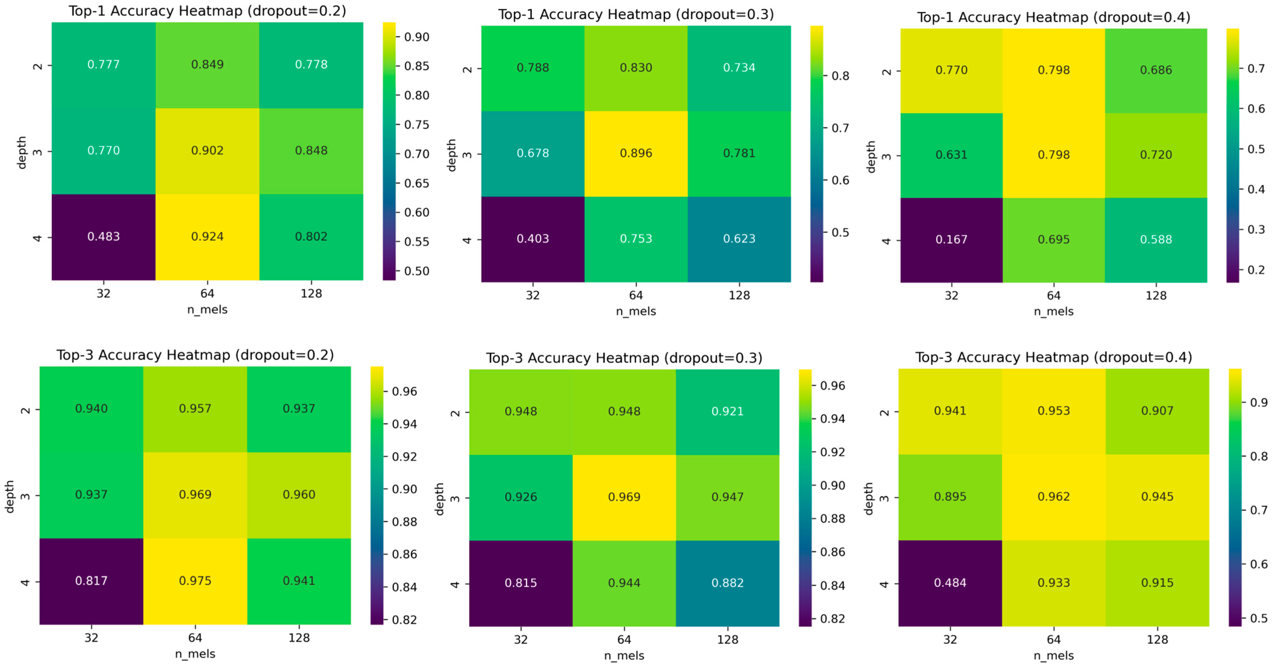
We have used ablation procedure for obtaining three main parameters of the system: number of Mel filterbanks (n_mels), number of CNN levels (depth), and dropout. The values used for n_mels are [32, 64, 128], for depth are [2, 3, 4], and for dropout are [0.2, 0.3, 0.4]. Ablation was run with 10 epochs for each combination of parameters. After the ablation procedure, we obtained the best parameters: n_mels = 64, depth = 4, and dropout = 0.2. These results are presented in Figure 3 as top-1 and top-3 accuracy heatmaps.

5.1. Audio Signal Processing

The audio signal processing module uses the torchaudio library to prepare raw audio data for the speech command recognition model. It performs several key steps:

• Loading and preprocessing audio:

• Audio files in wav format are loaded and converted to mono.
• Signals are resampled to 16 kHz, a standard choice for speech recognition tasks [6].
• Amplitude normalization is applied to ensure consistent volume levels across all samples.

2.

Mel spectrogram generation:

• The audio is divided into overlapping windows of n_fft = 1024 samples, with a hop length of 256 samples.
• Each window is transformed using Short-Time Fourier Transform (STFT) to obtain the frequency spectrum.
• The minimum frequency is 20 Hz, and maximum frequency is 8 kHz.
• The spectrum is projected onto 64 triangular filter banks according to the Mel scale, providing finer resolution at low frequencies and coarser resolution at high frequencies.
• The spectrogram is converted to decibel (dB) scale to enhance contrast and emphasize speech-relevant features.

3.

Padding and fixed-size input:

• Spectrograms are padded to 64 time steps. Clips longer than this are truncated. This ensures a consistent input shape for the CNN.

Each audio clip is represented as a 64 × 64 Mel spectrogram (frequency bins × time steps), capturing the most informative low- and mid-frequency content. These spectrograms are used as input to the CNN. Figure 4 illustrates the flow of the audio signal processing module, showing all steps from raw audio to model-ready features.

5.2. Convolutional Neural Network

The convolutional neural network (CNN) module is implemented using PyTorch and is designed to process Mel spectrograms as input. The network consists of three convolutional layers followed by a fully connected classifier head (ANN). The architecture is as follows:

• Convolutional layers:

• First layer: 16 output channels, 3 × 3 kernel, padding = 1, stride = 1, ReLU activation, 2 × 2 max pooling, 20% dropout.
• Second layer: 32 output channels, same kernel and stride, ReLU, 2 × 2 max pooling, 20% dropout.
• Third layer: 64 output channels, same kernel and stride, ReLU, 2 × 2 max pooling, 20% dropout.
• Fourth layer: 128 output channels, same kernel and stride, ReLU, 2 × 2 max pooling, 20% dropout.
• These convolutional layers learn local patterns in the Mel spectrogram, such as edges, harmonics, and transitions. Batch normalization is applied after each convolution to stabilize training and accelerate convergence. Max pooling reduces the spatial resolution, and dropout regularization helps prevent overfitting.

2.

Fully connected classifier (ANN head):

• The output of the final convolutional layer is flattened into a 1D vector.
• A hidden layer with 128 neurons applies ReLU activation and 20% dropout.
• The output layer maps these features to the number of classes (10 main commands, plus additional “silence” and “unknown” classes). A softmax activation produces probabilities for each class.

3.

Dataset handling and augmentation:

• The dataset includes ten main commands, along with “silence” and “unknown” classes. Silence samples are generated from background noise segments and recorded environmental sound from microphone, while unknown samples include words outside the main command set.
• A speaker-independent split ensures that training and validation sets do not share speakers, preventing overfitting and providing a realistic measure of generalization.
• For training, 70% of the dataset is used, for testing 15% and for validation 15%.
• During training, simple augmentations are applied to improve robustness: small random time shifts, additive background noise, and minor amplitude scaling.
• Random seeds are fixed to ensure reproducibility of the splits and augmentations. The random seed was 42 (for random, numpy, and torch libraries), and batch size was 16.
• Early stopping criterion was set to 10 epochs with no improvement in accuracy, after which the training stops.

4.

Training setup:

• The network is trained with cross-entropy loss and the Adam optimizer with learning rate of 0.001.
• Batch size, number of epochs, learning rate, and random seeds are fixed to ensure reproducibility. The number of epochs was 50.

5.

Operation and evaluation:

• The CNN extracts relevant features from the spectrogram, and the classifier head uses these features to assign probabilities to each class.
• Model performance is evaluated using top-1 and top-3 accuracy, per-class precision, recall, and F1 scores, including macro and micro averages.
• A speaker-independent split ensures that audio from the same speaker does not appear in both training and validation sets.

In summary, the CNN identifies local patterns in the audio spectrograms, while the classifier head interprets these patterns to make the final class decision. Figure 5 illustrates the complete CNN + classifier pipeline. This modular approach ensures that feature extraction and classification are clearly separated, making the model easier to analyze and optimize.

6. Results and Discussion

6.1. Computer Model Results

To assess the performance of the speech command recognition system, a speaker-independent evaluation protocol is applied. This ensures that no audio from a given speaker appears in both training and validation/test sets, preventing data leakage and overfitting. The CPU that was used is Intel i5 13450HX (Intel, Santa Clara, CA, USA) with 16GB of RAM and NVIDIA RTX 4060 Mobile GPU (NVIDIA, Santa Clara, CA, USA).

The model is evaluated using multiple complementary metrics:

• Top-1 and Top-3 accuracy:

  ○

  Top-1 accuracy measures the percentage of test samples for which the highest probability class matches the true label.

  ○

  Top-3 accuracy measures the percentage of samples for which the true label is among the three highest probability predictions.

• Per-class precision, recall, and F1-score:

  ○

  Precision: proportion of correct predictions among all predictions for a class.

  ○

  Recall: proportion of correctly predicted samples of a class among all true samples.

  ○

  F1-score: harmonic mean of precision and recall.

• Macro and micro-averages:

  ○

  Macro-average treats all classes equally, while micro-average accounts for class imbalance.

• A confusion matrix is computed to visualize classification performance across all classes.
• For binary or one-vs-all tasks, Receiver Operating Characteristic (ROC) curves are computed, and the Area Under the Curve (AUC) quantifies the discriminative ability of the model.

After training the model through 50 epochs, the training accuracy obtained was 96.05%, and the validation accuracy was 94.91%. The precision, recall, and F1-score of the individual classes are given in

Table 2. Precision, recall, and F1-score of individual classes.

Class	Precision	Recall	F1-Score
Down	0.95	0.93	0.94
Go	0.93	0.93	0.93
Left	0.98	0.96	0.97
No	0.92	0.96	0.94
Off	0.94	0.92	0.93
On	0.96	0.93	0.95
Right	0.97	0.96	0.97
Silence	0.98	1	0.99
Stop	0.98	0.99	0.98
Unknown	0.90	0.87	0.88
Up	0.89	0.95	0.92
Yes	0.98	0.98	0.98
Macro avg	0.95	0.95	0.95
Weighted avg	0.95	0.95	0.95
Micro	0.9479	0.9479	0.9479
Macro	0.9482	0.9479	0.9479

, along with macro and weighted average, and micro and macro-values. The Top-1 accuracy was 94.79%, and Top-3 accuracy was 98.84%. The ROC AUC value was 99.83%.

Table 2 summarizes the precision, recall, and F1-scores for each of the twelve classes. Most classes achieve consistently high values above 0.93, indicating balanced precision and recall. The “silence” and “stop” classes stand out with near-perfect performance (F1 = 0.99 and 0.98, respectively), while “unknown” and “up” are relatively more challenging, with F1-scores of 0.88 and 0.92. This suggests that the model occasionally confuses “unknown” inputs with standard commands and has some difficulty in distinguishing “up” under certain conditions.

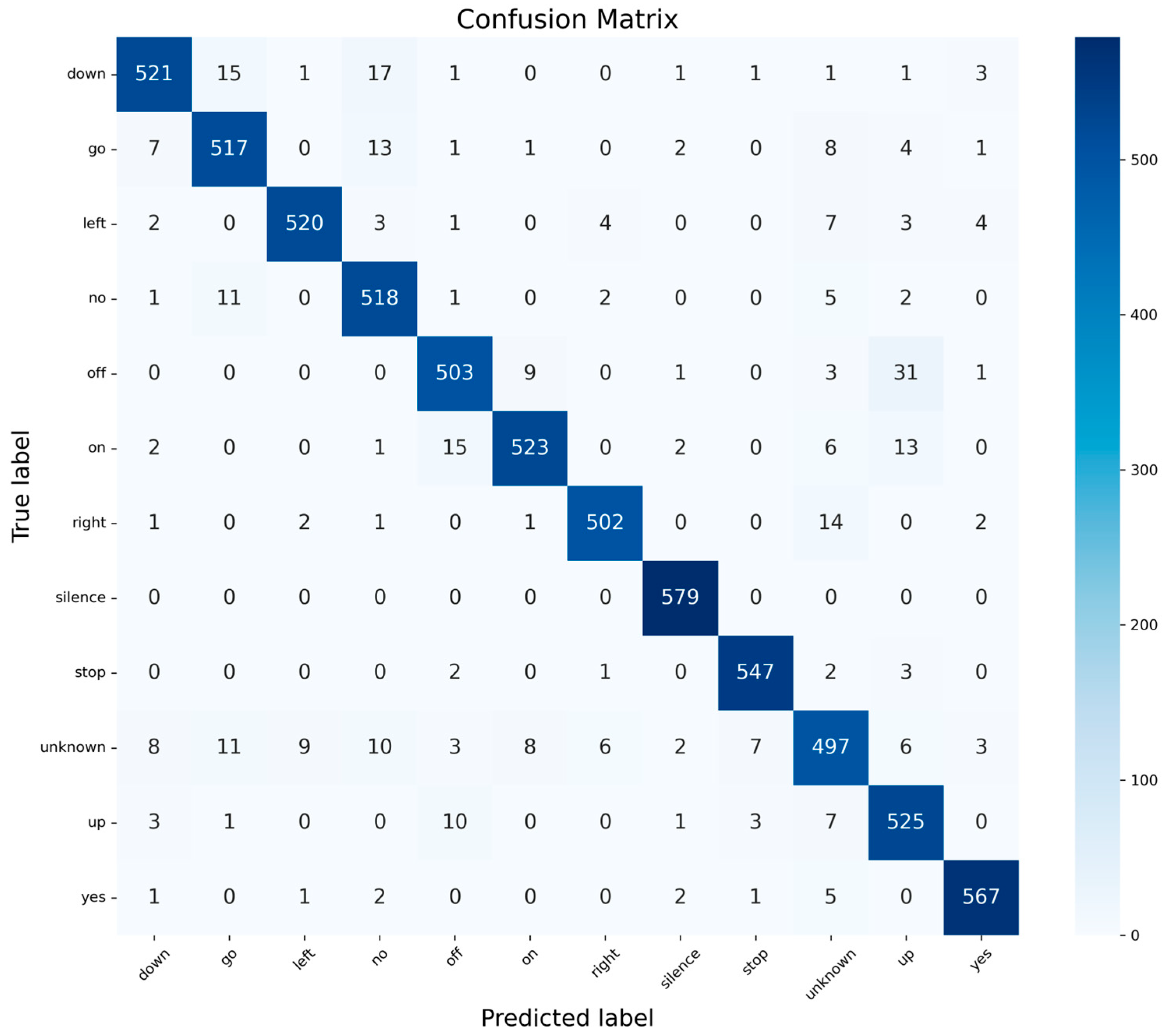
The aggregated results (macro, weighted, and micro averages) are highly consistent, all around 0.95, which indicates that the model performs uniformly across classes without being dominated by class imbalance. These findings align with the confusion matrix and ROC curve analysis, confirming the robustness of the classifier. The confusion matrix is given in Figure 6.

The confusion matrix shows that the model achieves consistently high accuracy across all classes, with the diagonal cells strongly dominating. Most speech commands such as “down” (521/561), “go” (517/546), “left” (520/541), “no” (518/540), “stop” (547/553), “up” (525/550), and “yes” (567/577) are recognized with very few misclassifications. The “silence” class is almost perfectly identified (579/579), confirming the effectiveness of the silence generation strategy.

Some mild confusion appears between semantically or acoustically similar words. For example, “off” has occasional misclassifications into “unknown” (31 instances), while “on” is sometimes predicted as “unknown” (13 cases). Similarly, “right” shows a small number of misclassifications into “unknown” and other directions. The “unknown” category itself is the most challenging, with scattered misclassifications across multiple command labels, reflecting its broad and heterogeneous nature.

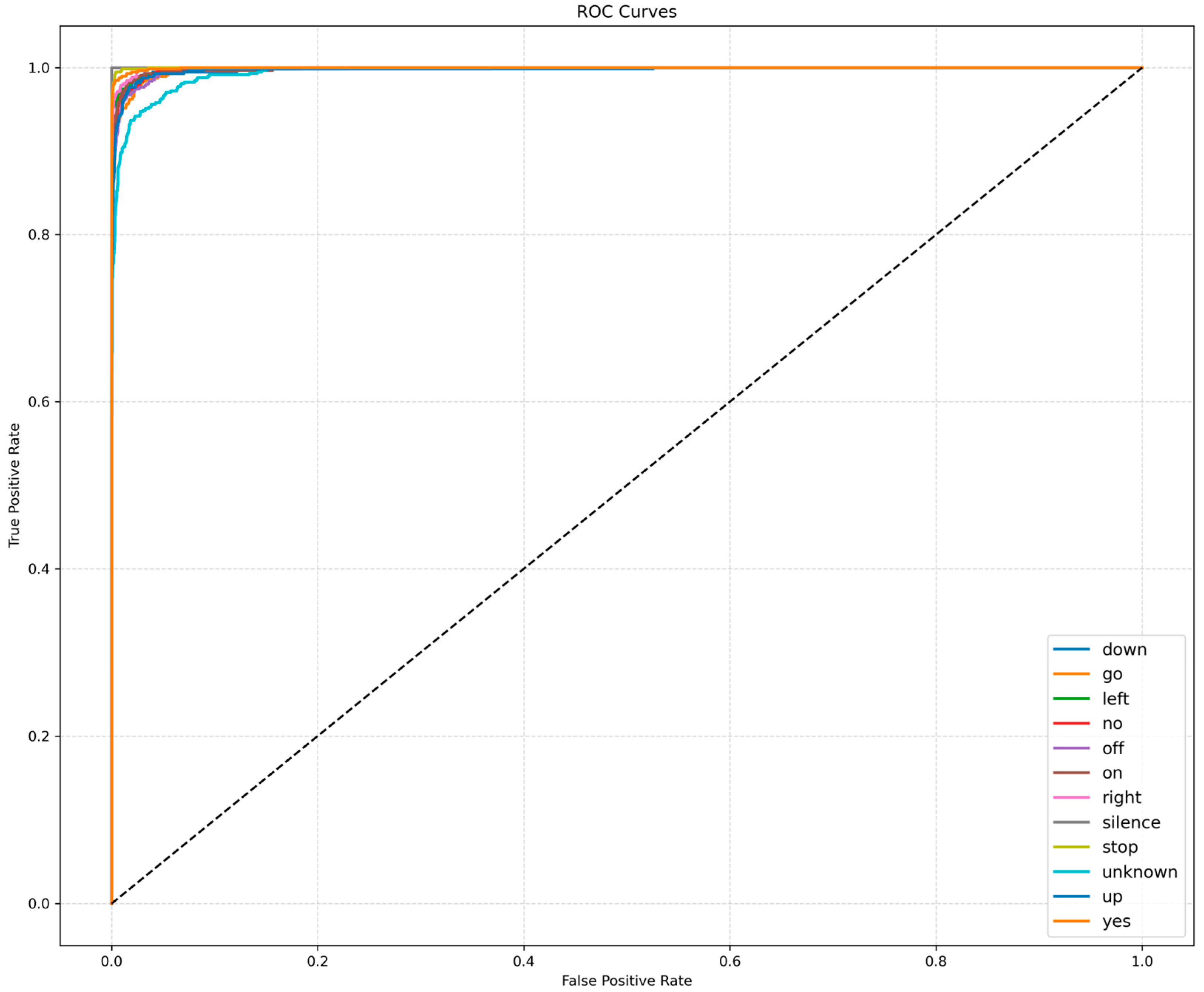
The ROC curves of individual classes are given in Figure 7. The ROC curves demonstrate excellent discriminative performance across all twelve classes. Most curves are tightly clustered in the upper-left corner of the plot, indicating very high true positive rates and extremely low false positive rates. This is further confirmed by the near-vertical rise in the curves and their proximity to the top edge of the plot, suggesting that the corresponding Area Under the Curve (AUC) values are close to 1.0.

6.2. Fog Computer Results

As a Fog computer, the Raspberry Pi 5 (Raspberry Pi Foundation, Cambridge, UK) with 8GB of RAM was used. The model trained on the computer was saved in “pth” format for use on Raspberry Pi. The same data that were used for testing on the computer were used on Raspberry Pi. Apart from the model, the Fog device also incorporates audio processing module.

The results obtained from running the model on the Raspberry Pi are identical to those achieved on the computer version of the application. This demonstrates that the deployment on embedded hardware does not compromise the predictive performance of the model. The consistency across platforms indicates that the trained model is both optimal and well balanced, maintaining high accuracy and stable generalization even under the resource constraints of a Fog computing device. These findings further validate the suitability of the proposed system for real-world, low-power, and edge-based speech recognition applications.

To assess the computational efficiency and deployment feasibility of the CNN model on embedded devices, we conducted a systematic evaluation of three model variants: the original FP32 model, a pruned FP32 model, and a dynamically quantized INT8 model. For each variant, we measured the total number of parameters, sparsity, model file size, single-shot inference latency, throughput, memory footprint, and CPU utilization using a representative Mel spectrogram input. Pruning was applied to convolutional and linear layers, removing 50% of weights to reduce sparsity, while dynamic INT8 quantization further reduced weight precision for improved memory efficiency. Latency and throughput were computed over multiple forward passes, and memory and CPU usage were monitored via the Python version 3.12 psutil library. This evaluation provides quantitative insight into the trade-offs between model size, computational complexity, and real-time inference performance, serving as a basis for deployment on resource-constrained platforms such as the Raspberry Pi 5. These results are presented in

Table 3. Main parameters of the various Raspberry Pi CNN models.

Parameter	Main Model	Pruned Model	Quantized Model
Parameter count	295,916	295,916	97,632
Nonzero parameters	295,916	148,388	49,176
Sparsity	0%	49.85%	49.63%
Model size	1.15 MB	1.15 MB	0.58 MB
FLOPS	14.38 MFLOPs	14.38 MFLOPs	14.18 MFLOPs
Single inference latency	3.04 ms	3.47 ms	5.8 ms
Throughput	329.28 samples/s	288.50 samples/s	172.53 samples/s
Memory footprint	418.94 MB	425.23 MB	429.89 MB
CPU utilization	6.8%	7%	7.2%

.

The original FP32 model has 296,916 parameters and runs very fast, with low latency and high throughput. After pruning roughly 50% of the weights, the model size stays the same, but the number of active parameters is halved. Surprisingly, latency increased slightly and throughput dropped, likely because standard CPUs do not benefit much from sparse weights. Finally, after INT8 quantization, the model size is cut in half, but latency increases and throughput drops further, as integer operations are less parallelized on the CPU, though memory footprint remains similar.

The application for speech command recognition was also developed on Raspberry Pi. Exemplary results are presented in Figure 8.

The Raspberry Pi application includes:

• Buttons “Start Recording” and “Stop Recording” for starting and stopping the voice recording via microphone and “Play Last” for playing the last recorded command.
• Mel spectrogram of the recorded command.
• Top three predictions with probabilities.

We have also connected a microphone to Raspberry Pi to test the model. The microphone is Fifine A2 with advanced echo and noise cancellation [44]. Each command was spoken out ten times, and the results were obtained. There were three participants, two males and one female, testing the commands in quiet and noisy conditions (music in the background). The results of the prediction are probabilities of top three recognized commands. These probabilities are the result of the softmax Torch method that is applied to the CNN model. The average probabilities for each command are given in

Table 4. Average probabilities for each command, P1—male participant, P2—male participant, P3—female participant.

Command	P1 Quiet	P2 Quiet	P3 Quiet	P1 Noisy	P2 Noisy	P3 Noisy	Average Quiet	Average Noisy	Average Overall
Down	0.96	0.98	0.94	0.97	0.99	0.78	0.96	0.91	0.94
Go	0.99	0.95	0.85	0.99	0.95	0.94	0.93	0.96	0.95
Left	1	0.98	0.92	1	1	0.91	0.97	0.97	0.97
No	0.98	0.97	0.93	0.99	0.96	0.89	0.96	0.95	0.95
Off	1	0.96	0.96	1	0.99	0.89	0.97	0.96	0.97
On	0.99	1	0.99	0.99	1	0.97	0.99	0.99	0.99
Right	1	0.98	0.93	0.98	0.99	0.98	0.97	0.98	0.98
Stop	0.98	0.91	0.89	0.93	0.68	0.59	0.93	0.73	0.83
Up	1	0.99	0.99	0.99	1	0.99	0.99	0.99	0.99
Yes	1	1	1	0.99	1	0.99	1.00	0.99	1.00

. It should be noted that all participants used Serbian as their mother tongue.

Table 4 shows the recognition accuracy of 10 voice commands across three participants (P1–P3) in quiet and noisy environments. Overall, the model performs very well, with most commands reaching above 95% accuracy.

• Quiet environment: Most commands are recognized almost perfectly, with averages around 96–100%. “Stop” is slightly lower (93%).
• Noisy environment: Accuracy drops for some commands, particularly “down” (91%) and “stop” (73%), indicating these are more sensitive to background noise. Commands like “on”, “up”, and “yes” remain highly robust (≥99%).
• Overall averages: Across all commands and participants, the model achieves about 95–98% accuracy, showing strong performance even under noise, but “stop” is the most challenging command in noisy conditions.

The “silence” class was tested by having a silent or noisy background (music playing) in 20 cases, and in all cases the “silence” class was classified. For the “unknown” class, the participants spoke Serbian words for numbers 1 to 10, and in 80% of cases the recognized class was “unknown”. In two cases, the word “dva” (“two”) was labeled as “on”, and “sedam” (“seven”) was labeled as “down”.

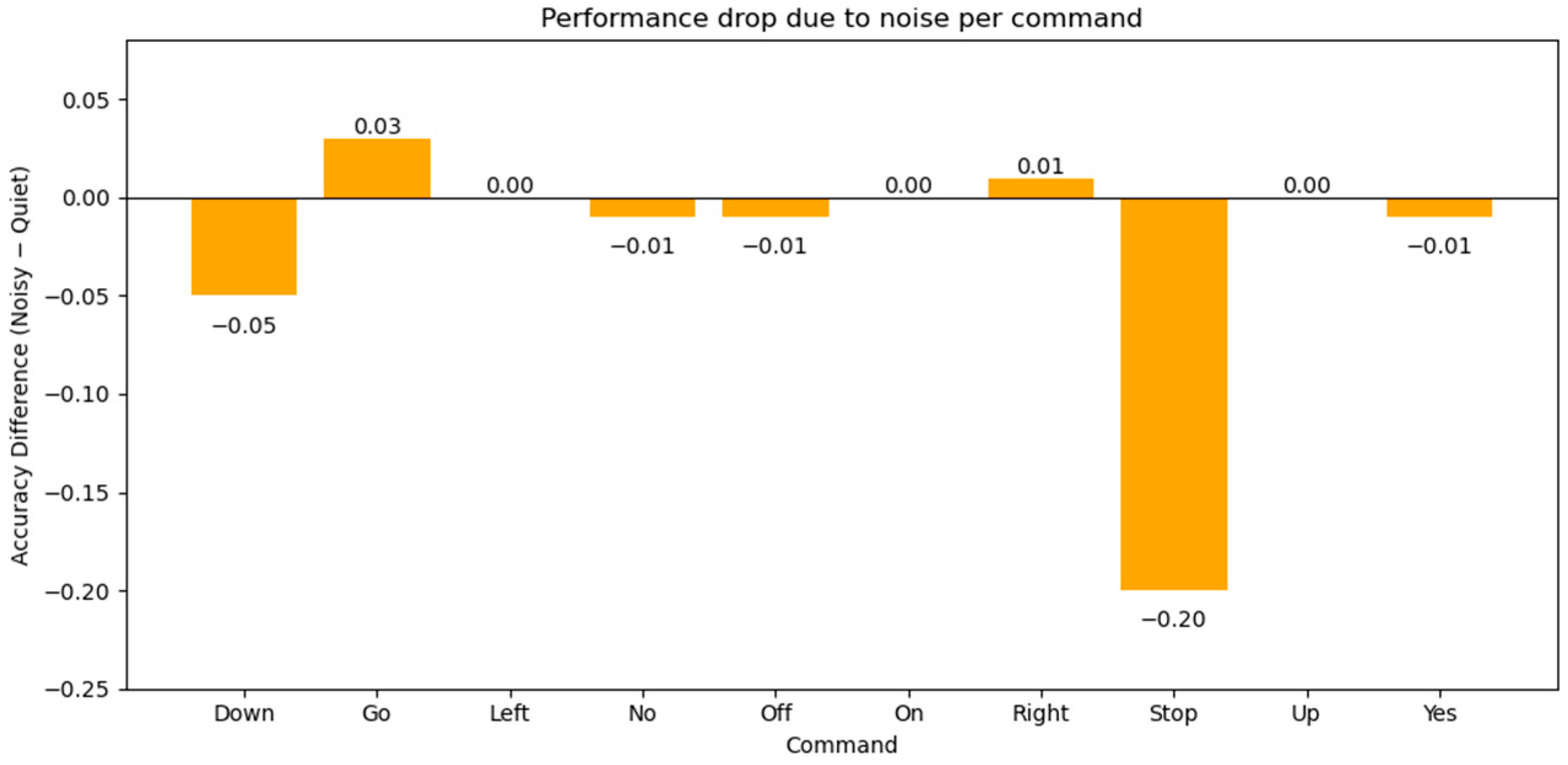
Figure 9 represents performance drops due to noise, per command. As can be seen, the greatest drop is for “stop” command, and we have a slight increase in performance for “go” and “right” command, while “left”, “on”, and “up” remained the same.

6.3. Comparison with Relevant Models

According to the experiments carried out in this study, together with an analysis of previously reported results, we conducted a comparison of our model against representative baselines such as YAMNet, EdgeSpeechNets, and TinySpeech. YAMNet has demonstrated strong performance, achieving an accuracy of 92.7% on the ESC-50 dataset [10]. However, its relatively large parameter number of around 6.5 million and inference latency of approximately 100 ms limit its applicability for real-time deployment on embedded platforms [10]. EdgeSpeechNet was explicitly designed for small-footprint keyword spotting and provides a strong baseline: the best performing variant, EdgeSpeechNet-A, reaches about 97% accuracy on the Google Speech Commands dataset, while requiring only around 0.3 million parameters and achieving a latency close to 10 ms with roughly 0.1 GFLOPs of computation [9]. TinySpeech-X, one of the proposed TinySpeech models [8], achieves an accuracy of 94.6% on the Google Speech Commands dataset while maintaining an extremely small parameter count of approximately 10.8 thousand and requiring about 10.9 million multiply-add operations. These results demonstrate that TinySpeech provides a favorable trade-off between accuracy and computational efficiency

Compared to these baselines, our proposed model achieves competitive accuracy while maintaining a significantly lower computational footprint. This positions it as a favorable solution for embedded and low-power scenarios, offering a balanced trade-off between performance and efficiency. This could also be the single most valuable contribution of our work.

7. Conclusions

In this paper, we proposed a deep learning system for speech command recognition that can be deployed to Fog devices such as Raspberry Pi. The system comprises audio processing module with deep learning subsystem, composed of four-layer convolutional neural network and linear artificial neural network head. The final accuracy of 96.05% was obtained.

We have also implemented a Raspberry Pi application that uses a saved deep learning model to categorize spoken commands with a microphone. All commands had very good results. In order to improve the system further, it would be of great significance to record several hundred commands to train the model on them. In this way, the accuracy of the Raspberry Pi application would be significantly better.

While the proposed speech command recognition system demonstrates high accuracy on the selected dataset, several limitations must be acknowledged. First, the model is trained on a limited set of ten commands plus “silence” and “unknown”, which restricts its generalizability to a broader vocabulary. Second, variations in speaker accents and voice characteristics may degrade performance, as the dataset does not fully cover global linguistic diversity. Third, the system has primarily been evaluated under close-range recording conditions; far-field scenarios and environmental noise may reduce recognition accuracy. Finally, out-of-distribution words or phrases are likely to be misclassified, highlighting the need for additional strategies for unknown or rare inputs. Future work should address these limitations by expanding the command set, including more diverse speakers, and testing robustness under challenging acoustic conditions.

References

1. Warden, P. Speech Commands: A Public Dataset for Single-Word Speech Recognition. 2017. Available online: http://download.tensorflow.org/data/speech_commands_v0.01.tar.gz (accessed on 10 September 2025).
2. Chen, J.; Teo, T.H.; Kok, C.L.; Koh, Y.Y. A Novel Single-Word Speech Recognition on Embedded Systems Using a Convolution Neuron Network with Improved Out-of-Distribution Detection. Electronics 2024, 13, 530. [Google Scholar] [CrossRef]
3. Zinemanas, P.; Rocamora, M.; Miron, M.; Font, F.; Serra, X. An Interpretable Deep Learning Model for Automatic Sound Classification. Electronics 2021, 10, 850. [Google Scholar] [CrossRef]
4. Sainath, T.N.; Parada, C. Convolutional neural networks for small-footprint keyword spotting. In Proceedings of the Interspeech, Dresden, Germany, 6–10 September 2015; pp. 1478–1482. [Google Scholar] [CrossRef]
5. Zhang, Y.; Suda, N.; Lai, L. Hello Edge: Keyword Spotting on Microcontrollers. arXiv 2017, arXiv:1711.07128. [Google Scholar] [CrossRef]
6. Warden, P. Speech Commands: A dataset for Limited-Vocabulary Speech Recognition. arXiv 2018, arXiv:1804.03209. [Google Scholar] [CrossRef]
7. De Andrade, D.C.; Leo, S.; Viana, M.L.D.S.; Bernkopf, C. A neural attention model for speech command recognition. arXiv 2018, arXiv:1808.08929. [Google Scholar] [CrossRef]
8. Wong, A.; Famouri, M.; Pavlova, M.; Surana, S. Tinyspeech: Attention condensers for deep speech recognition neural networks on edge devices. arXiv 2020, arXiv:2008.04245. [Google Scholar] [CrossRef]
9. Lin, Z.Q.; Chung, A.G.; Wong, A. Edgespeechnets: Highly efficient deep neural networks for speech recognition on the edge. arXiv 2018, arXiv:1810.08559. [Google Scholar] [CrossRef]
10. Kuzminykh, I.; Shevchuk, D.; Shiaeles, S.; Ghita, B. Audio Interval Retrieval Using Convolutional Neural Networks. In Internet of Things, Smart Spaces, and Next Generation Networks and Systems; Galinina, O., Andreev, S., Balandin, S., Koucheryavy, Y., Eds.; NEW2AN 2020, ruSMART 2020; Lecture Notes in Computer Science; Springer: Cham, Switzerland, 2020; Volume 12525. [Google Scholar] [CrossRef]
11. Schmid, F.; Koutini, K.; Widmer, G. Dynamic Convolutional Neural Networks as Efficient Pre-Trained Audio Models. IEEE/ACM Trans. Audio Speech Lang. Process. 2024, 32, 2227–2241. [Google Scholar] [CrossRef]
12. Baevski, A.; Zhou, H.; Mohamed, A.; Auli, M. wav2vec 2.0: A Framework for Self-Supervised Learning of Speech Representations. arXiv 2020, arXiv:2006.11477. [Google Scholar] [CrossRef]
13. Chang, H.-J.; Bhati, S.; Glass, J.; Liu, A.H. USAD: Universal Speech and Audio Representation via Distillation. arXiv 2025, arXiv:2506.18843. [Google Scholar] [CrossRef]
14. Shor, J.; Jansen, A.; Maor, R.; Lang, O.; Tuval, O.; Quitry, F.d.C.; Tagliasacchi, M.; Shavitt, I.; Emanuel, D.; Haviv, Y. Towards Learning a Universal Non-Semantic Representation of Speech. In Proceedings of the Interspeech, Shanghai, China, 25–29 October 2020; pp. 140–144. [Google Scholar] [CrossRef]
15. Gulati, A.; Qin, J.; Chiu, C.-C.; Parmar, N.; Zhang, Y.; Yu, J.; Han, W.; Wang, S.; Zhang, Z.; Wu, Y.; et al. Conformer: Convolution-augmented Transformer for Speech Recognition. In Proceedings of the Interspeech, Shanghai, China, 25–29 October 2020; pp. 5036–5040. [Google Scholar] [CrossRef]
16. Han, W.; Zhang, Z.; Zhang, Y.; Yu, J.; Chiu, C.-C.; Qin, J.; Gulati, A.; Pang, R.; Wu, Y. ContextNet: Improving Convolutional Neural Networks for Automatic Speech Recognition with Global Context. In Proceedings of the Interspeech, Shanghai, China, 25–29 October 2020; pp. 3610–3614. [Google Scholar] [CrossRef]
17. Bartoli, P.; Bondini, T.; Veronesi, C.; Giudici, A.; Antonello, N.; Zappa, F. End-to-End Efficiency in Keyword Spotting: A System-Level Approach for Embedded Microcontrollers. arXiv 2025, arXiv:2509.07051. [Google Scholar] [CrossRef]
18. Alhashimi, S.A.; Aliedani, A. Embedded Device Keyword Spotting Model with Quantized Convolutional Neural Network. Int. J. Eng. Trends Technol. 2025, 73, 117–123. [Google Scholar] [CrossRef]
19. Kadhim, I.J.; Abdulabbas, T.E.; Ali, R.; Hassoon, A.F.; Premaratne, P. Enhanced speech command recognition using convolutional neural networks. J. Eng. Sustain. Dev. 2024, 28, 754–761. [Google Scholar] [CrossRef]
20. Pervaiz, A.; Hussain, F.; Israr, H.; Tahir, M.A.; Raja, F.R.; Baloch, N.K.; Ishmanov, F.; Zikria, Y.B. Incorporating Noise Robustness in Speech Command Recognition by Noise Augmentation of Training Data. Sensors 2020, 20, 2326. [Google Scholar] [CrossRef] [PubMed]
21. Chen, C.; Hou, N.; Hu, Y.; Shirol, S.; Chng, E.S. Noise-robust speech recognition with 10 minutes unparalleled in-domain data. In Proceedings of the IEEE International Conference on Acoustics, Speech and Signal Processing (ICASSP), Singapore, 22–27 May 2022; pp. 7717–7721. [Google Scholar] [CrossRef]
22. Porjazovski, D.; Moisio, A.; Kurimo, M. Out-of-distribution generalisation in spoken language understanding. In Proceedings of the Interspeech Kos, Greece, 1–5 September 2024; pp. 807–811. [Google Scholar] [CrossRef]
23. Baranger, A.; Maison, L. Evaluating and Improving the Robustness of Speech Command Recognition Models to Noise and Distribution Shifts. arXiv 2025, arXiv:2507.23128. [Google Scholar] [CrossRef]
24. Chernyak, B.R.; Segal, Y.; Shrem, Y.; Keshet, J. PatchDSU: Uncertainty Modeling for Out of Distribution Generalization in Keyword Spotting. arXiv 2025, arXiv:2508.03190. [Google Scholar] [CrossRef]
25. Rabiner, L.; Juang, B.H. Fundamentals of Speech Recognition; Prentice Hall: Englewood Cliffs, NJ, USA, 1993. [Google Scholar]
26. Jurafsky, D.; Martin, J.H. Speech and Language Processing, 3rd ed. Available online: https://web.stanford.edu/~jurafsky/slp3/ (accessed on 10 September 2025).
27. Zhou, Q.; Shan, J.; Ding, W.; Wang, C.; Yuan, S.; Sun, F.; Li, H.; Fang, B. Cough recognition based on Mel-spectrogram and convolutional neural network. Front. Robot. AI 2021, 8, 580080. [Google Scholar] [CrossRef]
28. Sharan, R.V.; Berkovsky, S.; Liu, S. Voice Command Recognition Using Biologically Inspired Time-Frequency Representation and Convolutional Neural Networks. In Proceedings of the 2020 42nd Annual International Conference of the IEEE Engineering in Medicine & Biology Society (EMBC), Montreal, QC, Canada, 20–24 July 2020; pp. 998–1001. [Google Scholar] [CrossRef]
29. Stevens, S.S.; Volkmann, J.; Newman, E.B. A scale for the measurement of the psychological magnitude pitch. J. Acoust. Soc. Am. 1937, 8, 185–190. [Google Scholar] [CrossRef]
30. Davis, S.B.; Mermelstein, P. Comparison of parametric representations for monosyllabic word recognition in continuously spoken sentences. IEEE Trans. Acoust. Speech Signal Process. 1980, 28, 357–366. [Google Scholar] [CrossRef]
31. Gemmeke, J.F.; Ellis, D.P.W.; Freedman, D.; Jansen, A.; Lawrence, W.; Moore, R.C.; Plakal, M.; Ritter, M. AudioSet: An ontology and human-labeled dataset for audio events. In Proceedings of the IEEE International Conference on Acoustics, Speech and Signal Processing (ICASSP), New Orleans, LA, USA, 5–9 March 2017; pp. 776–780. [Google Scholar] [CrossRef]
32. O’Shaughnessy, D. Speech Communication: Human and Machine; Addison-Wesley: Boston, MA, USA, 1987. [Google Scholar]
33. Feichtinger, H.G.; Luef, F. Gabor Analysis and Algorithms; Engquist, B., Ed.; Encyclopedia of Applied and Computational Mathematics; Springer: Berlin/Heidelberg, Germany, 2015. [Google Scholar] [CrossRef]
34. Mallat, S. A Wavelet Tour of Signal Processing; Academic Press: Cambridge, MA, USA, 1999. [Google Scholar]
35. Li, Z.; Liu, F.; Yang, W.; Peng, S.; Zhou, J. A Survey of Convolutional Neural Networks: Analysis, Applications, and Prospects. IEEE Trans. Neural Netw. Learn. Syst. 2021, 33, 6999–7019. [Google Scholar] [CrossRef] [PubMed]
36. Krizhevsky, A.; Sutskever, I.; Hinton, G. ImageNet Classification with Deep Convolutional Neural Networks. Adv. Neural Inf. Process. Syst. 2012, 25, 1–9. [Google Scholar] [CrossRef]
37. Gu, J.; Wang, Z.; Kuen, J.; Ma, L.; Shahroudy, A.; Shuai, B.; Liu, T.; Wang, X.; Wang, G.; Cai, J.; et al. Recent advances in convolutional neural networks. Pattern Recognit. 2018, 77, 354–377. [Google Scholar] [CrossRef]
38. Krichen, M. Convolutional Neural Networks: A Survey. Computers 2023, 12, 151. [Google Scholar] [CrossRef]
39. O’shea, K.; Nash, R. An Introduction to Convolutional Neural Networks. arXiv 2015, arXiv:1511.08458. [Google Scholar] [CrossRef]
40. Kingma, D.P.; Ba, J. Adam: A method for stochastic optimization. arXiv 2014, arXiv:1412.6980. [Google Scholar] [CrossRef]
41. Cantiabela, Z.; Pardede, H.F.; Zilvan, V.; Sulandari, W.; Yuwana, R.S.; Supianto, A.A.; Krisnandi, D. Deep learning for robust speech command recognition using convolutional neural networks (CNN). In Proceedings of the 2022 International Conference on Computer, Control, Informatics and Its Applications, Virtually, 22–23 November 2022; pp. 101–105. [Google Scholar] [CrossRef]
42. Li, X.; Zhou, Z. Speech command recognition with convolutional neural network. CS229 Stanf. Educ. 2017, 31, 1–6. [Google Scholar]
43. Srivastava, N.; Hinton, G.; Krizhevsky, A.; Sutskever, I.; Salakhutdinov, R. Dropout: A simple way to prevent neural networks from overfitting. J. Mach. Learn. Res. 2014, 15, 1929–1958. [Google Scholar]
44. Fifine Ampligame A2 Microphone. Available online: https://fifinemicrophone.com/products/fifine-ampligame-a2 (accessed on 10 September 2025).
Figure 1. Procedure for implementing CNN; * stands for convolution operation.
Electronics 14 03793 g001
Figure 2. Main modules of speech recognition system.
Electronics 14 03793 g002
Figure 3. Top-1 and top-3 accuracy heatmaps for different values of ablation parameters.
Electronics 14 03793 g003
Figure 4. Flowchart of audio signal processing module.
Electronics 14 03793 g004
Figure 5. Flow diagram of CNN module.
Electronics 14 03793 g005
Figure 6. Confusion matrix of the model.
Electronics 14 03793 g006
Figure 7. ROC curves of the individual classes.
Electronics 14 03793 g007
Figure 8. Illustration of the Raspberry Pi application.
Electronics 14 03793 g008
Figure 9. Performance drops due to noise, per command.
Electronics 14 03793 g009