Article

Bayesian–Geometric Fusion: A Probabilistic Framework for Robust Line Feature Matching

1
School of Civil Engineering and Architecture, Changzhou Institute of Technology, Changzhou 213032, China
2
School of Computing and Data Science, The University of Hong Kong, Hong Kong 999077, China
3
School of Computer Science and Engineering, Nanjing University of Science and Technology, Nanjing 210014, China
*
Authors to whom correspondence should be addressed.
Electronics 2025, 14(19), 3783; https://doi.org/10.3390/electronics14193783
Submission received: 13 August 2025 / Revised: 21 September 2025 / Accepted: 22 September 2025 / Published: 24 September 2025
(This article belongs to the Section Circuit and Signal Processing)

Abstract

Line feature matching is a fundamental and extensively studied subject in the fields of photogrammetry and computer vision. Traditional methods, which rely on handcrafted descriptors and distance-based filtering outliers, frequently encounter challenges related to robustness and a high incidence of outliers. While some approaches leverage point features to assist line feature matching by establishing the invariant geometric constraints between points and lines, this typically results in a considerable computational load. In order to overcome these limitations, we introduce a novel Bayesian posterior probability framework for line matching that incorporates three geometric constraints: the distance between line feature endpoints, midpoint distance, and angular consistency. Our approach initially characterizes inter-image geometric relationships using Fourier representation. Subsequently, we formulate the posterior probability distributions for the distance constraint and the uniform distribution based on the constraint of angular consistency. By calculating the joint probability distribution under three geometric constraints, robust line feature matches are iteratively optimized through the Expectation–Maximization (EM) algorithm. Comprehensive experiments confirm the effectiveness of our approach: (i) it outperforms state-of-the-art (including deep learning-based) algorithms in match count and accuracy across common scenarios; (ii) it exhibits superior robustness to rotation, illumination variation, and motion blur compared to descriptor-based methods; and (iii) it notably reduces computational overhead in comparison to algorithms that involve point-assisted line matching.

1. Introduction

Feature matching (refers to point and line) is a crucial task in image processing and analysis, playing a central role in image-based research fields such as computer vision, artificial intelligence, industrial vision inspection, and autonomous driving, etc. It has a broad range of practical applications, including pose estimation [1,2], SFM (structure from motion) [3,4], 3D measurement [5] and image manipulation localization [6], SLAM (simultaneous localization and mapping) [7,8], optical flow estimation [9], augmented reality [10], and image stitching or fusion [11,12,13]. In the community of photogrammetry and remote sensing, feature matching, especially line feature, has also garnered significant attention from researchers [14]. Tasks in these domains, such as high-precision 3D reconstruction and urban modeling, building and road extraction monitoring, and image registration, heavily rely on the accuracy and robustness of line feature matching [15]. In vision-processing work, point and line visual features are regarded as foundational visual elements, and their accurate and robust matching also relates to the success of specific functions and applications.
Point features, a fundamental and widely used visual element in digital imagery, have received significant attention in the community of image processing. Initially, the detection and matching of feature points have evolved from original methods based on locally defined corner features derived from image grayscale values (e.g., Harris, Sift, Surf, ORB, Fast, Kaze, etc.) to deep learning-based approaches (e.g., SuperPoint, D2-Net, Lift, LF-Net), achieving substantial progress [16,17,18]. Researchers have made significant strides in improving the efficiency and accuracy of point feature detection algorithms across various scenarios. Additionally, the matching strategy for point feature has also witnessed the development of several excellent algorithms, such as GMS proposed by Bian et al. [19] and SuperGlue proposed by Sarlin et al. [20]. These methods, which range from descriptor-based geometric and motion constraints to deep learning-driven descriptor matching, have found broad applications in areas such as everyday life, robotic navigation, and industrial automation.
In comparison to point features, line features offer enhanced structural information regarding environments and objects, facilitating a more precise description and depiction of environmental characteristics. This capability is particularly advantageous for scene perception and reconstruction, notably in the context of robots or other mobile platforms [21]. Although point feature extraction and matching have demonstrated considerable robustness and efficiency, challenges persist in the matching of line features, presenting opportunities for further enhancement [22]. The matching of feature pairs is crucial for various practical applications such as pose estimation, visual navigation, and image stitching, where the integration of both point and line features, or the utilization of line feature constraints, serves to improve precision and accuracy in specific scenarios [23,24]. Despite progress in line feature matching, the robust correspondence of line features remains a fundamental, unresolved issue in geometric computer vision and aerial photogrammetry.
The matching of line features is essential for practical applications, and the research on line feature matching has also begun to be involved relatively early; however, deficiencies persist in existing line-matching algorithms. Based on a thorough review of the current literature and comprehensive analysis on line feature matching [15], we have identified several shortcomings in current feature matching methodologies, as outlined below:
(i)
It would be rude to “hard filter” based on the distance metric between the binary descriptors of the line feature to obtain the line feature matching pair. This can result in the loss of potentially correct line feature matching pairs. It is also unfriendly for low-texture, illuminated image pairs, as well as image pairs with rotation components.
(ii)
Relying on jointly constructed point–line invariants imposes significant limitations. Firstly, the accuracy of matching decreases in regions lacking texture and sparse point features. Secondly, the resultant computational complexity prohibits real-time deployment in time-sensitive applications.
To address the challenges associated with line feature matching, we proposed a novel approach that utilizes the Fourier series to describe the transformation mapping relationship between matching pairs of images. Our method enhances the accuracy of line feature matching by constructing posterior probability models that incorporates geometric constraints, specifically focusing on endpoints and midpoint distances. In addition to these geometric constraints, we introduce angular constraints to better account for the orientation of line features. By establishing a uniform distribution model, we can accurately estimate the posterior probability of each potential matching pair. The process begins with an initial set of matching pairs. We employ an iterative search process to identify unmatched line features near the already matched lines, thereby increasing the number of potential matching pairs. At last, combining the line feature descriptors with the Fourier series representations, our proposed method iteratively searches the line feature matching pairs, and updates the parameters of posterior probability estimation, achieving more accurate and robust line feature matching.
This study addresses the challenges inherent in line feature matching by providing a comprehensive review and analysis of prominent line-matching algorithms, offering researchers a systematic and in-depth perspective on current methodologies. The key contributions of this work are summarized below:
  • We propose a novel line feature matching algorithm that directly utilizes feature descriptors, eliminating the need for mismatch filtering based on rough geometric constraint condition or the computationally intensive process of computing homography matrix. Importantly, our approach achieves complete line feature matching without requiring supplementary point feature correspondences.
  • This work introduces, to our knowledge, the first posterior probability distribution model specifically designed for line feature matching by exploiting intrinsic geometric properties. The proposed model synergistically combines spatial distance (endpoint and midpoint distances) and angular consistency through uniform distribution modeling, to optimize line feature correspondence determination in a unified probabilistic framework.
  • We conducted extensive evaluations across challenging visual scenarios including low-texture environments, significant viewpoint rotations, and variable lighting conditions. Quantitative and qualitative comparisons with state-of-the-art methods demonstrate our algorithm’s superior performance. Comprehensive ablation studies further validate the robustness and effectiveness of the proposed approach.
The paper is structured as follows: Section 2 provides a review of existing methods and their limitations in line feature matching. Section 3 outlines the methodology and key steps of our proposed algorithm. Section 4 presents a comprehensive comparative analysis of our method’s performance, supported by experiments on various image pairs. Section 5 discusses and summarizes the shortcomings and advantages of our method. The paper concludes in Section 6 with a summary of findings and recommendations for future research.

2. Related Works

Most existing line matching approaches typically involve four core stages: (1) detection and extraction of line features, (2) formulation and computation of distinctive descriptors, (3) initial line feature matching pairs, and (4) refinement of matched pairs through geometric consistency verification [25]. The line feature matching algorithms or strategies can generally be classified into three categories: single-line matching, group-based matching, and line matching based on deep learning.

2.1. Single Line Feature Matching

Line feature descriptors, which encode basic geometric characteristics or inter-segment relationships, represent the most intuitive solution for individual line segment matching [26]. Wang et al. [27] proposed the Mean Standard Deviation Line Descriptor (MLSD), a statistical descriptor derived from gradient distributions in four directions across sub-regions of a line’s support area, improving robustness in moderately textured images. Nonetheless, his method suffers from non-robustness and struggles with accuracy when faced with scale variations. Building upon this research, Zhang et al. [28] proposed a hybrid line-matching technique integrating local gradient patterns with global line structures, and the proposed approach is highly robust with multiple image distortions and can also handle scale variations to some degree. However, MSLD-based line matching is not optimal in indoor, texture-sparse scenes. To overcome this limitation, Zhang et al. [29] developed the line band descriptor (LBD), a novel approach that computes descriptors within line support regions by integrating both local appearance characteristics and geometric relationships, thereby enhancing matching performance in texture-deficient environments through geometric consistency verification.
Bay et al. [30] proposed an innovative line segment matching technique that integrates visual appearance and spatial configuration, surpassing conventional descriptor-based approaches. Their approach demonstrates robust performance in establishing accurate correspondences between line features across images captured from substantially distinct perspectives. Vogern et al. [31] further enhanced wide-baseline line matching by incorporating scale invariance into line descriptors, modifying Bay’s method and MSLD. Simultaneously, Li et al. [32] proposed the Line Junction Line (LJL) framework, establishing affine-invariant regions by linking line intersection points with intensity peaks. These regions subsequently employ SIFT [33] descriptors instead of traditional line descriptors for feature matching.
Under extreme illumination variations, Lin et al. [34] developed the illumination-invariant line binary (IILB) descriptor, which performs multi-scale band difference analysis in line support regions to achieve photometric invariance. This computationally efficient approach leverages integral image techniques, demonstrating particular advantages for resource-constrained systems. In a complementary approach, Wang et al. [35] tackled low-texture environments by combining edge detection and graph-based matching techniques. This fusion strategy resulted in robust performance in scenarios with few features.

2.2. Line Matching in Group

In cases where there is a substantial rotational disparity between image pairs, the efficacy of single-line-matching techniques reliant on descriptors typically diminishes. To tackle this issue, line segment group-matching methodologies, which incorporate additional geometric constraint information, are commonly used. For instance, Wang and colleagues [36] introduced a semi-local feature matching technique (LS) that utilizes clustered line segment configurations for wide-baseline image registration. The approach incorporates a multi-scale structure framework to enhance scale invariance, showcasing improved matching resilience across diverse image resolutions.
To enhance matching performance in texture-deficient environments and variable illumination conditions, Lopez and colleagues [37] developed a dual-view line-matching framework that integrates three essential elements: line geometry, local photometric attributes, and structural neighborhood context. The algorithm employs an iterative matching process that progressively expands the set of matched segments by leveraging structural information from adjacent line neighborhoods, thereby ensuring robust convergence.
One drawback of line feature group matching is their high dependence on endpoints of lines. Image transformations and partial occlusions can lead to inaccurate endpoint positions, thereby affecting matching accuracy. To mitigate this issue, line-matching techniques leveraging both point and line features have been proposed. These approaches establish geometric invariants by exploiting the geometric relationships between point features and neighboring line features within a defined region of support. Subsequently, matching pairs of line features are identified based on the correspondence between point features and these geometric invariants. For example, Fan et al. [38,39] proposed affine invariants for “one line + two points” and projection invariants for “one line + four points” to enhance the performance of descriptor. Jia et al. [40] developed coplanar point–line projection invariants based on SIFT feature points. They used the projection invariants to construct initial line feature matching pairs and then applied a homography matrix calculated from the point features. This homography matrix was used to filter line features, reducing the reliance on texture information and improving robustness against grayscale variations in the neighborhood of line features caused by viewpoint changes. In our prior study [41], we introduced a new method for matching line features using point–line supporting regions. This approach involves computing the Hamming distance between points and line features within the designated supporting region and determining alignment by statistically evaluating the consistency of variance in this distance. Although efficacious, this approach requires substantial computational resources.
In certain challenging scenarios or cases, such as occlusion, structural deformation, or discontinuities in line segments, line matching can be particularly problematic, diminishing the efficacy of global shape-based descriptors for feature matching. These conditions significantly reduce the effectiveness of global shape-based descriptors for feature matching. To overcome issue, the incorporation of jointing point feature has been incorporated into image line feature matching. For instance, Reference [42] performs line matching by discretizing line features and integrating them with homonymous point constraints. In contrast, Reference [43] employs SIFT features to detect homonymous points, along with the Freeman chain code algorithm for line extraction. The initial line matching relies on the spatial relationships between densely matched points and lines within the search region. Subsequent refinement of the results involves optimizing line segment overlap, with kernel constraints determining the endpoints of the matched lines.

2.3. Line Feature Matching Using Deep Learning Techniques

Convolutional neural networks have become prominent in feature-matching tasks due to their robust representation capabilities, particularly with the advancements in deep learning. SOLD2 [44] pioneered the application of deep learning architectures for joint line detection and matching. In contrast, LineTR [45] utilizes an attention-based mechanism to produce line feature embeddings, effectively integrating contextual information to enhance both line-matching accuracy and visual localization performance. DLD [46] and its subsequent iteration version WLD [47] constitute an advanced line-matching paradigm utilizing deep neural networks to overcome limitations of conventional approaches in difficult imaging conditions. The key innovation of the WLD framework lies in its dual-component descriptor generation strategy: orientation-sensitive features that maintain rotation invariance, coupled with explicit geometric verification to enhance correspondence reliability.
Contemporary deep learning methods for matching line features heavily rely on annotated datasets, necessitating manual labeling of line correspondence pairs. This reliance presents significant challenges due to the high costs of extensive annotation efforts. Additionally, these techniques show limited generalizability when transferring between diverse domains (e.g., indoor and outdoor settings) and require substantial computational resources for practical deployment.

3. Proposed Methodology

3.1. Algorithm Architecture and Workflow

Figure 1 illustrates the workflow of our proposed algorithm for line feature matching, which utilizes line feature descriptors and Bayesian maximum a posteriori probability estimation. The methodology consists of six essential steps:
  • Line Feature Extraction and Descriptor Computation: Line features are detected and extracted from each image pair using the LSD algorithm [48] via the OpenCV library interface, followed by the computation of LBD binary descriptors.
  • Initial Line Matching Set: Preliminary correspondences between line features are established by comparing their binary descriptors using Hamming distance, resulting in an initial set of potential matches.
  • Mapping Relationship Representation: The geometric correspondence between pairs of line features is mathematically represented using a compact Fourier series, capturing the transformation between matched features.
  • Posterior Probabilistic Matching Model: Our likelihood model includes normalizing the distances between endpoints and midpoints of matched line features, an angular condition characterized by a uniform distribution, and the initial parameterization of the maximum posteriori estimation framework.
  • Iterative Model Optimization: Our probabilistic model iteratively determines optimal parameters through progressive refinement of line matching, inverse normalization of endpoint coordinates, and continuous evaluation of geometric constraints (endpoint/midpoint distances and angles) until parameter convergence is achieved.
  • Final Line Match Set: The algorithm systematically processes remaining unmatched features by reapplying the matching criteria, resulting in a complete set of accurate and robust line correspondences.
Building upon the algorithmic framework (Algorithm 1) described above, we provide the corresponding implementation along with a detailed textual explanation:
Algorithm 1: Line feature matching framework algorithm based on posterior probability model
Input:Image pairs Ia, Ib, The parameters of posterior probability model: λ, δ, s, γ, u
Output:The final matching set of line features LineSet
1: keyline1, keyline2, dsc1, dsc2: [keyline1,dsc1] → LsdAndCompute(Ia), [keyline2,dsc2]→LsdAndCompute(Ib);
2: intial line feature matches LineSetinitial → BinaryMatch (dsc1,dsc2);
3:
(1) Fourier representation between candidate line features: Xf(X);
(2) LineEquationiFitting(keylinei),(d1,d2,dm)compute(keyline,LineEquation).
4:
(1) Presetting these parameter value of λ γ s;
While:
(2) Normalize (d1, d2, dmid) to [0, 1] → Normalize();
(3) Establishing a posterior likelyhood probability model p;
(4) Solving the variance δ, the mean value u of likelihood model:(u,δ) → EM(p);
(5) Inverse normalization line endpoint coordinates:(keyline′) → InverseNormalize(keyline);
(6) Calculating the probability pse(d1,d2), pmid(dm);
(7) Calculating the angle β based on keylinei;
(8) Establishing an uniform distribution model pang, and calculating pang(β);
(9) Updating the weight coefficient λ, γ, s.
5:
(1) The final probability of LineSetinitial: p → (pse(d1,d2) + pmid(dm) + pang(β));
(2) Preset threshold pset: if p > pset, accept, otherwise, remove and obtaining MatchLine1;
(3) Searching the unmatched line MatchLine2LineSetinitial MatchLine1;
(4) Matching the remaining line: MatchLine3 → BinaryMatch(dsci1,dscj2), (dsci1,dscj2) MacthLine2;
(5) LineSetnew → (MatchLine1 MatchLine3);
6: Return 4, iterate through 4 to 6 until LineSetnew, convergence: LineSetLineSetnew.

3.2. Fourier-Based Representation with Geometric Constraints for Robust Line Matching

Unlike previous feature matching based on overall mapping between image pairs, this paper seeks to establish a mapping transformation relationship between each line feature matching pair to complete the matching task. Inspired by Fan’s idea [49], we also apply the compact Fourier series to characterize the relationship between any line feature matching pairs. The mathematical representation of the compact Fourier series for feature pairs is presented below:
f ( X ) = t = 1 T a t ϕ t ( X ) ,
where a t ϵ R D is the coefficient vector representing the function mapping relationship in Equation (1). ϕ t ( · ) denotes the cosine component in the Fourier series, and X is the collection of endpoint coordinate vectors for all line features. To ensure that the random variable coefficients follow a normal distribution, the coefficient matrix is diagonal, with each diagonal element computed from the corresponding eigenvalue. Each basis function is represented by the cosine component of the Fourier basis function, which is associated with the corresponding eigenvalues.
ϕ t ( X ) = d = 1 D c o s ( x d π j d t ) ,   j t R D
where x d represents the dth component in the line feature set X, j d t denotes dth component of   j t . Considering mathematically narrow distribution of features near the boundary, this compact representation is expected to satisfy the Neumann condition with low complexity; for the j t we refer to the reference [50] where it has given in the reference. Thus, each basis function f ( X ) is represented by the cosine component of the Fourier basis and represented by the eigenvalues. To further regularize Equation (1), the coefficients a t are interpreted as random variables with a normal distribution a ~ N ( 0 , 1 λ R ) . Here, R denotes a diagonal matrix ( ω 1 , ω 2 , ω 3 ,   , ω n ) .
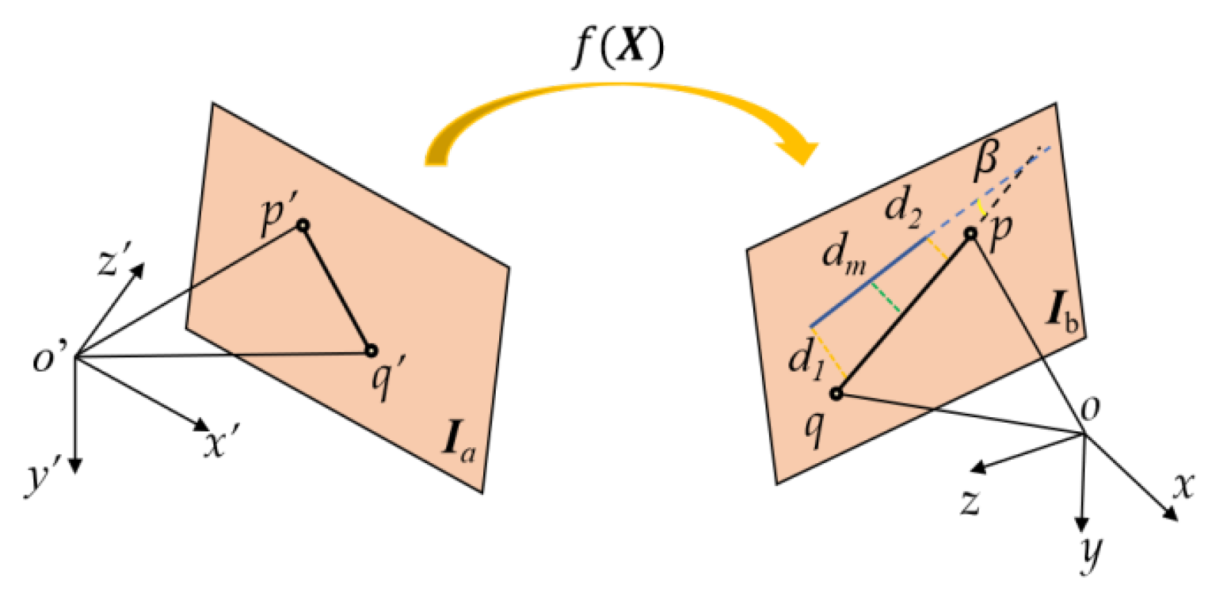
Fourier representations facilitate the establishment of a mapping relationship between pairs of images. Enhancing local geometric constraints is essential for achieving precise matching pairs [13]. In this study, constraints were introduced and integrated into the posterior probability model to ensure the accuracy of matches. Figure 2 depicts three types of geometric constraints employed in the proposed line feature matching algorithm for adjacent images (Ia, Ib): (i) the first constraint is denoted (d1, d2), which represents the distance from the endpoints of line features to their respective matched line; (ii) another term of distance constraint (dm) is established by the midpoint of matching line feature pairs; (iii) the angle constraint refers to the angle between matching lines, which is denoted as β in Figure 2. In our study, the geometric constraints are designated as Condition A, Condition B, and Condition C, respectively.
Condition A: As shown in Figure 2, the re-projection constraint on endpoints of the line feature requires that, after applying the transformation model f(X) based on the Fourier representation between image pairs, the distances (d1, d2) from each endpoint of the line feature to its corresponding line feature are to be minimized. The formula for calculating this constraint is presented as follows:
d 1 = | a · u s + b · v s + c | d 2 = | a · u e + b · v e + c | ,
where (a, b, c) are the coefficients of the linear equation on the 2D image coordinate system, and it satisfies a · a   +   b · b = 1. (us, vs, 1) and (ue, ve, 1) represent the homogeneous coordinates of two endpoints on the line feature.
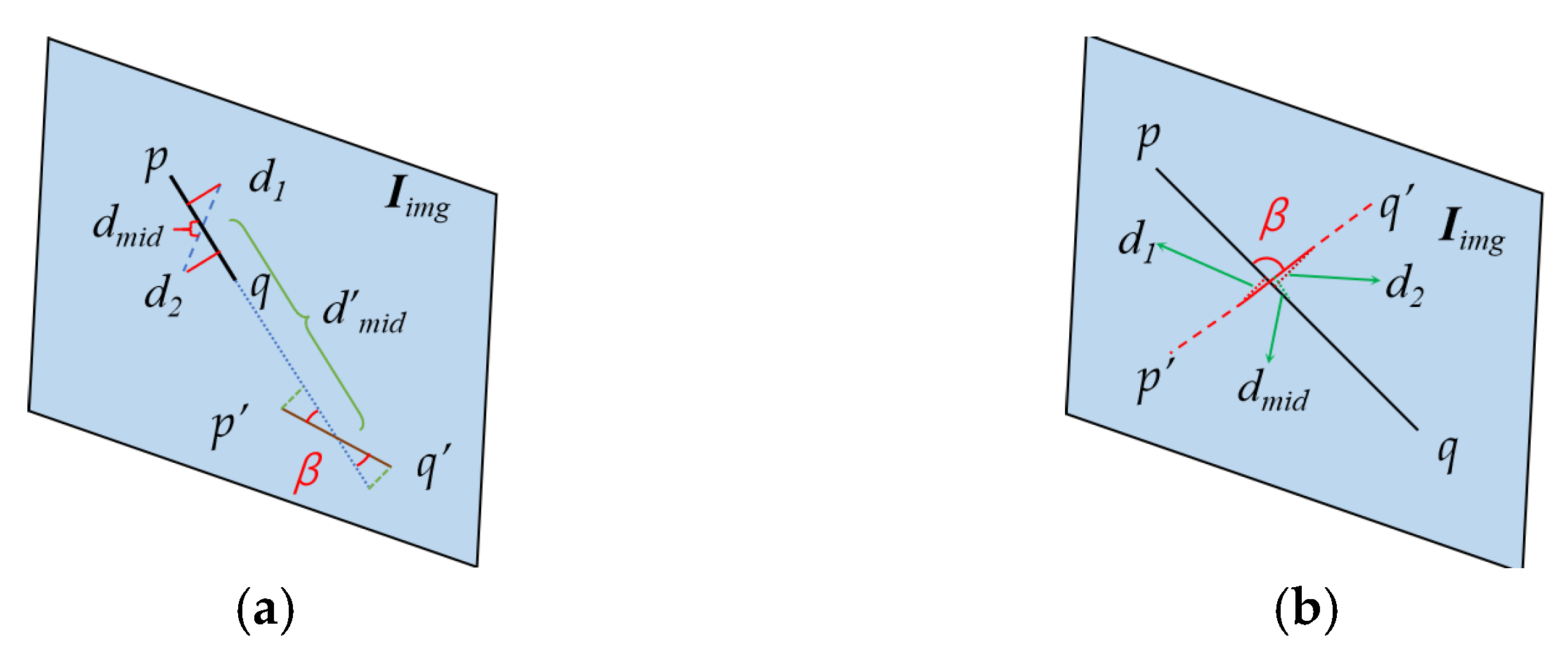
Condition B: As depicted in Figure 3a, the midpoint distance constraint for line features stipulates that, after transforming the matched line feature pair into the 2D image space, the distance between their midpoints is to be minimized. This midpoint distance is quantified as the Euclidean distance computed by applying the homogeneous coordinates of the line feature endpoints:
d m = | | X m I a X m I b | |
where X m I a and X m I b represent the homogeneous coordinates of the midpoint of the line feature in the image pairs Ia and Ib, | | | | represents the norm operation of the vector.
Condition C: As shown in Figure 3b, the angle constraint ensures that, after the transformation, the angle between the matched line feature pairs meets a preset threshold. This angle value is determined by applying an inverse trigonometric function to the radian value obtained from the vectors' dot product:
a r c c o s   β = < L 1 , L 2 >
where (L1,L2) represents the line feature equation expression on the image, and <,> is an operating symbol to calculate the included angles by vectors. Only when the three conditions mentioned above meet the intersection conditions Condition A, Condition B, and Condition C can they be considered as correct matching pairs of line features.

3.3. Posterior Probability Estimation via Expectation–Maximization Algorithm

To make a robust estimation of f ( X ) in the existing outliers of line feature matching, we make the following reasonable assumptions about the correspondence of line feature matching: (i) line feature matching pairs exhibit independent and identically distributed relationships; (ii) for the correct line feature matching pairs, each feature matching pair white noise satisfies the Gaussian zero mean and uniform standard deviation σ; (iii) for any line feature matching pairs, yn satisfies a random distribution in the bounded region in the R D , and its distribution is uniform 1/a and represents the region volume. The hidden variable zn ϵ {0, 1} denotes the nth matching pair of corresponding line features (xn, yn), where zn = 1 indicates that the matching pair is a correct match, otherwise it can be a mismatch. In addition, each latent variable zn conforms to a discrete distribution, i.e., p(zn = 1)= γ, p(zn = 0) = 1 − γ, where γ ∈ [0, 1]. Let X = [x1, x2, ..., xn] and Y = [y1, y2, ..., yn]T be the location data and measurements, then the joint probability distribution is expressed as
p l i n e ( Y | X , θ ) = n = 1 N z n p l i n e ( y n , z n | x n , θ )
where θ = { f , σ 1 , σ 2 , γ } denotes a series of unknown variables in the likelihood probability distribution.   σ 1   denotes the variance of the distance between endpoints in matched pairs of line features, while   σ 2 represents the variance in distances between midpoints of matched pairs of line features. xn represents two endpoint coordinates of line feature on the current image, and yn refer to the endpoint coordinates corresponding to the initial matching image, which could be obtained from the distance constraint from endpoint to the line segment. As per Equation (6), the first two line feature constraint conditions can be specified as follows:
p l i n e ( Y | X , θ ) = n = 1 N ( γ ( 1 ( 2 π σ 1 2 ) D / 2 e | | ( a i , b i , c i ) ( f ( X i ) , 1 ) | | 2 2 σ 1 2 + 1 ( 2 π σ 2 2 ) D / 2 e | | d m i ) | | 2 2 σ 2 2 ) + 1 γ s )
where D represents the data dimension, f ( X ) is the line feature matching pair expression after applying the Fourier mapping transformation, γ denotes the regularization weight coefficient,   d m i   is the midpoint distance, and (ai, bi, ci) represents the mathematical expression of the line equation. s represents the regularization factor term.
For the angle between the line feature matching pairs, the algorithm computes the line feature angle by using Equation (8). Here, [a, b, c] and [a′, b′, c′] represent the linear equations of the matched line feature pair. The result of the line feature angle constraint is modeled as a uniform distribution. We calculate the probability of the ith line feature matching pair based on the angle constraint Condition C and uniform distribution and denote it as p i C .
L i n e a n g l e = a c o s d ( a , b , c ) · ( a , b c ) | | ( a , b , c ) | | · | | ( a , b , c | |
According to Bayesian rule, the hidden variables have a prior distribution, and the maximum posterior probability (MAP) is estimated as
θ * = arg max θ   p l i n e ( θ | X , Y ) = arg max θ   p l i n e ( Y | X , θ ) p l i n e ( θ )
After performing logarithmic operations on both sides of the equation, Equation (9) becomes
θ * = l n p l i n e ( θ ) n = 1 N l n z n p y n , z n x n , θ .
We address latent variables in the posterior probability distribution of line feature matching pairs by employing the EM algorithm [51]. The iterative process comprises two steps: the expectation step (E-step) and the maximization step (M-step). We further expand Equation (10) to derive the following parameters:
Q ( θ , θ o l d ) = 1 2 σ 1 2 n = 1 N p i A ( | | ( a i , b i , c i ) ( f ( X i ) , 1 ) | | 2 ) 1 2 σ 2 2 i = 1 N p i B ( | | d m i | | 2 ) D 2 l n σ 1 2 n = 1 N p i A D 2 l n σ 2 2 n = 1 N p i B + l n ( 1 γ ) n = 1 N ( 1 p i A p i B ) + l n γ n = 1 N ( p i A + p i B ) l n p A ( θ ) l n p B ( θ )
where   θ represents the posterior probability of the variable, θ o l d denotes the variable before updating. p i A and p i B denotes the probability of the hidden variable z n within the ith line feature based on Condition A and Condition B. The EM algorithm is divided into two steps; the first step is the expectation step.
E-step: The current parameter value θ o l d is used to find the posterior distribution of the latent variable. By using the Bayesian rule, p i A or p i B can be calculated as follows:
p i A = γ ( e | | ( a , b , c ) ( f ( X ) , 1 ) | | 2 2 σ 1 2 ) γ ( e | | ( a , b , c ) ( f ( X ) , 1 ) | | 2 2 σ 1 2 ) + ( 1 γ ) ( ( π σ 1 2 ) D / 2 s )
p i B = γ ( e | | d m | | 2 2 σ 2 2 ) γ ( e | | d m | | 2 2 σ 2 2 ) + ( 1 γ ) ( ( π σ 2 2 ) D / 2 s )
M-step: The modified parameter estimation step is updated using following equation, and the updated parameter of sum can be calculated by deriving Equation (9) and making its left value 0. Here, each p l i n e A or p l i n e B is written as a diagonal matrix, then the derivative of Equation (9) is
σ 1 2 = t r ( M T P M ) D · t r ( P ) ,   σ 2 2 = t r ( J T Q J ) D · t r ( Q )
γ = t r ( P + Q ) N
Let l i = | | ( a i , b i , c i ) ( f ( X i ) , 1 ) | | 2 , j i = | | d m i | | 2 , where M = [ l 1 , l 2 , , l n ], J = [ j 1 , j 2 , , j n ] N is the dimension of the pointing quantity, in the case of P = diag( p 1 A , p 2 A , , p n A ), Q = diag ( p 1 B , p 2 B , , p n B ) as a diagonal matrix, p i A and p i B represents the probability that the ith line feature matches correctly based on Condition A and Condition B. tr(.) represents the trace of the matrix.
The final probability for the matching pair is determined by combining this angle probability with two other probabilities mentioned above. Finally, the ith line matching pairs are screened using a set threshold p s e t , and this final probability p i is calculated in Equation (16). To retain as many line matching pairs as possible, we set the probability p s e t to 0.70 based on our actual experimental results. Considering the error factors in image line feature detection and geometric constraint probability models, combined with our practical experience, ω 1 , ω 2 , and ω 3 are set to 0.4, 0.4, and 0.2, respectively.
p i = ω 1 · p i A + ω 2 · p i B + ω 3 · p i C ,     ω 1 + ω 2 + ω 3 = 1
Next, we consider updating the function f(X) from Equation (1). We assume flat priors for σ 1 , σ 2 and γ; thus, pline(θ) degrades following functional into p(f). By abstracting the terms related to f, we obtain the following functional:
ε ( f ) = 1 2 σ 1 2 n = 1 N p l i n e A ( | | ( a , b , c ) ( f ( X i ) , 1 ) | | 2 ) 1 2 σ 2 2 n = 1 N p l i n e B ( | | d m i | | 2 ) l n   p l i n e A ( f ) l n   p l i n e B ( f )
As aforementioned, the f function has a as coefficients with random distribution, and the term −ln p(f) can be denoted as a i T R 1 a i . Consequently, with λ > 0 as a predefined parameter, the following objective problem can be obtained:
min ε ( f ) = 1 2 σ 1 2 n = 1 N p l i n e A ( | | ( a , b , c ) ( f ( X i ) , 1 ) | | 2 ) 1 2 σ 2 2 n = 1 N p l i n e B ( | | d m i | | 2 ) + λ a i T R 1 a i
To increase the number of line feature matches, we obtain the existing line feature matching set L i n e s e t c u r after completing the line feature matching based on EM solution algorithm. The existing line matching pairs satisfy the Fourier representation transformation model f ( ) and the posterior probability distribution model we constructed. Because of the influence of the noise parameters of the initial model, there may leave some straight-line features that are not matched denoted L i n e s e t a d d . To supplement this line matching set, we search for extra matches among the remaining candidate line features, resulting in a line matching set L i n e s e t n e w :
L i n s e s e t n e w = L i n e s e t a d d L i n e s e t c u r
Then, the new matching set L i n s e s e t n e w satisfies the posterior probability distribution:
p l i n e n e w ( Y | X , θ ) , X L i n e s e t n e w
Combining the previous parameter values and Equations (11) and (20), the iteration is updated again until the number of line feature matching pairs does not increase.

4. Experimental Verification and Performance Analysis

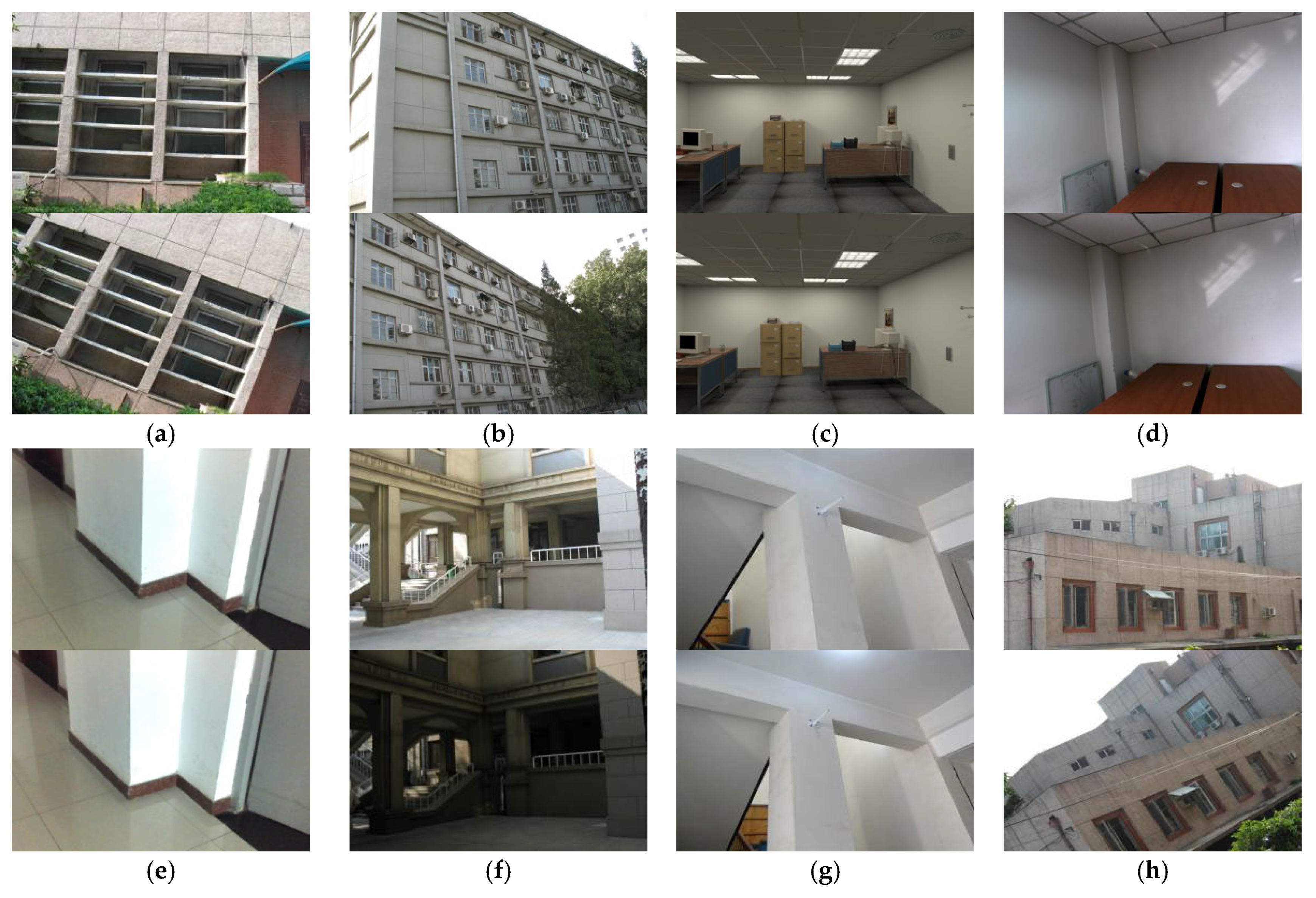
To thoroughly evaluate our algorithm’s effectiveness, we selected multiple groups of line feature matching pairs from some datasets or data sequences: a public dataset [52], the SLAM indoor low-texture data sequence [53] (refer to Figure 4). The datasets encompass diverse scenarios, particularly under low-texture, rotation, view-changing and variable illumination conditions, satisfying our experimental requirements. The experimental section of this paper is structured into seven subsections: (1) configuration of experimental parameters; (2) line feature matching comparison among our and other algorithms; (3) ablation study and component analysis; (4) comparison analysis with deep learning-based line feature matching algorithms; (5) comparative verification of line feature matching based on descriptor; (6) line feature matching in illumination-sensitive scenarios; (7) sparse 3D reconstruction using our line feature matching results; and (8) comparative time efficiency evaluation. To quantitatively evaluate performance, we introduce the variable MP to represent the matching pairs:
M P = M C / M .
where M is the total number of matched line feature, MC is the number of correct matches.

4.1. Experimental Parameter Configuration

In this section, we used the LSD algorithm to detect and extract line features and then calculated the corresponding descriptors using the function interface provided by OpenCV. The relevant parameters involved in the algorithm are explained as follows:
(i)
T is the number of basis functions in Equation (1); we determine the optimal parameter by evaluating image pairs (a), (c), (d), (f), and (h) individually. Through our experimental observations, it was established that an insufficient number of basis functions (T < 5) compromises the robustness of representing relationships between image pairs, while an excessive number (T > 15) may lead to overfitting, catering to only specific cases of image matching pairs. Consequently, T was constrained to a range of 5 to 15. The outcomes depicted in Figure 5 revealed that T between 11 and 15 yielded a relatively low number of matching pairs, whereas T between 5 and 9 showed an increase in line matching pairs. Notably, setting T to 10 nearly maximized the selection of image line matching pairs. Considering the collective findings from our experiments, a final decision was made to set T at 10.
(ii)
The parameter σ (including   σ 1 , σ 2   , here, we will synchronize the two with incremental increases, using σ to represent both) is the initial distance variance of the line feature matching pair. Based on the image pairs (a), (c), (d), (f) and (h),   σ   range from 0.1 to 1.0. By comparing the line feature matching results across different σ in Figure 5, it is observed that setting σ to 0.3 yields the maximum number of line feature matches for the selected image pair under a fixed T value. Therefore, the parameter is set to 0.3 in our study.
Figure 5. Variation in the number of line feature matches with different T and σ .
Electronics 14 03783 g005
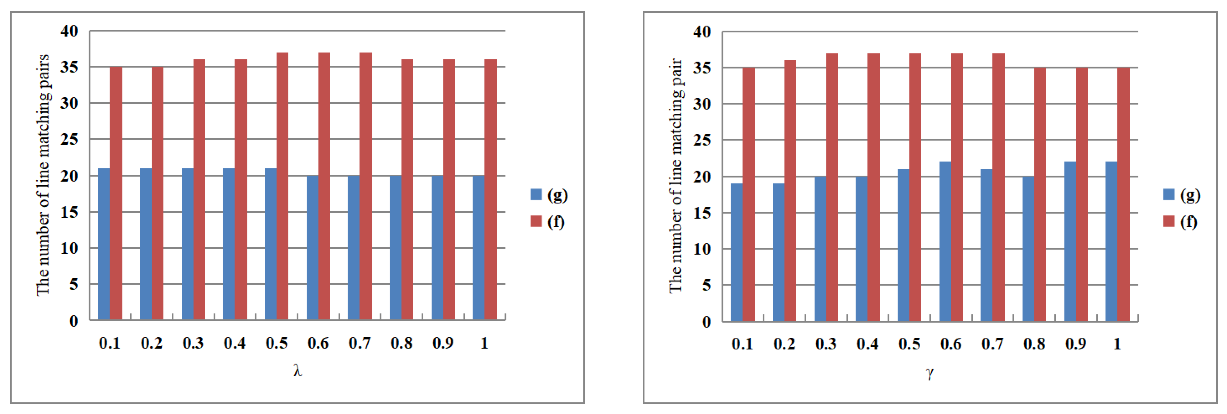
The equilibrium factor of regularization, denoted as λ, is determined based on the image pairs (a), (c), (d), (f), and (g). Experimental tests were conducted within the range of λ ∈ [0.1, 1.0], where the number of line feature matching pairs (a), (c), and (d) remain constant. Figure 6 displays the experimental results for selected image pairs (g) and (f). Examination of image pairs (f) and (g) indicated a fluctuation in the number of line matching pairs across the λ range of [0.1, 1.0]. Based on our actual experimental results, a λ value of 0.5 was selected.
γ represents the internal proportions of the corresponding set of the following initial assumptions and on the basis of the parameter λ. In this study, we systematically varied γ from 0.1 to 1 using image pairs (a), (c), (d), (f), and (g). when the γ ∈ [0.1, 1.0], the number of line feature matching pairs (a), (c), and (d) is constant. The number of matched pairs for image pairs (g) and (f) is presented in Figure 6. Notably, based on the results obtained from image pairs (g) and (f), the line feature matching accuracy was found to be highest when γ was set to 0.6, as confirmed by experimental validation.

4.2. Line Feature Matching Comparison Among Our and Other Algorithms

For comprehensive evaluation, we implemented and compared multiple state-of-the-art line-matching approaches. Firstly, we reproduced the “Point + Line” invariant method [40], which establishes novel geometric constraints by combining SIFT point features with LSD line features to compute homography transformations. Additionally, we included two other prominent algorithms: Line Junction Line (LJL) [32] and Hybrid Matching [35], both known for their robust performance across diverse scenarios. Our comparative analysis employed eight challenging image pairs (a)–(h), with detailed findings outlined in Table 1. Within the table, bold values denote superior performance, while dashes (“—”) indicate cases where algorithms failed to produce valid matches. The experimental results reveal that while all three comparison methods achieve competitive results in standard conditions, each exhibits distinct limitations in challenging cases.
The results presented in Table 1 indicate that our method outperforms existing approaches in 60% of the test cases (five out of eight image sequences) while maintaining competitive performance in the remaining data sequences. In contrast, the algorithm described in Reference [40] fails to produce satisfactory results for image pairs (b) and (e) due to its fundamental reliance on point–line feature invariants. This approach proves particularly ineffective in low-texture scenarios where insufficient feature points are available for reliable invariant construction, resulting in either a significant reduction in matches or complete failure in matching. Among the benchmark methods, the Hybrid Matching approach [35] exhibits inconsistent performance, failing entirely on specific image pairs (e.g., (a)–(b)) while delivering only moderate results in other cases. The LJL algorithm [32], while achieving overall success in experiments and displaying robustness, suffers from substantially higher computational demands, making it less practical for time-sensitive applications.
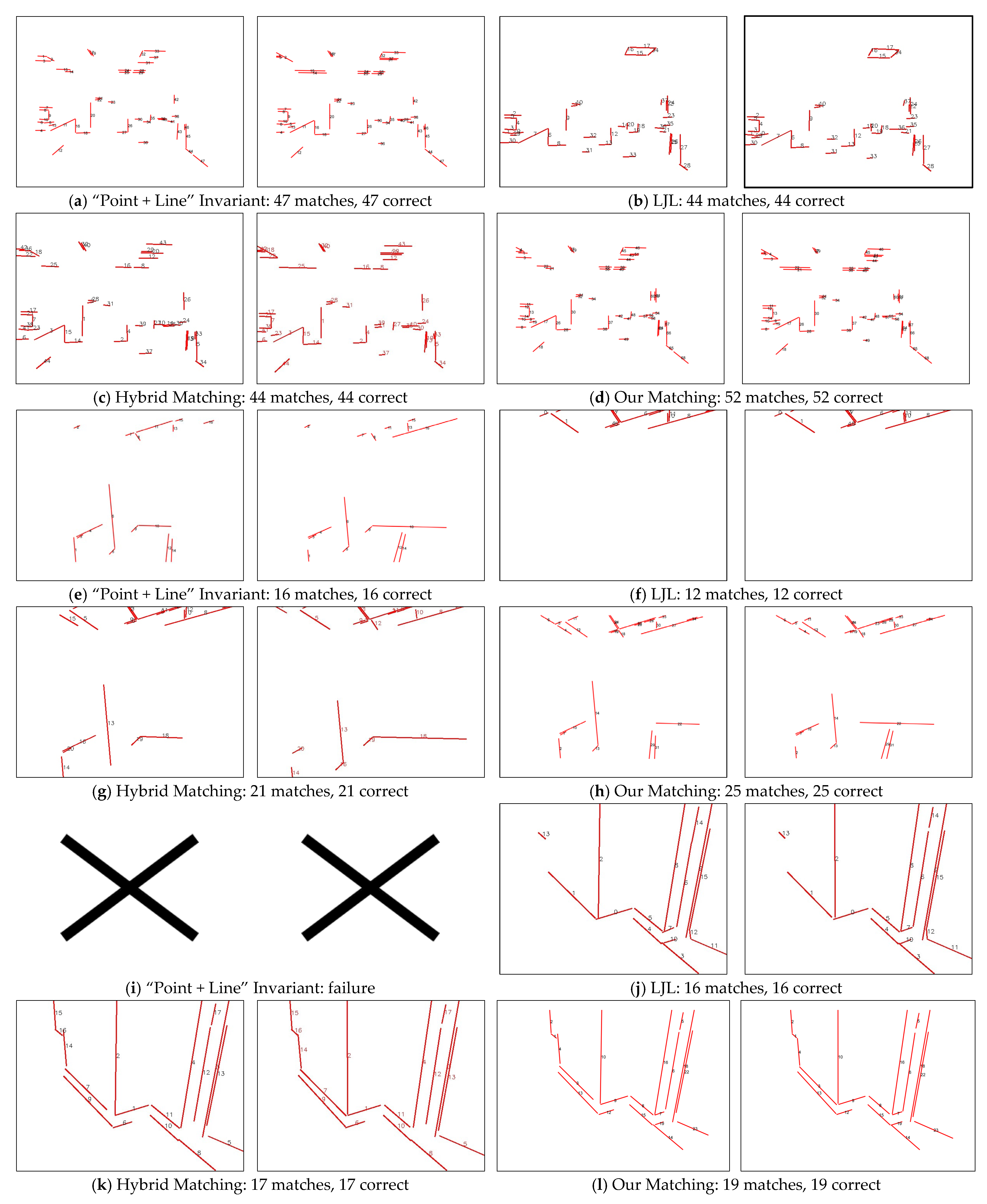
Figure 7 visualizes the matching results of line feature algorithms, including the “Point + Line” invariant matching method [40], LJL [32], Hybrid Matching [35], and our proposed approach. Images (a)~(h) show the matching results under indoor low-texture and weak-texture scenes, respectively. In these scenes, sparse and uniform textures pose challenges. The “Point + Line” invariant method [40] relies heavily on accurate point feature matching. However, repeated textures often complicate point matching, leading to fewer successful invariant-based matches. However, repeated textures in such scenes can complicate point feature matching, and the line feature-based invariant construction may result in fewer successful matches. The LJL and Hybrid Matching algorithms require homography matrices to filter candidate line feature matches. The accuracy of this homography estimation directly influences line-matching performance and increases computational time.
In contrast to existing approaches, our algorithm does not depend on point features or require the computation of homography matrices. It exclusively employs a binary descriptor for line features to filter out mismatches. Moreover, the algorithm effectively incorporates geometric constraints within a posterior probability model, leading to markedly enhanced performance compared to the methodologies outlined in the cited literature [32,35,40].

4.3. Ablation Study and Component Analysis

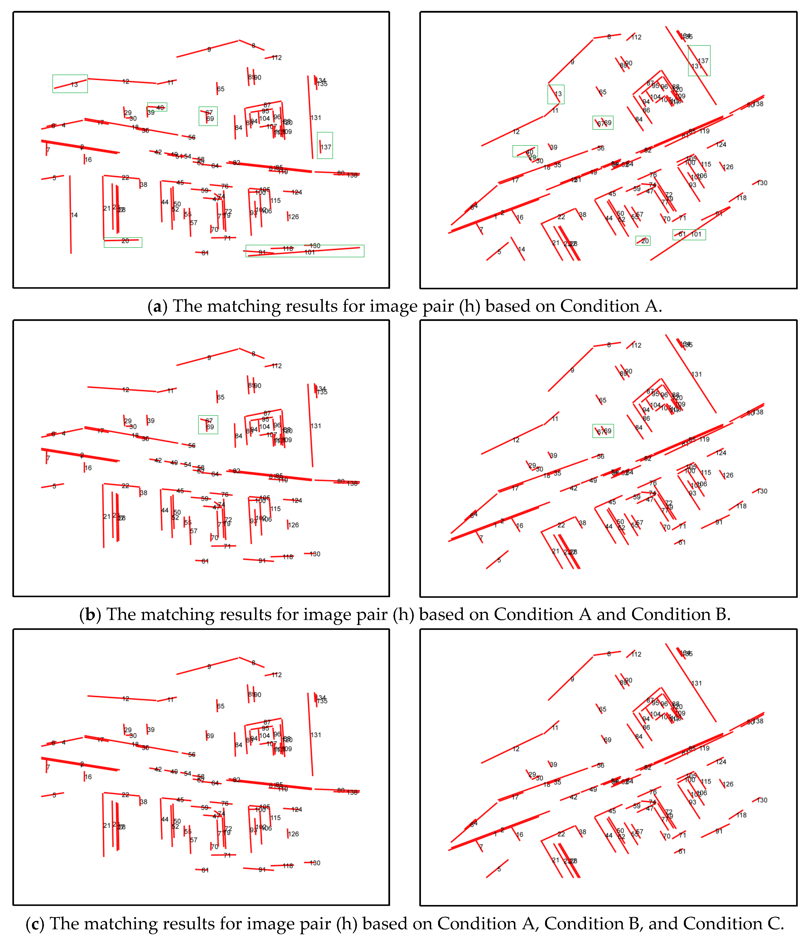
To validate the effectiveness of three geometric constraints for line feature matching, we conducted ablation experiments with qualitative and quantitative comparisons. We conducted these experiments on sparse-texture, low-texture, and rotated image pairs to effectively showcase the proposed algorithm. Specifically, image pairs (c), (d), and (h) from the experimental dataset were selected for testing. The experiments were carried out by incrementally adding each of the three terms of constraints, and the results are summarized in Table 2. The quantitative comparison is still based on the matching performance (MP) as the evaluation metric.
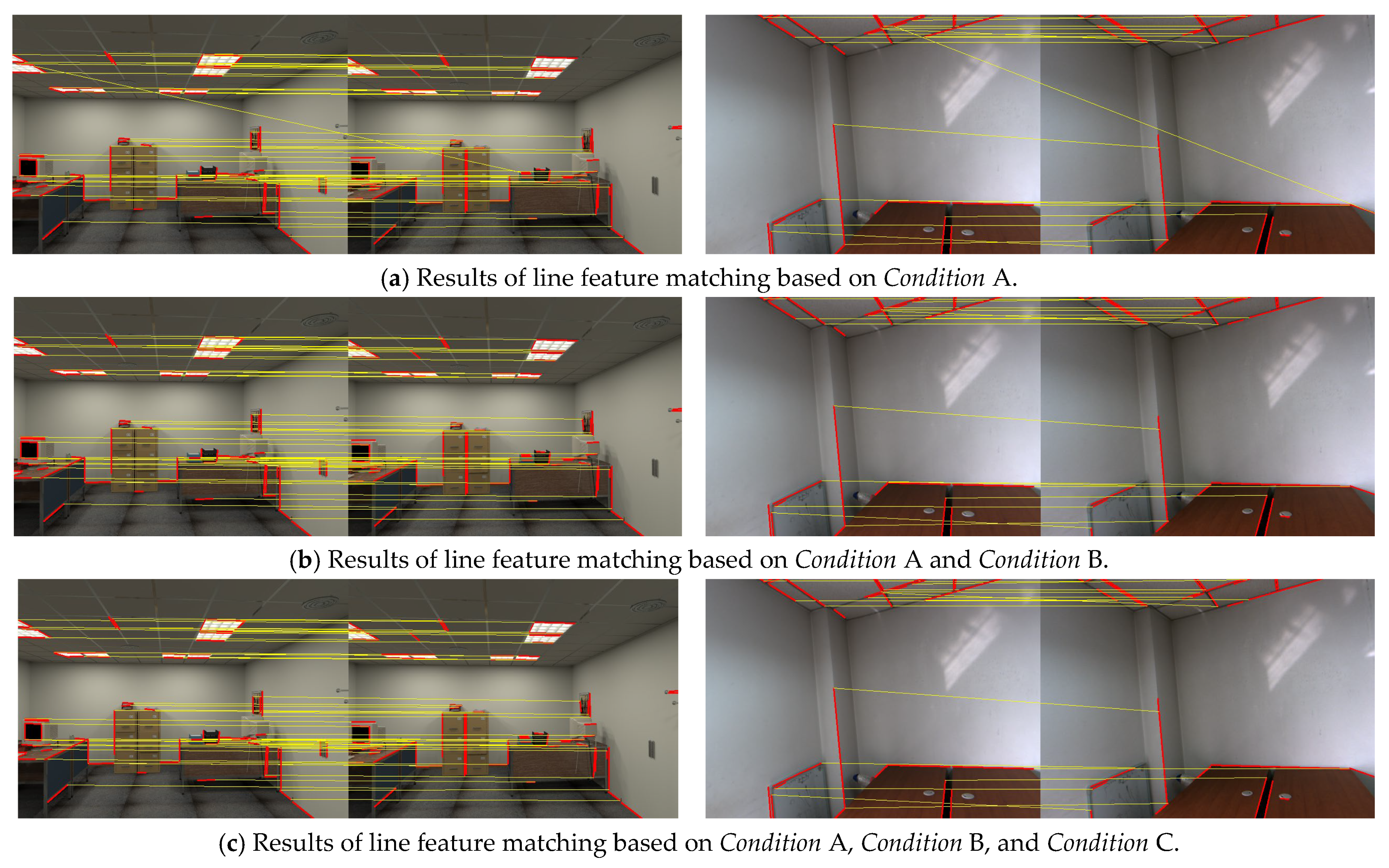
Combined with the ablation experimental results shown in Table 2, the proposed algorithm demonstrates a significant improvement in line feature matching accuracy. Specifically: Condition A yields a richer set of line features containing more inner lines. By adding geometric Condition B significantly reduces false positives, as evidenced in Figure 8. The inclusion of constraint Condition C further refines the line-matching results.
Figure 9 presents the corresponding visualization results for the three geometric constraint ablation experiments. Based on the constraint Condition A, there are 92 pairs of line feature matching pairs here, of which 6 pairs are mismatched. These mismatched pairs are marked by green rectangular boxes in Figure 9a. By jointly constraining Conditions A + B, the accuracy of line matching has been improved. Among the 85 pairs of line feature matching pairs, only one pair is a mismatch, which is also marked by the green rectangular box in Figure 9b. Although the mismatched pairs in Figure 8b satisfy the constraint conditions A and B, the angle is almost 90 degrees, which does not meet the angle constraint condition. After adding the term angle constraint condition, it effectively removes the mismatches. It is not difficult to prove the effectiveness and robustness of the proposed algorithm from the above ablation experiment results.

4.4. Comparative Analysis of Deep Learning-Based Line Feature Matching

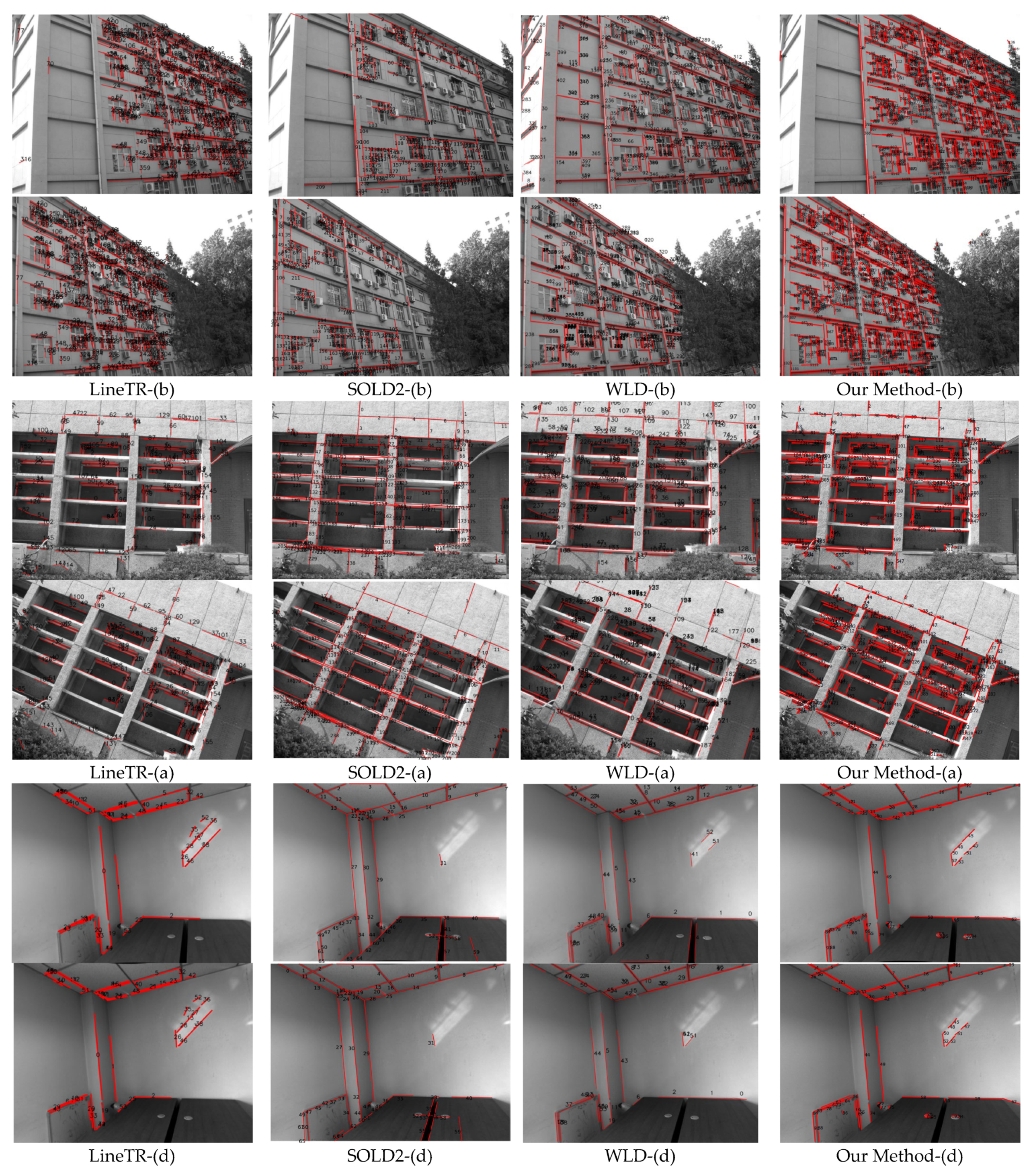
In the section, we conducted a thorough comparison between our proposed method and three existing deep learning-based approaches for line matching (SOLD2 [44], LineTR [45], WLD [47]). LineTR treats line feature as a sequence of points, emphasizing point features along the line to generate variable-length line descriptors. It utilizes attention mechanisms to enhance cross-view line feature correspondence. WLD employs wavelet transformation to extract line features from images and utilizes a deep learning model for feature description and matching. SOLD2 is a deep learning network model designed for detecting and describing joint learning segments. It introduces a self-supervised network that can be trained on any image dataset without labels. These deep learning-based line feature matching algorithms are widely used and exhibit high robustness; hence, we selected them for comparison with our algorithm. For fairness, all methods were tested on image pairs (a)–(h) employing the raw LSD detector. In the results, as presented in Table 3, entries marked with “—” indicate insufficient correct matches, whereas “×” signifies a low MP indicator, leading to the algorithm being deemed unsuccessful.
The experimental results shown in Table 3 demonstrate that SOLD2 yields a higher number of successfully matched line features, displaying superior performance in 50% of the image pairs tested. In contrast, its performance significantly deteriorates under more challenging conditions, such as significant viewpoint changes (e.g., image pair (b)) or extreme rotational shifts (e.g., image pair (a)). While LineTR shows a satisfactory overall matching performance, it tends to generate a relatively low number of matched line feature pairs, which may be limiting in specific applications (e.g., visual location). On the other hand, the experimental outcomes of WLD reveal unsatisfactory matching results for image pairs (a), (b), (f), (g), and (h), characterized by numerous incorrect line segment matches, leading to the algorithm’s failure in these instances. In comparison, our proposed algorithm, although slightly trailing certain deep learning-based methods (SOLD2) in matching performance, presents notable practical advantages. It operates independently of specialized hardware and exhibits superior adaptability across various scenarios compared to both LineTR and WLD. Notably, while the absolute count of matched line features may occasionally be lower than that of deep learning techniques, our method consistently maintains higher matching precision.
Figure 10 presents the line feature matching performance across several typical scenarios. Notably, three algorithms demonstrate markedly reduced accuracy when processing image pairs (a) and (b). In contrast, our approach sustains superior robustness when confronted with significant viewpoint changes and rotational transformations. Our algorithm, along with SOLD2, demonstrates superior performance in pair (d) when compared to LineTR and WLD. While the results of the SOLD2 algorithm in Table 3 are promising and satisfactory, its matching outcomes in pairs (a) and (b) do not match the performance of our algorithm. Furthermore, in pair (d), although our results exhibit a slight edge over the SOLD2 algorithm, the latter is susceptible to inaccurate line segment detections (e.g., line feature matching label 59 and 21 in the image pair (d) of SOLD2), a shortcoming not observed in our algorithm.

4.5. Comparative Verification of Line Feature Matching Based on Descriptor

To further verify the effectiveness and robustness of the line feature matching algorithm in this paper, the matching experimental results of feature matching are also compared with this matching method based on descriptor (LBDfloat + FLANN (i.e., Fast Library for Approximate Nearest Neighbors), LBDbinary + FLANN). In Reference [34], a line descriptor (ILLB) aiming at illumination variation scene was designed and showed strong robustness for the line feature matching. Based on the descriptor, we carried out corresponding comparative experiments with the descriptor for feature matching; the list of comparative experimental results is in Table 4 below.
Table 4 presents a comparative analysis of matching methodologies. Our approach employs bidirectional descriptor matching to establish initial correspondences, which are subsequently refined through pairwise similarity evaluation. This differs fundamentally from Reference [34], which implements length-based filtering during line feature extraction—a process that substantially decreases the quantity of viable matches compared to our direct application of LSD extraction. The quantitative results clearly demonstrate the superiority of our method over Reference [34]’s IILB descriptor, with significant improvements in both matching pair quantity and matching precision (MP) metrics.

4.6. Line Feature Matching in Illumination-Sensitive Scenes

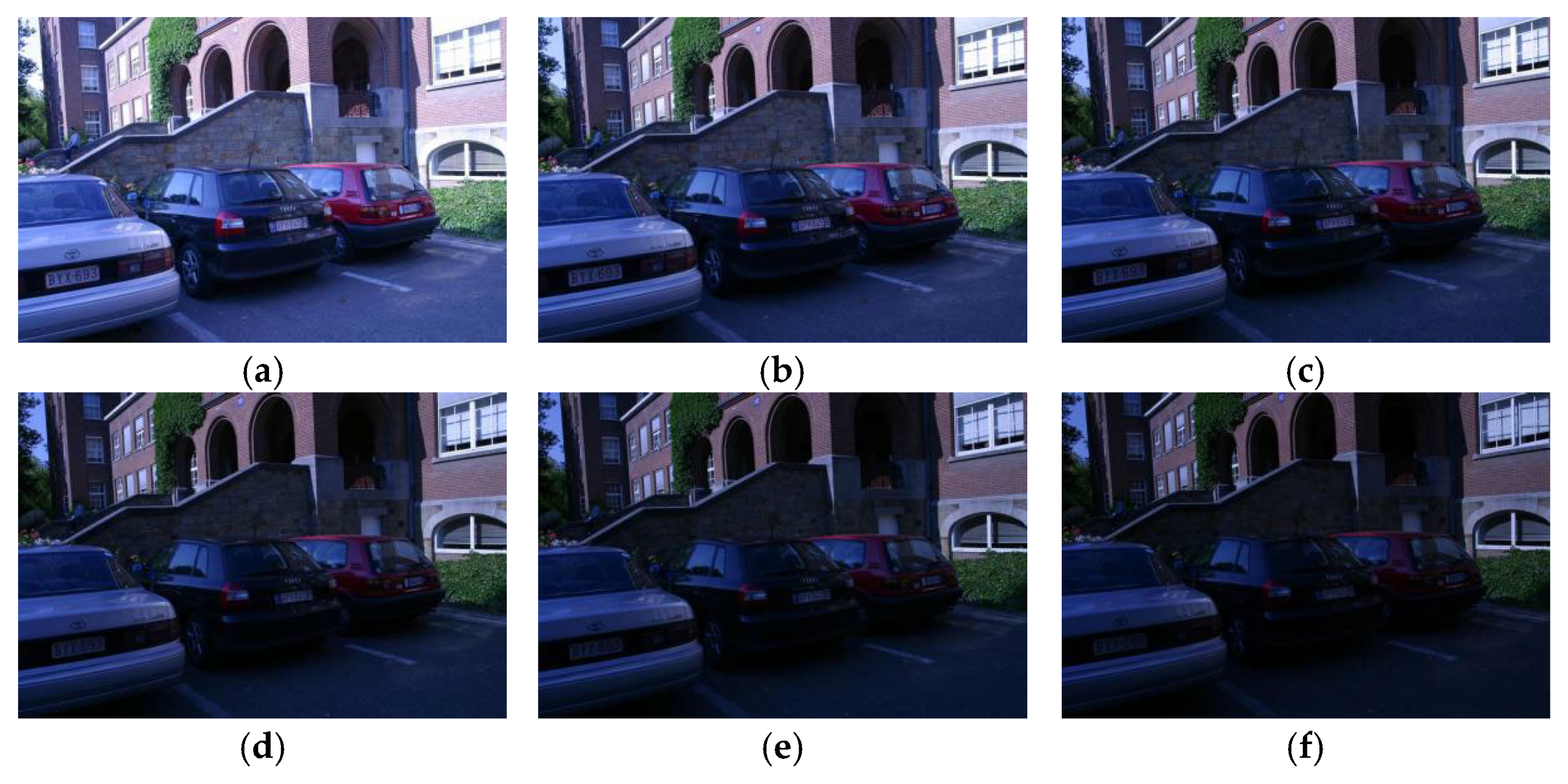
To assess matching performance under different lighting conditions, we conducted comparative experiments on the IILB descriptor [34], which was specifically developed for light-sensitive scenarios. Six image pairs (labeled (a)–(e) in Figure 11) from the image sequence were analyzed to represent various lighting variations. Each test case pairs the reference image (a) with subsequent images (b–f) exhibiting progressively stronger illumination changes. Quantitative results presented in Table 5 employ the MP metric to evaluate matching performance, highlighting our method’s enhanced robustness in challenging lighting situations compared to the specialized IILB technique.
The experimental results in Table 5 demonstrate our matching pipeline, where initial candidate pairs are generated through bidirectional descriptor matching and subsequently refined via pairwise similarity evaluation. Unlike Reference [34], which employs length-based filtering of LSD-extracted features leading to substantially fewer matches, our approach utilizes unfiltered LSD line features to preserve matching opportunities. As evidenced by the quantitative comparison in Table 5, our method outperforms the IILB descriptor across both evaluation metrics—yielding more correct feature correspondences while maintaining superior matching precision (MP).

4.7. Sparse 3D Reconstruction Using Our Line Feature Matching Results

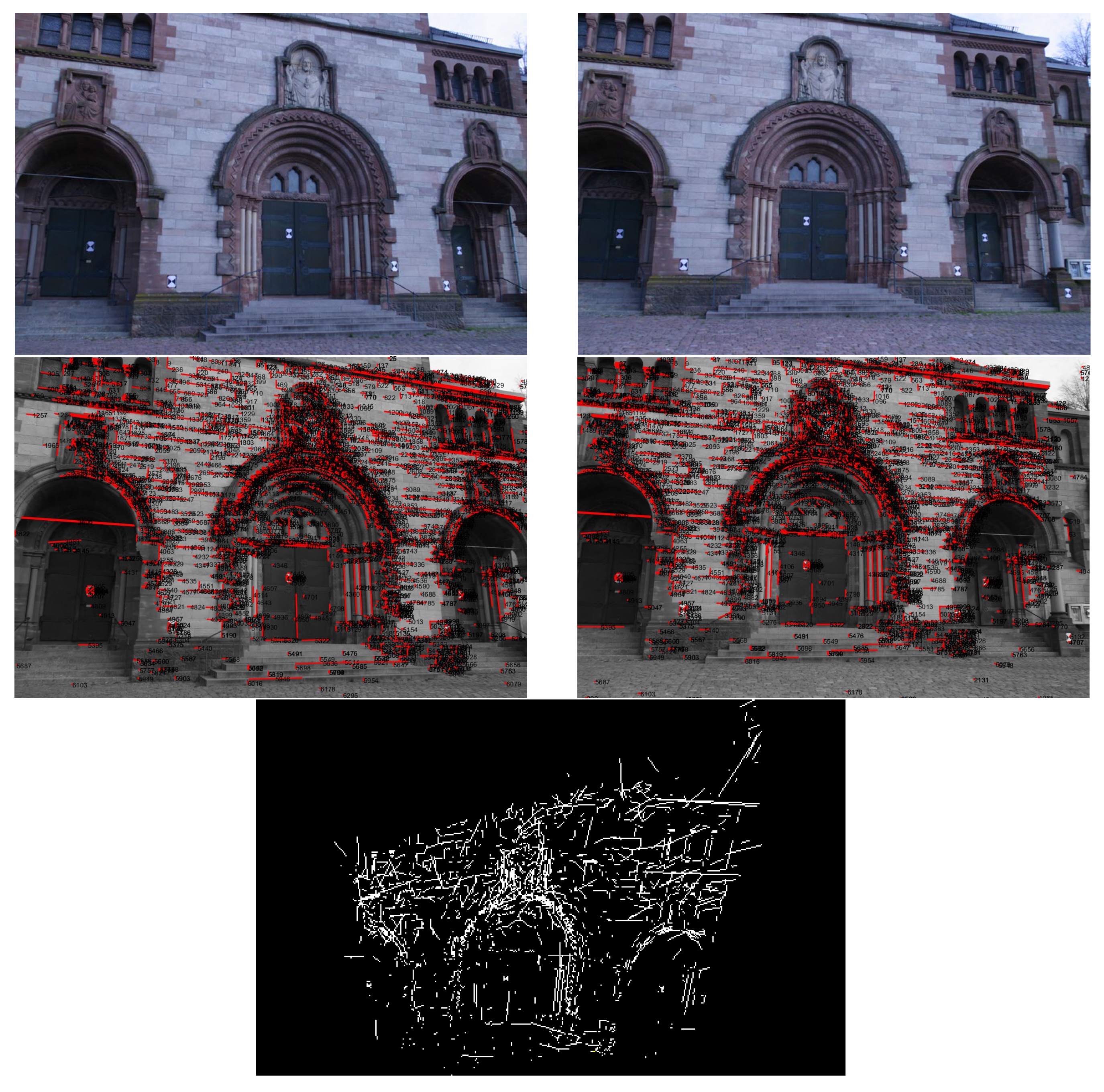
The matching results of line features play a vital role in the precise construction of three-dimensional models using structural information. They greatly improve the geometric integrity, structural accuracy, and visual fidelity of the reconstructed model. As such, we reconstruct three-dimensional line segments based on the matching results of line features to indirectly validate our method. We conducted experiments using the high-resolution Herz-Jesu dataset [54] to validate the practical applicability based on our line feature matching method. Image samples were chosen from the Herz-Jesu dataset based on its high-resolution ground images. The texture features on these high-resolution ground images are quite similar, and the surface structures are irregular, which poses significant challenges for line feature matching. Subsequently, line features were extracted on these images, and three-dimensional line features were reconstructed based on our line feature matching results set. The Herz-Jesu example image and the corresponding line feature matching outcomes are depicted in Figure 12. These results demonstrate that our algorithm effectively captures scene structure information through line features, thereby facilitating the 3D reconstruction of the scene.

4.8. Comparative Time Efficiency Evaluation

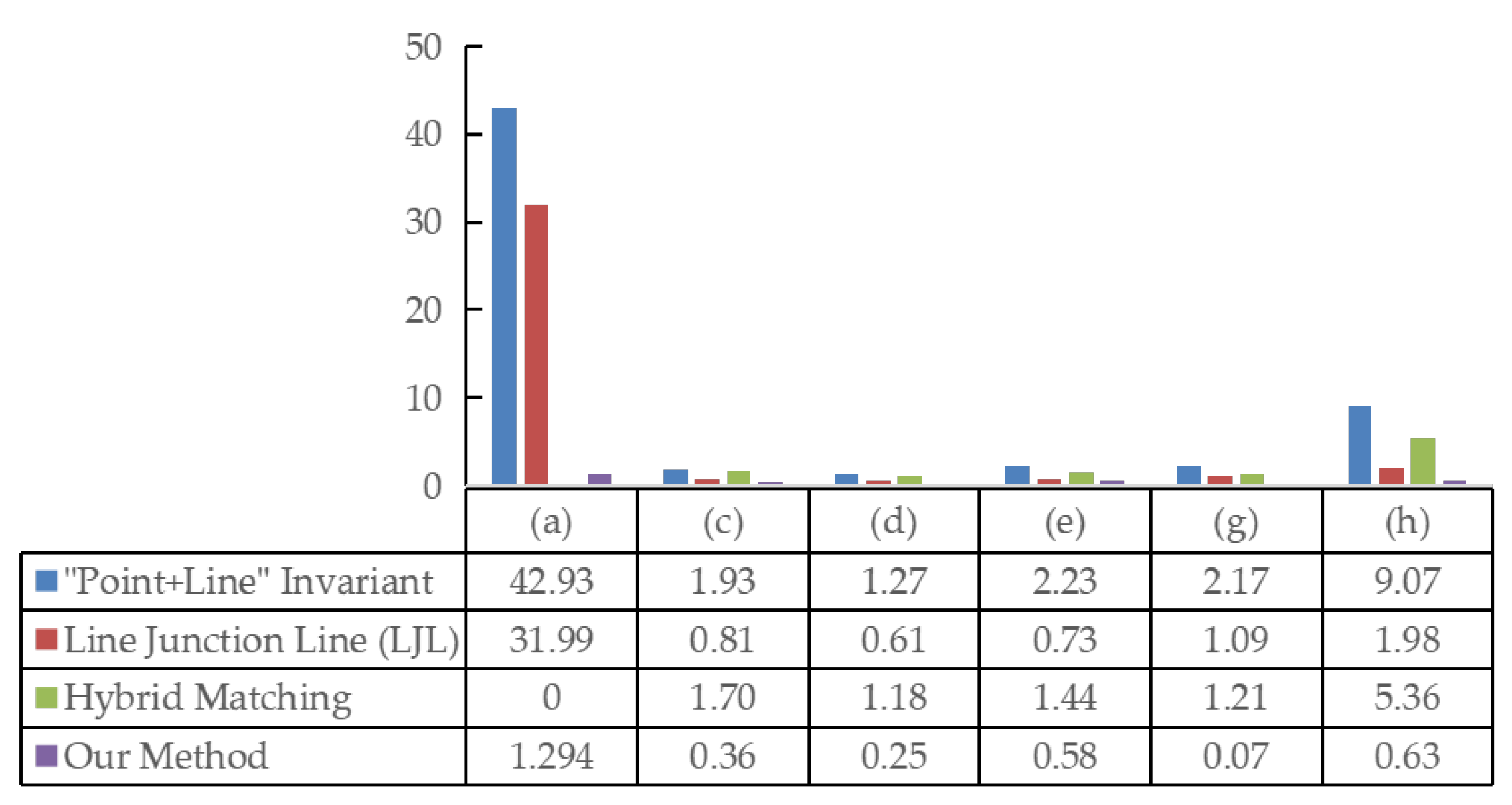
We studied and analyzed the time efficiency of these algorithms, and the experiment still uses the image pairs (a), (c), (d), (e), (g), and (h). In the image pair (a), the line-matching pair obtained by the algorithm proposed in Reference [35] is denoted as “—“, and it means the algorithm failed to perform on this specific image pair. It is direct to find from Figure 13 that compared with References [32,35,40], in which these proposed algorithm experiments with feature matching by calculating the homography matrix, the time consumed in our proposed algorithm is significantly less than their time consumed. The algorithm described in Reference [40] necessitates SIFT feature point detection, matching, point–line projection invariants establishment via point and line features, and single-response matrix computation based on point features to enhance the screening of line feature matching pairs, leading to its high time complexity. Similarly, LJL and Hybrid Matching algorithms require homography matrix calculations, contributing to their time consumption. In contrast, our method relies exclusively on line feature descriptors and accomplishes feature matching by constructing a posterior probability estimation model, eliminating the need for homography matrix filtration or point feature-assisted matching. Consequently, our algorithm significantly reduces computational time.

5. Discussion

While our method yields satisfactory matching results for the images under consideration in this study, it presents limitations when applied to specific image pairs. Our algorithm is based on minimizing outliers in matches through posterior probability estimation, akin to the well-established RANSAC concept [55]. Initially, the algorithm identifies matching pairs from line feature descriptors, which are less robust than point feature descriptors. Line feature descriptors can be affected by image scaling factors and pixel quality, unlike point features, thus hindering the matching of line features. In cases such as occlusions or flips, where feature descriptor pairs are ineffective for image matching, the lack of initial line feature matching pairs leads to algorithm failure. Additionally, the iterative nature of our posterior probability framework requires continuous parameter iteration and updating, making the framework unsuitable for all line feature match pairs, thus representing a limitation of the discussed algorithm. Going forward, our focus will be on investigating methods to dynamically adjust the posterior probability parameters to improve the algorithm’s applicability across different scenarios.
Our algorithm is less time-efficient compared to learning-based line feature-matching algorithms due to their dependency on robust hardware support and GPU acceleration. Our algorithm requires continuous iterative loops, resulting in notable time overheads. However, our experiments indicate that our algorithm competes effectively with specific learning-based line feature matching algorithms. Many of these algorithms necessitate training and labeling, exhibiting limited generalization capabilities. For example, the SOLD2 algorithm, despite being self-supervised, is vulnerable to line feature-matching degradation due to perspective changes in images, resulting in variations in line lengths and misaligned sampling points. In contrast, our algorithm utilizes descriptors and line feature detection algorithms for matching, thereby maintaining advantages in generalization and line feature detection matching.
Despite its limitations, our algorithm deserves recognition. The idea of RANSAC in point feature matching field is a widely accepted method, similar to our own approach. We have extended this concept to line features by introducing posterior sampling consistency, where line-matching pairs are continually iterated from initial line feature set, resulting in significantly improved line-matching results. Notably, our algorithm is pioneering in its utilization of probability sampling for matching line features, distinguishing it from most existing methods that rely on constraints like homography matrices or auxiliary point feature matching. This distinctive feature, combined with the algorithm’s high efficiency, represents its primary advantages.

6. Conclusions

We introduce a novel line feature matching algorithm that incorporates three geometric constraints: (1) endpoint distance, (2) midpoint distance, and (3) angular relationship between line pairs. Building upon the LSD line detector and its binary descriptor, our approach first establishes Fourier series transformation mappings between image pairs, then formulates these constraints into a maximum a posteriori (MAP) probability estimation framework for iterative line matching. Experimental results illustrate that our algorithm achieves superior performance compared to state-of-the-art methods (including those based on deep learning), particularly in challenging scenarios involving weak or low textures, rotational variations, and view changing. Additionally, our proposed method also demonstrates notable computational efficiency benefits. Future work will focus on enhancing Fourier-based inter-image relationships and implementing adaptive parameter updates within the matching framework.

Author Contributions

Conceptualization, C.Z. and Y.G.; methodology, C.Z. and Y.G.; software, C.Z. and Y.G.; validation, C.Z., Y.G., and S.G.; writing—original draft preparation, C.Z. and Y.G.; writing—review and editing, S.G. All authors have read and agreed to the published version of the manuscript.

Funding

This work was supported by the China Postdoctoral Science Foundation (No. 2023M741702), the National Natural Science Foundation of China (No. 42401533), and the Research Project of Basic Science (Natural Science) Research in Jiangsu Universities (No. 24KJB420002).

Data Availability Statement

The dataset can be found at https://github.com/zcyHHU/Line-Matching-Dataset (accessed on 9 May 2025), and the datasets all are collected by the camera.

Conflicts of Interest

The authors declare no conflicts of interest.

References

  1. Ding, Y.; Yang, J.; Ponce, J.; Kong, H. Homography-Based Minimal-Case Relative Pose Estimation with Known Gravity Direction. IEEE Trans. Pattern Anal. Mach. Intell. 2022, 44, 196–210. [Google Scholar] [CrossRef]
  2. Jiang, H.; Dang, Z.; Gu, S.; Xie, J.; Salzmann, M.; Yang, J. Center-Based Decoupled Point Cloud Registration for 6D Object Pose Estimation. In Proceedings of the 2023 IEEE/CVF International Conference on Computer Vision (ICCV), Paris, France, 1–6 October 2023; pp. 3404–3414. [Google Scholar]
  3. Schönberger, J.L.; Frahm, J.-M. Structure-from-Motion Revisited. In Proceedings of the 2016 IEEE Conference on Computer Vision and Pattern Recognition (CVPR), Las Vegas, NV, USA, 27–30 June 2016; pp. 4104–4113. [Google Scholar]
  4. Agarwal, S.; Furukawa, Y.; Snavely, N.; Simon, I.; Curless, B.; Seitz, S.M.; Szeliski, R. Building rome in a day. Commun. ACM 2011, 54, 105–112. [Google Scholar] [CrossRef]
  5. Li, Y.; Wang, Z. RGB Line Pattern-Based Stereo Vision Matching for Single-Shot 3-D Measurement. IEEE Trans. Instrum. Meas. 2021, 70, 1–13. [Google Scholar] [CrossRef]
  6. Kong, C.; Luo, A.; Wang, S.; Li, H.; Rocha, A.; Kot, A.C. Pixel-Inconsistency Modeling for Image Manipulation Localization. IEEE Trans. Pattern Anal. Mach. Intell. 2025, 47, 4455–4472. [Google Scholar] [CrossRef] [PubMed]
  7. Zhang, C.; Gu, S.; Li, X.; Deng, J.; Jin, S. VID-SLAM: A New Visual Inertial SLAM algorithm Coupling an RGB-D camera and IMU Based on Adaptive Point and Line Features. IEEE Sens. J. 2024, 44, 41548–41562. [Google Scholar] [CrossRef]
  8. Zhang, C.; Zhang, R.; Jin, S.; Yi, X. PFD-SLAM: A New RGB-D SLAM for Dynamic Indoor Environments Based on Non-Prior Semantic Segmentation. Remote Sens. 2022, 14, 2445. [Google Scholar] [CrossRef]
  9. Shen, Y.; Hui, L.; Xie, J.; Yang, J. Self-Supervised 3D Scene Flow Estimation Guided by Superpoints. In Proceedings of the 2023 IEEE/CVF Conference on Computer Vision and Pattern Recognition (CVPR), Vancouver, BC, Canada, 17–24 June 2023; pp. 5271–5280. [Google Scholar]
  10. Wu, M.; Zeng, W.; Fu, C.-W. FloorLevel-Net: Recognizing Floor-Level Lines with Height-Attention-Guided Multi-Task Learning. IEEE Trans. Image Process. 2021, 30, 6686–6699. [Google Scholar] [CrossRef]
  11. Tang, Z.; Xu, T.; Li, H.; Wu, X.J.; Zhu, X.; Kittler, J. Exploring fusion strategies for accurate RGBT visual object tracking. Inf. Fusion 2023, 99, 101881. [Google Scholar] [CrossRef]
  12. Peng, Z.; Ma, Y.; Zhang, Y.; Li, H.; Fan, F.; Mei, X. Seamless UAV Hyperspectral Image Stitching Using Optimal Seamline Detection via Graph Cuts. IEEE Trans. Geosci. Remote Sens. 2023, 61, 5512213. [Google Scholar] [CrossRef]
  13. Ma, J.; Zhou, H.; Zhao, J.; Gao, Y.; Jiang, J.; Tian, J. Robust Feature Matching for Remote Sensing Image Registration via Locally Linear Transforming. IEEE Trans. Geosci. Remote Sens. 2015, 53, 6469–6481. [Google Scholar] [CrossRef]
  14. Liu, Z.; Tang, H.; Huang, W. Building Outline Delineation from VHR Remote Sensing Images Using the Convolutional Recurrent Neural Network Embedded with Line Segment Information. IEEE Trans. Geosci. Remote Sens. 2022, 60, 1–13. [Google Scholar] [CrossRef]
  15. Li, R.; Yuan, X.; Gan, S.; Bi, R.; Luo, W.; Chen, C.; Zhu, Z. Automatic Coarse Registration of Urban Point Clouds Using Line-Planar Semantic Structural Features. IEEE Trans. Geosci. Remote Sens. 2024, 62, 5707824. [Google Scholar] [CrossRef]
  16. Xu, S.; Chen, S.; Xu, R.; Wang, C.; Lu, P.; Guo, L. Local feature matching using deep learning: A survey. Inf. Fusion 2024, 107, 102344. [Google Scholar] [CrossRef]
  17. Ma, J.; Zhao, J.; Tian, J.; Yuille, A.L.; Tu, Z. Robust Point Matching via Vector Field Consensus. IEEE Trans. Image Process. 2014, 23, 1706–1721. [Google Scholar] [CrossRef] [PubMed]
  18. Ma, J.; Jiang, X.; Fan, A.; Jiang, J.; Yan, J. Image matching from handcrafted to deep features: A survey. Int. J. Comput. Vis. 2021, 129, 23–79. [Google Scholar] [CrossRef]
  19. Bian, J.; Lin, W.Y.; Matsushita, Y.; Yeung, S.K.; Nguyen, T.D.; Cheng, M.M. GMS: Grid-Based Motion Statistics for Fast, Ultra-Robust Feature Correspondence. In Proceedings of the 2017 IEEE Conference on Computer Vision and Pattern Recognition (CVPR), Honolulu, HI, USA, 21–26 July 2017; pp. 2828–2837. [Google Scholar]
  20. Sarlin, P.-E.; DeTone, D.; Malisiewicz, T.; Rabinovich, A. SuperGlue: Learning Feature Matching with Graph Neural Networks. In Proceedings of the 2020 IEEE/CVF Conference on Computer Vision and Pattern Recognition (CVPR), Seattle, WA, USA, 13–19 June 2020; pp. 4937–4946. [Google Scholar]
  21. Wei, D.; Zhang, Y.; Liu, X.; Li, C.; Li, Z. Robust line segment matching across views via ranking the line-point graph. ISPRS J. Photogramm. Remote Sens. 2021, 171, 49–62. [Google Scholar] [CrossRef]
  22. Jin, Y.; Mishkin, D.; Mishchuk, A.; Matas, J.; Fua, P.; Yi, K.M.; Trulls, E. Image Matching Across Wide Baselines: From Paper to Practice. Int. J. Comput. Vis. 2021, 129, 517–547. [Google Scholar] [CrossRef]
  23. Jiang, X.; Ma, J.; Xiao, G.; Shao, Z.; Guo, X. A review of multi-modal image matching: Methods and applications. Inf. Fusion 2021, 73, 22–71. [Google Scholar] [CrossRef]
  24. Xu, C.; Zhang, L.; Cheng, L.; Koch, R. Pose Estimation from Line Correspondences: A Complete Analysis and a Series of Solutions. IEEE Trans. Pattern Anal. Mach. Intell. 2017, 39, 1209–1222. [Google Scholar] [CrossRef]
  25. Lin, X.; Zhou, Y.; Liu, Y.; Zhu, C. A Comprehensive Review of Image Line Segment Detection and Description: Taxonomies, Comparisons, and Challenges. IEEE Trans. Pattern Anal. Mach. Intell. 2024, 46, 8074–8093. [Google Scholar] [CrossRef]
  26. Wang, J.; Zhu, Q.; Liu, S.; Wang, W. Robust line feature matching based on pair-wise geometric constraints and matching redundancy. ISPRS J. Photogramm. Remote Sens. 2021, 172, 41–58. [Google Scholar] [CrossRef]
  27. Wang, Z.; Wu, F.; Hu, Z. MSLD: A robust descriptor for line matching. Pattern Recognit. 2009, 42, 941–953. [Google Scholar] [CrossRef]
  28. Zhang, Y.; Yang, H.; Liu, X. A line matching method based on local and global appearance. In Proceedings of the 2011 4th International Congress on Image and Signal Processing, Shanghai, China, 15–17 October 2011; pp. 1381–1385. [Google Scholar]
  29. Zhang, L.; Koch, R. An efficient and robust line segment matching approach based on LBD descriptor and pairwise geometric consistency. J. Vis. Commun. Image Represent. 2013, 24, 794–805. [Google Scholar] [CrossRef]
  30. Bay, H.; Ferraris, V.; Van Gool, L. Wide-baseline stereo matching with line segments. In Proceedings of the 2005 IEEE Computer Society Conference on Computer Vision and Pattern Recognition (CVPR’05), San Diego, CA, USA, 20–25 June 2005; pp. 329–336. [Google Scholar]
  31. Verhagen, B.; Timofte, R.; Van Gool, L. Scale-invariant line descriptors for wide baseline matching. In Proceedings of the IEEE Winter Conference on Applications of Computer Vision, Steamboat Springs, CO, USA, 24–26 March 2014; pp. 493–500. [Google Scholar]
  32. Li, K.; Yao, J.; Lu, X.; Li, L.; Zhang, Z. Hierarchical line matching based on line junction line structure descriptor and local homography estimation. Neurocomputing 2016, 184, 207–220. [Google Scholar] [CrossRef]
  33. Lowe, D.G. Distinctive image features from scale- invariant keypoints. Int. J. Comp. Vis. 2004, 60, 91–110. [Google Scholar] [CrossRef]
  34. Lin, X.; Zhou, Y.; Liu, Y.; Zhu, C. Illumination-Insensitive Line Binary Descriptor Based on Hierarchical Band Difference. IEEE Trans. Circuits Syst. II Express Briefs 2023, 70, 2680–2684. [Google Scholar] [CrossRef]
  35. Wang, S.; Zhang, X. Multiple Homography Estimation via Stereo Line Matching for Textureless Indoor Scenes. In Proceedings of the 2019 5th International Conference on Control, Automation and Robotics (ICCAR), Beijing, China, 19–22 April 2019; pp. 628–632. [Google Scholar]
  36. Wang, L.; Neumann, U.; You, S. Wide-baseline image matching using Line Signatures. In Proceedings of the 2009 IEEE 12th International Conference on Computer Vision, Kyoto, Japan, 29 September–2 October 2009; pp. 1311–1318. [Google Scholar]
  37. López, J.; Santos, R.; Fdez-Vidal, X.R.; Pardo, X.M. Two-view line matching algorithm based on context and appearance in low-textured images. Pattern Recognit. 2015, 48, 2164–2184. [Google Scholar] [CrossRef]
  38. Fan, B.; Wu, F.; Hu, Z. Robust line matching through line point invariants. Pattern Recognit. 2012, 45, 794–805. [Google Scholar] [CrossRef]
  39. Fan, B.; Wu, F.; Hu, Z. Line matching leveraged by point correspondences. In Proceedings of the 2010 IEEE Computer Society Conference on Computer Vision and Pattern Recognition, San Francisco, CA, USA, 13–18 June 2010; pp. 390–397. [Google Scholar]
  40. Jia, Q.; Gao, X.; Fan, X.; Luo, Z.; Li, H.; Chen, Z. Novel coplanar line points invariants for robust line matching across views. In Proceedings of the 2016 Computer Vision ECCV 2016, Amsterdam, The Netherlands, 11–14 October 2016; pp. 599–611. [Google Scholar]
  41. Zhang, C.; Xiang, Y.; Wang, Q.; Gu, S.; Deng, J.; Zhang, R. Robust Line Feature Matching via Point-Line Invariants and Geometric Constraints. Sensors 2025, 25, 2980. [Google Scholar] [CrossRef]
  42. OoYang, H.; Fan, D.; Ji, S.; Lei, R. Line Matching Based on Discrete Description and Conjugate Point Constraint. Acta Geod. Cartogr. Sin. 2018, 47, 1363–1371. [Google Scholar]
  43. Song, W.; Zhu, H.; Wang, J.; Liu, Y. Line feature matching method based on multiple constraints for close-range images. J. Image Graph. 2016, 21, 764–770. [Google Scholar]
  44. Pautrat, R.; Lin, J.T.; Larsson, V.; Oswald, M.R.; Pollefeys, M. SOLD2: Self-supervised Occlusion-aware Line Description and Detection. In Proceedings of the 2021 IEEE/CVF Conference on Computer Vision and Pattern Recognition (CVPR), Nashville, TN, USA, 20–25 June 2021; pp. 11363–11373. [Google Scholar]
  45. Yoon, S.; Kim, A. Line as a Visual Sentence: Context-Aware Line Descriptor for Visual Localization. IEEE Robot. Autom. Lett. 2021, 6, 8726–8733. [Google Scholar] [CrossRef]
  46. Lange, M.; Schweinfurth, F.; Schilling, A. Dld: A deep learning based line descriptor for line feature matching. In Proceedings of the 2019 IEEE/RSJ International Conference on Intelligent Robots and Systems (IROS), Macau, China, 3–8 November 2019; pp. 5910–5915. [Google Scholar]
  47. Lange, M.; Raisch, C.; Schilling, A. Wld: A wavelet and learning based line descriptor for line feature matching. In Proceedings of the VMV 2020, Tübingen, Germany, 28 September–1 October 2020. [Google Scholar]
  48. von Gioi, R.G.; Jakubowicz, J.; Morel, J.-M.; Randall, G. LSD: A Fast Line Segment Detector with a False Detection Control. IEEE Trans. Pattern Anal. Mach. Intell. 2008, 32, 722–732. [Google Scholar] [CrossRef]
  49. Fan, A.; Jiang, X.; Ma, Y.; Mei, X.; Ma, J. Smoothness-Driven Consensus Based on Compact Representation for Robust Feature Matching. IEEE Trans. Neural Netw. Learn. Syst. 2023, 34, 4460–4472. [Google Scholar] [CrossRef] [PubMed]
  50. Xia, Y.; Jiang, J.; Lu, Y.; Liu, W.; Ma, J. Robust feature matching via progressive smoothness consensus. ISPRS J. Photogramm. Remote Sens. 2023, 196, 502–513. [Google Scholar] [CrossRef]
  51. Dempster, A.P.; Laird, N.M.; Rubin, D.B. Maximum likelihood from incomplete data via the EM algorithm. J. R. Stat. Soc. 1977, 39, 1–22. [Google Scholar] [CrossRef]
  52. Li, K.; Yao, J.; Lu, M.; Heng, Y.; Wu, T.; Li, Y. Line segment matching: A benchmark. In Proceedings of the 2016 IEEE Winter Conference on Applications of Computer Vision (WACV), Lake Placid, NY, USA, 7–10 March 2016; pp. 1–9. [Google Scholar]
  53. Handa, A.; Whelan, T.; McDonald, J.; Davison, A.J. A benchmark for RGB-D visual odometry, 3D reconstruction and SLAM. In Proceedings of the 2014 IEEE International Conference on Robotics and Automation (ICRA), Hong Kong, China, 31 May–7 June 2014; pp. 1524–1531. [Google Scholar]
  54. Strecha, C.; Hansen, W.V.; Gool, L.V.; Fua, P.; Thoennessen, U. On benchmarking camera calibration and multi-view stereo for high resolution imagery. In Proceedings of the 2008 IEEE Conference on Computer Vision and Pattern Recognition, Anchorage, AK, USA, 23–28 June 2008; pp. 1–8. [Google Scholar]
  55. Fischler, M.A.; Bolles, R.C. Random Sample Consensus: A Paradigm for Model Fitting with Applications to Image Analysis and Automated Cartography. Commun. ACM 1981, 6, 381–395. [Google Scholar] [CrossRef]
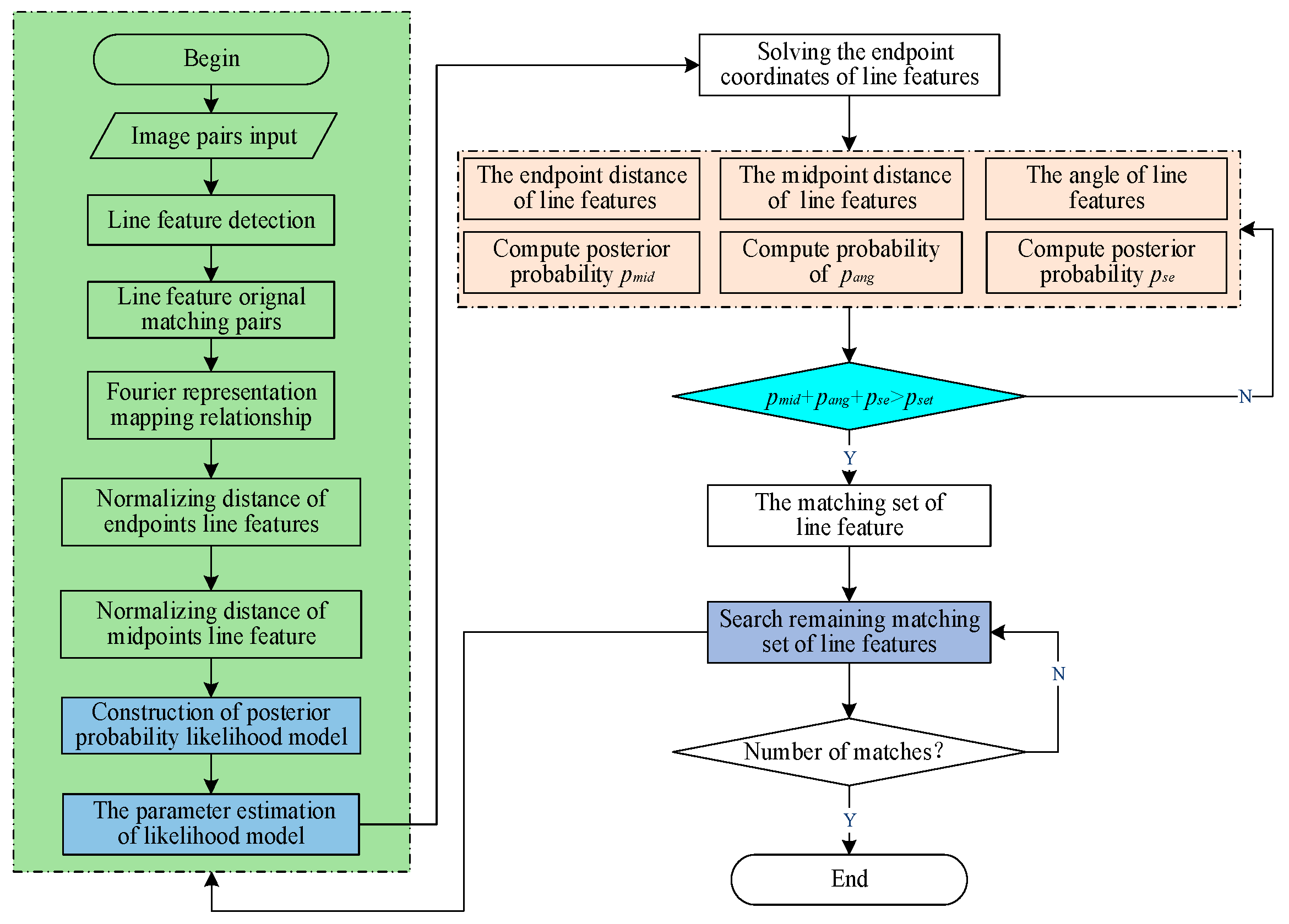
Figure 1. The flow chart of line feature matching algorithm proposed in this paper.
Electronics 14 03783 g001
Figure 2. Schematic illustration of geometric constraints for line feature matching.
Electronics 14 03783 g002
Figure 3. Schematic illustration of midpoint, endpoint distance and angle constraints derived from line feature pairs. (a) The endpoint and angle constraints (satisfying Conditions A and C, not satisfying Condition B); (b) the endpoint and midpoint constraints (satisfying conditions A and B, not satisfying C).
Electronics 14 03783 g003
Figure 6. Variation in the number of line feature matches with different λ and γ.
Electronics 14 03783 g006
Figure 12. From 2D line feature matching to 3D reconstruction.
Electronics 14 03783 g012
Figure 13. Comparison of time efficiency among the four matching algorithms (unit: seconds).
Electronics 14 03783 g013
Figure 4. The image pairs from different scenarios or cases are used to validate and evaluate the line feature matching algorithm proposed in this paper [52,53]. (a): Rotation; (b): view changing; (c,d): weak texture; (f): illumination variation; (e,g): low texture; (h): rotation + low texture.
Electronics 14 03783 g004
Figure 7. Comparison of matching results across the four algorithms for image pairs (c), (d), and (e).
Electronics 14 03783 g007
Figure 8. The ablation study comparison under three constraint conditions.
Electronics 14 03783 g008
Figure 9. The ablation study of line-matching performance under three constraint conditions.
Electronics 14 03783 g009
Figure 10. The line feature matching results comparison: Our Method versus LineTR, SOLD2, and WLD.
Electronics 14 03783 g010
Figure 11. Examples of image pairs (af) under different lighting conditions selected for the experiment.
Electronics 14 03783 g011
Table 1. A quantitative comparison of the matching results between our method and those of Refs. [32,35,40].
“Point + Line” InvariantLine Junction Line (LJL)Hybrid MatchingOur Method
(I1-line, I2-line)/MMC/MP(I1-line, I2-line)/MMC/MP(I1-line, I2-line)/MMC/MP(I1-line, I2-line)/MMC/MP
(a)[210, 213]/166166/1.0[218, 214]/167167/1.0—/——/—[210, 213]/127125/0.98
(b)[291, 291]/0—/—[481, 421]/337337/1.0—/——/—[485, 429]/362362/1.0
(c)[70, 63]/4747/1.0[69, 61]/3838/1.0[70, 63]/4744/1.0[70, 63]/5252/1.0
(d)[34, 34]/1616/1.0[35, 27]/1212/1.0[34, 34]/2121/1.0[34, 34]/2525/1.0
(e)[139, 113]/92—/—[24, 27]/1616/1.0[23, 24]/1717/1.0[23, 24]/1919/1.0
(f)[196, 59]/4545/1.0[196, 59]/2424/1.0[196, 59]/3630/0.83[196, 59]/3437/1.0
(g)[37, 36]/66/1.0[40, 38]/1717/1.0[37, 36]/1916/0.84[37, 36]/2120/0.95
(h)[139, 113]/9292/1.0[136, 119]/8989/1.0[139, 113]/7575/1.0[139, 113]/8484/1.0
Table 2. The comparative verification of the ablation experiments of our algorithm.
Condition A: (MC/M/MP)Condition A + B: (MC/M/MP)Condition A + B + C: (MC/M/MP)
(c)52/53/0.9852/52/1.052/52/1.0
(d)25/27/0.9325/26/0.9625/25/1.0
(h)82/92/0.8984/85/0.9984/84/1.0
Table 3. A quantitative comparison of line feature matching performance: LineTR, WLD, SOLD2, and Our Method.
LineTR (LSD)SOLD2WLD (LSD)Our Method (LSD)
M/MC/MPM/MC/MPM/MC/MPM/MC/MP
(a)156/144/0.92245/—/×253/—/×256/255/0.99
(b)368/364/0.99212/—/×413/—/×681/681/1.0
(c)172/170/0.98281/279/0.99113/107/0.95189/189/1.0
(d)54/54/1.066/64/0.9754/48/0.8968/67/0.99
(e)38/38/1.072/72/1.044/30/0.6871/71/1.0
(f)153/151/0.99245/243/0.99231/—/×130/129/0.99
(g)18/18/1.048/36/0.7557/—/×37/34/0.92
(h)78/73/0.94324/310/0.96216/—/×278/278/1.0
The bold indicates the optimal result.
Table 4. Comparison of experimental results of line feature-matching algorithms.
LBDfloat + FLANNLBDbinary + FLANNIILB + FLANNOur Method
(I1-line, I2-line)/MMC/MP(I1-line, I2-line)/MMC/MP(I1-line, I2-line)/MMC/MP(I1-line, I2-line)/MMC/MP
(a)[220, 213]/6363/1.0[220, 213]/114108/0.95[220, 213]/3735/0.94[220, 214]/126126/1.0
(b)[380, 380]/00/0.0[380, 380]/304298/0.98[380, 380]/50/0.0[380, 380]/307307/1.0
(c)[70, 63]/5151/1.0[70, 63]/4646/1.0[70, 63]/3939/1.0[70, 63]/5252/1.0
(d)[34, 34]/2525/1.0[34, 34]/2222/1.0[34, 34]/1717/1.0[34, 34]/2525/1.0
(e)[23, 24]/2121/1.0[23, 24]/1818/1.0[23, 24]/1111/1.0[23, 24]/1919/1.0
(f)[35, 34]/00/0[35, 34]/107/0.7[35, 34]/00/0[35, 34]/1312/0.92
(g)[37, 36]/1413/0.93[37, 36]/1615/0.94[37, 36]/109/0.9[37, 36]/1918/0.95
(h)[139, 113]/3232/1.0[139, 113]/5653/0.95[139, 113]/2221/0.95[139, 113]/8484/1.0
The bold indicates the optimal result.
Table 5. A quantitative comparison of matching performance between the method of [34] and Our method.
IILB + FLANNOur Method
The Total Number of Line
/The Total Matches (M)
MC/MPThe Total Number of Line
/The Total Matches (M)
MC/MP
(a–b)[291, 250]/17580/0.46[337, 304]/220220/1.0
(a–c)[291, 224]/14559/0.41[337, 279]/199199/1.0
(a–d)[291, 210]/13828/0.20[337, 244]/151151/1.0
(a–e)[291, 177]/14437/0.26[337, 222]/134134/1.0
(a–f)[291, 174]/12114/0.12[337, 189]/9292/1.0
The bold indicates the optimal result.
Disclaimer/Publisher’s Note: The statements, opinions and data contained in all publications are solely those of the individual author(s) and contributor(s) and not of MDPI and/or the editor(s). MDPI and/or the editor(s) disclaim responsibility for any injury to people or property resulting from any ideas, methods, instructions or products referred to in the content.