Multi-Sensor Fractional Order Information Fusion Suboptimal Filter with Time Delay

Abstract

A distributed weighted fusion fractional order filter is proposed for multi-sensor multi-delay fractional order systems. Firstly, the time-delay system is transformed into a non-time-delay system using the state augmentation method, and the optimal augmented fractional Kalman filter is derived. Secondly, in order to reduce the computational burden, a suboptimal fractional order Kalman filter is presented. Compared with the optimal augmented method, it greatly reduces the computational complexity, which is convenient for real-time applications. Then, in order to derive the weighting coefficient for distributed fusion, the calculation formula of filtering error variance matrix between any two sensor subsystems is derived. Finally, the distributed weighted fusion fractional order filter is presented. It is local optimal and globally suboptimal: compared with each local filter, it has higher accuracy; compared with the centralized fusion filter, it has lower accuracy and more fault tolerance. In summary, it is more suitable for practical application. Simulation results verify the effectiveness of the proposed algorithm.

1. Introduction

Fractional calculus stems from the promotion of the concept of integer calculus. The exploration and research of fractional calculus have a history spanning over 300 years. Fractional calculus is capable of describing materials and processing with memory and genetic properties, and is extensively applied in diverse domains of life, such as anomalous diffusion phenomena in environmental and engineering fields [1,2], fractional viscoelastic theory in physics [3,4], etc.

The Kalman filter represents a robust state observer capable of acquiring effective state information in the presence of environmental noise. Presently, based on the classical Kalman filter, multitude of extended studies have been carried out encompassing the extended Kalman filter [5], adaptive Kalman filter [6], the traceless Kalman filter [7], and others. With the advent of fractional order dynamic models, fractional order Kalman filter is commonly employed to address state estimation issues in fractional order systems. A fractional order operator discretization method based on G-L difference was put forward in [8,9]. A discretization method based on the Tustin generation function and the Al Alaoui operator was proposed in [10]. In order to solve linear and nonlinear fractional order state estimation problems, the fractional order extended Kalman filters were presented in [11,12]. Furthermore, the fractional order filter to tackle the problem of state estimation with correlated fractional order colored process noise was proposed in [13]. However, the above references all do not take into account the time-delay problem of fractional order systems.

In fact, the existence of a time delay is inescapable in practical applications. Regarding the state estimation of integer order systems with time delays, the state augmentation method is utilized to equivalently transform the time-delay system into an augmented system without time delay [14,15], and the state estimation was subsequently conducted. Nevertheless, The drawback of augmentation method is that high-dimensional state augmentation, which is not applicable to practical applications. To circumvent dimensionality increase, the estimation of time-delay systems is directly based on the minimum variance theory and the projection theorem in [16]. However, the complex multi-step smoother operations are requisite in time-delay filtering algorithms. The delayed observation sequences were transformed into normal system observation sequences in [17]. Though the recombination of observation sequences with time delays, an optimization algorithm for calculating the Kalman filter of time-delay systems was proposed [17]. By recombining the innovation sequence, the delay phenomenon in the system is eliminated, and the state estimation is realized. Currently, there is relatively limited research on state estimation for delay fractional order systems. A filtering algorithm for delay fractional order systems was investigated in [18], which effectively resolved the delay phenomenon in fractional order systems by integrating model transformation with a fractional order smoother. The integer order recombination innovation method was extended to fractional order systems, and the state estimation of the system was obtained via the recombination innovation sequence method in [19]. Nevertheless, the above references have not taken into account the distributed fusion problem of multi-sensor fractional order systems [20,21]. The image fusion algorithms for the fractional order system were proposed in [20,21]. But the time-delay situation has not been taken into account. The derivation of state estimation for multi-sensor time-delay fractional order systems is currently intricate

In this paper, the time-delay fractional order system subsequent to G-L discretization is investigated. Firstly, a delay fractional order filter based on the state augmentation method is proposed, which has no accuracy loss during model transformation. In order to mitigate the computational complexity, a suboptimal delay fractional order filter is presented in this paper. This filter not only circumvents the dimensionality increase induced by state augmentation method, but also avoids the intricate multi-step smoothing calculation in delay fractional order filtering [16]. Finally, the cross-covariance matrix between any two local subsystems is derived, and a distributed fusion filter based on local suboptimal delay fractional order filters is proposed.

The contributions of this paper are given as follows:

• Based on G-L discretization, the linear continuous fractional order systems with time delay were converted to the linear discrete fractional order systems. It solved the model conversion problem of fractional order systems with time delay.
• Based on the state augmentation method, a delay fractional order filter is proposed. It solved state estimation problem of time-delay fractional order system.
• By substituting smoothing with filtering approximation, a suboptimal time-delay fractional order filter is derived. It greatly reduces the computational burden.
• In order to compute the distributed fusion filter coefficient, the cross-covariance matrix between any two local subsystems is derived. It solved the problem of calculating the inter-covariance of local estimation errors.
• A distributed fusion filter is proposed based on local time-delay fractional order filters. It solved the fusion estimation problem of multi-sensor time-delay fractional order system.

2. Problem Formulation

Currently, there are three definition forms of fractional operators: Grünwald-Letnikov (G-L) definition, Caputo definition and Riemann Liouville (R-L) definition [22,23]. The G-L definition is derived from the difference approximation of integer order differential, and the definition of integer order differential is extended to the definition of fractional order. This definition is more appropriate for the application in signal processing. In this paper, the G-L fractional calculus definition is employed to discrete the fractional order system

The G-L difference of order of function is defined as [18]

$${\Delta }^{\alpha }{x}_k={\displaystyle \frac{1}{T^{\alpha }}}{{\sum }_{m=0}^k(-1)}^m\left(\begin{array}{c}\alpha \\ m\end{array}\right)x_{k-m}$$

(1)

where ${\Delta }^{\alpha }$ is a differential operator of order $\alpha$, $T$ is the sampling period, and $\left(\begin{array}{c}\alpha \\ m\end{array}\right)$ is calculated as follows:

$$\left(\begin{array}{c}\alpha \\ m\end{array}\right)=\left\{\begin{array}{c}1\hspace{1em}\hspace{1em}\hspace{1em}\hspace{1em}\hspace{1em}\hspace{1em}\hspace{1em}\hspace{1em}\hspace{1em}\hspace{1em} m=0\hfill \\ {\displaystyle \frac{\alpha (\alpha -1)\cdots (\alpha -m+1)}{m!}}\begin{array}{cc}& m>0\end{array}\hfill \end{array}\right.$$

(2)

when $m>k, x_{k-m}=0$. The approximate expression of the order differential operator $\alpha$ based on the G-L difference is

$${{}_0{}^{GL}D}_t^{\alpha }{x}_t\approx {\Delta }^{\alpha }{x}_k={\displaystyle \frac{1}{T^{\alpha }}}{{\sum }_{m=0}^k(-1)}^m\left(\begin{array}{c}\alpha \\ m\end{array}\right)x_{k-m}$$

(3)

where ${{}_0{}^{GL}D}_t^{\alpha }$ represents $\alpha$ order fractional differential operator from 0 to t, $\alpha$ represents the order of the fractional operation.

Taking the sampling time $T=1$, we can obtain

$${\Delta }^{\alpha }{x}_k={{\sum }_{m=0}^k(-1)}^m\left(\begin{array}{c}\alpha \\ m\end{array}\right)x_{k-m}$$

(4)

where $\alpha$ is the order of the fractional order, and the value is any real number. At that time $\alpha =0$, both sides of the equation are $x_k$, and

$$\begin{array}{l}{\Delta }^1{x}_{k+1}=x_{k+1}-x_k\\ {\Delta }^2{x}_{k+1}=x_{k+1}-2x_k-x_{k-1}\end{array}$$

(5)

Considering the state-space expression of a traditional discrete linear integer system, it can be seen that the state space expression of the one order linear discrete fractional system with multi-time delay is

$$\begin{array}{l}{\Delta }^1{x}_{k+1}={A_{\alpha }x}_k+B{u}_k+w_k\\ x_{k+1}={\Delta }^1{x}_{k+1}+x_k\\ y_k^{\left(i\right)}={\sum }_{n=0}^{d_i}{C}_n^{\left(i\right)}{x}_{k-n}+v_k^{\left(i\right)}\end{array}$$

(6)

where $A_{\alpha }=A-I$, $I$ is the unit matrix. $x_k\in {\mathbb{R}}^n$ is the state, $y_k^{\left(i\right)}\in {\mathbb{R}}^m$ is the measurement, $u_k\in {\mathbb{R}}^p$ is a known control input, $w_k\in {\mathbb{R}}^n$ and $v_k^{\left(i\right)}\in {\mathbb{R}}^m$ are Gaussian white noises with zero means and variance matrices Q and $R_i$. Superscript (i) denotes the ith sensor, $L$ is the number of sensors, and time-delay $d_i$ is the measurement delay of the ith sensor, with $0\le d_i\le d$, where d is a fixed positive integer.

Expanding the order $\alpha$ to any order, the multi-sensor state space expression of the linear discrete fractional order with multi-time delay is derived as

$$x_{k+1}=A_a{x}_k+B{u}_k+w_k-{\sum }_{m=1}^{k+1}(-1{)}^m{r}_m{x}_{k+1-m}$$

(7)

$$y_k^{\left(i\right)}={\sum }_{n=0}^{d_i}{C}_n^{\left(i\right)}{x}_{k-n}+v_k^{\left(i\right)}$$

(8)

where $r_m=\mathrm{diag}\left[\left(\begin{array}{c}{\alpha }_1\\ m\end{array}\right)\cdots \left(\begin{array}{c}{\alpha }_N\\ m\end{array}\right)\right],{\alpha }_1, \cdots {\alpha }_N$ are the orders of system equations and $N$ is the number of these equations.

Assumption 1.

$w_k$ and $v_k^{\left(i\right)}, i=1, 2, \cdots , L$ are independent white noises with zero mean, and the variances $Q>0$ and $R_i>0$.

Assumption 2.

The Initial state $x_k, k=0,-1, \cdots ,-d$ is independent of $w_k$ and $v_k^{\left(i\right)}, i=1, 2, \cdots , L$, and satisfies

$$E\left[x_k\right]={\mu }_k$$

(9)

$$E\left[\right(x_k-{\mu }_k\left)\right(x_k-{\mu }_k{)}^T]=P_k$$

(10)

Assumption 3.

Filtering errors  ${\tilde{x}}_{k|k}^{\left(i\right)}$ and ${\tilde{x}}_{k|k}^{\left(j\right)}, i\ne j$ are uncorrelated, where ${\tilde{x}}_{k|k}^{\left(i\right)}=x_{k|k}-{\widehat{x}}_{k|k}^{\left(i\right)}$, and ${\widehat{x}}_{k|k}^{\left(i\right)}$ is the filter based on the ith sensor subsystem.

Based on the observation $\left({y_1}^{\left(i\right)}, \cdots , {y_k}^{\left(i\right)}\right), i=1,2,\cdots ,L$, the linear minimum variance estimation ${\widehat{x}}_{k|k}^{\left(i\right)}$ of local sensor state $x_k^{\left(i\right)}$ will be given using augmented and non-augmented methods, respectively. Moreover, the distributed weighted fusion filter ${\widehat{x}}_{k|k}^{\left(m\right)}$ is also presented based on local estimation error covariance matrices${ P}_{k+1|k}^{\left(ij\right)}, i, j=1,2,\cdots ,L$.

3. Single Sensor Fractional Kalman Filter with Time Delay

3.1. State Augmentation Method

For time-delay fractional order systems Equations (7) and (8), expanding state $X_k$ to

$$X_k=[\begin{array}{cc}{x}_k^T& x_{k-1}^T\cdots x_{k-d}^T\end{array}{]}^T$$

(11)

Define${\underline{ A}}_a,{\underline{r}}_m,\underline{B}$ and ${\underline{C}}^{\left(i\right)}$ as

$${\underline{A}}_a={\left[\begin{array}{ccccc}{A}_a& 0& 0& \cdots & 0\\ I_n& 0& 0& \cdots & 0\\ 0& I_n& 0& \cdots & 0\\ ⋮& ⋮& ⋮& \ddots & ⋮\\ 0& \cdots & 0& I_n& 0\end{array}\right]}_{(d_i+1)n\times (d_i+1)n}, {\underline{r}}_m={\left[\begin{array}{ccccc}{r}_m& 0& 0& \cdots & 0\\ 0& 0& 0& \cdots & 0\\ 0& 0& 0& \cdots & 0\\ ⋮& ⋮& ⋮& \ddots & ⋮\\ 0& \cdots & 0& 0& 0\end{array}\right]}_{(d_i+1)n\times (d_i+1)n}$$

(12)

$${\underline{B}}_a={\left[\begin{array}{ccccc}{B}_a^T& 0& 0& \cdots & 0\end{array}\right]}_{(d_i+1)n\times 1}^T$$

(13)

$${\underline{C}}^{\left(i\right)}=[\begin{array}{ccccc}{C}_1^{\left(i\right)}& C_2^{\left(i\right)}& \cdots & C_{d_i-1}^{\left(i\right)}& C_{d_i}^{\left(i\right)}\end{array}{]}_{1\times (d_i+1)n}$$

(14)

where $n$ is the dimension, $d_i$ is the number of delay steps, $i=1\cdots L$.

So the equivalent augmented models of delay fractional order systems Equations (7) and (8) are

$$X_{k+1}={\underline{A}}_a{X}_k+\underline{B}{u}_k-{{\sum }_{m=1}^{k+1}(-1)}^m{\underline{r}}_m{X}_{k+1-m}+w_k$$

(15)

$$y_k^{\left(i\right)}={\underline{C}}^{\left(i\right)}{X}_k+v_k^{\left(i\right)}$$

(16)

For augmented systems Equations (15) and (16), using the G-L fractional order Kalman filtering method, we can obtain a delayed fractional order Kalman filter ${\widehat{X}}_{k|k}^{\left(i\right)}$ based on the state augmentation method.

Theorem 1.

In the case of Assumptions 1–3, augmented fractional order systems Equations (15) and (16) have local filters

$${\widehat{X}}_{k+1|k+1}^{\left(i\right)}={\widehat{X}}_{k+1|k}^{\left(i\right)}+K_{k+1}^{\left(i\right)}{\epsilon }_{k+1}^{\left(i\right)}$$

(17)

$${\epsilon }_{k+1}^{\left(i\right)}=y_{k+1}^{\left(i\right)}-{\underline{C}}^{\left(i\right)}{\widehat{X}}_{k+1|k}^{\left(i\right)}$$

(18)

$${\widehat{X}}_{k+1|k}^{\left(i\right)}={\underline{A}}_a{\widehat{X}}_{k|k}^{\left(i\right)}+{\underline{B}}_a{u}_k-{{\sum }_{m=1}^{k+1}(-1)}^m{\underline{r}}_m{\widehat{X}}_{k+1-m|k}^{\left(i\right)}$$

(19)

$$K_{k+1}^{\left(i\right)}=P_{k+1|k}^{\left(i\right)}{{\underline{C}}^{\left(i\right)}}^T[{\underline{C}}^{\left(i\right)}{P}_{k+1|k}^{\left(i\right)}{{\underline{C}}^{\left(i\right)}}^T+R_i{]}^{-1}$$

(20)

$$P_{k+1|k}^{\left(i\right)}=({\underline{A}}_a+{\underline{r}}_1)P_{k|k}^{\left(i\right)}({\underline{A}}_a+{\underline{r}}_1{)}^T+{\sum }_{m=2}^k{\underline{r}}_m{P}_{k-m|k-m}^{\left(i\right)}{\underline{r}}_m^T+Q$$

(21)

$$P_{k+1|k+1}^{\left(i\right)}=[I_n-K_{k+1}^{\left(i\right)}{\underline{C}}^{\left(i\right)}]P_{k+1|k}^{\left(i\right)}$$

(22)

Furthermore, the local time-delay fractional order Kalman filter ${\widehat{\mathrm{x}}}_{\mathrm{k}|\mathrm{k}}^{\left(\mathrm{i}\right)}$ of the original delay fractional order system can be obtained as

$${\widehat{x}}_{k|k}^{\left(i\right)}=\left[\begin{array}{cccc}{I}_n& 0& \cdots & 0\end{array}\right]{\widehat{X}}_{k|k}^{\left(i\right)}$$

(23)

Proof. 

The miniaturization performance index of the $i$-th sensor is

$$J=E\left[\right(X_k-{\widehat{X}}_{k|k}^{\left(i\right)}{)}^T(X_k-{\widehat{X}}_{k|k}^{\left(i\right)})]$$

(24)

In the case of minimization performance indicators, the problem of filtering lies in the projection [9]

$${\widehat{X}}_{k|k}^{\left(i\right)}=\mathrm{proj}(X_k|y_1^{\left(i\right)},\cdots ,y_k^{\left(i\right)})$$

(25)

According to the recursive projection equation [9], the recursive relation can be obtained as Equation (17) and

$$K_{k+1}^{\left(i\right)}=E\left[X_{k+1}^{\left(i\right)}{\epsilon }_{k+1}^{\left(i\right)T}\right]\left\{E\right[{\epsilon }_{k+1}^{\left(i\right)}{\epsilon }_{k+1}^{\left(i\right)T}]{\}}^{-1}$$

(26)

with $K_{k+1}^{\left(i\right)}$ called Kalman filter gain. For Equation (7), both sides of the equation are taken projections at the same time, it follows that

$$\begin{gathered} {\widehat{X}}_{k+1|k}^{\left(i\right)}={\underline{A}}_a{\widehat{X}}_{k|k}^{\left(i\right)}+\underline{B}{u}_k-\mathrm{proj}({\sum }_{m=1}^{k+1}(-1{)}^m{\underline{r}}_m{X}_{k+1-m}|y_1^{\left(i\right)},\cdots ,y_k^{\left(i\right)})+ \\ \mathrm{proj}(w_k|y_1^{\left(i\right)},\cdots ,y_k^{\left(i\right)}) \end{gathered}$$

(27)

Iterating the state Equation (7) yields

$${\widehat{X}}_{k|k}^{\left(i\right)}\in L(w_{k-1},\cdots ,w_0,X_0)$$

(28)

Applying the measurement Equation (8), we have

$$y_k^{\left(i\right)}\in L(v_k^{\left(i\right)},w_{k-1},\cdots ,w_0,X_0)$$

(29)

So we can obtain

$$L\left(y_1^{\left(i\right)}, \cdots , y_k^{\left(i\right)}\right)\subset L(v_k^{\left(i\right)}, \cdots , v_1^{\left(i\right)}, w_{k-1}, \cdots , w_0, X_0)$$

(30)

From Equation (30) and Assumptions 1–3, we have

$$w_k\perp L(y_1^{\left(i\right)}, \cdots , y_k^{\left(i\right)})$$

(31)

$$v_{k+1}^{\left(i\right)}\perp L(y_1^{\left(i\right)}, \cdots , y_k^{\left(i\right)})$$

(32)

Applying the projection formula Equation (30) and $E\left(w_k\right)=0$ yields

$$\mathrm{proj}(w_k\perp y_1^{\left(i\right)}, \cdots , y_k^{\left(i\right)})=0$$

(33)

$$\mathrm{proj}(v_{k+1}^{\left(i\right)}\perp y_1^{\left(i\right)}, \cdots , y_k^{\left(i\right)})=0$$

(34)

So Equation (28) is

$${\widehat{X}}_{k+1|k}^{\left(i\right)}={\underline{A}}_a{\widehat{X}}_{k|k}^{\left(i\right)}+\underline{B}{u}_k-\mathrm{proj}\left({\sum }_{m=1}^{k+1}(-1{)}^m{\underline{r}}_m{X}_{k+1-m}|y_1^{\left(i\right)}, \cdots , y_k^{\left(i\right)}\right)$$

(35)

For the last term of the above equation, we can use the following simplified hypothesis [9]

$$\begin{array}{l}\mathrm{proj}({\displaystyle \sum _{m=1}^{k+1}}(-1{)}^m{\underline{r}}_m{X}_{k+1-m}|y_1^{\left(i\right)},\cdots ,y_k^{\left(i\right)})\cong \\ \hspace{1em}\mathrm{proj}({\sum }_{m=1}^{k+1}(-1{)}^m{\underline{r}}_m{X}_{k+1-m}|y_1^{\left(i\right)},\cdots ,y_{k+1-m}^{\left(i\right)})\end{array}$$

(36)

Among them $\mathrm{m}=1,\cdots ,\mathrm{k}+1$, this simplification implies that some measurements are abandoned, and the approximation of the one-step state prediction Equation (19) is obtained.

Taking the radiogram for the measurement Equation (8) and applying Equation (34), we have

$${\widehat{y}}_{k+1|k}^{\left(i\right)}={\underline{C}}^{\left(i\right)}{\widehat{X}}_{k+1|k}^{\left(i\right)}$$

(37)

Take the innovation expression as

$${\epsilon }_{k+1}^{\left(i\right)}=y_{k+1}^{\left(i\right)}-{\widehat{y}}_{k+1|k}^{\left(i\right)}=y_{k+1}^{\left(i\right)}-{\underline{C}}^{\left(i\right)}{\widehat{X}}_{k+1|k}^{\left(i\right)}$$

(38)

Applying Assumption 3, the filtering and prediction estimation errors are

$${\tilde{X}}_{k|k}^{\left(i\right)}=X_k-{\widehat{X}}_{k|k}^{\left(i\right)}$$

(39)

$${\tilde{X}}_{k+1|k}^{\left(i\right)}=X_{k+1}-{\widehat{X}}_{k+1|k}^{\left(i\right)}$$

(40)

The filtering and prediction estimation error variance matrices are denoted as

$$P_{k|k}^{\left(i\right)}=E\left[{\tilde{X}}_{k|k}^{\left(i\right)}{\tilde{X}}_{k|k}^{\left(i\right)T}\right]$$

(41)

$$P_{k+1|k}^{\left(i\right)}=E\left[{\tilde{X}}_{k+1|k}^{\left(i\right)}{\tilde{X}}_{k+1|k}^{\left(i\right)T}\right]$$

(42)

Applying the measurement Equation (8) and innovation Equation (38), we have

$${\epsilon }_{k+1}^{\left(i\right)}={\underline{C}}^{\left(i\right)}{\tilde{X}}_{k+1|k}^{\left(i\right)}+v_{k+1}^{\left(i\right)}$$

(43)

From the state Equations (7) and (19), we can obtain the prediction error

$${\tilde{X}}_{k+1|k}^{\left(i\right)}={\underline{A}}_a{\tilde{X}}_{k|k}^{\left(i\right)}-{\sum }_{m=1}^{k+1}(-1{)}^m{\underline{r}}_m{\tilde{X}}_{k+1-m|k+1-m}^{\left(i\right)}+w_k$$

(44)

According to Equation (17), we have the filtering error

$${\tilde{X}}_{k+1|k+1}^{\left(i\right)}={\tilde{X}}_{k+1|k}^{\left(i\right)}+K_{k+1}^{\left(i\right)}{\epsilon }_{k+1}^{\left(i\right)}$$

(45)

Substituting Equation (43) into Equation (45), it follows that

$${\tilde{X}}_{k+1|k+1}^{\left(i\right)}=\left[I_n-K_{k+1}^{\left(i\right)}{\underline{C}}^{\left(i\right)}\right]{\tilde{X}}_{k+1|k}^{\left(i\right)}-K_{k+1}^{\left(i\right)}{v}_{k+1}^{\left(i\right)}$$

(46)

and because

$${\tilde{X}}_{k|k}^{\left(i\right)}\in L(v_k^{\left(i\right)},\cdots ,v_1^{\left(i\right)},w_{k-1},\cdots ,w_0,X_0)$$

(47)

which yields

$$w_k\perp {\tilde{X}}_{k|k}^{\left(i\right)}$$

(48)

From Equation (48), we know that

$$E\left[w_k{\tilde{X}}_{k|k}^{\left(i\right)T}\right]=0$$

(49)

Substituting Equations (44) and (49) into Equation (42) yields the prediction error variance matrix Equation (21). Because of

$${\tilde{X}}_{k+1|k}^{\left(i\right)}\in L(v_k^{\left(i\right)},\cdots ,v_1^{\left(i\right)},w_{k-1},\cdots ,w_0,X_0)$$

(50)

We can obtain

$$v_{k+1}^{\left(i\right)}\perp {\tilde{X}}_{k+1|k}^{\left(i\right)}$$

(51)

From Equation (51), we know that

$$E\left[v_{k+1}^{\left(i\right)}{\tilde{X}}_{k+1|k}^{\left(i\right)T}\right]=0$$

(52)

Substituting Equation (52) into Equation (43) yields the innovation variance matrix

$$E\left[{\epsilon }_{k+1}^{\left(i\right)}{\epsilon }_{k+1}^{\left(i\right)T}\right]={\underline{C}}^{\left(i\right)}{P}_{k+1|k}^{\left(i\right)}{\underline{C}}^{\left(i\right)T}+R^{\left(i\right)}$$

(53)

Substituting Equation (46) into Equation (41), we have the error variance matrix

$$P_{k+1|k+1}^{\left(i\right)}=[I_n-K_{k+1}^{\left(i\right)}{\underline{C}}^{\left(i\right)}]P_{k+1|k}^{\left(i\right)}[I_n-K_{k+1}^{\left(i\right)}{\underline{C}}^{\left(i\right)}{]}^T+K_{k+1}^{\left(i\right)}{R}^{\left(i\right)}{K}_{k+1}^{\left(i\right)T}$$

(54)

$$E\left[X_{k+1}{\epsilon }_{k+1}^{\left(i\right)T}\right]=E\left[\right({\widehat{X}}_{k+1|k}^{\left(i\right)}+{\tilde{X}}_{k+1|k}^{\left(i\right)})\hspace{1em}({\underline{C}}^{\left(i\right)}{\tilde{X}}_{k+1|k}^{\left(i\right)}+v_{k+1}^{\left(i\right)}{)}^T]$$

(55)

From orthographic projection, we have

$${\widehat{X}}_{k+1|k}^{\left(i\right)}\perp {\tilde{X}}_{k+1|k}^{\left(i\right)}, v_{k+1}^{\left(i\right)}\perp {\widehat{X}}_{k+1|k}^{\left(i\right)}, v_{k+1}^{\left(i\right)}\perp {\tilde{X}}_{k+1|k}^{\left(i\right)}$$

(56)

so that

$$E\left[X_{k+1}{\epsilon }_{k+1}^{\left(i\right)\mathrm{T}}\right]=P_{k+1|k}^{\left(i\right)}{\underline{C}}^{\left(i\right)\mathrm{T}}$$

(57)

Substituting Equations (54) and (57) into the filtering gain Equation (26), we have Equation (20). Substituting filtering gain Equation (20) into the error variance matrix Equation (54) and simplifying yield Equation (22). The proof is completed. □

3.2. Non-State Augmented Method

To circumvent the augmentation of state dimensionality and mitigate the computational complexity, in Section 3.2, a suboptimal local delay fractional order Kalman filter is proposed by substituting smoothing with filtering approximation during the calculation the estimated values of measurement predictions. The term “suboptimal” implies that the accuracy of the filter of Theorem 2 is lower than that of Theorem 1 based on augmentation state algorithm due to the loss of accuracy by substituting smoothing with filtering approximation. Of course, the filter of Theorem 2 has the advantage of less computational in comparison with that of Theorem 1 based on augmentation state algorithm.

Theorem 2.

In the case of Assumptions 1–3, multi-sensor fractional order systems with time-delay Equations (1) and (2) have local suboptimal filters

$${\widehat{x}}_{k+1|k+1}^{\left(i\right)}={\widehat{x}}_{k+1|k}^{\left(i\right)}+K_{k+1}^{\left(i\right)}{\epsilon }_{k+1}^{\left(i\right)}$$

(58)

$${\epsilon }_{k+1}^{\left(i\right)}=y_{k+1}^{\left(i\right)}-C_0^{\left(i\right)}{\widehat{x}}_{k+1|k}^{\left(i\right)}-{\sum }_{n=1}^d{C}_n^{\left(i\right)}{\widehat{x}}_{k+1-n|k+1-n}^{\left(i\right)}$$

(59)

$${\widehat{x}}_{k+1|k}^{\left(i\right)}=A{\widehat{x}}_{k|k}^{\left(i\right)}+B_a{u}_k-{{\sum }_{m=1}^{k+1}(-1)}^m{r}_m{\widehat{x}}_{k+1-m|k+1-m}^{\left(i\right)}$$

(60)

$$P_{k+1|k}^{\left(i\right)}=(A_a+r_1)P_{k|k}^{\left(i\right)}(A_a+r_1{)}^T+{\sum }_{m=2}^{k+1}{r}_m{P}_{k+1-m|k+1-m}^{\left(i\right)}{r}_m^T+Q$$

(61)

$$P_{k+1|k+1}^{\left(i\right)}=\left(I-K_{k+1}^{\left(i\right)}{C}_0^{\left(i\right)}\right)P_{k+1|k}^{\left(i\right)}-K_{k+1}^{\left(i\right)}\left[C_1^{\left(i\right)}{P}_{k|k}^{\left(i\right)}{A}_a^T-{\sum }_{n=1}^{d_i}(-1{)}^n{C}_n^{\left(i\right)}{P}_{k+1-n|k+1-n}^{\left(i\right)}{r}_n^T\right]$$

(62)

$$\begin{array}{cc}{K}_{k+1}^{\left(i\right)}=\hfill & \left[P_{k+1|k}^{\left(i\right)}{C}_0^{\left(i\right)T}+A_a{P}_{k|k}^{\left(i\right)}{C}_1^{\left(i\right)T}-{\displaystyle \sum _{n=1}^{d_i}}(-1{)}^n{r}_n{P}_{k+1-n|k+1-n}^{\left(i\right)}{C}_n^{\left(i\right)T}\right]\times \hfill \\ & {\left[\begin{array}{l}{C}_0^{\left(i\right)}{P}_{k+1|k}^{\left(i\right)}{C}_0^{\left(i\right)T}+{\sum }_{n=1}^{d_i}{C}_n^{\left(i\right)}{P}_{k+1-n|k+1-n}^{\left(i\right)}{C}_n^{\left(i\right)T}+R^{\left(i\right)}+\\ C_0^{\left(i\right)}{A}_a{P}_{k|k}^{\left(i\right)}{C}_1^{\left(i\right)T}-{\sum }_{n=1}^{d_i}(-1{)}^n{C}_0^{\left(i\right)}{r}_n{P}_{k+1-n|k+1-n}^{\left(i\right)}{C}_n^{\left(i\right)T}+\\ C_1^{\left(i\right)}{P}_{k|k}^{\left(i\right)}{A}_a^T{C}_0^{\left(i\right)T}-{\sum }_{n=1}^{d_i}(-1{)}^n{C}_n^{\left(i\right)}{P}_{k+1-n|k+1-n}^{\left(i\right)}{r}_n^T{C}_0^{\left(i\right)T}\end{array}\right]}^{-1}\hfill \end{array}$$

(63)

where ${\widehat{x}}_{k+1|k+1}^{\left(i\right)}$ and ${\widehat{x}}_{k+1|k}^{\left(i\right)}$ are filter and one-step predictor, $P_{k+1|k+1}^{\left(i\right)}$ and $P_{k+1|k}^{\left(i\right)}$ are filtering error variance matrix and prediction error variance matrix, $K_{k+1}^{\left(i\right)}$ is the filter gain.

Proof. 

The objective of the fractional Kalman filter is to obtain the linear minimum variance estimation of state based on observation $\left({y_1}^{\left(i\right)}, \cdots , {y_k}^{\left(i\right)}\right)$, the minimum performance index of sensor $i$ as

$$J=E\left[\right(x_k-{\widehat{x}}_{k|k}^{\left(i\right)}{)}^T(x_k-{\widehat{x}}_{k|k}^{\left(i\right)})]$$

(64)

Under the minimization of the performance index, the filtering problem is to find the projection [24]

$${\widehat{x}}_{k|k}^{\left(i\right)}=\mathrm{proj}(x_k|{y_1}^{\left(i\right)},\cdots ,{y_k}^{\left(i\right)})$$

(65)

According to the recursive projection formula, we have the recursive relationship [25,26]

$${\widehat{x}}_{k+1|k+1}^{\left(i\right)}={\widehat{x}}_{k+1|k}^{\left(i\right)}+K_{k+1}^{\left(i\right)}{\epsilon }_{k+1}^{\left(i\right)}$$

(66)

$${\epsilon }_{k+1}^{\left(i\right)}=y_{k+1}^{\left(i\right)}-{\widehat{y}}_{k+1|k}^{\left(i\right)}$$

(67)

with ${\epsilon }_{k+1}^{\left(i\right)}$ as the innovation process. Applying the projection theorem to Equation (7), the one-step predictor is

$$\begin{gathered} {\widehat{x}}_{k+1|k}^{\left(i\right)}=\mathrm{proj}(x_{k+1}|{y_1}^{\left(i\right)},\cdots ,{y_k}^{\left(i\right)}) \\ =\mathrm{proj}\left(A_a{x}_k+B_a{u}_k+w_k-{\sum }_{m=1}^{k+1}(-1{)}^m{r}_m{x}_{k+1-m}|{y_1}^{\left(i\right)},\cdots ,{y_k}^{\left(i\right)}\right) \\ =A_a{\widehat{x}}_{k|k}^{\left(i\right)}+B_a{u}_k-\mathrm{proj}\left({\sum }_{m=1}^{k+1}(-1{)}^m{r}_m{x}_{k+1-m}|{y_1}^{\left(i\right)},\cdots ,{y_k}^{\left(i\right)}\right) \end{gathered}$$

(68)

Using the simplifying assumption as follows

$$\begin{array}{l}\mathrm{proj}\left({\sum }_{m=1}^{k+1}(-1{)}^m{r}_m{x}_{k+1-m}|{y_1}^{\left(i\right)},\cdots ,{y_k}^{\left(i\right)}\right)\\ \hspace{1em}\cong \mathrm{proj}\left({\sum }_{m=1}^{k+1}(-1{)}^m{r}_m{x}_{k+1-m}|{y_1}^{\left(i\right)},\cdots ,y_{k+1-m}^{\left(i\right)}\right)\end{array}$$

(69)

For $m=1, \cdots , k+1$. This simplification means discarding some measurements. Consequently, we obtain a suboptimal solution for the fractional order Kalman filter. So, the one-step predicted state is obtained as

$${\widehat{x}}_{k+1|k}^{\left(i\right)}=A_a{\widehat{x}}_{k|k}^{\left(i\right)}+B_a{u}_k-{{\sum }_{m=1}^{k+1}(-1)}^m{r}_m{\widehat{x}}_{k+1-m|k+1-m}^{\left(i\right)}$$

(70)

From Assumption 3, we can obtain the estimated error of the prediction ${\tilde{x}}_{k+1|k}^{\left(i\right)}=x_{k+1|k}^{\left(i\right)}-{\widehat{x}}_{k+1|k}^{\left(i\right)}$. From Equations (7) and (70), we can obtain

$${\tilde{x}}_{k+1|k}^{\left(i\right)}=A_a{\tilde{x}}_{k|k}^{\left(i\right)}-{{\sum }_{m=1}^{k+1}(-1)}^m{r}_m{\tilde{x}}_{k+1-m|k+1-m}^{\left(i\right)}+w_k$$

(71)

From Assumption 2, we can obtain$P_{k+1|k}^{\left(i\right)}=E\left[{\tilde{x}}_{k+1|k}^{\left(i\right)}{\tilde{x}}_{k+1|k}^{\left(i\right)T}\right]$, and from Equation (71), we can obtain

$$P_{k+1|k}^{\left(i\right)}=(A_a+r_1)P_{k|k}^{\left(i\right)}(A_a+r_1{)}^T+{\sum }_{m=2}^{k+1}{r}_m{P}_{k+1-m|k+1-m}^{\left(i\right)}{r}_m^T+Q$$

(72)

Applying the projection theorem to Equation (8), the estimated value of the measurement prediction is

$${\widehat{y}}_{k+1|k}^{\left(i\right)}=C_0^{\left(i\right)}{\widehat{x}}_{k+1|k}^{\left(i\right)}+{\sum }_{n=1}^{d_i}{C}_n^{\left(i\right)}{\widehat{x}}_{k+1-n|k}^{\left(i\right)}$$

(73)

For the estimated values of measurement and prediction, similar approximate methods to state prediction are also used. By simplifying the following assumptions

$${\sum }_{n=1}^{d_i}{C}_n^{\left(i\right)}{\widehat{x}}_{k+1-n|k}^{\left(i\right)}\cong {\sum }_{n=1}^{d_i}{C}_n^{\left(i\right)}{\widehat{x}}_{k+1-n|k+1-n}^{\left(i\right)}$$

(74)

The estimated value of suboptimal measurement and prediction is

$${\widehat{y}}_{k+1|k}^{\left(i\right)}=C_0^{\left(i\right)}{\widehat{x}}_{k+1|k}^{\left(i\right)}+{\sum }_{n=1}^{d_i}{C}_n^{\left(i\right)}{\widehat{x}}_{k+1-n|k+1-n}^{\left(i\right)}$$

(75)

From ${\epsilon }_{k+1}^{\left(i\right)}=y_{k+1}^{\left(i\right)}-{\widehat{y}}_{k+1|k}^{\left(i\right)}$, substituting Equations (8) and (73) into Equation (67), we can obtain

$$\begin{gathered} {\epsilon }_{k+1}^{\left(i\right)}=C_0^{\left(i\right)}{A}_a{\tilde{x}}_{k|k}^{\left(i\right)}-C_0^{\left(i\right)}{{\sum }_{m=1}^{k+1}(-1)}^m{r}_m{\tilde{x}}_{k+1-m|k+1-m}^{\left(i\right)}+ \\ {C}_0^{\left(i\right)}w(k)+{\sum }_{n=1}^{d_i}{C}_n^{\left(i\right)}{\tilde{x}}_{k+1-n|k+1-n}^{\left(i\right)}+v_{k+1}^{\left(i\right)} \end{gathered}$$

(76)

Subtracting Equation (7) from Equation (65), it follows that

$${\tilde{x}}_{k+1|k+1}^{\left(i\right)}={\tilde{x}}_{k+1|k}^{\left(i\right)}-K_{k+1}^{\left(i\right)}{\epsilon }_{k+1}^{\left(i\right)}$$

(77)

Substituting Equations (71) and (76) into Equation (77), we have

$$\begin{gathered} {\tilde{x}}_{k+1|k+1}^{\left(i\right)}=\left(I-K_{k+1}^{\left(i\right)}{C}_0^{\left(i\right)}\right)\left[A_a{\tilde{x}}_{k|k}^{\left(i\right)}-{\sum _{m=1}^{k+1}(-1)}^m{r}_m{\tilde{x}}_{k+1-m|k+1-m}^{\left(i\right)}+w_k\right]- \\ {K}_{k+1}^{\left(i\right)}\left[{\sum }_{n=1}^{d_i}{C}_n^{\left(i\right)}{\tilde{x}}_{k+1-n|k+1-n}^{\left(i\right)}+v_{k+1}^{\left(i\right)}\right] \end{gathered}$$

(78)

Under Assumption 2, we can obtain $P_{k+1|k+1}^{\left(i\right)}=E\left[{\tilde{x}}_{k+1|k+1}^{\left(i\right)}{\tilde{x}}_{k+1|k+1}^{\left(i\right)T}\right]$. Considering ${\tilde{x}}_{k+1|k+1}^{\left(i\right)}\perp w_k$, ${\tilde{x}}_{k+1|k+1}^{\left(i\right)}\perp v_{k+1}^{\left(i\right)}$, we have

$$\begin{array}{l}{P}_{k+1|k+1}^{\left(i\right)}=\left(I-K_{k+1}^{\left(i\right)}{C}_0^{\left(i\right)}\right)P_{k+1|k}^{\left(i\right)}{\left(I-K_{k+1}^{\left(i\right)}{C}_0^{\left(i\right)}\right)}^T\\ \hspace{1em}\hspace{1em}\hspace{1em}\hspace{1em}\hspace{1em}\hspace{1em} +K_{k+1}^{\left(i\right)}\left[{\displaystyle \sum _{n=1}^{d_i}}{C}_n^{\left(i\right)}{P}_{k+1-n|k+1-n}^{\left(i\right)}{C}_n^{\left(i\right)T}+R^{\left(i\right)}\right]K_{k+1}^{\left(i\right)T}\\ \hspace{1em}\hspace{1em}\hspace{1em}\hspace{1em}\hspace{1em}\hspace{1em} -\left(I-K_{k+1}^{\left(i\right)}{C}_0^{\left(i\right)}\right)\left[A_a{P}_{k|k}^{\left(i\right)}{C}_1^{\left(i\right)T}-{\displaystyle \sum _{n=1}^{d_i}}(-1{)}^n{r}_n{P}_{k+1-n|k+1-n}^{\left(i\right)}{C}_n^{\left(i\right)T}\right]K_{k+1}^{\left(i\right)T}-\\ \hspace{1em}\hspace{1em}\hspace{1em}\hspace{1em}\hspace{1em} K_{k+1}^{\left(i\right)}\left[C_1^{\left(i\right)}{P}_{k|k}^{\left(i\right)}{A}_a^T-{\sum }_{n=1}^{d_i}(-1{)}^n{C}_n^{\left(i\right)}{P}_{k+1-n|k+1-n}^{\left(i\right)}{r}_n^T\right]{\left(I-K_{k+1}^{\left(i\right)}{C}_0^{\left(i\right)}\right)}^T\end{array}$$

(79)

To minimize the performance index $J$, the filter gain $K_{k+1}^{\left(i\right)}$ should be obtained by ${\displaystyle \frac{\partial tr{P}_{k+1}^{\left(i\right)}}{\partial K_{k+1}^{\left(i\right)}}}=0$. From the differential operation formula of matrix trace and Equation (79), we have a suboptimal filter gain

$$\begin{array}{ll}{K}_{k+1}^{\left(i\right)}=& \left[P_{k+1|k}^{\left(i\right)}{C}_0^{\left(i\right)T}+A_a{P}_{k|k}^{\left(i\right)}{C}_1^{\left(i\right)T}-{\displaystyle \sum _{n=1}^{d_i}}(-1{)}^n{r}_n{P}_{k+1-n|k+1-n}^{\left(i\right)}{C}_n^{\left(i\right)T}\right]\times \\ & {\left[\begin{array}{l}{C}_0^{\left(i\right)}{P}_{k+1|k}^{\left(i\right)}{C}_0^{\left(i\right)T}+{\sum }_{n=1}^{d_i}{C}_n^{\left(i\right)}{P}_{k+1-n|k+1-n}^{\left(i\right)}{C}_n^{\left(i\right)T}+R^{\left(i\right)}+\\ C_0^{\left(i\right)}{A}_a{P}_{k|k}^{\left(i\right)}{C}_1^{\left(i\right)T}-{\sum }_{n=1}^{d_i}(-1{)}^n{C}_0^{\left(i\right)}{r}_n{P}_{k+1-n|k+1-n}^{\left(i\right)}{C}_n^{\left(i\right)T}+\\ C_1^{\left(i\right)}{P}_{k|k}^{\left(i\right)}{A}_a^T{C}_0^{\left(i\right)T}-{\sum }_{n=1}^{d_i}(-1{)}^n{C}_n^{\left(i\right)}{P}_{k+1-n|k+1-n}^{\left(i\right)}{r}_n^T{C}_0^{\left(i\right)T}\end{array}\right]}^{-1}\end{array}$$

(80)

Substituting Equation (79) into Equation (80), we have

$$P_{k+1|k+1}^{\left(i\right)}=\left(I-K_{k+1}^{\left(i\right)}{C}_0^{\left(i\right)}\right)P_{k+1|k}^{\left(i\right)}-K_{k+1}^{\left(i\right)}\left[C_1^{\left(i\right)}{P}_{k|k}^{\left(i\right)}{A}_a^T-{\sum }_{n=1}^{d_i}(-1{)}^n{C}_n^{\left(i\right)}{P}_{k+1-n|k+1-n}^{\left(i\right)}{r}_n^T\right]$$

(81)

The proof is completed. □

4. Multi-Sensor Fractional Kalman Filter with Time Delay

Next, the calculation amount of each time using the augmented method and non-augmented method is given, and only multiplication and division methods with large calculation amounts are discussed here. When $n\times m$ matrix is multiplied by $m\times p$ matrix, there are $n\times m\times p$ multiplication operations at each time; Calculating the inverse of the $n\times n$ matrix, there are $n^3$ division operations at each time; It can be seen from the calculation that the multiplication and division operations at each time of the prediction error variance matrix Equation (21) of the augmented algorithm and the prediction error variance matrix Equation (66) of the non augmented algorithm as $2n^3$, $n$ is the dimension of the sensor.

It can be seen that, compared with the state augmentation method, the non-state augmentation method greatly reduces the real-time computation. In this section, based on the single sensor suboptimal fractional order Kalman filter, the cross-covariance matrix between any two local sensors in the multi-sensor system is derived. Furthermore, based on the distributed weighted fusion algorithm, the weighted fusion suboptimal fractional order filter is given.

Theorem 3.

Under Assumptions 1–3, there are suboptimal filtering and suboptimal error variance matrices between the $i$ th sensor and the $j$th sensor subsystem in the multi-time-delay fractional order system

$$P_{k+1|k}^{\left(ij\right)}=(A_a+r_1)P_{k|k}^{\left(ij\right)}(A_a+r_1{)}^T+{\sum }_{m=2}^k{r}_m{P}_{k-m|k-m}^{\left(ij\right)}{r}_m^T+Q$$

(82)

$$\begin{gathered} P_{k+1|k+1}^{\left(ij\right)}=\left(I-K_{k+1}^{\left(i\right)}{C}_0^{\left(i\right)}\right)P_{k+1|k}^{\left(ij\right)}{\left(I-K_{k+1}^{\left(j\right)}{C}_0^{\left(j\right)}\right)}^T \\ +K_{k+1}^{\left(i\right)}\left[{\sum }_{n=1}^{d_i}{C}_n^{\left(i\right)}{P}_{k+1-n|k+1-n}^{\left(ij\right)}{C}_n^{\left(j\right)T}\right]K_{k+1}^{\left(j\right)T} \\ -\left(I-K_{k+1}^{\left(i\right)}{C}_0^{\left(i\right)}\right)\left[A_a{P}_{k|k}^{\left(ij\right)}{C}_1^{\left(i\right)T}-{\sum }_{n=1}^{d_i}(-1{)}^n{r}_n{P}_{k+1-n|k+1-n}^{\left(ij\right)}{C}_n^{\left(j\right)T}\right]K_{k+1}^{\left(j\right)T} \\ -K_{k+1}^{\left(i\right)}\left[C_1^{\left(i\right)}{P}_{k|k}^{\left(ij\right)}{A}_a^T-{\sum }_{n=1}^{d_i}(-1{)}^n{C}_n^{\left(i\right)}{P}_{k+1-n|k+1-n}^{\left(ij\right)}{r}_n^T\right]{\left(I-K_{k+1}^{\left(j\right)}{C}_0^{\left(j\right)}\right)}^T \end{gathered}$$

(83)

Proof. 

Under Assumption 3 and Equation (76), we can obtain the suboptimal prediction error variance matrix of sensor $i$ and sensor $j$. Under Assumption 3 and Equation (83), we can obtain the suboptimal filtering error variance matrix of sensor $i$ and sensor $j$. The proof is completed. □

Theorem 4.

For system Equations (7) and (8) with Assumptions 1–3, we have the distributed weighted fusion filter

$${\widehat{x}}_{k|k}^{\left(m\right)}={\Omega }_{k|k}^{\left(1\right)}{\widehat{x}}_{k|k}^{\left(1\right)}+{\Omega }_{k|k}^{\left(2\right)}{\widehat{x}}_{k|k}^{\left(2\right)}+\cdots {\Omega }_{k|k}^{\left(L\right)}{\widehat{x}}_{k|k}^{\left(L\right)}$$

(84)

where ${\widehat{x}}_{k|k}^{\left(i\right)}, i=1, 2, \cdots , L$, are computed by Theorem 2. The fusion matrix weights ${\Omega }_{k|k}^{\left(i\right)}, i=1, 2, \cdots , L$ are computed by

$${\Omega }_{k|k}={\sum }_{k|k}^{-1}e(e^T{\sum }_{k|k}^{-1}e{)}^{-1}$$

(85)

where ${\sum }_{k|k}=\left(P_{k|k}^{\left(ij\right)}\right), i, j=1, 2, \cdots , l$ is an $nl\times nl$ symmetric positive definite matrix, where the filtering error covariance matrices $P_{k|k}^{\left(ij\right)}$ are computed by Theorems 2 and 3. ${\Omega }_{k|k}={\left[{\Omega }_{k|k}^{\left(1\right)}, {\Omega }_{k|k}^{\left(2\right)}, \cdots , {\Omega }_{k|k}^{\left(L\right)}\right]}^T$ and $e={\left[I_n, I_n, \cdots , I_n\right]}^T$ are both $nL\times n$ matrices. The corresponding variance of the weighted fusion suboptimal filter is computed by

$$P_{k|k}^{\left(m\right)}={\left(e^T{\sum }_{k|k}^{-1}e\right)}^{-1}$$

(86)

Proof. 

Based on the L unbiased estimates ${\widehat{x}}_{k|k}^{\left(i\right)}, i=1, 2, \cdots , L$, the problem is to obtain the unbiased fusion estimate ${\widehat{x}}_{k|k}^{\left(m\right)}$ given by Equation (85), i.e.,

$${\rm E}\left({\widehat{x}}_{k|k}^{\left(m\right)}\right)={\rm E}\left(x_k\right)$$

(87)

In the sense of linear minimum variance, the weighted matrices ${\Omega }_{k|k}^{\left(i\right)}, i=1,2,\cdots ,L$ should be chosen to minimize the sum $J$ of mean squares of components for the fusion estimation errors

$$J={\rm E}\left[{\tilde{x}}_{k|k}^{\left(m\right){\rm T}}{\tilde{x}}_{k|k}^{\left(m\right)}\right]\begin{array}{cc},& {\tilde{x}}_{k|k}^{\left(m\right)}=x_k-{\widehat{x}}_{k|k}^{\left(m\right)}\end{array}$$

(88)

It is equivalent to

$$J=\mathit{tr}{P}_{k|k}^{\left(m\right)}\begin{array}{cc},& P_{k|k}^{\left(m\right)}={\rm E}[{\tilde{x}}_{k|k}^{\left(m\right)}\end{array}{\tilde{x}}_{k|k}^{\left(m\right){\rm T}}]$$

(89)

The sign $tr$ indicates the trace of the matrix.

Applying the unbiasedness of the local and fusion estimations, from Equation (49), we have the constraint condition

$${\sum }_{i=1}^L{\Omega }_{k|k}^{\left(i\right)}=I_n$$

(90)

with $I_n$ as a $n\times n$ unit matrix. From the above equation, it follows that the fusion error expression Equation (85).

Introducing the $n\times nL$ composite undetermined matrix ${\Omega }_{k|k}$

$${\Omega }_{k|k}={\left[{\Omega }_{k|k}^{\left(1\right)},{\Omega }_{k|k}^{\left(2\right)},\cdots ,{\Omega }_{k|k}^{\left(L\right)}\right]}^T$$

(91)

Define $nL\times nL$ partitioned matrix $P$ with $e={\left[I_n, I_n, \cdots , I_n\right]}^T$ as the $(i, j)$ th element, i.e.,

$$P_{k|k}^{\left(m\right)}=\left[\begin{array}{ccc}{P}_{k|k}^{\left(1\right)}& 0& 0\\ 0& \ddots & 0\\ 0& 0& P_{k|k}^{\left(L\right)}\end{array}\right]$$

(92)

The performance indicators $J$ can be abbreviated as

$$J=\mathit{tr}{\Omega }_{k|k}{P}_{k|k}^{\left(m\right)}{\Omega }_{k|k}^{{\rm T}}$$

(93)

The constraint condition (95) can be written as

$${\Omega }_{k|k}e=I_n{\begin{array}{cc},& e=\left[\begin{array}{ccc}{I}_n& \cdots & I_n\end{array}\right]\end{array}}^{{\rm T}}$$

(94)

Therefore, the problem boils down to finding the matrix minimization performance index Equation (93) under the constraint condition Equation (94).

Because constraint Equation (94) is a matrix equation, it is equivalent to $n^2$ scalar constraint conditions by matrix elements. Apply the Lagrange multiplier method and introduce an auxiliary function

$$F=J+\mathit{tr}{\sum }_{i=1}^n{\lambda }_i({\Omega }_{k|k}e-I_n)e_i$$

(95)

where the row vector is defined

$${\lambda }_i={\left[{\lambda }_{i1},{\lambda }_{i2},\cdots ,{\lambda }_{in}\right]}^T\begin{array}{cc},& e_i^{{\rm T}}=[0\cdots 010\cdots 0]\end{array}$$

(96)

The element in the ith column of $e_i^{{\rm T}}$ is 1, and the remaining elements are zero.

The auxiliary function Equation (95) can be interpreted as: The matrix constraints ${\Omega }_{k|k}e=I_n$ are equivalent to $n^2$ scalar constraints by component, and $({\Omega }_{k|k}e-I_n)e_i$ is the $i$th column vector of matrix $({\Omega }_{k|k}e-I_n)$, ${\lambda }_i$ is the corresponding Lagrange multiplier row vector. The inner product ${\lambda }_i({\Omega }_{k|k}e-I_n)e_i$ of these two vectors is equivalent to introducing $n$ Lagrange multipliers with $n$ scalar constraints ${\lambda }_i={\left[{\lambda }_{i1}, {\lambda }_{i2}, \cdots , {\lambda }_{in}\right]}^T$. So the second term in Equation (95) introduces $n^2$ Lagrange multiplier corresponding to $n^2$ constraint conditions ${\lambda }_{ij},i, j=1, \cdots , n$.

Applying the matrix trace differential formula

$${\displaystyle \frac{\partial }{\partial X}}\mathit{tr}(XB{X}^{{\rm T}})=2XB(B=B^{{\rm T}})\begin{array}{cc},& {\displaystyle \frac{\partial }{\partial X}}\mathit{tr}(AXB)=A^{{\rm T}}{B}^{{\rm T}}\end{array}$$

(97)

Noting $P_{k|k}^{\left(m\right)}=P_{k|k}^{\left(m\right){\rm T}}$ and (60), and setting ${\displaystyle \frac{\partial F}{\partial A}}=0$, we have

$$2A{P}_{k|k}^{\left(m\right)}+{\sum }_{i=1}^n{\lambda }_i^{{\rm T}}(e{e}_i{)}^{{\rm T}}=0$$

(98)

The second item on the left side of the above equation is

$${\sum }_{i=1}^n{\lambda }_i^{{\rm T}}{e}_i^{{\rm T}}{e}^{{\rm T}}=[{\lambda }_1^{{\rm T}},\cdots ,{\lambda }_n^{{\rm T}}]\left[\begin{array}{c}{e}_1^{{\rm T}}\\ ⋮\\ e_n^{{\rm T}}\end{array}\right]e^{{\rm T}}={\Lambda }^{{\rm T}}{e}^{{\rm T}}$$

(99)

with the matrix $\Lambda$ defined as

$$\Lambda ={\left[{\lambda }_1, \cdots , {\lambda }_n\right]}^T=\left({\lambda }_{ij}\right)$$

(100)

Its $i$th row and $j$th column elements is${ \lambda }_{ij}$.

From the transposition of Equations (98) and (99), we have the relationship

$$P_{k|k}^{\left(m\right)}{\Omega }_{k|k}^{{\rm T}}+e{U}^{{\rm T}}=0$$

(101)

which is equivalent to

$$e^T{\Omega }_{k|k}^{{\rm T}}-I_n=0$$

(102)

Combining Equations (101) and (102) yields the matrix equation

$$\left[\begin{array}{cc}{P}_{k|k}^{\left(m\right)}& e\\ e^{{\rm T}}& 0\end{array}\right]\left[\begin{array}{c}{\Omega }_{k|k}^{\left(m\right){\rm T}}\\ U^{{\rm T}}\end{array}\right]=\left[\begin{array}{c}0\\ I_n\end{array}\right]$$

(103)

From the inverse formula of block matrix or direct solutions Equations (101) and (102), we can obtain

$$\left[\begin{array}{c}{\Omega }_{k|k}^{\left(m\right){\rm T}}\\ U^{{\rm T}}\end{array}\right]={\left[\begin{array}{cc}{P}_{k|k}^{\left(m\right)}& e\\ e^{{\rm T}}& 0\end{array}\right]}^{-1}\left[\begin{array}{c}0\\ I_n\end{array}\right]=\left[\begin{array}{c}{P}_{k|k}^{\left(m\right)-1}e(e^{{\rm T}}{P}_{k|k}^{\left(m\right)-1}e{)}^{-1}\\ -(e^{{\rm T}}{P}_{k|k}^{\left(m\right)-1}e{)}^{-1}\end{array}\right]$$

(104)

Just pay attention to the relationship $e^{{\rm T}}{P}_{k|k}^{\left(m\right)-1}{P}_{k|k}^{\left(m\right)}{\Omega }_{k|k}^{{\rm T}}=I_n$. This leads to

$${\Omega }_{k|k}=[{\Omega }_{k|k}^{\left(1\right)},\cdots ,{\Omega }_{k|k}^{\left(n\right)}]=(e^{{\rm T}}{P}_{k|k}^{\left(m\right)-1}e{)}^{-1}{e}^{{\rm T}}{P}_{k|k}^{\left(m\right)-1}$$

(105)

Introducing the definition

$$\mu ={\left[{\widehat{x}}_{K|k}^{\left(1\right)},\cdots ,{\widehat{x}}_{K|k}^{\left(L\right)}\right]}^T$$

(106)

Then we have the relationship

$${\widehat{x}}_{k|k}^{\left(m\right)}={\Omega }_{k|k}\mu \begin{array}{cc},& {\rm E}\mu =e{\rm E}x\end{array}$$

(107)

and we can obtain

$${\rm E}{\widehat{x}}_{k|k}^{\left(m\right)}=(e^{{\rm T}}{P}_{k|k}^{\left(m\right)-1}e{)}^{-1}{e}^{{\rm T}}{P}_{k|k}^{\left(m\right)-1}e{\rm E}x={\rm E}x$$

(108)

The fusion estimation ${\widehat{x}}_{k|k}^{\left(m\right)}$ is unbiased. Pay attention to relationships

$$x=(e^{{\rm T}}{P}_{k|k}^{\left(m\right)-1}e{)}^{-1}{e}^{{\rm T}}{P}_{k|k}^{\left(m\right)-1}ex$$

(109)

$${\tilde{x}}_{k|k}^{\left(m\right)}=\left(e^{{\rm T}}{P}_{k|k}^{\left(m\right)-1}e{)}^{-1}{e}^{{\rm T}}{P}_{k|k}^{\left(m\right)-1}\right(ex-\mu )$$

(110)

It yields to the optimal fusion error variance matrix $P_{k|k}^{\left(m\right)}={\rm E}\left[{\tilde{x}}_{k|k}^{\left(m\right)}{\tilde{x}}_{k|k}^{\left(m\right){\rm T}}\right]$

$$P_{k|k}^{\left(m\right)}=\left(e^{{\rm T}}{P}_{k|k}^{\left(m\right)-1}e{)}^{-1}{e}^{{\rm T}}{P}_{k|k}^{\left(m\right)-1}e\right(e^{{\rm T}}{P}_{k|k}^{\left(m\right)-1}e{)}^{-1}=(e^{{\rm T}}{P}_{k|k}^{\left(m\right)-1}e{)}^{-1}$$

(111)

The proof is completed. □

Remark 1.

In Equation (83), setting ${\Omega }_{k|k}^{\left(i\right)}=I_n\begin{array}{cc}, & {\Omega }_{k|k}^{\left(j\right)}=0\end{array}(j\ne i)$, and applying Equation (89), it follows that

$$\mathit{tr}{P}_{k|k}^{\left(m\right)}\le \mathit{tr}{P}_{k|k}^{\left(i\right)}\begin{array}{cc},& i=1,\cdots L\end{array}$$

(112)

This indicates that the fusion estimation accuracy is higher than that of each local estimation except for the special cases that the equal sign holds.

5. Simulation Model and Result Analysis

Fractional calculus possesses the advantage of precisely depicting the memory and heritability of systems, and exhibits a favorable effect in characterizing the process of physical changes associated with history. During the information transmission process, the time-delay phenomenon is frequently inevitable, leading to suboptimal system performance and destabilizing fractional systems. Consider a three-sensor discrete fractional order network system model with constant time delay [18]

$$x_{k+1}=A_a{x}_k+B_a{u}_k+w_k-{{\sum }_{m=1}^{k+1}(-1)}^m{r}_m{x}_{k+1-m}$$

(113)

$$y_k^{\left(1\right)}=C_0^{\left(1\right)}{x}_k+C_1^{\left(1\right)}{x}_{k-1}+v_k^{\left(1\right)}$$

(114)

$$y_k^{\left(2\right)}=C_0^{\left(2\right)}{x}_k+C_1^{\left(2\right)}{x}_{k-1}+C_2^{\left(2\right)}{x}_{k-2}+v_k^{\left(2\right)}$$

(115)

$$y_k^{\left(3\right)}=C_0^{\left(3\right)}{x}_k+C_1^{\left(3\right)}{x}_{k-1}+C_2^{\left(3\right)}{x}_{k-2}+v_k^{\left(3\right)}$$

(116)

where the state $x_k=[\begin{array}{cc}{x}_k^{\left(1\right)}& x_k^{\left(2\right)}\end{array}{]}^T$, $y_k^{\left(i\right)}, i=1, 2, 3$ are the measurement signals, $v_k^{\left(i\right)}, i=1, 2, 3$ are the measurement noises of three sensors with mean zero and variances $R_i, i=1, 2, 3$, respectively, and are independent with Gaussian white noise $w_k$ with mean zero and variance $Q$, the signal of input is $u_k$, $u_k=15\mathrm{s}\mathrm{i}\mathrm{n} \left(3k\right)$, the sampling period is T, ${\alpha }_1$ and ${\alpha }_2$ are the orders of the system equations and the dimension of the system is 2.

In the simulation, setting $A_a=\left[\begin{array}{cc}0& 0.6\\ -0.3& 0.1\end{array}\right]$, $B_a={\left[\begin{array}{cc}1& 1\end{array}\right]}^T$, $C_0^{\left(1\right)}=\left[\begin{array}{cc}4& 4\end{array}\right]$, $C_1^{\left(1\right)}=\left[\begin{array}{cc}1& 0\end{array}\right]$, $C_0^{\left(2\right)}=\left[\begin{array}{cc}4& 4\end{array}\right]$, $C_1^{\left(2\right)}=\left[\begin{array}{cc}1& 0\end{array}\right]$, $C_2^{\left(2\right)}=\left[\begin{array}{cc}0& 1\end{array}\right]$, $C_0^{\left(3\right)}=\left[\begin{array}{cc}6& 4\end{array}\right]$, $C_1^{\left(3\right)}=\left[\begin{array}{cc}0& 1\end{array}\right]$, $C_2^{\left(3\right)}=\left[\begin{array}{cc}1& 0\end{array}\right],{\alpha }_1=0.5$, ${\alpha }_2=0.7$, $Q=2$, $R_1=2,R_2=3,R_3=5$, the initial value $x_0=x_{-1}=x_{-2}=[0,0{]}^T,P_0=P_{-1}=P_{-2}=\left[\begin{array}{cc}1& 0\\ 0& 1\end{array}\right]$.

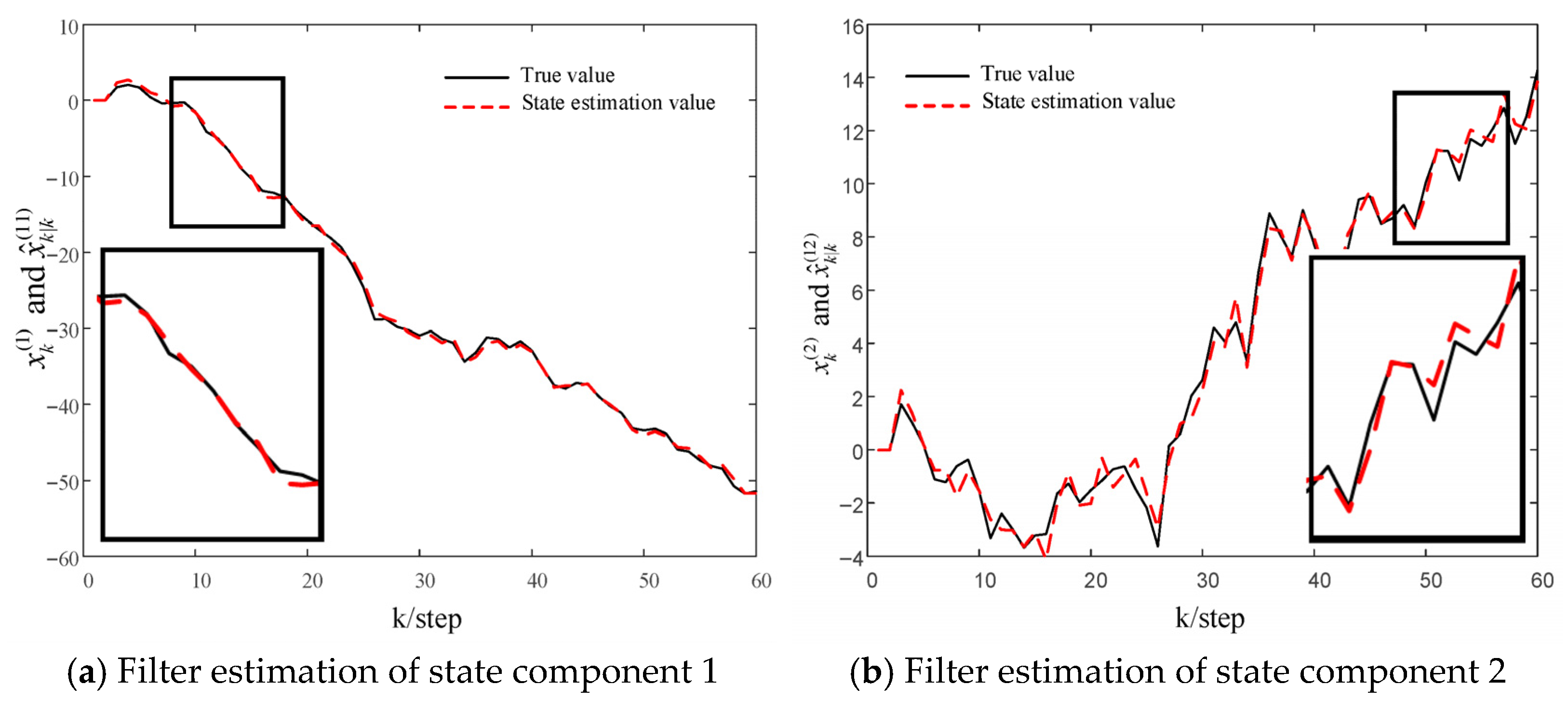
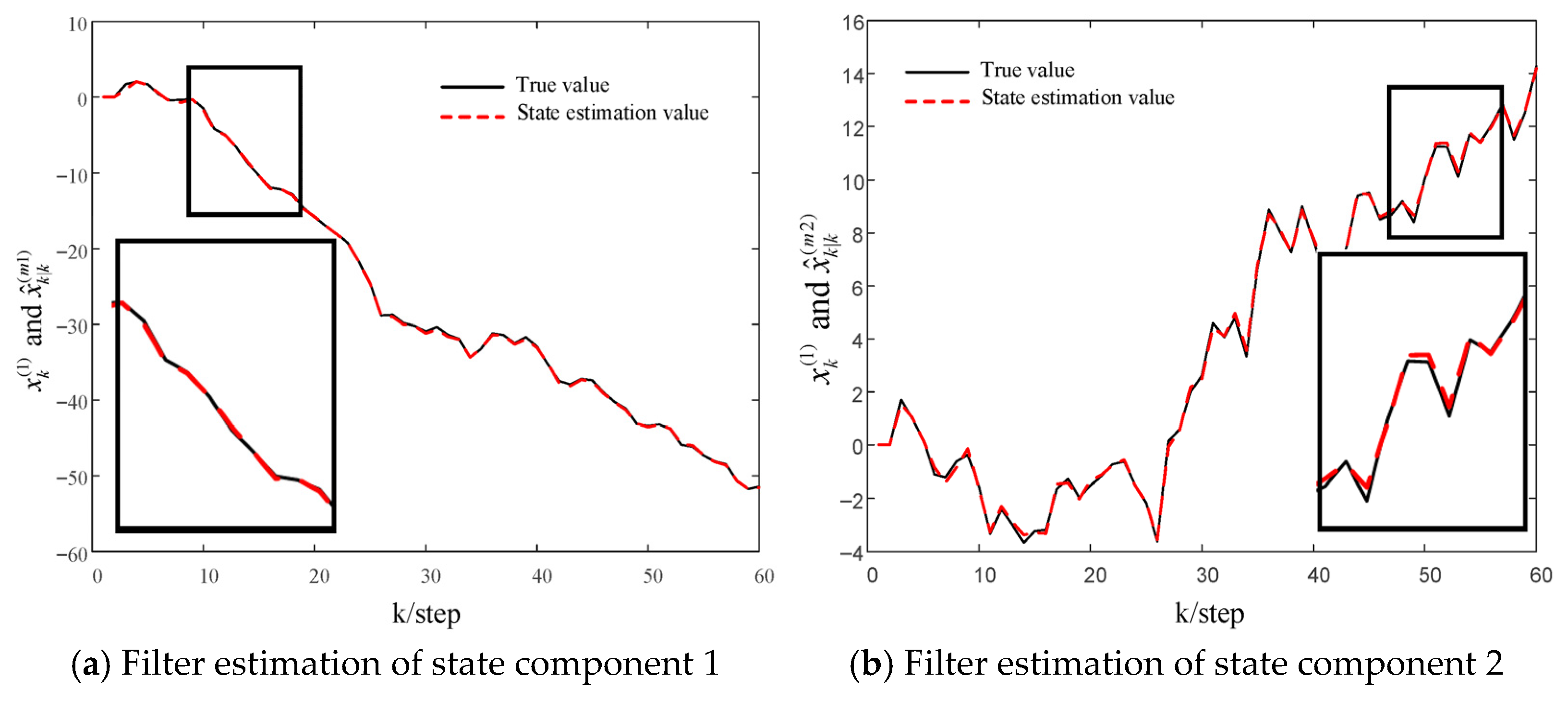
Figure 1 shows the state estimation values ${\widehat{x}}_{k|k}^{\left(1\right)}=[\begin{array}{cc}{\widehat{x}}_{k|k}^{\left(11\right)}& {\widehat{x}}_{k|k}^{\left(12\right)}\end{array}{]}^T$ obtained by applying the state augmentation method in Section 3.1 to local sensor 1. Figure 2 shows the state estimation values ${\widehat{x}}_{k|k}^{\left(1\right)}=[\begin{array}{cc}{\widehat{x}}_{k|k}^{\left(11\right)}& {\widehat{x}}_{k|k}^{\left(12\right)}\end{array}{]}^{\mathrm{T}}$ obtained by applying the non-state augmentation method in Section 3.2 to local sensor 1. The dashed lines in the figure represent different degrees of fit, resulting in varying estimation accuracies. The local curves in the figure have been enlarged, making the distinctions more apparent. From Figure 1 and Figure 2, it can be seen that the two local delay fractional order filters proposed in this paper have good estimation performance, and the local filter based on the state augmentation method has better performance.

In order to compare the accuracy of the two methods more intuitively, Figure 3 conducts 300 Monte Carlo experiments on the filters obtained by the two methods based on local sensors 1, 2, and 3. The Monte Carlo experiments show that the accuracy of local non-augmented delay fractional order filters is lower than that of local state augmented delay fractional order filters, but the error is within a very small range. At the same time, after comparing the amount of error variance calculation, the first method requires 432 multiplication and division operations per time, while the second method only requires 16 multiplication and division operations per time. It can be seen that compared to the state augmentation method, the non-state augmentation method has a lower accuracy, but it avoids the increase in system dimensionality and is more suitable for practical applications.

Figure 4 shows the state estimation values ${\widehat{x}}_{k|k}^{\left(i\right)}=[\begin{array}{cc}{\widehat{x}}_{k|k}^{\left(i1\right)}& {\widehat{x}}_{k|k}^{\left(i2\right)}\end{array}{]}^T, i=1, 2, 3$ obtained based on the non-state augmentation method, and the three-sensor distributed fusion filter estimation obtained through matrix weighted fusion. Compared with Figure 1 and Figure 2, the estimated curve in Figure 4 fits the true value line better, and they are almost overlapping. It can be seen that the accuracy of the fusion filter is further improved compared to the local filter.

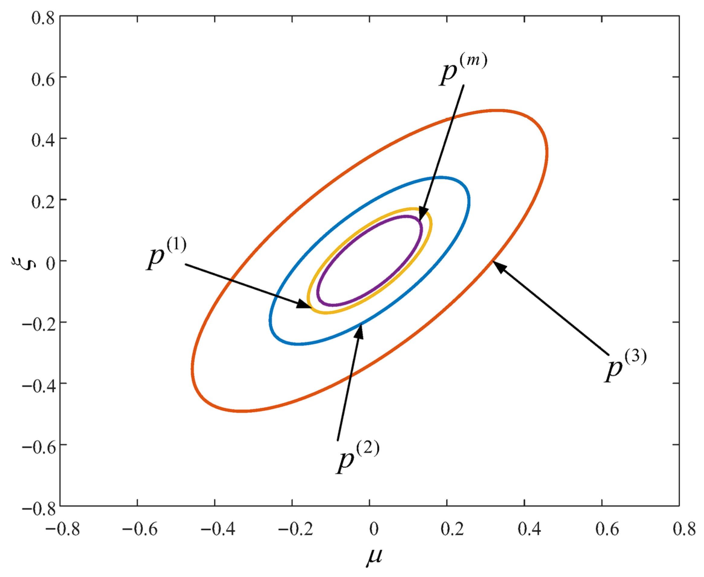
Figure 5 shows the error variance ellipse of multi-sensor local and fusion $\left\{\right[\mu \hspace{0.33em}\xi \left]\right(P^{\left(i\right)}{)}^{-1}[\mu \hspace{0.33em}\xi {]}^T\le 1\}$, $i=1, 2, 3, m$ and the error ellipse curve of the matrix fusion filter in the figure is included in the error ellipse curve of the local filter.

Table 1. Comparison of traces for weighted fusion suboptimal filtering and state augmented optimal filtering.

Trace	$\mathbf{t}\mathbf{r} \mathbf{\left(}{\mathit{P}}^{\mathbf{\left(}\mathbf{21}\mathbf{\right)}}\mathbf{\right)}$	$\mathbf{t}\mathbf{r} \mathbf{\left(}{\mathit{P}}^{\mathbf{\left(}\mathbf{22}\mathbf{\right)}}\mathbf{\right)}$	$\mathbf{t}\mathbf{r} \mathbf{\left(}{\mathit{P}}^{\mathbf{\left(}\mathbf{23}\mathbf{\right)}}\mathbf{\right)}$	$\mathbf{t}\mathbf{r} \mathbf{\left(}{\mathit{p}}^{\mathbf{\left(}\mathbf{11}\mathbf{\right)}}\mathbf{\right)}$	$\mathbf{t}\mathbf{r} \mathbf{\left(}{\mathit{p}}^{\mathbf{\left(}\mathbf{12}\mathbf{\right)}}\mathbf{\right)}$	$\mathbf{t}\mathbf{r} \mathbf{\left(}{\mathit{p}}^{\mathbf{\left(}\mathbf{13}\mathbf{\right)}}\mathbf{\right)}$	$\mathbf{t}\mathbf{r} \mathbf{\left(}{\mathit{p}}^{\mathbf{\left(}\mathit{m}\mathbf{\right)}}\mathbf{\right)}$
Value	0.0430	0.0941	0.2795	0.0542	0.1402	0.4513	0.0392

provides a comparison of the traces of local filters and fusion filters, among them, $tr\left(P^{\left(11\right)}\right)$, $tr\left(P^{\left(12\right)}\right)$, and $tr\left(P^{\left(13\right)}\right)$ are the values of the local filter 1–3 traces based on the augmented method, respectively, $tr\left(p^{\left(21\right)}\right)$, $tr\left(p^{\left(22\right)}\right)$ and $tr\left(p^{\left(23\right)}\right)$ are the values of local filters 1–3 traces based on non augmented methods, respectively, $tr{p}_m$ is the value of the weighted fusion fractional order filter trace. From Figure 5 and Table 1, it can be more intuitively seen that the matrix weighted distributed fusion filter has higher accuracy, and the accuracy relationships are $tr\left(p^{\left(21\right)}\right)<tr\left(p^{\left(11\right)}\right)$, $tr\left(p^{\left(22\right)}\right)<tr\left(p^{\left(12\right)}\right)$, $tr\left(p^{\left(23\right)}\right)<tr\left(p^{\left(13\right)}\right)$ and $tr\left(p^{\left(m\right)}\right)<tr\left(p^{\left(21\right)}\right)<tr\left(p^{\left(22\right)}\right)<tr\left(p^{\left(23\right)}\right).$

6. Conclusions

In this paper, two types of local Kalman filters were proposed for the multi-sensor fractional order time-delay systems. By employing the augmented state algorithm, the time-delay system was transformed into a non-time-delay system. To alleviate the computational burden, another Kalman filtering algorithm was put forward. This algorithm was based on substituting smoothing with filtering approximation during the calculation of the estimated values of observation predictions. Simultaneously, the calculation formulas for the local estimation error covariance matrices were provided, and the multi-sensor time-delay fractional order Kalman fuser was obtained via weighted fusion. Ultimately, the simulation results demonstrated the effectiveness and feasibility of the proposed algorithm.

The future studies are given as follows:

• Different fusion algorithms can be applied in the multi-sensor time-delay fractional system.
• More complex time-delay situation can be taken into account.
• The practical applications of the proposed algorithms in this paper can be studied.

References

1. Sauer, R.A.; Ghaffari, R.; Gupta, A. The multiplicative deformation split for shells with application to growth, chemical swelling, thermoelasticity, viscoelasticity and elastoplasticity. Int. J. Solids Struct. 2019, 2019, 53–68. [Google Scholar] [CrossRef]
2. Marouf, A.; Pudlo, P.; Sentouh, C.; Djemai, M. Investigation of the driver’s arm viscoelastic properties during steering vehicle maneuver. IEEE Trans. Syst. Man Cybern. 2017, 47, 1030–1036. [Google Scholar] [CrossRef]
3. Cao, T.N.; Trinh, D.P.; Jeong, Y.; Shin, H. Anomalous diffusion in molecular communication. IEEE Commun. Lett. 2015, 19, 1674–1677. [Google Scholar] [CrossRef]
4. Song, P.F.; Wei, P.J.; Zhou, X.L. Free Vibration of Four Sided Fixed Supported Plates on Fractional Viscoelastic Pasternak Foundation. Mech. Q. 2022, 43, 681–690. [Google Scholar]
5. Wu, Y.L.; Chen, S.; Yin, T.T. GNSS/INS Tightly Coupled Navigation with Robust Adaptive Extended Kalman Filter. Int. J. Automot. Technol. 2023, 23, 1639–1649. [Google Scholar] [CrossRef]
6. Limaverde Filho, J.O.A.; Fortaleza, E.L.F.; Silva, J.G.; de Campos, M.C.M.M. Adaptive Kalman filtering for closed-loop systems based on the observation vector covariance. Int. J. Control 2022, 95, 1731–1746. [Google Scholar] [CrossRef]
7. Zhang, G.W.; Yin, J.Y.; Deng, P.; Sun, Y.; Zhou, L.; Zhang, K. Achieving Adaptive Visual Multi-Object Tracking with Unscented Kalman Filter. Sensors 2022, 22, 9106. [Google Scholar] [CrossRef]
8. Fei, T.; Lu, C. Adaptive fractional order sliding mode controller with neural estimator. J. Frankl. Inst. 2018, 355, 2369–2391. [Google Scholar] [CrossRef]
9. Najar, S.; Abdelkrim, M.N.; Abdelhamid, M.; Aoun, M. Discrete fractional Kalman filter. IFAC Proc. Vol. 2009, 42, 520–525. [Google Scholar] [CrossRef]
10. Chen, Y.Q.; Moore, K.L. Discretization schemes for fractional-order differentiators and integrators. IEEE Trans. Circuits Syst. I Fundam. Theory Appl. 2002, 49, 363–367. [Google Scholar] [CrossRef]
11. Wu, X.; Sun, Y.; Lu, Z.; Wei, Z.; Ni, M.; Yu, W. A modified Kalman filter algorithm for fractional system under Levy noises. J. Frankl. Inst. 2015, 352, 1963–1978. [Google Scholar] [CrossRef]
12. Sun, Y.; Wu, X.; Cao, J.; Wei, Z.; Sun, G. Fractional extended Kalman filtering for non-linear fractional system with Lévy noises. IET Control Theory Appl. 2016, 11, 349–358. [Google Scholar] [CrossRef]
13. Gao, Z.; Huang, X.M.; Chen, X.J. Kalman filter design for fractional order systems with fractional order colored correlated noises. Control Decis. 2021, 36, 1672–1678. [Google Scholar]
14. Zhang, Y.G. Adaptive Filtering, Prediction and Control. Control. Theory Appl. 1986, 3, 122–123. [Google Scholar]
15. Hassibi, B.; Kailath, T.; Sayed, A.H. Linear Estimation; Prentice Hall: Upper Saddle River, NJ, USA, 2000; pp. 61–77. [Google Scholar]
16. Liang, D.F. On Continuous-time Estimation for Linear Delayed-systems with Correlated State and Observation Noises. IEEE Trans. Autom. Control 1977, 22, 472–474. [Google Scholar] [CrossRef]
17. Lu, X.; Zhang, H.; Wang, W.; Teo, K.-L. Kalman filtering for multiple time-delay systems. Automatica 2005, 41, 1455–1461. [Google Scholar] [CrossRef]
18. Torabi, H.; Pariz, N.; Karimpour, A. Kalman filters for fractional discrete-time stochastic systems along with time-delay in the observation signal. Eur. Phys. J. Spec. Top. 2016, 225, 107–118. [Google Scholar] [CrossRef]
19. Azami, A.; Naghavi, S.V.; Tehrani, R.D.; Khooban, M.H.; Shabaninia, F. State estimation strategy for fractional order systems with noises and multiple time delayed measurements. IET Sci. Meas. Technol. 2017, 11, 9–17. [Google Scholar] [CrossRef]
20. Li, J.J.; Yuan, G.J.; Fan, H. Multispectral Image Fusion Using Fractional-Order Differential and Guided Filtering. IEEE Photonics J. 2019, 11, 7801718. [Google Scholar] [CrossRef]
21. Zhao, W.D.; Lu, H.C. Medical Image Fusion and Denoising with Alternating Sequential Filter and Adaptive Fractional Order Total Variation. IEEE Trans. Instrum. Meas. 2017, 66, 2283–2294. [Google Scholar] [CrossRef]
22. Lin, K.R. Analysis and comparison of several different definitions of fractional derivative. J. Minjiang Univ. 2003, 24, 3–6. [Google Scholar]
23. Xue, D.Y.; Zhao, C.N. Simulation method and application of fractional order nonlinear system based on block diagram. J. Syst. Simul. 2006, 18, 2405–2408. [Google Scholar]
24. Anderson, B.D.O.; Moore, J.B. Optimal Filtering; Prentice Hall: Upper Saddle River, NJ, USA, 1979; pp. 36–46. [Google Scholar]
25. Deng, Z.L.; Wang, X.; Gao, Y. Modeling and Estimation; Science Press: Beijing, China, 2007; pp. 125–128. [Google Scholar]
26. Sun, S.L.; Deng, Z.L. Multi-sensor optimal information fusion Kalman filter. Automatica 2004, 40, 1017–1023. [Google Scholar] [CrossRef]
Figure 1. State x ( k ) and Local filter based on state augmentation method x ^ ( 1 ) ( k | k ) .
Electronics 14 03745 g001
Figure 2. State x ( k ) and Suboptimal local filter x ^ ( 1 ) ( k | k ) .
Electronics 14 03745 g002
Figure 3. Comparison of MSE between locally non-augmented fractional order filter and locally augmented fractional order filter.
Electronics 14 03745 g003
Figure 4. State x ( k ) and Weighted fusion suboptimal Kalman filtering x ^ ( m ) ( k | k ) .
Electronics 14 03745 g004
Figure 5. Comparison curve of suboptimal non-augmented Kalman filtering error variances.
Electronics 14 03745 g005