A Hybrid Deep Learning and Optical Flow Framework for Monocular Capsule Endoscopy Localization

Abstract

Pose estimation and localization within the gastrointestinal tract, particularly the small bowel, are crucial for invasive medical procedures. However, the task is challenging due to the complex anatomy, homogeneous textures, and limited distinguishable features. This study proposes a hybrid deep learning (DL) method combining Convolutional Neural Network (CNN)-based pose estimation and optical flow to address these challenges in a simulated small bowel environment. Initial pose estimation was used to assess the performance of simultaneous localization and mapping (SLAM) in such complex settings, using a custom endoscope prototype with a laser, micromotor, and miniaturized camera. The results showed limited feature detection and unreliable matches due to repetitive textures. To improve this issue, a hybrid CNN-based approach enhanced with Farneback optical flow was applied. Using consecutive images, three models were compared: Hybrid ResNet-50 with Farneback optical flow, ResNet-50, and NASNetLarge pretrained on ImageNet. The analysis showed that the hybrid model outperformed both ResNet-50 (0.39 cm) and NASNetLarge (1.46 cm), achieving the lowest RMSE of 0.03 cm, with feature-based SLAM failing to provide reliable results. The hybrid model also gained a competitive inference speed of 241.84 ms per frame, outperforming ResNet-50 (316.57 ms) and NASNetLarge (529.66 ms). To assess the impact of the optical flow choice, Lucas–Kanade was also implemented within the same framework and compared with the Farneback-based results. These results demonstrate that combining optical flow with ResNet-50 enhances pose estimation accuracy and stability, especially in textureless environments where traditional methods struggle. The proposed method offers a robust, real-time alternative to SLAM, with potential applications in clinical capsule endoscopy. The results are positioned as a proof-of-concept that highlights the feasibility and clinical potential of the proposed framework. Future work will extend the framework to real patient data and optimize for real-time hardware.

1. Introduction

Endoscopy is a medical procedure that enables doctors to evaluate and visualize the interiors of the body cavities in the gastrointestinal (GI) tract. New technologies like wireless capsule endoscopy (WCE) have recently surfaced, which cause the patient very little discomfort [1]. However, existing capsule endoscopes do not allow for control over movement or orientation; instead, they move passively, depending only on intestinal peristalsis [2,3]. Accurate and reliable determination of the location of capsule endoscopy (CE) in the gastrointestinal system both increases the accuracy of diagnosis and directly affects the effectiveness of the treatment process. Localization also contributes to the monitoring of the capsule’s progression, transit time analysis, and evaluation of intestinal motility disorders. In this context, studies on CE localization play a critical role in modern medicine in terms of both diagnosis and treatment.

Currently, the position of the capsule is determined by different wearable sensors and radio frequency (RF) triangulation in the 3D abdomen. In addition, various alternative methods, which are also sensor-based, have been proposed [4,5]. However, these methods can only determine the location of CE within the abdominal cavity in 2D or 3D and cannot provide information about its location within the GI tract. On the other hand, visual-based approaches are in the early stages for intraluminal localization and have shown promising results [6,7]. Recent advances in artificial intelligence (AI) increasingly contribute to CE analysis and prove its high accuracy and reliability in medical image analysis [8]. While traditional geometry-based methods require manually designed features to provide matching between images, such as Visual SLAM (V-SLAM), DL-based localization, mapping, and reconstruction methods can perform end-to-end feature learning over large datasets [3,9]. In this context, techniques such as DL-based SLAM [10,11], Structure from Motion (SfM) [12,13], and Neural Field Rendering [14,15] offer significant potential in endoscopic applications in body cavities [3].

In this study, a hybrid DL and optical flow framework is proposed for six-degree-of-freedom (6-DoF) pose estimation and localization task for CE applications in an environment with homogeneous texture, repetitive visual patterns, and limited distinctive features, such as the small intestine. First, pose estimation was performed using Oriented FAST and Rotated BRIEF (ORB) and Scale-Invariant Feature Transform (SIFT)-based feature extraction and classical V-SLAM algorithms; however, it was observed that these methods did not perform sufficiently in this complex environment, and the feature matches were insufficient and unstable. Therefore, in order to overcome the cases where V-SLAM failed, a CNN-based hybrid approach enriched with optical flow (Farneback) was developed and evaluated in a test environment. Within the scope of the study, it was demonstrated that the proposed hybrid model showed superior performance with lower RMSE and faster inference time compared to traditional DL architectures such as ResNet-50 and NASNetLarge. In this context, the developed framework offers a promising alternative for clinical CE applications where real-time and accurate localization is critical.

This study consists of six sections. In the introduction, the importance of CE localization and the inadequacies of the existing methods are explained. In the related studies, SLAM and AI-based approaches are examined, and gaps in the literature are highlighted. In the methodology, classical V-SLAM, Farneback optical flow, and DL architectures (ResNet-50, NASNetLarge) are introduced, and the proposed hybrid method is detailed. In the implementation section, the developed techniques are applied in a test environment, and the results are compared with other methods. In the results and discussion, the models are compared in terms of RMSE, training time, and inference time, and the superior performance of the hybrid model is demonstrated. Finally, in the conclusion, the general contribution of the study is summarized, and suggestions for future developments are included.

2. Related Studies

The related study can be summarized in two categories in terms of CE localization: classical V-SLAM methods and AI applications. Although there are many literature reviews addressing the revolutionary role of AI in modern endoscopy practices, most of these studies focus only on image recognition and segmentation techniques, such as computer-aided diagnosis (CADx) and lesion detection. DL-based localization, mapping, and 3D reconstruction are rarely addressed in [3]. A performance evaluation of SLAM algorithms commonly used in endoscopy is presented in [16], but the discussion is limited to geometric-based SLAM methods only. Similarly, [17] also addresses the issue of endoscopic 3D reconstruction only within the framework of traditional methods such as shape from shading (SfS) and SfM.

On the other hand, [10] proposes a CNN-based system that performs 6-DoF pose estimation for CE using only monocular camera images. Tested on a realistic human stomach model, the system achieved high accuracy with 7.1% position and 3.4% orientation error. It achieved robust results even in endoscopic environments with low resolution, distorted, and repetitive textures. Different feature descriptors, such as SIFT, SURF, Local Intensity Order Pattern (LIOP), Maximally Stable External Regions (MSER), and DL-based PWC-Net, were compared, and the best results in visual matching were obtained with PWC-Net in [18]. It has been stated that AI-based approaches offer significant advantages in real-time motion tracking, and CNN-based feature descriptors give successful results even in poorly textured, inhomogeneous illumination environments in [19]. In addition, the triangle matching algorithm proposed by [20] performed the soft tissue surface tracking task with a depth matching network trained on speckle matching data. It showed promise in terms of precise navigation for endoscopic robots. The real-time and reliable 3D pose estimation problem required for the control of active CE robots is addressed, and a transformer-based architecture for position and depth estimation is proposed in [21]. The model aims to cope with these complex structures by using the self-attention mechanism against challenges such as the deformable structure of the gastrointestinal system and specular reflections occurring on non-textured surfaces. This approach, developed by taking advantage of the success of the transformer architecture in visual tasks, contributes to the development of fully autonomous CE systems for advanced diagnostic and therapeutic procedures by providing a more precise determination of the capsule position.

3. Methodology

3.1. V-SLAM

The main aim in V-SLAM systems is to accurately determine the location of the robot, which is one of the most critical stages of the entire process [22]. This process includes a number of important steps required for the robot to detect its location successfully. A particularly prominent step is feature tracking, which involves tasks such as feature extraction, matching, re-localization, and pose estimation [23]. These steps help align and define frames to ensure the creation of the first key frame of the input data [24]. The key frame consists of image frames that contain the observed feature points and the camera poses together. This structure plays an important role in tracking and positioning processes and contributes to the elimination of drift errors in the camera poses on the robot [25,26]. This key framework is then transferred to the next stage to create the preliminary map [27,28,29].

3.2. Farneback Optical Flow

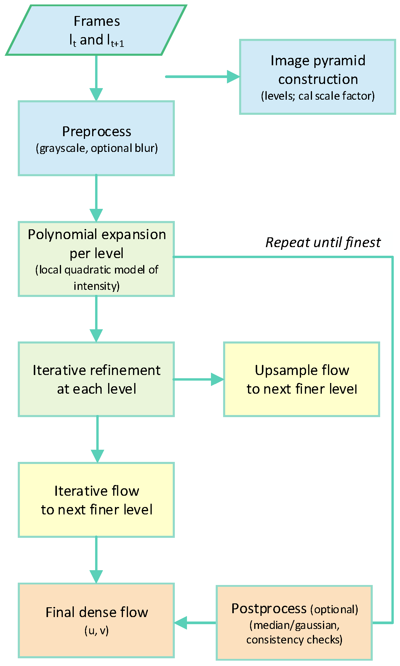
In this study, the Farneback dense optical flow algorithm (OpenCV implementation) was used for inter-frame motion estimation. This algorithm calculates dense displacement fields by modeling pixel neighborhoods with a polynomial expansion and using a pyramidal approximation. The parameters were not specifically modified, and the default OpenCV values, which are widely used in the literature, were used. This achieved reliable performance in low-texture environments. A block diagram summarizing the basic processing steps of the algorithm is presented in Figure 1.

The Farneback method treats an image as a two-dimensional signal. In this approach, the value of each pixel in the image is considered as a function of a two-dimensional variable. A local coordinate system is defined in which each pixel is considered as the center, and this function is approximated by a quadratic polynomial in Equation (1), [30]:

$$f\left(x\right)=x^{T}Ax+b^{T}x+c$$

(1)

A is a symmetric matrix of dimensions 2 × 2, b is a vector of dimensions 2 × 1, and c is a constant coefficient. These coefficients are estimated using the least squares method, taking into account the neighboring pixels around each pixel.

The new function obtained as Equation (2), after the pixel is displaced by d is

$$f_2\left(x\right)={\left(x-d\right)}^T{A}_1\left(x-d\right)+b_1^T\left(x-d\right)+C_1$$

(2)

Farneback uses the following relationships to find the motion vector d:

$$A_2=A_1$$

(3)

$$b_2=b_1-2A_{1}d$$

(4)

$$C_2=d^T{A}_{1}d-b_1^{T}d+C_1$$

(5)

Based on Equations (3)–(5), the displacement vector is obtained as Equation (6), [30]:

$$d=-{\displaystyle \frac{\left(b_2-b_1\right)}{2}}$$

(6)

A₁ is the symmetric estimation of the local second-order coefficients; (b₂ − b₁) represents the difference in the linear terms obtained from two consecutive frames.

3.3. Lucas–Kanade Optical Flow

Optical flow, first introduced by Gibson in 1950, is a vector field that expresses the instantaneous motion of an object in a scene on the image plane. The basic idea is to use pixel changes and inter-frame correlation between consecutive frames to find correspondences between the last frame and the current frame, thereby extracting motion information. Optical flow can be generated by target motion, camera motion, or a combination of both; computational approaches generally fall into three categories: region/feature-based matching, frequency-domain, and gradient-based methods. In principle, a velocity vector is assigned to each pixel, resulting in a motion vector field; points in the image correspond to 3D object points via projection. While the vectors are continuous in the scene when there is no moving object, the vectors diverge when there is relative motion between the target and the background. The target’s position is calculated from this difference. Once the position is found, the target is tracked iteratively by observing the vertex/feature relationships in consecutive frames [31].

3.4. DL Architectures

3.4.1. ResNet-50 Model

ResNet is one of the most widely used CNN architectures. CNN architectures generally consist of convolution layers, pooling layers, and fully connected layers. In addition, operations such as zero padding, Rectified Linear Unit (ReLU) activation function, and batch normalization are integrated into these structures in order to increase the accuracy rate. The most important advantage of ResNet is that it can solve the vanishing gradient problem. This success is achieved thanks to the residual block structure that adds a “shortcut” to each layer. These blocks allow gradients to reach the first layers of the network more effectively. In this way, performance degradation is prevented as the depth increases [32].

There are different versions of ResNet: ResNet-50, ResNet-101, and ResNet-152. The basic structure in these architectures starts with the processing of the input image with a convolutional layer. The convolution operation is the systematic application of a filter matrix (kernel) to the image and is defined by Equation (7), [32]:

$$G\left[m,n\right]=\left(f\ast h\right)\left[m,n\right]=\sum _j^{x}x\sum _k^{x}h\left[j,k\right]·f\left[m-j,n-k\right]$$

(7)

Following deep learning practice, we implement ‘convolution’ as cross-correlation without kernel flipping; for mathematical completeness, the classical convolution is also defined above.

In Equation (8), f is the input image, h is the filter, and m and n are the row and column indices.

$$f\left(x\right)=\mathrm{m}\mathrm{a}\mathrm{x}\left(0,x\right)$$

(8)

After each convolution layer, the ReLU activation function is usually applied. This function sets negative values equal to zero and preserves positives, allowing the model to learn faster and more effectively. The subsequent pooling layer, especially max pooling, reduces the spatial dimension and lightens the computational burden by taking the maximum value at each filter position, thus obtaining a more concise representation of the image features. Finally, the average pooling layer reduces the image by taking the average value in each region. The fully connected layer that follows makes the resulting feature map ready for classification [32].

3.4.2. Neural Architecture Search Network (NASNet) Model

Google Brain developed the NASNet model in 2018 [33]. The NASNetLarge model, which is a pretrained model from the NASNet architecture family, eliminates the need to design a model according to the dataset manually, thanks to its ability to automatically generate the network structure. This architecture offers the advantage of reducing the number of parameters without compromising accuracy. The basic search method used in the pretrained model of NASNet is the NAS Framework [34], and this structure consists of CNN [35] and Control Recurrent Neural Network (CRNN) components. CRNN evaluates the performance of CNN-based subnetworks (Child Network) and optimizes the structure of the model through reinforcement learning (RL) [36,37].

3.5. Hybrid CNN–Optical Flow Approach

This section presents the proposed hybrid framework for monocular 3D pose estimation for CE. The approach combines the strengths of a CNN for pose regression and a geometric optical flow algorithm for short-term motion refinement.

3.5.1. CNN-Based Absolute Pose Regression

The core of our method is a DL model based on the ResNet-50 architecture pretrained on the ImageNet dataset. The final classification layer of ResNet-50 is replaced with a custom regression head comprising fully connected layers, as in Equation (9), that outputs a 6-DoF pose vector:

$$p=\left[x,y,z,\phi ,\theta ,\psi \right]$$

(9)

(x, y, z) represents the 3D translation of the camera, and (φ, θ, $\psi$) is its rotation in roll, pitch, and yaw, respectively.

The following phases make up the suggested pipeline:

The input images are converted from BGR to RGB.

The images are downsized to 224 by 224 pixels.

The normalization procedure makes use of the ImageNet mean and standard deviation values.

Pose regression predicts an absolute 6-DoF pose.

Images were converted from BGR to RGB to ensure compatibility with the deep learning framework (PyTorch/TensorFlow), which requires RGB input.

Each frame is processed independently, which may lead to temporal drift and inconsistency in sequential predictions, particularly in visually repetitive or homogeneous environments like the small bowel.

3.5.2. Optical-Flow-Based Relative Motion Estimation

This study uses the Farneback dense optical flow algorithm to estimate pixel-wise motion between consecutive grayscale image frames. Farneback proposed a classical method for solving the dense optical flow problem, which allows the motion vector and contour information of the object to be obtained. Farneback optical flow is a gradient-based algorithm that uses a polynomial expansion model to estimate the motion between two frames, enabling dense optical flow computation [38]. Applications of the Farneback method have also yielded practical results; for example, [39] successfully applied this algorithm in laser speckle imaging for autonomous vessel detection [30]. In addition to our empirical observations, the literature also supports the choice of the Farneback algorithm for motion estimation tasks. For example, [40] conducted a comparative analysis of different optical flow algorithms for anomaly detection. Their results demonstrated that the Farneback algorithm outperformed Horn–Schunck and Lucas–Kanade methods in terms of execution time, while still providing reliable motion estimation. These findings further confirm the suitability of the Farneback method in applications requiring both robustness and computational efficiency.

The Farneback method computes a dense motion field by approximating neighborhoods of the image with quadratic polynomials, allowing the estimation of displacement vectors for every pixel. The steps include the following:

Grayscale conversion

Dense flow computation

Let Δx and Δy denote the mean flow in the horizontal and vertical directions, respectively. These are used to derive a corrective translation vector Δtxy, which refines the CNN-predicted translation in Equation (10):

$$t^{\prime }=t_{CNN}+\lambda \Delta t_{xy}$$

(10)

where λ ∈ [0, 1] is a fusion weight.

Equation (10) represents the general formulation of the corrective translation vector, while Equations (15) and (16) provide its component-wise weighted implementation.

3.5.3. Pose Fusion and Final Output

For each frame, the final estimated pose is computed by combining the CNN-predicted absolute pose with the optical-flow-derived relative motion:

CNN provides structure of the trajectory, including depth (z) and orientation.

Optical flow improves short-term positional accuracy, especially in lateral movement (x, y).

The final output is a smoothed pose sequence that integrates the strengths of data-driven and geometry-based estimation.

Let each input image be denoted as It at time. The goal is to estimate the 6-DoF pose Tt ∈ R⁶ in Equation (11), defined as:

$$T_t=\left[x_t,y_t,z_t,{\phi }_t,{\theta }_t,{\psi }_t\right]$$

(11)

where (x_t, y_t, z_t) are the translation components, and (φ_t, θ_t, ${\psi }_t$) represent roll, pitch, and yaw angles, respectively.

In CNN-based pose estimation, given a preprocessed image It ∈ R224 × 224 × 3, the CNN regressor f_CNN predicts the 6-DoF pose in Equations (12) and (13):

$${\widehat{T}}_t^{CNN}=f_{CNN}\left(I_t\right)$$

(12)

$${\widehat{T}}_t^{CNN}=[{\widehat{x}}_t^{CNN},{\widehat{y}}_t^{CNN},{\widehat{z}}_t^{CNN},{\widehat{\phi }}_t^{CNN},{\widehat{\theta }}_t^{CNN},{\widehat{\psi }}_t^{CNN}]$$

(13)

T denotes the general 6-DoF pose and ${\widehat{T}}_t^{CNN}$ is the estimated value predicted by CNN.

In optical-flow-based displacement, dense motion fields between consecutive grayscale images I_t−1 and I_t, were computed using Farneback optical flow. The mean displacement in x and y is calculated as in Equation (14):

$${\Delta }_{xt}^{0F}={\displaystyle \frac{1}{N}}{\sum }_{i=1}^{N}ui, {\Delta }_{yt}^{0F}={\displaystyle \frac{1}{N}}{\sum }_{i=1}^{N}vi$$

(14)

where ui and vi are the horizontal and vertical flow vectors at pixel i, and N is the total number of pixels.

A weighted average is applied for the x and y translation components, while the z and rotation components are taken from the CNN to combine the CNN and optical flow results. (Equations (15)–(18)):

$${\widehat{x}}_t=a{\widehat{x}}_t^{CNN}+\left(1-a\right)\Delta x_t^{0F}$$

(15)

$${\widehat{y}}_t=a{\widehat{y}}_t^{CNN}+\left(1-a\right)\Delta y_t^{0F}$$

(16)

$${\widehat{z}}_t={\widehat{z}}_t^{CNN}$$

(17)

$${\widehat{\phi }}_t={\widehat{\phi }}_t^{CNN},{\widehat{\theta }}_t={\widehat{\theta }}_t^{CNN},{\widehat{\psi }}_t={\widehat{\psi }}_t^{CNN}$$

(18)

In our hybrid framework, the weighted fusion is applied only to the lateral translation components (x and y). The depth (z) and all rotational components are directly taken from the CNN predictions, since our dataset labels were defined solely along the longitudinal axis with 0.5 cm increments. The fused lateral components are subsequently mapped to metric units using the scale factor defined in Equations (22) and (23). This design ensures unit consistency while reflecting the constrained geometry of the phantom setup. The full estimated pose vector is then as in Equation (19):

$${\widehat{T}}_t= [{\widehat{x}}_t,{\widehat{y}}_t,{\widehat{z}}_t, {\widehat{\phi }}_t,{\widehat{\theta }}_t,{\widehat{\psi }}_t]$$

(19)

The estimated translations are cumulatively added together to obtain the camera trajectory over time as in Equation (20):

$$P_t=P_{t-1}+\left[{\widehat{x}}_t,{\widehat{y}}_t,{\widehat{z}}_t\right]$$

(20)

with P₀ = 0 as the initial position.

Equation (20) accumulates unit-consistent translations: it is metric from the CNN supervision, while the fused lateral displacements (x,y) are scaled into centimeters according to Equations (22) and (23).

Then, the estimated translations from each frame are cumulatively added to obtain the overall trajectory of the camera using Equation (21).

$$P_t={\lambda P}_{t-1}+(1-\lambda )P_t$$

(21)

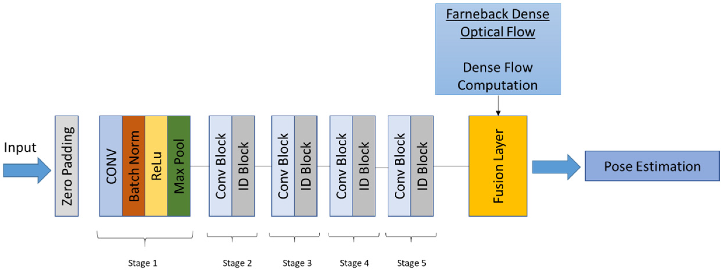
The workflow of the proposed hybrid ResNet-50–optical flow framework is shown in Figure 2.

4. Implementation

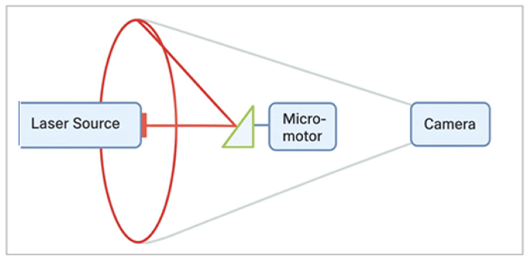
4.1. Circumferential-Scanning Endoscope

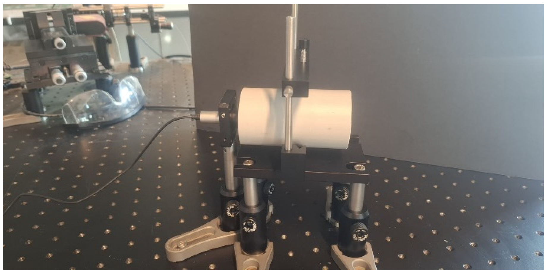
We developed a probe comprising a laser diode source, a prism located on a micromotor, and an endoscopic camera. The probe housing was established through wrapping all parts within a cylindrical and transparent protective sheath. The probe was tested on a cylindrical phantom that had arbitrarily distributed bumps at a height of 2–3 mm. The probe captured a video during a circumferential scanning operation as it was pulled through the phantom using a translational stage. For this purpose, a test area was created in the optoelectronics laboratory, in order to obtain controlled distances between image-taking points. The test area dimensions are 9 cm in height and 5 cm in width (Figure 3). The phantom was designed to mimic the morphology and texture of the jejunum segment of the small intestine, which is characterized by relatively homogeneous surface patterns.

In the test environment, the capsule is placed inside a test tube and is traversed along the longitudinal axis using a linear stage. This setup mimics the geometry of the jejunum segment of the small intestine. Figure 4 depicts the proposed capsule scheme.

4.2. SLAM Application

To benchmark our study, we evaluated the SLAM performance with monocular images obtained in our test area. In this context, monocular SLAM using ORB and SIFT features and descriptors was used separately for the localization process, utilizing a sequence of images to estimate the 3D trajectory of the camera over time, to observe the performance of SLAM in challenging environments like the small bowel. Therefore, a total of 19 images were captured during the process with 0.5 cm intervals. The photos used in the localization process are shown in Figure 5.

The first method uses ORB, a fast and efficient feature extractor and matcher, which is suitable for real-time or resource-limited applications. For each consecutive image pair, ORB features and descriptors are extracted, and these features are matched using a brute-force matcher with Hamming distance. Therefore, the relative camera motion (rotation R and translation t) using the essential matrix is obtained, and these poses are accumulated to track the camera’s estimated position in 3D space. Then, the resulting (x, y, z) positions to visualize the trajectory of the camera were stored and plotted.

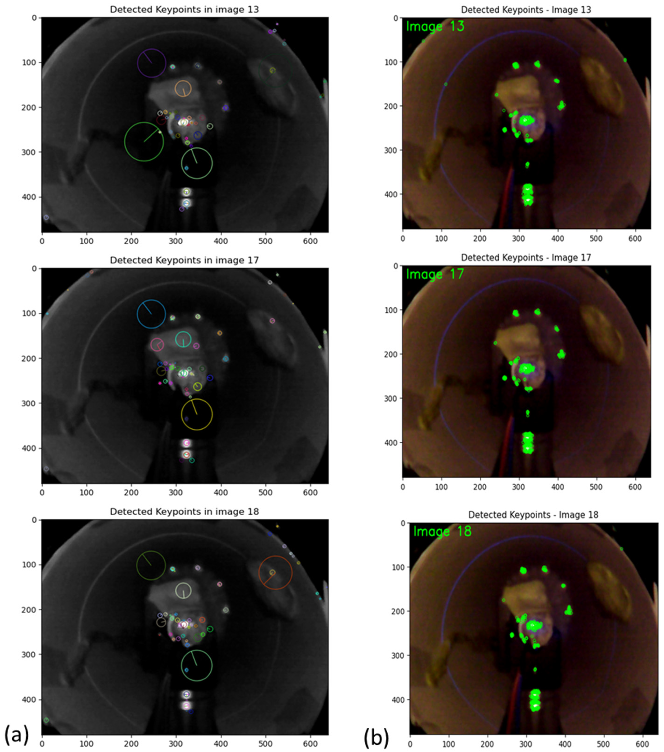
The other approach implements a basic monocular visual odometry pipeline using SIFT features and essential matrix-based pose estimation to track the 3D trajectory of a camera from sequential images. It uses SIFT to extract keypoints and descriptors from consecutive image frames. Features are matched between image pairs using a brute-force matcher, and relative camera motion (rotation and translation) is estimated via the essential matrix. The detected keypoints and matched features between consecutive images using SIFT and ORB are shown in Figure 6 and Figure 7, respectively.

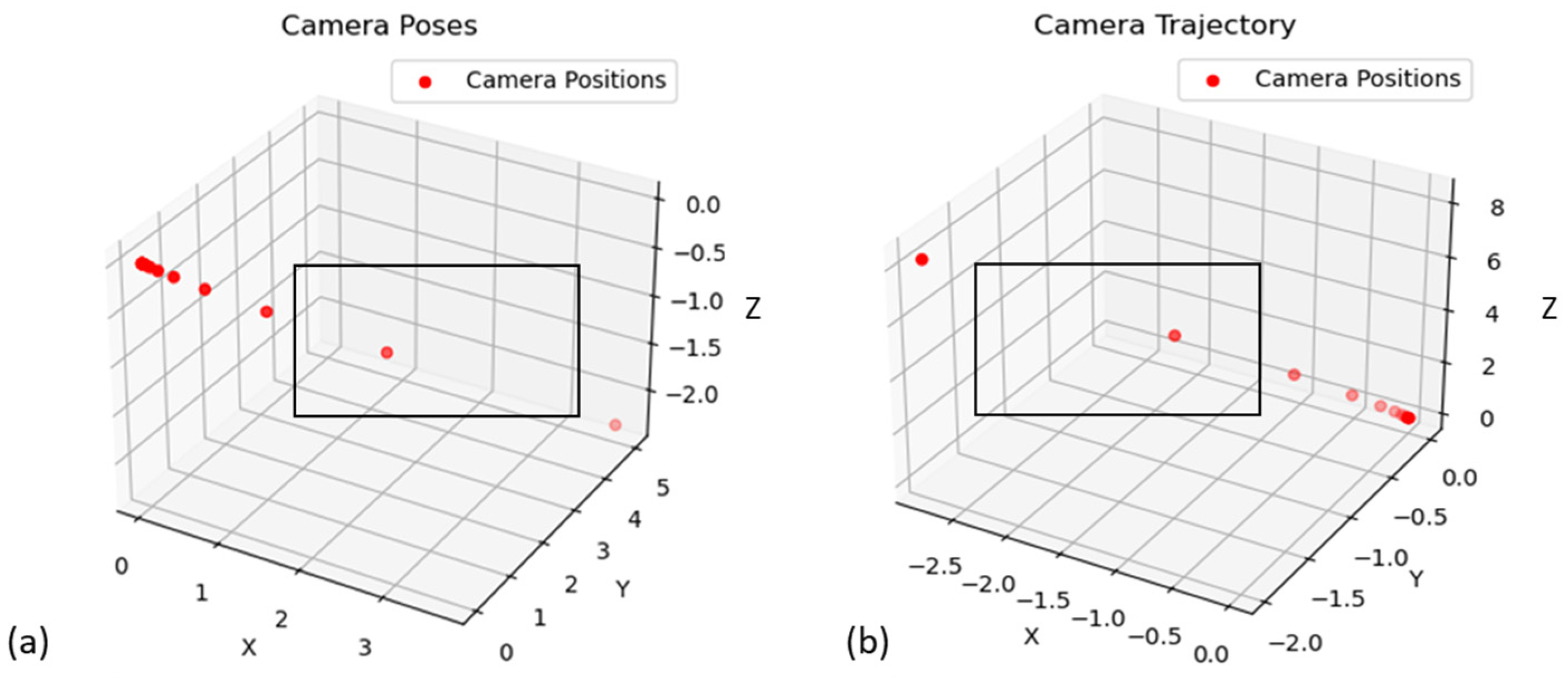
Therefore, the camera’s pose is updated incrementally over time, and the resulting 3D positions are plotted to visualize the camera path. The SLAM Localization with SIFT and ORB, respectively, is shown in Figure 8.

In the region marked with a rectangle in Figure 8, it is observed that the SLAM algorithm cannot produce the estimated camera poses. Since this region has low contrast and limited distinguishing features in the visual sense, it became difficult for the algorithm to make the necessary matches, and tracking failed. In particular, the failure to detect a sufficient number of reliable visual features between consecutive frames prevented the correct modeling of the motion and caused the localization system to fail in this area. As a result, the camera position could not be determined in this region, and a gap occurred in the estimated trajectory. This experiment confirmed that SLAM algorithms may perform poorly in such environments where visual diversity is low, repetitive patterns or homogeneous textures are dense.

4.3. Hybrid CNN and Optical Flow Application

In this application, a hybrid pose estimation framework that integrates a fine-tuned ResNet-50 CNN with classical optical flow techniques was proposed to improve localization accuracy from monocular endoscopic images and to overcome feature-based SLAM failures. Training of all CNN models was performed in the following hardware and software environment:

CPU: Intel Core i7-8750H

GPU: NVIDIA GeForce GTX 1060

RAM: 16 GB DDR4

Storage: 1 TB SSD

Python Version: 3.12.1

CUDA Version: 11.3

ResNet-50 was chosen due to its proven generalization capabilities in the medical imaging field and its robustness against over-learning. This is especially important in areas where labeled data is limited and visual similarity between classes is high, such as gastrointestinal tract images. The model architecture is based on the pretrained ResNet-50 backbone on ImageNet, where the last 30 layers are not frozen for fine-tuning. A regression head consisting of global average pooling and two dense layers predicts 6-DoF camera poses (x, y, z, roll, pitch, yaw) from preprocessed 224 × 224 RGB images.

A partial fine-tuning strategy was adopted in network training. In this strategy, the last 30 layers of the network, the upper-level residual blocks, and the regression head were left trainable, while the first layers (early-stage convolution layers) were frozen. In this way, the low-level features learned with the ImageNet dataset (edges, corners, textures) were preserved, while the higher-level layers were adapted to learn patterns specific to endoscopic images. The following precautions were taken to train the model stably and prevent over-learning:

Early stopping according to the validation dataset;

Data augmentation techniques, including random brightness variation and rotation, were applied to simulate variability.

Data augmentation on the training data is used to increase the overall accuracy of the model. Various manipulations are made on the images, including rotation, zoom, shift, brightness adjustment, and horizontal flip. These operations allow the model to be trained on a wider range of data and increase its generalization ability. The dataset is labeled as synthetic, assuming continuous forward motion of the camera along the z-axis (0.5 cm per frame) and all other pose components are initialized to zero. Therefore, the model is trained using the Adam optimizer with early stopping based on validation loss. During inference, the poses estimated by the CNN are combined with displacements derived from the Farneback dense optical flow that were computed between consecutive image pairs. To improve short-term motion estimation and reduce frame-to-frame drift, dense optical flow based on the Farneback method was calculated between consecutive grayscale image frames. Unlike sparse feature tracking, this approach estimates pixel-wise displacement across the entire image. The average values of horizontal and vertical flow vectors (Δx, Δy) were calculated to estimate planar motion. The weighted fusion method combines the predicted positions by balancing the contributions of CNN and optical flow with the parameter α. α value was determined as 0.9. In other words, 90% weight was given to CNN predictions, while 10% weight was given to optical flow. The α (alpha) value was used to optimize the accuracy of pose estimates obtained by combining the outputs of the hybrid model with CNN and optical flow data. α serves as a parameter that balances the weights of CNN and optical flow contributions. This parameter aims to improve the overall accuracy of the model by determining the weight given to the estimates of each component (CNN and optical flow).

During the study, the effect of the α value was investigated with different experiments. Initially, an equally weighted value of α = 0.5 was preferred, but as a result of the experiments, it was observed that the best performance was provided by the value of α = 0.9. Comparative experiments with different α values (0.1, 0.3, 0.5, 0.7, and 0.9) were conducted. The results revealed that α = 0.9 consistently achieved the lowest RMSE (0.03 cm), while smaller α values increased error due to reduced reliance on CNN predictions. Thus, α = 0.9 was selected as the optimal balance between CNN-based long-term stability and optical-flow-based short-term refinement. The main reason for choosing this value is that the optical-flow-based approach provides more accurate estimates in short-term movements, while the CNN model produces more reliable results in long-term estimates. The value of α = 0.9 reflects the sensitivity of optical flow to short-term movements, while balancing the stronger long-term prediction power of CNN, minimizing the total error rate.

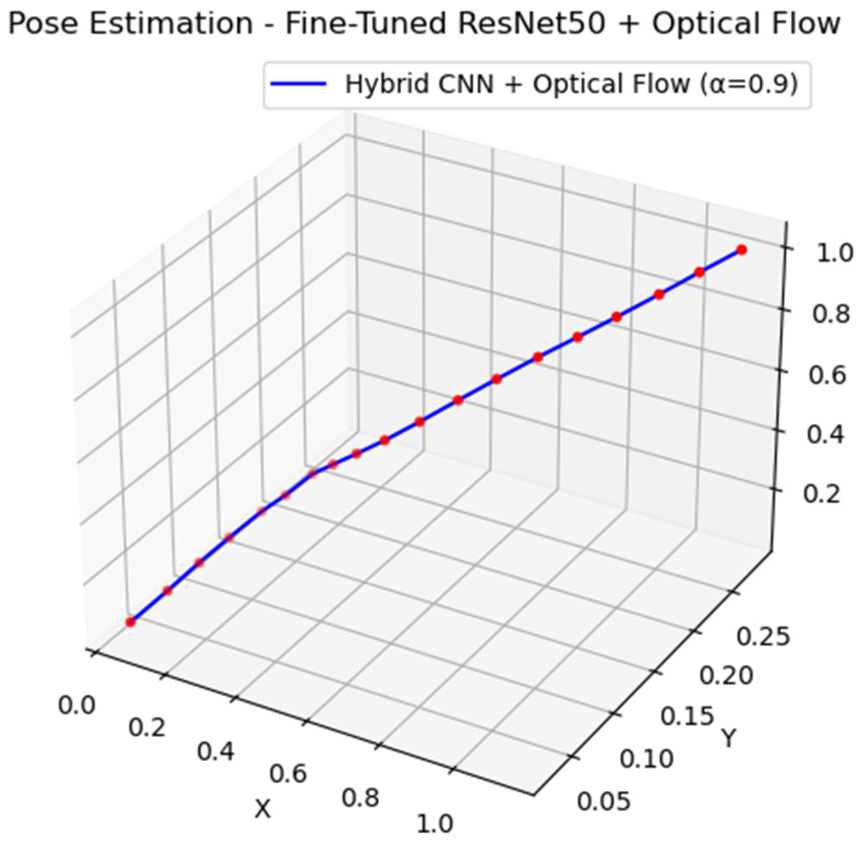
The accumulated 3D trajectory is visualized and printed to evaluate the effectiveness of the hybrid strategy in capturing the spatial progression of the camera and improves monocular pose recovery, demonstrating the benefit of combining DL with classical motion estimation.

This hybrid framework combines the structural consistency of CNN-based regression with the short-term accuracy of dense geometric motion estimation. It is particularly suitable for environments where tissue is limited and motion is complex, e.g., minimally invasive diagnostics, robotic navigation, or endoscopy. The results show that combining ResNet-50-based deep regression with dense optical flow provides improved robustness and accuracy in monocular visual localization tasks. Figure 9 demonstrates the visualization of the estimated trajectory using the CNN and optical flow hybrid pipeline.

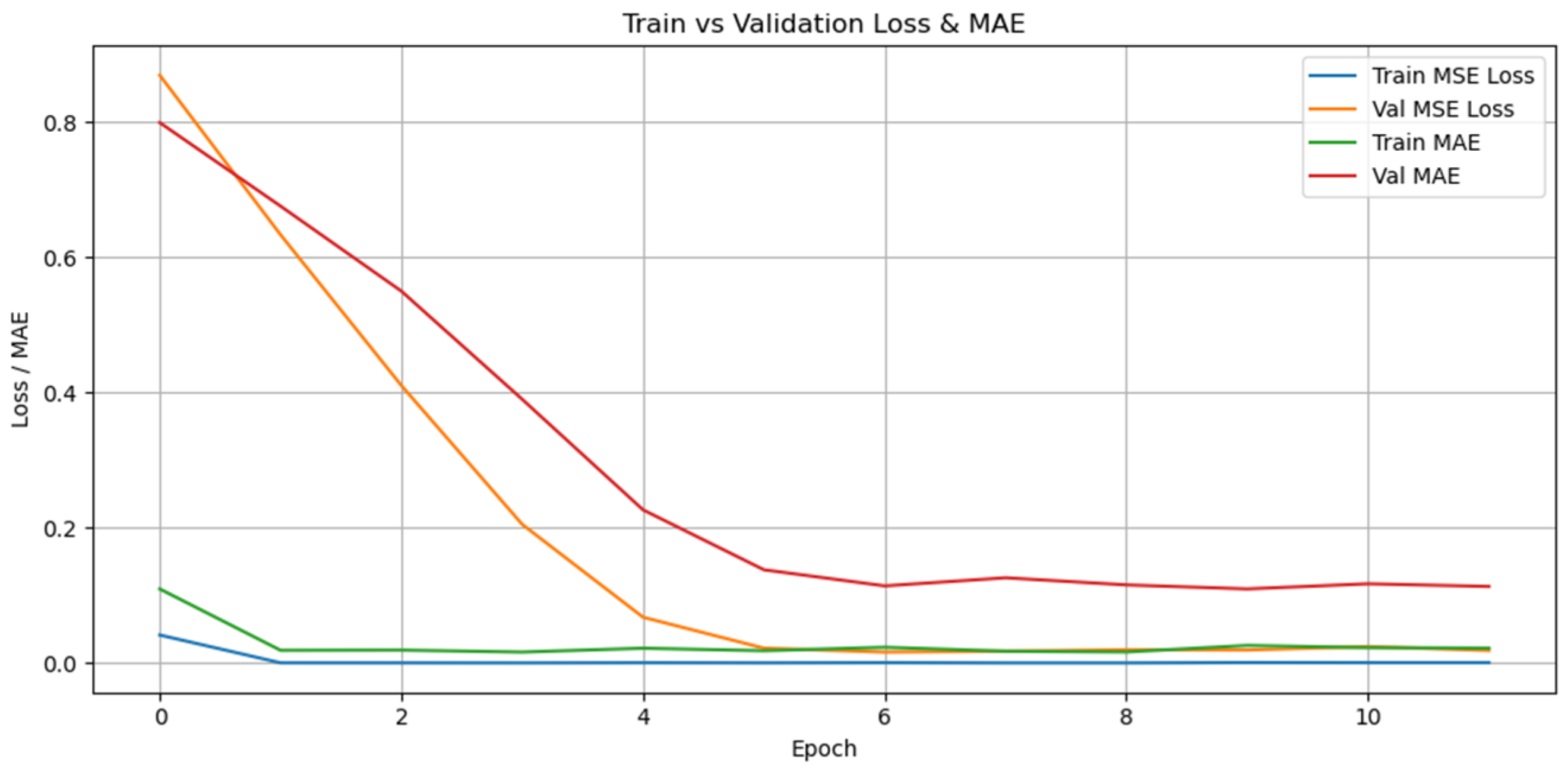
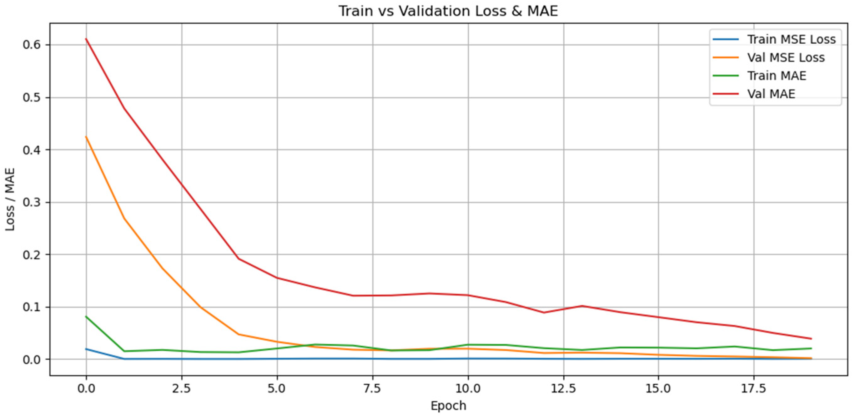
Figure 10 demonstrates the train and validation loss and Mean Absolute Error (MAE). This graph visualizes the performance of the model by comparing the MSE Loss (Mean Square Error) and MAE values on the training and validation data during the training process. In the first epochs, the training loss (Train loss) and validation loss (Val loss) are high, while both losses decrease rapidly as the training progresses.

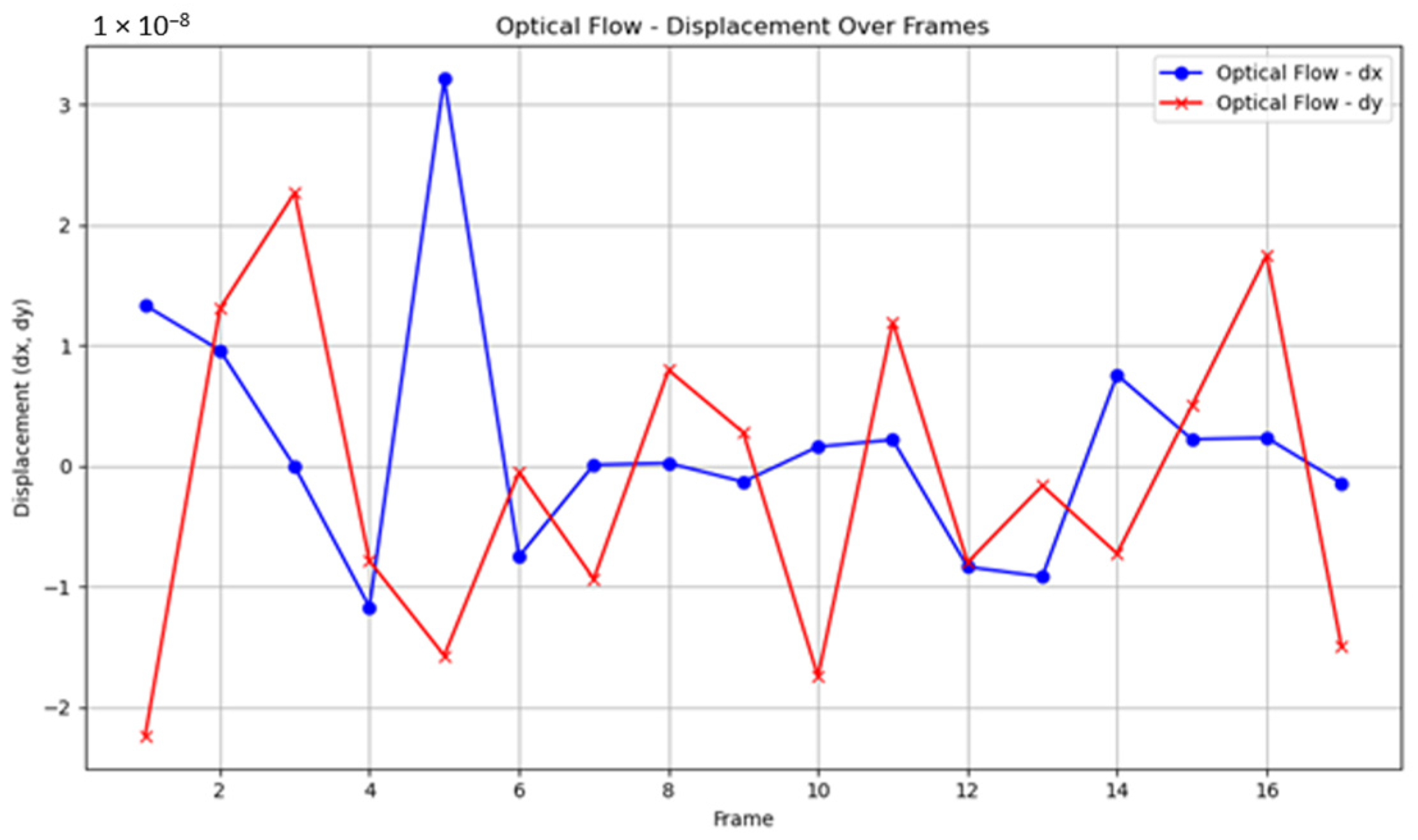
This shows that the model starts to learn on the training data and starts to make correct predictions on the validation data. Similarly, a significant decrease is observed in the Train MAE and Val MAE values, which indicates that the error in the model’s predictions decreases, i.e., the accuracy rate increases. In the later periods of the training process, the validation loss and validation MAE start to stabilize, which shows that the model does not overfit and its generalization ability is successful. As a result, the model reaches the best validation performance thanks to early stopping, while minimizing the risk of overfitting during the training process. The displacement over frames with optical flow is shown in Figure 11.

To demonstrate the performance of Farneback optical flow used in the proposed method, the same strategy is performed with Lucas–Kanade optical flow. The localization result of Resnet50 and Lucas–Kanade optical flow can be seen in Figure 12.

Figure 13 demonstrates the train and validation loss and Mean Absolute Error (MAE).

4.4. ResNet-50 and NASNetLarge Application

To evaluate the effectiveness of our proposed ResNet-50–optical-flow-based hybrid localization framework in the small bowel, the results were compared with two different baseline DL architectures; ResNet-50 and NASNetLarge with end-to-end training.

Initially, 6-DoF pose estimation was performed using a model built on a ResNet-50 architecture previously trained on ImageNet and fine-tuned with the last 30 layers of the regression head. Endoscopic images were resized, normalized, and sequentially converted to the training dataset to fit the model. Training is performed on the last 30 layers of the model and the regression head (output layer). The size of the images is set to 224 × 224 and processed in RGB format. Transfer learning is applied using weights trained on ImageNet data during the training process. 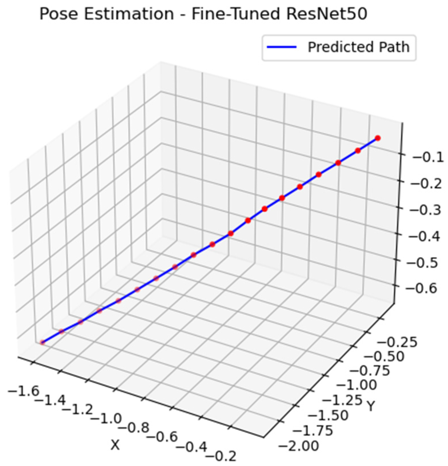The weights of the model are updated using the Adam optimizer (learning rate 1 × 10⁻⁴). MSE and MAE are determined as the loss function and the performance metric. During training, transformations (rotation, zoom, displacement, brightness change, and horizontal flip) are added to each image in the dataset by applying data augmentation. This process allows the model to learn on more data and reduces the risk of overfitting. The images are divided into 80% training and 20% validation with train–validation split. The batch size value used for training is 8, meaning that learning is performed on eight images at a time. In addition, early stopping is used to prevent the model from over-learning; here, if the validation loss does not improve for five epochs, the training is stopped. A total of 20 epochs are used during training, but early stopping can shorten the training time. The best model weights obtained in training are saved as the weights of the model with the lowest validation loss. Pseudo-pose data corresponding to each image was created with 0.5 cm increments only in the Z axis. As a result, the estimated positions were visualized with a three-dimensional graph, and the movement path followed by the model over time was drawn. The localization result of fine-tuned Resnet-50 is shown in Figure 14.

Figure 15 demonstrates the train and validation loss and MAE values of ResNet-50 implementation.

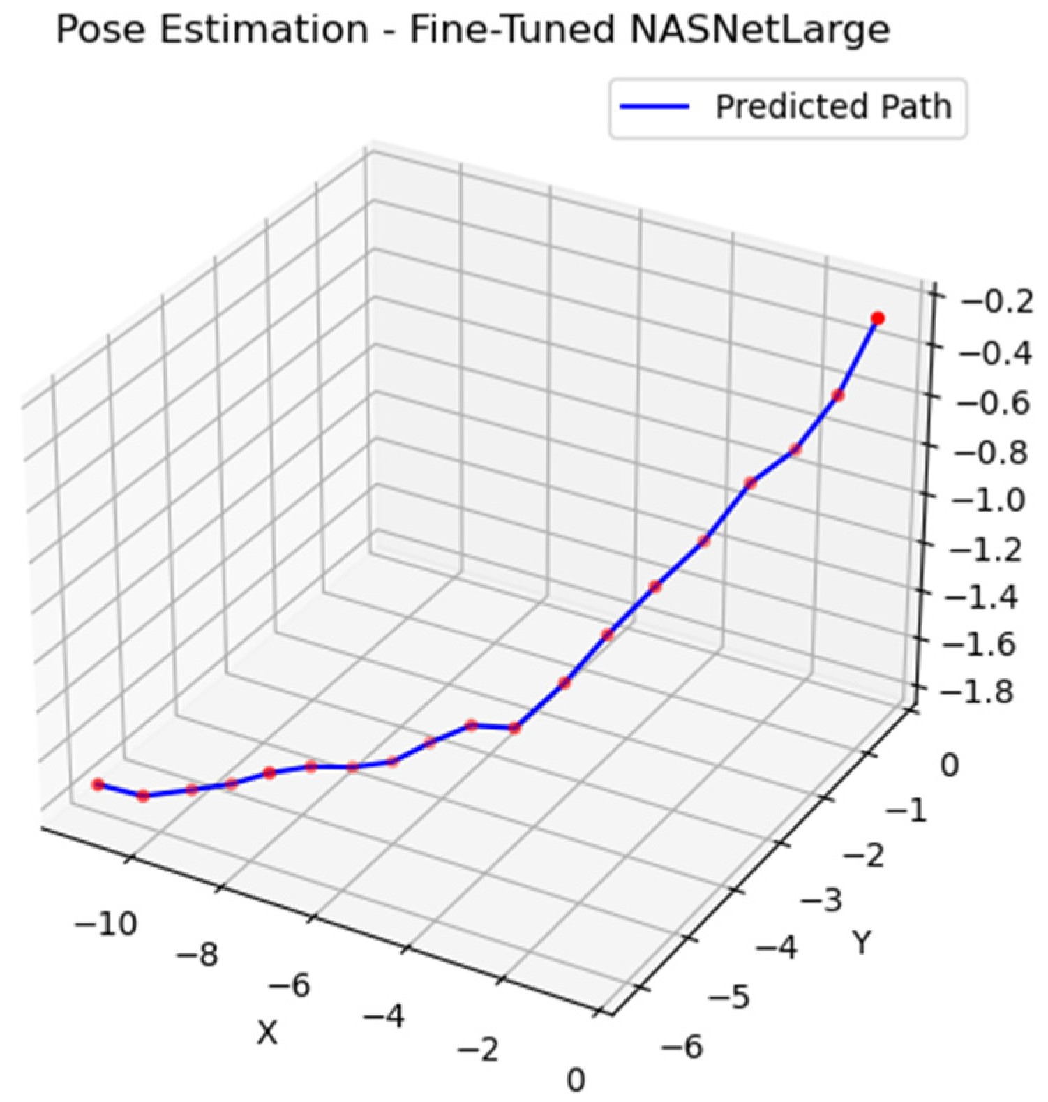
Finally, the NASNetLarge model pretrained on ImageNet was used for 6-DoF pose estimation from monocular endoscopic images. The implementation also includes data augmentation techniques such as image rotation, shift, and translation, thus increasing the training dataset from 19 original test images to 190 augmented images. The training process is performed by freezing the initial layers of the NASNetLarge model (to preserve the previously learned features) and training only the last 30 layers with the newly added regression head. The model is compiled with Adam optimizer and MSE loss. Consecutive endoscopic images used as input were resized and normalized to fit the model, and pseudo-pose labels created with only 0.5 cm increments along the Z axis were used for each image. The model was trained with a batch size of 8 for 20 epochs, and the total training time was measured and reported. After training, pose estimation was made for each image; the first position was accepted as the starting position, and the subsequent estimations were cumulatively collected to create a 3D tracking route. The obtained results were visualized in a 3D environment, and the motion estimation performance of the model was analyzed. The localization result of NASNetLarge is shown in Figure 16.

Figure 17 demonstrates the training and validation loss and MAE values of the NASNetLarge implementation.

The basic structures and training strategies of four different DL-based models used for 6-DoF pose estimation using monocular endoscopic images are shown in

Table 1. Architectural configurations and training parameters of the DL-based models.

Parameter	ResNet-50 (Fine-Tuned)	NASNetLarge (Fine-Tuned)	ResNet-50 (Fine-Tuned) + Farneback Optical Flow (Hybrid) and ResNet-50 (Fine-Tuned) + Lucas–Kanade Optical Flow
Backbone	ResNet-50	NASNetLarge	ResNet-50
Pretrained Weights	ImageNet	ImageNet	ImageNet
Trainable Layers	Last 30 layers + regression head	Last 30 layers + regression head	Last 30 layers + regression head
Epochs	20	20	20
Batch Size	8	8	8
Optimizer	Adam	Adam	Adam
Learning Rate	1 × 10−4	1 × 10−4	1 × 10−4
Loss Function	MSE	MSE	MSE
Pose Estimation Method	CNN-only (cumulative)	CNN-only (cumulative)	CNN + Optical Flow (weighted)
Dataset	Monocular endoscopic test area images	Monocular endoscopic test area images	Monocular endoscopic test area images

. The first two models are based on only CNN-based regression approach, using ResNet-50 and NASNetLarge backbones. The third and fourth model offers a hybrid pose estimation approach by considering the motion information between consecutive frames with the optical flow in addition to the classical CNN approach.

5. Results and Discussion

Each model was evaluated according to four different metrics: localization accuracy (RMSE), rotational accuracy, training time, and inference time per image, in the study.

A scale factor was assigned in order to obtain the real-world distances using Equations (22) and (23):

$$\mathrm{S}\mathrm{c}\mathrm{a}\mathrm{l}\mathrm{e} \mathrm{F}\mathrm{a}\mathrm{c}\mathrm{t}\mathrm{o}\mathrm{r}={\displaystyle \frac{\mathrm{R}\mathrm{e}\mathrm{a}\mathrm{l} \mathrm{D}\mathrm{i}\mathrm{s}\mathrm{t}\mathrm{a}\mathrm{n}\mathrm{c}\mathrm{e}}{\mathrm{M}\mathrm{o}\mathrm{d}\mathrm{e}\mathrm{l} \mathrm{D}\mathrm{i}\mathrm{s}\mathrm{t}\mathrm{a}\mathrm{n}\mathrm{c}\mathrm{e}}}$$

(22)

$$\mathrm{P}\left(\mathrm{s}\mathrm{c}\mathrm{a}\mathrm{l}\mathrm{e}\mathrm{d}\right)=\mathrm{P}\left(\mathrm{o}\mathrm{r}\mathrm{i}\mathrm{g}\mathrm{i}\mathrm{n}\mathrm{a}\mathrm{l}\right)\ast \mathrm{S}\mathrm{c}\mathrm{a}\mathrm{l}\mathrm{e} \mathrm{F}\mathrm{a}\mathrm{c}\mathrm{t}\mathrm{o}\mathrm{r}$$

(23)

RMSE calculation was carried out based on the real-world measurements between the image acquisition points, which is 0.5 cm between each point. Residuals (V) were obtained by calculating the differences between the values predicted by the model and the ground truth values. RMSE was calculated using these residuals.

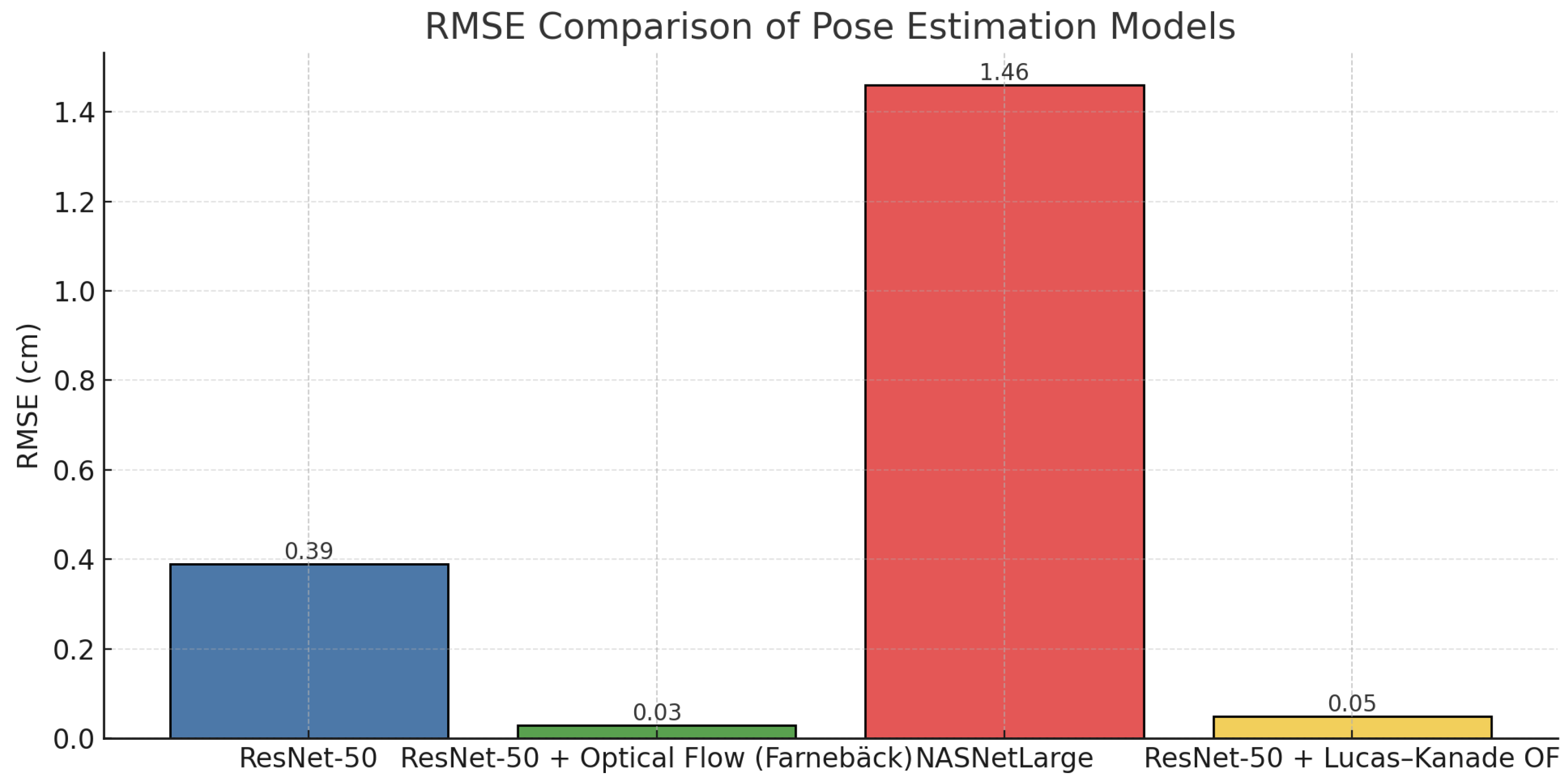
The fine-tuned ResNet-50 model showed a great performance in terms of RMSE, but the inference time was long. The NASNetLarge model achieved lower accuracy; the training and inference time were also very long. The proposed model in the study, ResNet-50–optical flow hybrid framework, outperformed its alternatives in accuracy and speed: it provided low RMSE and was reasonably fast. These results show that combining the motion information between consecutive frames with optical flow and the high-level visual features obtained with CNNs significantly improves pose estimation accuracy, especially in monocular camera localization tasks. RMSE comparison of pose estimation models is given in Figure 18.

The effect of the CNN weight (α) was also calculated in terms of RMSE (Figure 19).

As α increases (CNN weight increases), the RMSE decreases monotonously from 1.02 cm to 0.03 cm, indicating that the dominance of the CNN contribution in the hybrid significantly increases the accuracy, and the best result is obtained at α = 0.9.

Table 2. Comparison of different CNN-based models for monocular pose estimation in terms of RMSE, training time, and average inference time per frame.

Model	RMSE (cm)	Training Time (s)	Inference Time (ms/Frame)
ResNet-50	0.39	373.75	316.57
ResNet-50 (Fine-Tuned) + Farneback Optical Flow (Hybrid)	0.03	393.11	241.84
ResNet-50 (Fine-Tuned) + Lucas–Kanade Optical Flow	0.05	419.63	286.34
NASNetLarge	1.46	876.54	529.66

presents the comparative performances of different CNN-based models on the monocular pose estimation task.

The rotational accuracy was also tested. Images were taken on a flat surface on a fixed platform, and rotations were assumed as (0, 0, 0) for all test data. Rotation errors estimated by the ResNet-50 model remained at very low levels with roll (0.01 radian), pitch (0.02 radian), and yaw (0.05 radian) angles, indicating that the model provides accurate results in pose estimation. In the ResNet-50 (Fine-Tuned) + Farneback optical flow (Hybrid) model, more stable estimations were made, and rotation errors were further reduced thanks to the integration of optical flow. Roll (0.04 radian), pitch (0.013 radian), and yaw (0.015 radian) errors of this model reveal that optical flow increases accuracy with visual motion information. On the other hand, rotation errors are higher in NASNetLarge model; roll (0.14 radian), pitch (0.13 radian), and yaw (0.08 radian) errors show that the larger structure of the model causes a loss of accuracy when generalizing. Rotation errors estimated by the ResNet-50 (Fine-Tuned) + Lucas–Kanade optical flow was also noted as roll (0.09 radian), pitch (0.04 radian), and yaw (0.011 radian). In general, the combination of ResNet-50 and ResNet-50 (Fine-Tuned) + Farneback optical flow provided more accurate and reliable predictions in the tests performed on flat ground, showing that optical flow integration is beneficial. The rotational errors of each model are shown in

Table 3. The rotational errors of the models in roll, pitch, and yaw.

Model	Roll (Radian)	Pitch (Radian)	Yaw (Radian)
ResNet-50	0.01	0.02	0.05
ResNet-50 (Fine-Tuned) + Farneback Optical Flow (Hybrid)	0.04	0.013	0.015
ResNet-50 (Fine-Tuned) Lucas–Kanade Optical Flow	0.09	0.04	0.011
NASNetLarge	0.14	0.13	0.08

.

Classical feature-based methods, ORB and SIFT, were also evaluated for comparison. However, both methods suffered from significant tracking losses in the phantom environment. Especially in low-texture regions, the algorithms frequently failed because a sufficient number of reliable matches was not found, thus preventing a continuous trajectory. Therefore, RMSE calculation was not possible. This significant failure of ORB and SIFT demonstrates the limited applicability of classical methods to homogeneous tissues like intestines. In contrast, the proposed hybrid CNN + optical flow approach achieved stable localization throughout the entire sequence without any tracking loss in any frame and demonstrated superior performance with an error value of 0.03 cm. This clear contrast strongly demonstrates that the proposed method is much more reliable and robust than classical methods.

In the study, a new hybrid framework is proposed for 6-DoF pose estimation performed with monocular images in difficult and narrow areas such as CE. This framework evaluates both visual and temporal information simultaneously by combining a DL-based CNN model (fine-tuned ResNet-50) and the Farneback optical flow algorithm. The developed system aims to make the pose estimation task more accurate and stable by taking advantage of the continuity of motion between frames. The proposed framework in the study was tested comparatively with two different DL architectures. In addition, V-SLAM methods widely used in the existing literature were also applied in the test environment, but it was observed that SLAM algorithms could not provide sufficient accuracy and stability in this special scenario. Especially in endoscopic images with no texture, repeated patterns, and low distinctiveness, SLAM-based solutions experienced serious performance loss. The proposed system aims to increase both accuracy and stability in pose estimation by combining the deep visual feature extraction power of a fine-tuned ResNet-50 model with the temporal motion sensitivity of the Farneback optical flow algorithm. In the comparative experiments, the RMSE value of 0.39 cm in the ResNet-50 model was reduced to 0.03 cm in the hybrid model. The NASNetLarge model achieved lower success with 1.46 cm RMSE and also fell short in terms of inference time (529.66 ms/frame). In contrast, the proposed hybrid model showed the best performance with 0.03 cm RMSE and 241.84 ms/frame inference time; it provided an improvement of approximately 92.31% in terms of accuracy compared to the only CNN model. The results show that the proposed CNN + optical flow hybrid approach provides a reliable alternative, especially in challenging environments where SLAM fails. Thanks to its real-time operability and low error rate, this system is a candidate to be used as an effective pose estimation tool in medical imaging systems and CE applications. In our comparison, the Lucas–Kanade method provided competitive accuracy within our hybrid framework (e.g., RMSE = 0.05 cm for α = 0.9). However, a higher deviation was observed compared to the Farnebäck method (Farnebäck: 0.03 cm). Based on these findings, Farnebäck was chosen as the default flow component in this study; however, Lucas–Kanade offers value as a viable alternative.

We acknowledge that dense optical flow may produce unreliable vectors in low-texture regions. In our design, optical flow contributes only to short-term lateral refinements (x, y), while the CNN provides stable depth (z) and orientation. Thus, the fusion mitigates the weaknesses of each component. Furthermore, although the CNN is treated as a regressor, it effectively learns gradient- and texture-based cues relevant to intestinal structures. Future work will integrate geometric constraints or attention mechanisms to improve interpretability. From a clinical perspective, the localization accuracy achieved of 0.03 cm is quite promising. Current localization methods used in capsule endoscopy (e.g., magnetic tracking or RF-based techniques) typically provide accuracies on the order of a few millimeters. In contrast, our hybrid CNN + optical flow approach demonstrated submillimeter accuracy in a phantom environment, exceeding the requirements of current clinical standards. Although obtained in a phantom environment, these results demonstrate a proof-of-concept with submillimeter accuracy, highlighting the potential for improving patient outcomes in capsule endoscopy. Such accuracy could enable more reliable lesion localization, facilitate evaluation of intestinal motility and transit times, and support targeted therapeutic interventions. While the findings were achieved under controlled conditions, they indicate the applicability of the proposed framework and its potential clinical value once validated on larger and more diverse datasets. Future studies will focus on verifying whether this performance can be maintained in real-world patient data and across different tissue conditions of the gastrointestinal tract.

Limitations and Future Work

This study has several limitations. First, the dataset is relatively small, consisting of 19 original images acquired in a phantom environment; these images were expanded to 190 samples using data augmentation methods. While data augmentation increases diversity, a dataset of this size does not fully guarantee robust generalization of the model. Therefore, future studies will focus on collecting datasets that include a wider range of conditions and include data from real patients. Second, the phantom used in this study was designed primarily to mimic the jejunum segment, which has relatively homogeneous tissues. Therefore, the results obtained may not be directly generalizable to intestinal segments such as the duodenum and ileum, which exhibit different textures and contrast characteristics. Furthermore, the fusion strategy was implemented using a fixed α value (0.9), and while this value provided the best performance in our setup, its stability across different anatomical conditions has not yet been verified. Frame-to-frame accumulation inevitably causes drift over long trajectories. In our phantom setup, which involves short and controlled sequences, drift remained bounded. Future studies will incorporate loop closure and depth cues to mitigate long-term divergence and will aim to develop adaptive or dynamic fusion strategies to improve generalizability. This phantom study does not include bowel turns calibration strategies for curved segments, and patient-specific anatomy will also be addressed in future work.

6. Conclusions

This study focuses on the problem of providing accurate localization in challenging environments such as the small bowel, where feature-based SLAM approaches fail. For this purpose, a test area that mimics the human small bowel was created in the Opto-Electronics Laboratory. Therefore, a hybrid framework that combines ResNet-50 and optical flow is proposed and compared with different DL-based models and SLAM results.

The experiments show that training the entire ResNet-50 architecture with fine-tuning gives moderate pose estimation accuracy. However, the most successful results are obtained with the proposed hybrid model; this model provided the lowest error rate with an RMSE value of 0.03 cm. This situation demonstrates the effectiveness of DL models based on visual features to gain motion awareness with optical flow.

The findings show that hybrid localization approaches provide more stable and high-accuracy results, especially in visually challenging conditions such as gastrointestinal images. In future work, the aim is to further increase the localization performance in complex and dynamic environments by enriching this framework with inertial measurement units (IMU) and evaluating transformer-based architectures. The original aspects and scientific contributions of the study are presented below:

A localization framework has been developed to address the failures of V-SLAM algorithms, tested in small-intestine-like conditions.

A hybrid method combining DL-based CNN architecture with optical flow information has been proposed.

This hybrid approach provides more stable and reliable pose estimation in visually homogeneous, low-contrast, and repetitive patterned environments.

The success of the hybrid model was evaluated comparatively with different DL architectures and classical SLAM methods, and it was revealed that the proposed approach was superior in terms of both accuracy and stability.

In areas where traditional methods failed, frame-based error accumulation was reduced by using optical-flow-based motion information, and pose estimation was made more consistent.

The study proposes a reliable and extensible solution for clinical applications such as CE.

Future studies aim to test the method with real patient data, add rotational motion components to the optical flow algorithm, and make the system real-time with hardware acceleration.