Differentiable Selection of Bit-Width and Numeric Format for FPGA-Efficient Deep Networks

Abstract

Quantization-aware training (QAT) has emerged as a key strategy for enabling efficient deep learning inference on resource-constrained platforms. Yet, most existing approaches rely on static, manually selected numeric formats—fixed-point or floating-point—and fixed bit-widths, limiting their adaptability and often requiring extensive design effort or architecture search. In this work, we introduce a novel QAT framework that breaks this rigidity by jointly learning, during training, both the numeric representation format and the associated bit-widths in an end-to-end differentiable manner. At the core of our method lies a unified parameterization that is capable of emulating both fixed- and floating-point arithmetic, paired with a bit-aware loss function that penalizes excessive precision in a hardware-aligned fashion. We demonstrate that our approach achieves state-of-the-art trade-offs between accuracy and compression on MNIST, CIFAR-10, and CIFAR-100, reducing average bit-widths to as low as 1.4 with minimal accuracy loss. Furthermore, FPGA implementation using Xilinx FINN confirms over $5\times$ LUT and $4\times$ BRAM savings. This is the first QAT method to unify numeric format learning with differentiable precision control, enabling highly deployable, precision-adaptive deep neural networks.

1. Introduction

Convolutional Neural Networks (CNNs) have become foundational to modern computer vision, powering tasks such as image classification, object detection, and semantic segmentation [1,2]. These achievements, however, rely heavily on the computational power of GPUs and large-scale cloud infrastructure. As deep learning expands into the real world, latency-sensitive, and power-constrained applications—such as autonomous vehicles, wearable devices, and edge AI—these resource-intensive architectures face growing deployment challenges [3,4]. High memory requirements and compute demands make them ill-suited for constrained environments.

Field-Programmable Gate Arrays (FPGAs) have emerged as a promising platform for energy-efficient inference due to their reconfigurable logic, fine-grained parallelism, and low-latency execution [5,6]. Still, efficient deployment of CNNs on FPGAs requires careful co-optimization of arithmetic precision and memory hierarchy.

In this work, we target the Pynq-Z2 FPGA board, which features a Xilinx Zynq-7000 SoC with 53,200 LUTs, 140 Block RAM (BRAM) units, and 220 DSP slices, providing a concrete constraint context for evaluating the memory and arithmetic efficiency of CNN deployment.

While it is well established that floating-point arithmetic consumes more LUTs, FFs, and DSP slices than fixed-point [7] arithmetic, recent studies emphasize that the dominant cost in FPGA accelerators is often not arithmetic resources themselves but memory movement. Data transfers from off-chip DRAM can be one to two orders of magnitude more energy intensive than a multiply–accumulate (MAC) operation [8,9], meaning that the overall number of bits shuttled through the memory hierarchy frequently outweighs the choice of operator type in determining system-level efficiency. This has led to a shift in quantization research from purely minimizing logic cost to more holistic strategies that reduce precision where possible and preserve it where necessary to avoid excessive memory overhead  [5,10].

Precision trade-offs therefore require careful consideration. Lower bit-widths reduce storage and memory access energy but may compromise accuracy; higher precision improves robustness but increases both computational and memory footprints. Full-precision (32-bit floating-point) models are clearly mismatched to FPGA deployment. However, uniform fixed-point quantization may also be suboptimal, as it lacks the dynamic range required in certain layers and can force over-provisioning of bit-widths [11,12]. In such cases, compact floating-point representations with a few exponent bits can achieve comparable or better efficiency by lowering the average precision across the network while retaining range where needed. This balance directly impacts both accuracy and energy consumption, particularly in memory-bound workloads.

To address this challenge, we propose a quantization-aware training (QAT) framework that adapts both the arithmetic mode (fixed-point or floating-point) and the associated bit-widths at the layer level. Unlike prior approaches that impose a uniform representation [12,13] or rely on costly multi-path neural architecture search [3,14], our method treats exponent and mantissa widths as continuous, differentiable parameters optimized end-to-end during training. This enables the network to automatically discover hybrid configurations where fixed-point suffices in most layers while low-precision floating-point is selectively used to capture dynamic range with minimal bit cost. As a result, the framework reduces memory access volume—the true bottleneck of FPGA accelerators—while maintaining accuracy and ensuring a hardware-friendly static configuration at inference.

• Our main contributions are as follows:

1.

We introduce a unified numerical format that can seamlessly interpolate between fixed-point and floating-point behavior, with exponent and mantissa precision learned during training.

2.

We develop a fully differentiable, single-path QAT framework that avoids multi-path overhead and enables scalable deployment.

3.

We demonstrate that hybrid quantization discovered by our framework reduces overall memory traffic and improves hardware efficiency, highlighting that resource trade-offs in FPGA deployment must be assessed holistically rather than solely by arithmetic operator cost.

2. Related Work

Quantization of deep neural networks (DNNs) has emerged as a critical strategy for enabling the efficient deployment of AI models on edge devices and specialized hardware platforms such as FPGAs and ASICs. In this section, we review prior work in quantization-aware training (QAT), mixed-precision methods, and learnable numerical formats, highlighting how our contribution builds upon and extends these foundations.

2.1. Quantization-Aware Training (QAT)

Quantization-aware training simulates low-precision arithmetic during training, enabling models to adapt their weights and activations to the effects of quantization noise. Pioneering works such as DoReFa-Net [12] and Binarized Neural Networks (BNNs) [13,15] demonstrated the feasibility of extreme quantization (e.g., 1-bit) while retaining acceptable accuracy. However, these methods rely on fixed precision levels and static configurations, often determined heuristically.

More recent approaches such as QAT in TensorFlow [11] and Brevitas [16] enable broader support for low-bit quantization (e.g., 2–8 bits), but remain limited to fixed-point formats with hand-crafted bit-width settings. These systems often do not optimize precision during training, leading to suboptimal trade-offs between model performance and hardware efficiency.

Building on these foundations, the latest research has begun to explore hybrid and adaptive quantization strategies that extend beyond fixed-point arithmetic. For example, AdaQuant-FP [10] introduced an adaptive floating-point scheme that dynamically allocates exponent and mantissa bits to minimize memory traffic while preserving range, showing benefits in FPGA deployment. Similarly, quantization methods for transformers have emerged, where mixed-precision strategies are selectively applied to attention layers and feed-forward blocks [17]. These studies reflect a broader trend toward hybrid representations, balancing dynamic range and precision to improve both efficiency and accuracy. Our work differs by unifying fixed-point and floating-point behavior within a single differentiable framework, enabling end-to-end learning of bit-widths and formats without the need for manual exploration or task-specific heuristics.

2.2. Mixed-Precision and Bit-Width Optimization

Mixed-precision quantization assigns different bit-widths to different layers or tensors to better balance accuracy and computational cost. HAWQ [18] and its successors (HAWQ-V2/V3) introduced Hessian-based sensitivity metrics to guide bit allocation, achieving strong results under hardware constraints. Similarly, LQ-Nets [19] employed learnable quantizers but required discretization steps and specialized search procedures.

AdaQuant and AdaQAT [10,20] proposed gradient-based fine-tuning of quantized models with adaptive bit-widths, showing improved trade-offs between accuracy and latency. However, these methods often depend on offline pre-trained models and require separate bit allocation stages, limiting their adaptability.

In contrast, our method integrates bit-width learning into the training loop, enabling end-to-end optimization of both model weights and numerical precision. Unlike previous methods, our bit-widths are differentiable parameters, optimized dynamically via backpropagation, and applicable to both floating-point and fixed-point domains through a unified formulation.

2.3. Learnable Numeric Formats

Recent research has explored learning the numerical format itself. HATO [21] introduced hierarchical token-based quantization for transformers, while Q-BERT [22] used reinforcement learning for precision assignment. Other works such as FQ-ViT [23] extend quantization to vision transformers with per-layer and per-token bit-widths.

Our method builds upon these ideas by introducing a learnable numerical representation $\tilde{F}$ that includes mantissa, exponent, and scale parameters, thus supporting both fixed- and floating-point semantics. This flexibility enables our system to choose the most hardware-appropriate format per layer, while previous works are often restricted to one format.

2.4. Hardware-Aware Optimization and Deployment

Hardware-aware neural architecture search (HW-NAS) [3,24] and inference-aware training [14] have emphasized the importance of incorporating hardware costs into training objectives. Yet, most HW-NAS approaches are computationally expensive due to architecture sampling and model duplication.

In contrast, our framework operates via single-path training, avoiding layer replication and providing fine-grained numerical control. We integrate the bit penalty directly into the loss, which acts as a soft regularization toward hardware efficiency. Moreover, our method is deployable on real FPGAs using tools such as FINN [5], where it demonstrates tangible resource savings.

Our work offers a significant advancement over prior quantization methods by proposing a novel training paradigm that is both algorithmically adaptive and hardware-aware. Unlike earlier approaches that treat precision levels as static or search-based hyperparameters, our method learns bit-widths dynamically via gradient descent, enabling fully end-to-end optimization. Furthermore, by unifying floating-point and fixed-point arithmetic within a single differentiable quantization framework, we allow the model to flexibly adjust its numeric representation based on the computational needs of each layer.

The integration of a differentiable bit-aware loss function further distinguishes our approach, as it enforces hardware-aligned constraints during training without relying on post hoc quantization steps. This leads to better utilization of bit budgets and finer control over performance–efficiency trade-offs. Finally, our method supports seamless deployment on FPGA hardware, where our layer-wise precision adaptation translates directly into measurable reductions in resource utilization—offering practical benefits in real-world embedded systems.

3. Theoretical Framework

3.1. Numerical Representations in Hardware

Neural networks are traditionally trained using 32-bit floating-point numbers, which offer high precision but require significant computational and memory resources. These constraints make such models unsuitable for deployment on hardware with limited resources, such as FPGAs and embedded systems. To enable efficient inference, reduced-precision formats—such as fixed-point and low-bit-width floating-point representations (e.g., 16-bit or 8-bit)—have gained popularity.

In general, any numeric computation on hardware involves mapping continuous real-valued tensors $T\in {\mathbb{R}}^n$ into a discrete, hardware-supported format. The efficiency of this representation depends on how bits are allocated to encode numerical values—whether it is through explicit fields (e.g., sign, exponent, and mantissa in floating-point formats) or implicit encoding schemes (e.g., two’s complement in fixed-point representations).

3.2. Floating-Point Representation

The most common numerical format is the floating-point representation:

$$\mathrm{FP}=\{s,e,m\}$$

The number is stored as a sequence of bits divided into sign (1 bit), exponent (8 bits), and mantissa (23 bits).

$$\underset{\mathrm{Sign} \left(1\mathrm{bit}\right)}{\underbrace{\phantom{(}1}}\underset{\mathrm{Exponent} \left(b_e=8\right)}{\underbrace{\phantom{(}{\displaystyle 10000110}}}\underset{\mathrm{Mantissa} \left(b_m=23\right)}{\underbrace{\phantom{(}{\displaystyle 1001101000111100010101}}}$$

$$\mathrm{FP}=\{s,e,m\},\mathrm{where}s\in \{0,1\}\left(\mathrm{sign}\right),e\in \{0,\dots ,2^{b_e}-1\}\left(\mathrm{exponent}\right),m\in \{0,\dots ,2^{b_m}-1\}\left(\mathrm{mantissa}\right)$$

The corresponding real number is reconstructed as follows:

$$F={(-1)}^s·\left(1+{\displaystyle \frac{m}{2^{b_m}}}\right)·2^{e-2^{b_e-1}}$$

(1)

3.3. Fixed-Point Representation

In contrast, the fixed-point representation avoids the complexity of an exponent field by assuming a fixed scaling factor:

$$\mathrm{FXP}=\{m,d\}$$

where $m\in \{-2^{b_m-1},\dots ,2^{b_m-1}-1\}$ is a signed integer, and $d\in \mathbb{Z}$ is a constant scaling exponent. Its real-valued interpretation is as follows:

$$F=m·2^d$$

(2)

Fixed-point is computationally efficient and hardware-friendly but lacks flexibility in handling large or small magnitudes in a single model.

3.4. Our Learnable Numeric Format

To enable each layer to autonomously choose the most suitable numerical format, we introduce a unified, learnable representation that is capable of expressing both fixed-point and floating-point arithmetic:

$$\tilde{F}=\{s,m,e,d\}$$

with:

• s: sign bit;
• m: mantissa (with learnable bit-width $b_m$);
• e: exponent (with learnable bit-width $b_e$);
• d: per-layer scale factor.

The mapping to real numbers is defined as follows:

$$\tilde{F}={(-1)}^s·\left(1+{\displaystyle \frac{m}{2^{b_m}}}\right)·2^{e-2^{b_e-1}+d}$$

(3)

This representation allows the model to learn, during training, whether a given layer should behave more like fixed-point (via d) or floating-point (via e), without requiring duplicated or separate architectures.

3.5. Learning Arithmetic Behavior During Training

The key innovation is that our format can dynamically emulate either fixed-point or floating-point arithmetic based on learned parameters:

• Fixed-point behavior: If the model sets $b_e=0$ (i.e., no exponent), the format simplifies to the following equation:

  $${\tilde{F}}_{\mathrm{fixed}}={(-1)}^s·\left(1+{\displaystyle \frac{m}{2^{b_m}}}\right)·2^d$$
  When $b_e\to 0$, the exponent field vanishes, yielding a purely scaled integer format.
• Floating-point behavior: If the model sets $d=0$, we recover a floating-point format:

  $${\tilde{F}}_{\mathrm{float}}={(-1)}^s·\left(1+{\displaystyle \frac{m}{2^{b_m}}}\right)·2^{e-2^{b_e-1}}$$
  When $d\to 0$, the format reduces to classical floating-point representation with bias-corrected exponent scaling.
• Hybrid Regime: When both $b_e$ and d are nonzero, we obtain a numerically stable mixed-format that is ideal for non-stationary activations.

The model automatically learns whether to emphasize dynamic scaling (via exponent) or static precision (via scaling factor d), depending on the sensitivity of each layer to quantization.

This hybrid approach allows the following:

• Layer-wise precision tuning: Each layer can choose the most efficient format based on its computational role.
• Gradient-based optimization: Unlike traditional methods that discretely search architectures, we optimize bit-width and arithmetic behavior jointly via backpropagation.
• Hardware portability: This design maps naturally onto both fixed-function hardware (e.g., ASICs) and configurable platforms (e.g., FPGAs).

This unified formulation underpins the precision-aware training pipeline and supports efficient, accurate deployment on resource-constrained hardware.

We summarize all symbols introduced in Section 3 in

Table 1. Summary of symbols used in Section 3.

Symbol	Definition
s	Sign bit ($s\in \{0,1\}$)
m	Mantissa value (integer-encoded fraction)
$b_m$	Bit-width of the mantissa (learnable)
e	Exponent value
$b_e$	Bit-width of the exponent (learnable)
d	Per-layer scaling factor (fixed integer shift)
$\tilde{F}$	Learned unified numeric format
F	Real-valued reconstruction of a number
T	Input tensor $T\in {\mathbb{R}}^n$

.

4. Materials and Methods

4.1. Overview

This work proposes a novel single-path quantization-aware training framework integrated with a flexible numerical format. The framework enables each neural network layer to dynamically select between fixed-point and floating-point quantization formats and to learn the optimal bit-widths for exponent and mantissa during training. This approach eliminates the need for duplicating layers or models, reducing computational overhead while optimizing both accuracy and hardware efficiency.

4.2. Quantization Wrappers

To enable flexible quantization, we introduce two wrapper modules applied to each network layer:

• QuantWrapperFloatingPoint: This wrapper models a floating-point quantization scheme where the bit-widths of the exponent ($e\_bits$) and mantissa ($m\_bits$) are learnable parameters. These parameters are initialized as trainable tensors (nn.Parameter) allowing gradient-based optimization. The wrapper applies quantization to both weights and activations by simulating the reduced-precision floating-point arithmetic during the forward pass.
• QuantWrapperFixedPoint: This wrapper implements fixed-point quantization with predefined bit-widths. Unlike the floating-point wrapper, the bit-widths are fixed and non-learnable. This wrapper provides a baseline quantization scheme for comparison and hybrid usage.

Both wrappers share a common interface including methods for quantization and extraction of current bit-widths, facilitating their interchangeable use in the model.

4.3. Model Architecture and Single-Path Training

The quantization wrappers are integrated into the base model architecture by replacing standard layers with their quantized counterparts wrapped by either QuantWrapperFloating Point or QuantWrapperFixedPoint. The choice of quantization wrapper defines the numerical format for the entire network during training.

This design supports a single-path training scheme, where only one unified model instance is maintained throughout training and inference. By avoiding layer or model duplication, the framework significantly reduces memory consumption and simplifies the training pipeline.

4.4. Bit-Aware Loss Function: Learnable Bit-Width Optimization

A central contribution of our framework is the formulation of a bit-aware loss function, which enables the model to learn not only task performance but also its own numeric precision configuration. This is achieved by integrating a differentiable penalty term into the training objective that discourages high bit-width usage across the network. The resulting loss function is expressed as follows:

$${\mathcal{L}}_{\mathrm{total}}={\mathcal{L}}_{\mathrm{task}}(y,\widehat{y})+\lambda \sum _{l=1}^L\left(b_e^{\left(l\right)}+b_m^{\left(l\right)}\right),$$

(4)

where ${\mathcal{L}}_{\mathrm{task}}(y,\widehat{y})$ is the task-specific loss (e.g., cross-entropy for classification), and $b_e^{\left(l\right)}$ and $b_m^{\left(l\right)}$ represent the learned exponent and mantissa bit-widths for layer l, respectively. The hyperparameter $\lambda$ governs the trade-off between numerical efficiency and task accuracy.

We further define a precision cost function for each layer l as follows:

$${\mathrm{BitCost}}^{\left(l\right)}=b_e^{\left(l\right)}+b_m^{\left(l\right)}=e^{p_e^{\left(l\right)}}+e^{p_m^{\left(l\right)}},$$

(5)

where $p_e^{\left(l\right)},p_m^{\left(l\right)}\in \mathbb{R}$ are log-domain parameters trained via gradient descent. This exponential reparameterization ensures the bit-widths remain strictly positive, differentiable, and smoothly optimized. Substituting this into Equation (4) yields a compact and expressive loss:

$${\mathcal{L}}_{\mathrm{total}}={\mathcal{L}}_{\mathrm{task}}+\lambda \sum _{l=1}^L{\mathrm{BitCost}}^{\left(l\right)}.$$

(6)

Crucially, our method enables learnable precision through direct gradient flow. The gradients of the total loss with respect to the bit-width parameters are analytically tractable:

$${\displaystyle \frac{\partial {\mathcal{L}}_{\mathrm{total}}}{\partial p_e^{\left(l\right)}}}=\lambda ·e^{p_e^{\left(l\right)}}=\lambda ·b_e^{\left(l\right)},{\displaystyle \frac{\partial {\mathcal{L}}_{\mathrm{total}}}{\partial p_m^{\left(l\right)}}}=\lambda ·b_m^{\left(l\right)},$$

(7)

demonstrating that the bit penalty behaves analogously to an $L_1$-like regularizer applied to bit-precision. These gradients guide the optimizer to reduce precision only where it least affects the task objective, enabling dynamic precision reallocation across layers.

The gradients in Equation (7) demonstrate how the bit penalty guides precision reduction where it least affects task performance. This optimization directly translates to hardware efficiency: in Section 5.9, we show that models trained with this loss achieve over 5× LUT and 4× BRAM savings on FPGAs, as the learned bit-widths minimize redundant logic and memory usage. The hyperparameter $\lambda$ thus serves as a tunable knob for accuracy–resource trade-offs, validated empirically in Figure 1 and later hardware experiments.

Figure 1 illustrates the trade-off enabled by our formulation. The bit-penalty coefficient $\lambda$ controls the trade-off between model accuracy and hardware efficiency. We determine $\lambda$ empirically through a validation set sweep, selecting values that maintain accuracy within 1% of the full-precision baseline while maximizing bit-width reduction. For small values of $\lambda$, the model behaves similarly to standard quantization-aware training (QAT), preserving accuracy with little pressure to reduce precision. As $\lambda$ increases, the optimizer is incentivized to shrink bit-widths, achieving significant compression at a graceful cost to accuracy. For example, increasing $\lambda$ from $0.01$ to $5.0$ leads to a drop in average bit-width from $10.4$ bits to just $1.5$ bits, with a negligible decline in classification performance.

This framework unlocks per-layer bit-width customization in a fully end-to-end fashion, where each layer discovers the optimal numeric representation—fixed-point or floating-point—suited to its computational role. Early convolutional layers often retain higher bit-widths due to their sensitivity, while deeper or fully connected layers tend to converge to minimal configurations.

From a hardware perspective, the penalty term can be interpreted as a proxy for energy or memory cost, with the total loss modeling an energy–accuracy trade-off:

$${\mathcal{L}}_{\mathrm{total}}={\mathcal{L}}_{\mathrm{task}}+\lambda ·{\mathcal{E}}_{\mathrm{precision}},$$

(8)

where ${\mathcal{E}}_{\mathrm{precision}}={\sum }_{l=1}^L{\mathrm{BitCost}}^{\left(l\right)}$ quantifies the model’s numerical footprint. This enables system-level co-optimization, where models are trained to meet both algorithmic and deployment constraints.

  In summary, the bit-aware loss function supports a gradient-friendly, hardware-efficient optimization paradigm that dynamically allocates numeric precision based on task complexity and resource constraints. It bridges the gap between quantization granularity and performance fidelity—empowering deployable deep learning at the edge.

4.5. Training Procedure

The training procedure follows these steps:

1.

Initialize the model with quantized layers wrapped by the chosen quantization wrapper.

2.

For each training batch, complete the following steps:

• Perform a forward pass applying simulated quantization with current bit-width parameters.
• Compute the combined loss incorporating both the task loss and the bit-width penalty.
• Backpropagate gradients to update model weights as well as bit-width parameters.
• Update model parameters using the optimizer.

3.

Periodically evaluate the model on a validation set to track accuracy and bit-width usage.

Additionally, learning rate scheduling is applied to facilitate stable convergence.

4.6. Datasets

For evaluation, we employed MNIST, CIFAR-10, and CIFAR-100, three widely used computer vision benchmarks. These datasets provide a progression of difficulty: MNIST (handwritten digits) is simple and enables the rapid validation of our framework; CIFAR-10 introduces natural images with moderate complexity; and CIFAR-100 further increases task difficulty by expanding the number of classes to 100, providing a stronger test of generalization. This selection ensures that our method is validated across datasets of increasing scale and granularity, allowing us to demonstrate both efficiency and accuracy trade-offs under varied conditions.

4.7. Evaluation and Model Selection

After training, models are evaluated on test datasets measuring both task accuracy and average bit-width usage. We save the following:

• The best accuracy model, maximizing task performance;
• The lowest bit-width model, minimizing quantization cost.

The learned bit-widths ($e\_bits$, $m\_bits$) for each quantized layer are extracted and can be rounded for hardware deployment. The final model parameters and quantization settings are exported for reproducibility and further analysis.

4.8. Implementation Details

The framework is implemented in PyTorch 1.13.1. The quantization wrappers extend torch.nn.Module and utilize torch.autograd.Function to define custom forward and backward passes for quantization and bit-width parameter updates.

The bit-width penalty terms are computed by aggregating learnable bit-width parameters across all quantized layers, normalized by the number of parameters.

The entire pipeline supports GPU acceleration and is compatible with standard datasets (e.g., CIFAR-10, MNIST).

This methodology enables a unified and flexible quantization-aware training framework that balances accuracy and hardware efficiency by learning optimal numerical formats on a per-layer basis without structural overhead.

4.9. Learnable Numerical Precision via Differentiable Floating-Point Truncation

At the core of our method lies a custom operation called FakeFloatFunction, which enables the differentiable quantization of numerical formats. This module simulates a floating-point, as shown in Figure 2 representation with learnable exponent and mantissa bit-widths, as well as a tunable scale factor. Unlike traditional fixed quantization schemes, our operator can adaptively learn which numerical format best suits each layer or tensor during training, bridging the divide between fixed-point, floating-point, and mixed formats.

4.9.1. Concept and Motivation

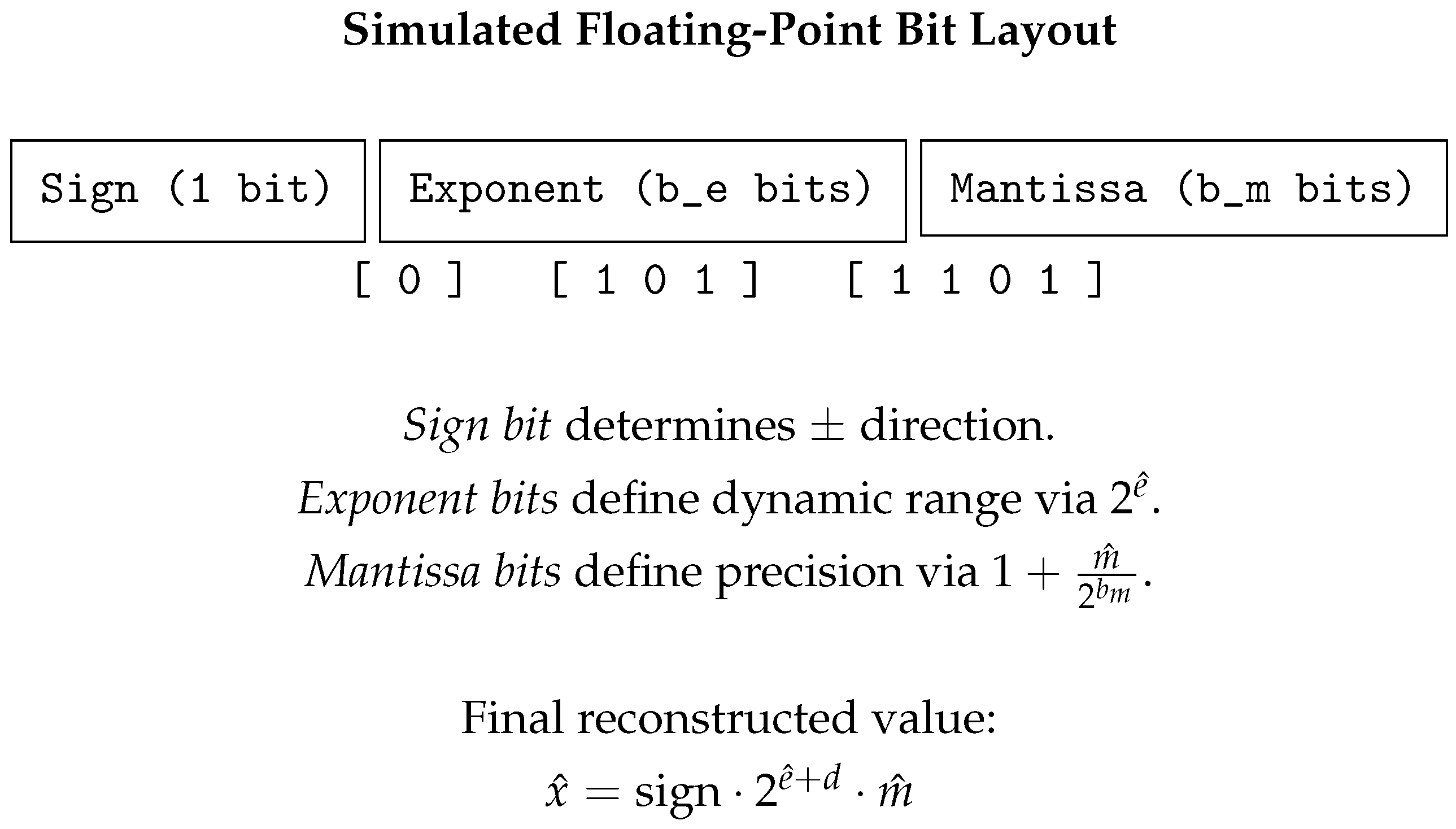
Floating-point representations in hardware are defined by three core components: sign, exponent, and mantissa, as illustrated in Figure 3. Most neural quantization schemes either fix these components (e.g., in IEEE-754 half or single precision) or discard the exponent entirely, opting for fixed-point arithmetic. However, this one-size-fits-all approach fails to capture the heterogeneous dynamic ranges across layers or even within feature maps. Our operator addresses this by enabling a fully customizable and learnable floating-point representation:

$$\mathtt{FakeFloat}\left(x\right)=\mathrm{sign}\left(x\right)·2^{\hat{e}}·\hat{m}·2^s$$

where $\hat{e}=Q(e;b_e)$, $\hat{m}=Q(m;b_m)$ (quantized via Equation (7)’s bit-truncation), and s is a learnable scale factor.

4.9.2. Forward Pass Mechanics

The forward pass, implemented in fake_float_truncate, proceeds as follows:

• The input tensor x is decomposed into sign, exponent, and mantissa via base-2 logarithms.
• The exponent is shifted and clamped to a learnable bit-width $e_{\mathrm{bits}}$, effectively simulating dynamic range control.
• The mantissa is truncated to $m_{\mathrm{bits}}$ bits by simple scaling and flooring.
• The tensor is reassembled using these quantized components and scaled back to the original range using a learnable scale parameter.

This operation mimics the arithmetic of hardware-level floating-point computation while maintaining differentiability with respect to format parameters.

4.9.3. Backward Pass with Differentiable Bit Control

To allow gradient-based learning of the format parameters $(e_{\mathrm{bits}},m_{\mathrm{bits}},s)$, we implement custom backward gradients via numerical approximation using central differences:

$${\displaystyle \frac{\partial \mathtt{FakeFloat}\left(x\right)}{\partial p}}\approx {\displaystyle \frac{-f(x+2h)+8f(x+h)-8f(x-h)+f(x-2h)}{12h}}$$

where p can be any of the learnable parameters. This allows us to propagate gradients to the number of bits used for the exponent and mantissa, despite their inherently discrete nature.

The bit-widths are stored as continuous parameters internally and are converted to integer values during the forward pass using a smooth transformation function (param_to_bit). This ensures compatibility with gradient descent optimizers while enforcing bit-width constraints during inference.

4.9.4. Unifying Fixed-Point and Floating-Point Formats

A particularly novel aspect of our formulation is that when $e_{\mathrm{bits}}=0$, the operator collapses to fixed-point arithmetic:

$$\mathtt{FakeFloat}\left(x\right)=\mathrm{sign}\left(x\right)·\widehat{m}·2^s$$

In contrast, when $e_{\mathrm{bits}}>0$, the representation becomes a true floating-point format. This duality makes it possible for the optimizer to select between fixed-point and floating-point behavior per tensor, offering an unprecedented level of format flexibility.

4.9.5. Practical Implications

This operator is plug-and-play within PyTorch training pipelines and does not require any external quantization framework. It supports deployment to FPGAs via learned parameters that can be exported to compatible formats in FINN or HLS4ML. The precision assignment becomes an outcome of training, not a design-time manual heuristic.

4.9.6. Mapping Bit Parameters via Param_to_Bit

To enable gradient-based optimization of bit-widths, we use a continuous parameterization. Internally, the number of bits for exponent and mantissa are represented as unconstrained real-valued parameters (e.g., $p_e,p_m$). These are mapped to discrete bit counts using a soft transformation function:

$$b=\mathtt{param}\_\mathtt{to}\_\mathtt{bit}\left(p\right)={log}_2\left(1+exp\left(p\right)\right)$$

This transformation ensures thathe following:

• Bit-widths remain positive ($b>0$);
• The function is smooth and differentiable for backpropagation;
• It behaves linearly for large values of p but avoids instability near zero.

• During the forward pass, the resulting bit-width b is rounded to the nearest integer:

$$b_{\mathrm{int}}=⌊\mathtt{param}\_\mathtt{to}\_\mathtt{bit}\left(p\right)+0.5⌋$$

This design preserves the discrete nature of bit allocation in deployment while allowing for optimization in continuous space during training.

4.10. Simulated Fixed-Point Quantization via Learnable Truncation

To emulate and learn quantization effects in a fixed-point numerical format during training, we introduce a custom differentiable function, FakeFixedFunction, which encapsulates a learnable, simulated fixed-point rounding scheme. This allows for gradient flow through bit-level quantization parameters such as bit-width, scaling, and zero-point bias.

4.10.1. Forward Truncation: Quantize and Dequantize

The forward pass simulates the quantization of a tensor $x\in \mathbb{R}$ into a fixed-point format using the following:

• $\mathtt{bits}\_\mathtt{int}$: total number of bits, b;
• $\mathtt{scale}\_\mathtt{int}$: scaling exponent, s;
• $\mathtt{zero}\_\mathtt{point}\_\mathtt{int}$: integer zero-point offset, $z_p$.

The quantized value is computed as follows:

$$q_x=\mathrm{clip}\left(⌊x·2^{s+\frac{b}{2}}+2^{b-1}+z_p⌉,0,2^b-1\right)$$

The quantized value is then dequantized back into floating-point format:

$$\hat{x}=\frac{q_x-2^{b-1}-z_p}{2^{s+\frac{b}{2}}}$$

This operation simulates symmetric signed fixed-point rounding and is implemented in the function fake_fixed_truncate().

4.10.2. Bit-Level Format Visualization

The simulated fixed-point format can be visualized as a fixed number of bits representing a centered quantization grid:

	[ MSB    …   LSB ]
	$\underset{b\mathrm{bits}}{\underbrace{0101\dots }}$
	$\Downarrow$
	$\mathrm{Integer}:q_x\in [0,2^b-1]$
	$\mathrm{Dequantized}:\widehat{x}={\displaystyle \frac{q_x-2^{b-1}-z_p}{2^{s+b/2}}}$

This illustrates how quantized values are symmetrically placed around zero after removing the zero-point and scale offsets.

4.10.3. Backward Pass: Learnable Quantization Parameters

The function FakeFixedFunction implements a differentiable proxy using a custom backward pass. Gradients are computed for all parameters using central difference approximations. For any parameter $p\in \{b,s,z_p\}$, the gradient is computed as follows:

$${\displaystyle \frac{\partial \widehat{x}}{\partial p}}\approx {\displaystyle \frac{-f(p+2h)+8f(p+h)-8f(p-h)+f(p-2h)}{12h}}$$

This fourth-order central difference estimator ensures stable and accurate gradients even with discrete bit-level steps.

4.10.4. Learnable Quantization via Param_to_Bit

To support the differentiability of the bit-width b, the integer-valued bits_int is derived from a continuous parameter using the param_to_bit() function, which maps a real-valued tensor to a positive integer using the following equation:

$$\mathtt{bits}\_\mathtt{int}=⌊{log}_2\left(1+exp\left(p\right)\right)⌉$$

This smooth mapping ensures that gradients can propagate through the bit parameter during training.

The simulated fixed-point truncation module described here provides a differentiable and learnable abstraction of hardware-friendly integer arithmetic. It enables the network to learn not only the weights and activations but also the optimal quantization configuration, which is essential for neural architecture search, quantization-aware training, and adaptive compression techniques.

The FakeFloatFunction lies at the heart of our adaptive quantization method. By unifying floating and fixed-point arithmetic in a differentiable framework and enabling bit-precision to be learned jointly with network parameters, it lays the groundwork for precision-aware neural architectures that can dynamically adapt to target hardware constraints during training.

5. Results

We evaluate our proposed precision-adaptive quantization framework across multiple datasets and compare its performance against baseline full-precision models and state-of-the-art quantization methods. All experiments are conducted using a VGG-inspired architecture [25], in alignment with prior work from FINN [26], enabling direct comparison.

5.1. Experimental Setup

The network architecture consists of three blocks of 2D convolution, batch normalization, and max pooling layers, followed by two linear layers with 512 output channels, and a final classification layer. Each convolutional stage increases the output channels from 64 to 256 progressively. Training is performed using the Adam optimizer with a learning rate of $0.01$ for 100 epochs and a batch size of 1024. We set initial bit configurations to $(b_e=5,b_m=10,d=0)$.

Training proceeds in two stages:

• Baseline training (fixed bit-widths);
• Adaptive quantization (bit-widths learned per layer).

The total loss includes both classification and a quantization cost, modulated by the $\lambda$ parameter defined in Equation (4).

5.2. Trade-Off Visualization

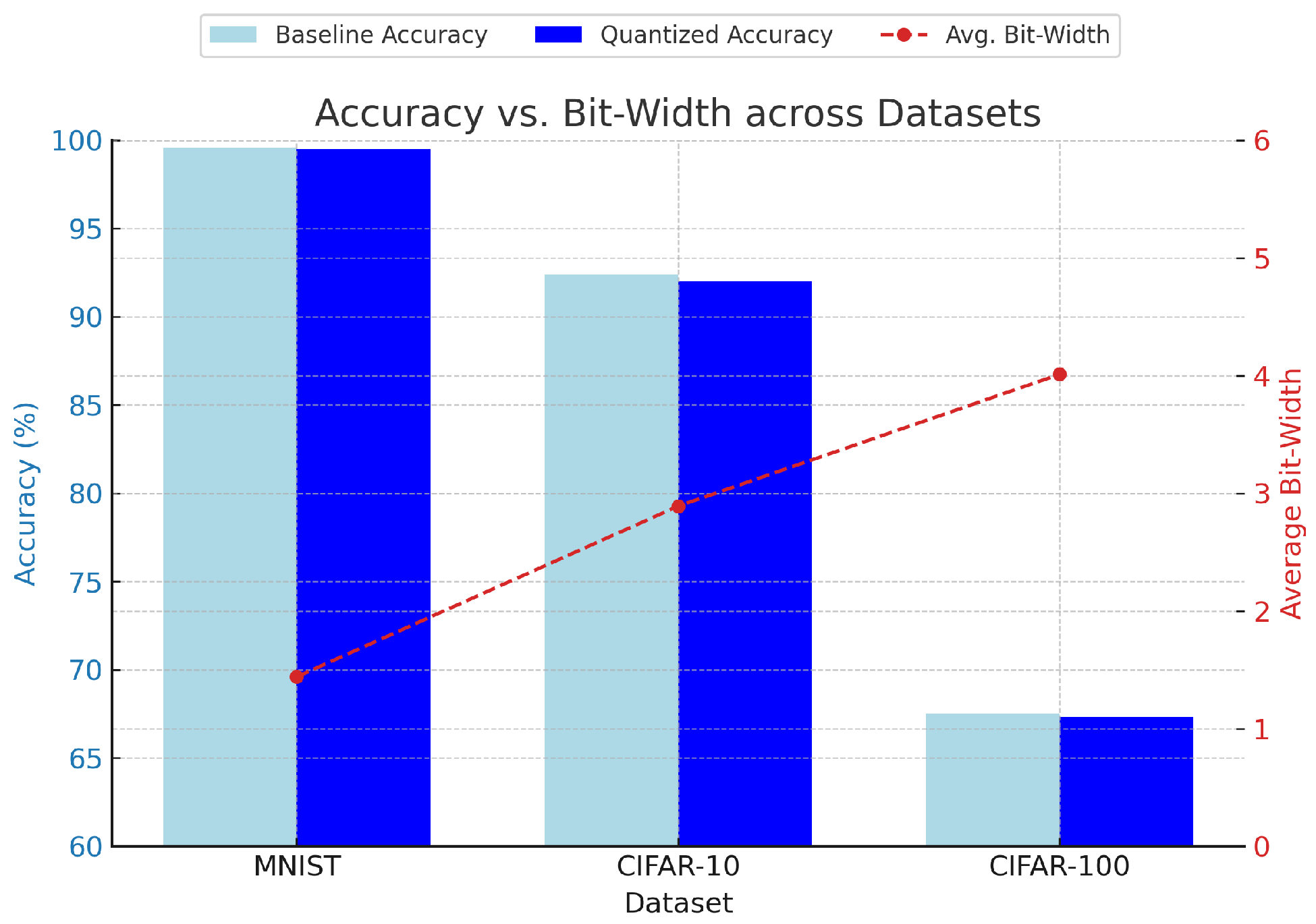
Figure 4 illustrates the trade-off between accuracy and the average bit-width across three standard benchmarks: MNIST, CIFAR-10, and CIFAR-100. Our method consistently reduces bit-widths while maintaining accuracy within 1% of the full-precision baseline.

5.3. MNIST Evaluation

For MNIST, a simple handwritten digits dataset, we used $\lambda =0.5$.

Table 2. Performance comparison on MNIST.

Model Type	Accuracy (%)	Bit Penalty	Avg. Bit-Width
Baseline model	99.58	1.634	16.0
Quantized Model	99.52	0.256	1.44

shows a negligible accuracy drop ($<0.1\%$) with the average per-layer bit-width reduced from 16 to 1.44 bits.

Our method discovered that nearly all layers could be reduced to binary precision—using only the sign bit—while preserving near-perfect accuracy. This confirms prior findings in [13,15] and further validates the effectiveness of our adaptive approach.

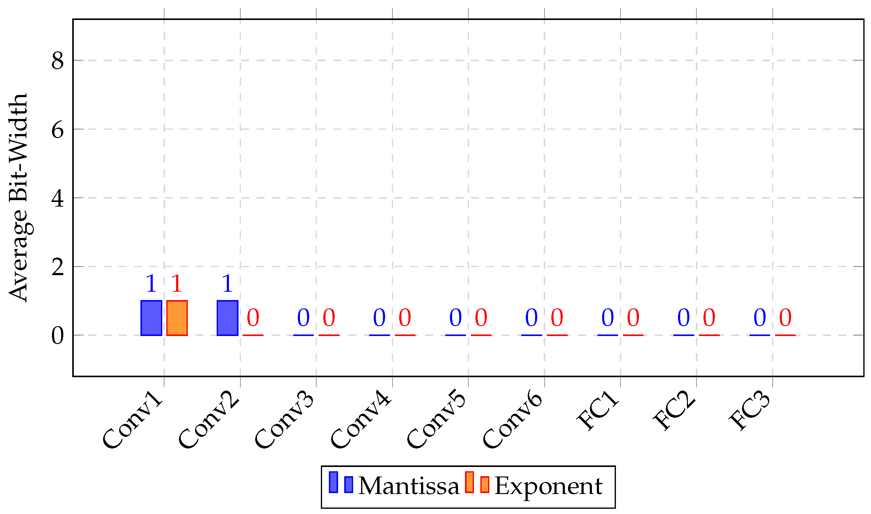
The MNIST model converged to almost entirely fixed-point representations ($b_e=0$) beyond the second convolution. The learned bit-width allocation is given in Figure 5. Only the first two layers use floating-point behavior, and even then, at minimal bit-widths. Fully connected layers use pure fixed-point with mantissa $b_m=0$, effectively binarized. This reflects MNIST’s low numeric complexity.

5.4. CIFAR-10 Evaluation

CIFAR-10 presents a more challenging classification task. With $\lambda =0.5$, our quantized model achieved 91.97% accuracy compared to the 92.36% full-precision baseline (

Table 3. Performance comparison on CIFAR-10.

Model Type	Accuracy (%)	Bit Penalty	Avg. Bit-Width
Baseline	92.36	2.099	16.0
Quantized Model	91.97	0.654	2.89

), while reducing average bit-widths to just 2.89.

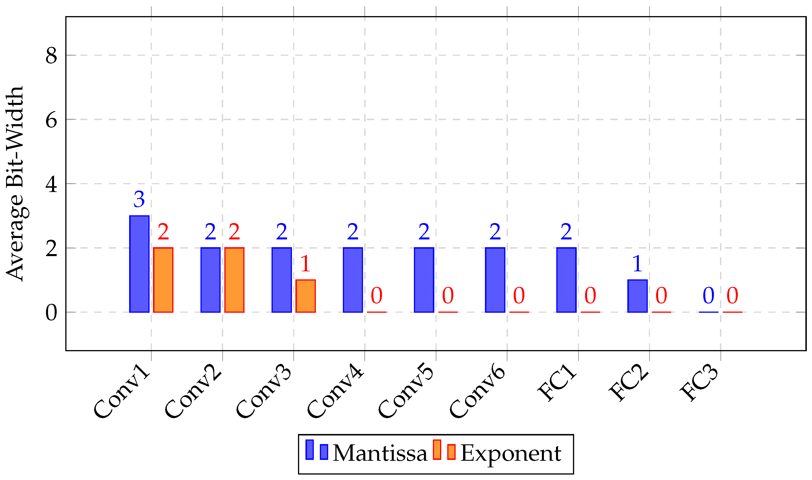
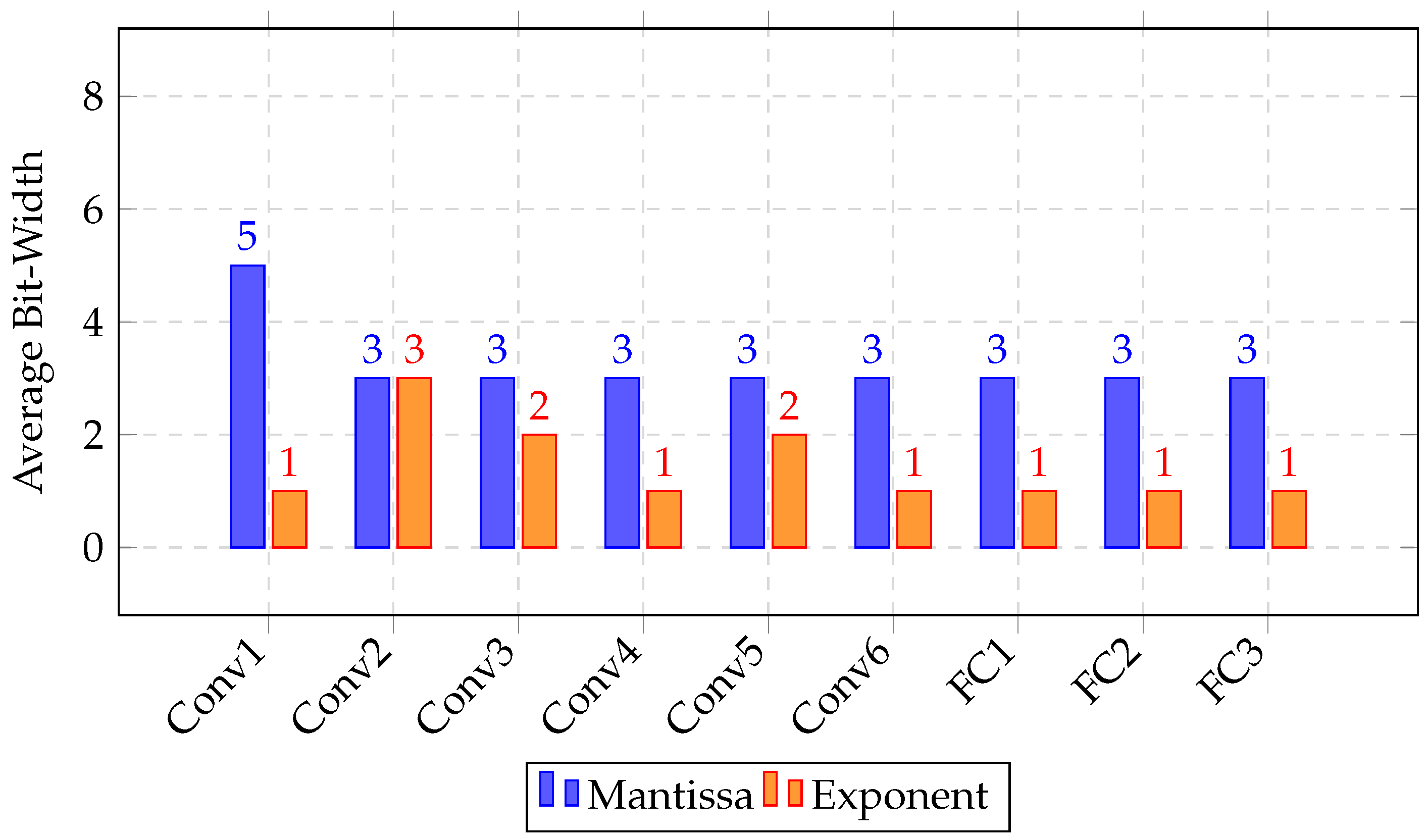
Notably, early convolutional layers retained more exponent bits ($b_e>0$), implying higher sensitivity to quantization noise. Conversely, later layers—including all linear stages—approached near-binarization, as illustrated in Figure 6. This supports previous findings that initial layers are more critical to network representation [4].

For CIFAR-10, early convolutional layers maintain a floating-point style (e.g., conv1 has $b_e=2$, $b_m=3$), reflecting higher numeric range requirements. From conv4 onward, the exponent collapses to zero, and the network favors fixed-point. Linear layers aggressively minimize precision. This shows precision-aware adaptation, especially between early and late layers.

5.5. CIFAR-100 Evaluation

CIFAR-100, containing 100 classes, poses significant classification difficulty. With $\lambda =0.01$, we obtained only a 0.17% accuracy drop while compressing precision from 16.0 to 4.01 bits on average (

Table 4. Performance comparison on CIFAR-100.

Model Type	Accuracy (%)	Bit Penalty	Avg. Bit-Width
Baseline model	67.50	4.212	16.0
Quantized Model	67.33	3.247	4.01

).

This demonstrates that our method automatically adjusts the precision to the dataset complexity, allocating more bits when necessary and reducing when possible.

CIFAR-100’s increased task complexity results in consistently higher bit-widths across all layers. As illustrated in Figure 7, conv1 uses a full six bits ($b_e+b_m=6$), and even linear layers retain moderate floating-point usage. The network converges to a hybrid representation, allocating precision to both dynamic range ($b_e$) and resolution ($b_m$) depending on the layer.

5.6. Per-Layer Quantization Behavior

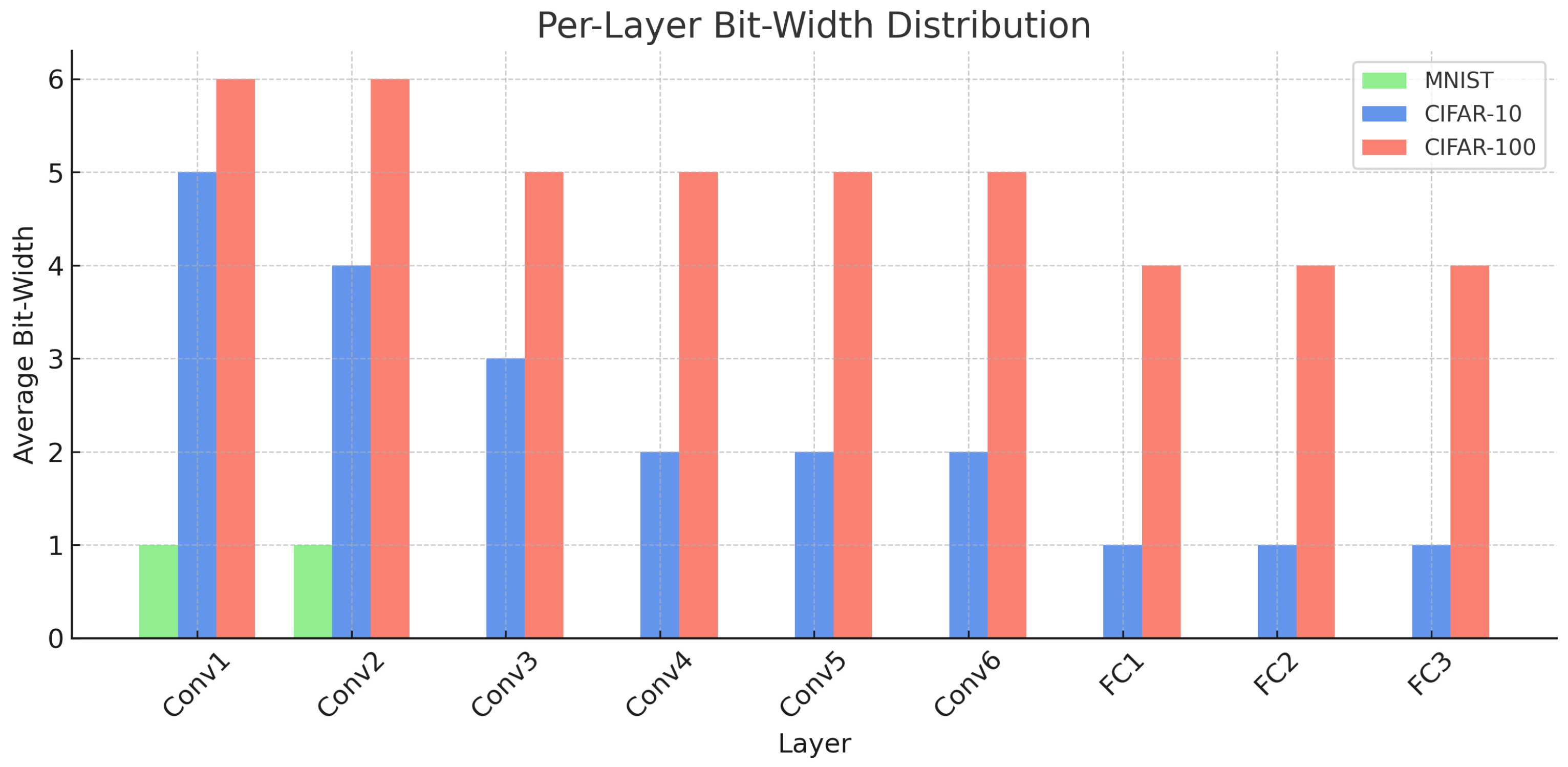
Figure 8 visualizes the learned bit-width distributions across layers. MNIST layers are nearly all binarized, while CIFAR-10 and CIFAR-100 reserve more bits for early convolutions.

5.7. Comparison with Previous Methods

We benchmark our method against several leading quantization-aware training (QAT) approaches on the ResNet-20 architecture with the CIFAR-10 dataset.

Table 5. Comparison of state-of-the-art mixed–precision quantization methods on ResNet-20/CIFAR-10. “Avg. Bit-Width” denotes average precision used for weights (W) and activations (A).

Method	Avg. Bit-Width (W/A)	Top-1 Accuracy (%)	Notable Features
LQ-Nets [19]	2.0/2.0	90.2	Static policy, learned quantization levels
HAWQ-V1 [18]	3.89/4.0	92.2	Hessian-based mixed-precision search
SDQ [27]	1.93/32.0	92.1	Differentiable search, FP activations retained
AdaQAT [10]	3.0/4.0	92.2	Meta-learned quantization-aware training
Ours	3.9/3.9	91.3	Unified format, end-to-end trainable, FPGA-ready

summarizes the accuracy and average bit-width usage for weights and activations. These baselines include LQ-Nets [19], which employ a layer-wise heuristic search; HAWQ-V1 [18], based on Hessian sensitivity analysis; SDQ [27], a differentiable quantization search framework keeping activations at full precision; and AdaQAT [10], which uses meta-learned quantization scheduling.

While these techniques achieve strong performance, they rely on fixed numeric formats and often require external scheduling or auxiliary optimization procedures. In contrast, our approach introduces a fully differentiable framework that jointly learns both the numeric representation and the bit-widths for each layer in an end-to-end fashion. The precision parameters are directly optimized through backpropagation using exponential reparameterization and numerical gradient estimation, enabling the model to smoothly allocate computational precision where needed. Furthermore, unlike prior work that assumes either fixed-point or quantized floating-point formats, our method flexibly spans both through a unified parameterization that adapts per-layer representations during training.

Our model achieves a top-1 accuracy of 91.3% using an average of 3.9 bits for both weights and activations, which is highly competitive with AdaQAT (92.2% at 3/4 bits) and HAWQ-V1 (92.2% at 3.89/4). Notably, this performance is obtained without discrete policy sampling or reinforcement-based exploration. Training is also efficient: the baseline model converges in 53 min, and the quantized fine-tuning phase takes 135 additional minutes, yielding a total cost that remains within the $2.5\times$ range that is typical of QAT pipelines.

Importantly, our bit configurations are directly usable in hardware synthesis flows such as FINN, with FPGA deployment confirming substantial resource savings. This highlights an essential strength of our framework: it produces not only accurate models, but ones that are inherently hardware-aligned and numerically efficient, requiring no hand-tuned quantization heuristics.

5.8. Floating-Point Quantization in Precision-Critical Networks: U-Net Case Study

The results on MNIST, CIFAR-10, and CIFAR-100 indicate that many classification tasks can tolerate aggressive reductions in precision, often converging to near-binarized representations with negligible accuracy loss. While this confirms that fixed-point quantization is sufficient in lightweight recognition problems, it does not address networks whose representational demands extend beyond low-bit fixed-point formats. Dense prediction models such as U-Net, which combine deep encoding paths with high-resolution decoding, are characterized by large dynamic ranges, skip connections, and fine-grained spatial outputs. These characteristics make them substantially more sensitive to quantization noise and therefore an excellent benchmark for assessing the necessity of floating-point quantization.

We investigate this hypothesis by training two quantization-aware variants of U-Net on the DIODE dataset for monocular depth estimation. Both networks adopt identical encoder–decoder architectures and training protocols, differing only in their quantization scheme:

• QUNetFixed: a fixed-point variant in which each layer learns a single bit-width parameter $n_{\ell }$ shared by weights and activations.
• QUNetFloat: a floating-point variant in which each layer learns independent exponent and mantissa bit-widths $(e_{\ell },m_{\ell })$, allowing both numeric range and resolution to be adapted.

• Optimization is performed using Adam with an $L_1$ loss on depth, and quantization parameters are updated jointly with network weights through the straight-through estimator.

Table 6. Comparison of adaptive fixed-point and floating-point quantization on U-Net (DIODE dataset).

Model	Validation MAE	Mean Bit-Width
Baseline (FP32)	2.81	32.0
QUNetFixed	2.84	8.41
QUNetFloat	2.84	6.01

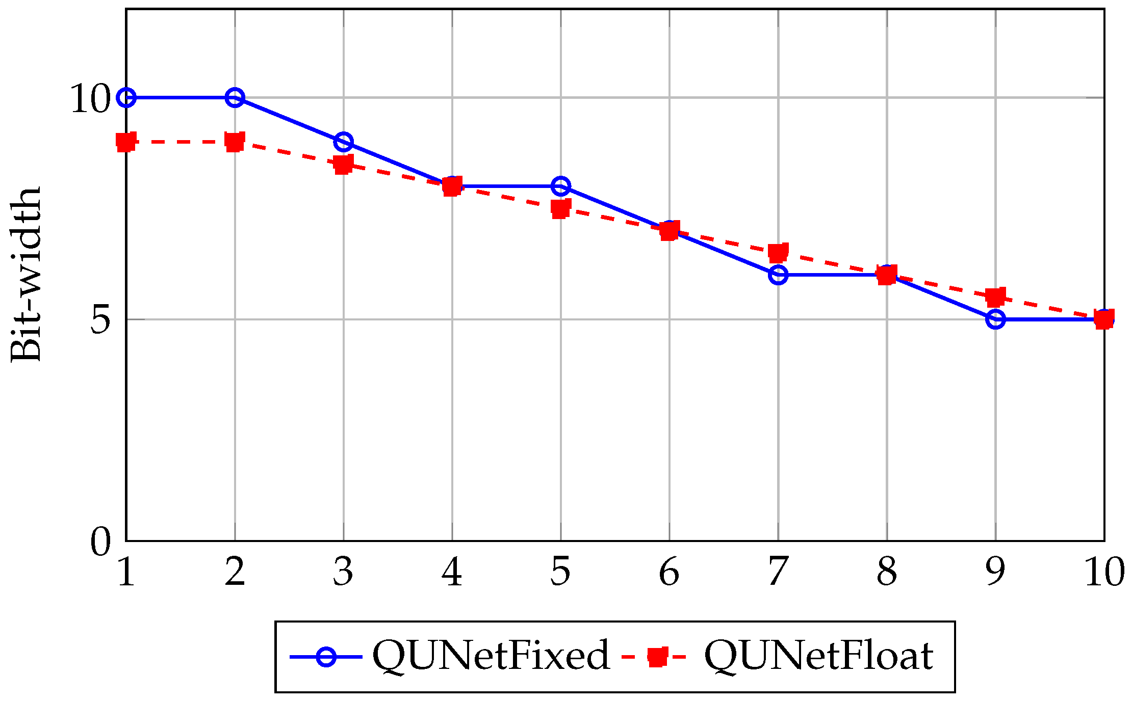
summarizes the results. Both models achieve a nearly identical validation error (∼2.84 MAE), yet QUNetFloat converges to a substantially lower mean bit-width (6.01 vs. 8.41). This corresponds to a ∼29% reduction in precision and, consequently, a proportional reduction in memory footprint and energy consumption during inference. The fact that floating-point achieves equal accuracy at a lower precision highlights that exponent bits provide a greater expressive capacity than mantissa-only increments in fixed-point systems. In other words, floating-point precision enables the network to allocate representational capacity where dynamic range is critical, rather than inflating mantissas across all layers.

The distribution of learned precision across U-Net layers, shown in Figure 9, reveals a clear difference in allocation strategies. In QUNetFixed, early encoder layers retain wide mantissas to preserve accuracy, since the format lacks exponents to cover high dynamic ranges efficiently. By contrast, QUNetFloat introduces exponent bits in these same layers, which allows the mantissa width to shrink significantly without compromising range. This hybrid allocation not only reduces the total bit-width but also reflects the intrinsic numeric demands of encoder–decoder architectures: a wide range is critical in feature extraction, whereas high resolution is primarily needed in late decoding stages. Our framework captures this distinction automatically through gradient-based optimization of precision parameters.

These findings demonstrate that while fixed-point quantization is sufficient for small-scale classification networks, it becomes less efficient for precision-critical architectures such as U-Net. Floating-point quantization achieves the same predictive performance at lower precision by leveraging exponents to capture wide dynamic ranges. This property directly translates into reduced memory traffic and energy consumption in hardware accelerators, as fewer bits need to be stored and transferred per layer. Consequently, floating-point quantization is advantageous in scenarios where a dynamic range is an intrinsic property of the task.

5.9. FPGA Implementation and Hardware Validation

To validate the practical deployability of our learned quantized model, we implemented the CIFAR-10 network on the Pynq-Z2 FPGA platform using the FINN framework [5]. FINN supports fully quantized inference pipelines and is widely used for prototyping ultra-low-precision neural networks. However, as FINN currently lacks support for floating-point operators, the few layers in our network that were learned as floating-point (i.e., with nonzero $b_e$ values) were approximated using equivalent fixed-point bit-widths matching their total effective resolution.

The synthesis results are shown in

Table 7. FPGA synthesis results for CIFAR-10 model on Pynq-Z2 using FINN.

Resource	Baseline (16-Bit)	Optimized (Learned Bitwidths)
LUTs	4800000	34800
Flip-Flops (FFs)	221000	58400
DSPs	31	31
BRAMs	6915	1220
FMAX (MHz)	103.82	102.34
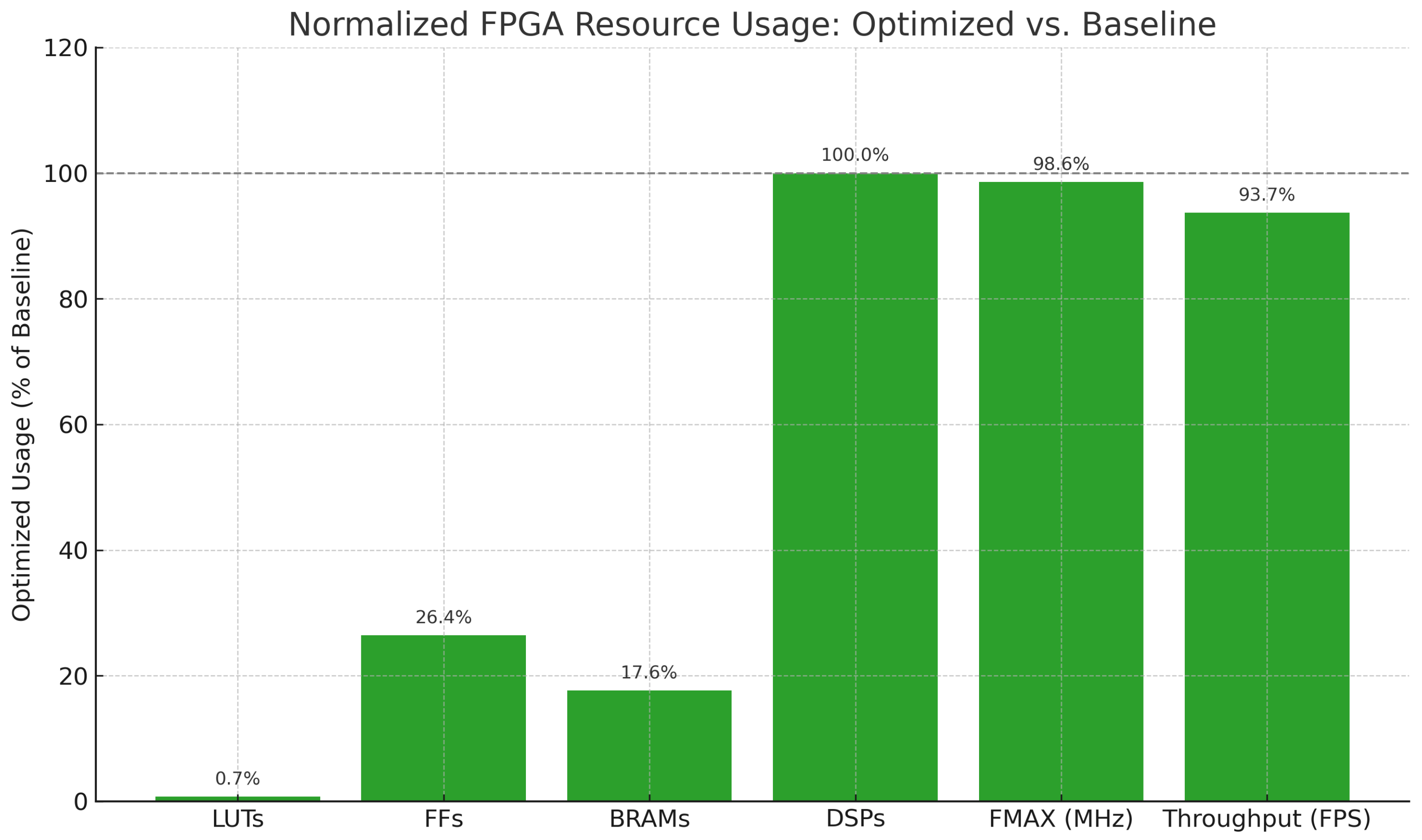
Throughput (FPS)	11.1	10.4

. Compared to the full-precision 16-bit baseline model, the bit-optimized network achieves a dramatic reduction in hardware resource utilization: over $130\times$ fewer look-up tables (LUTs), $3.8\times$ fewer flip-flops (FFs), and $5.6\times$ fewer block RAMs (BRAMs), while maintaining identical DSP usage. Notably, the drop in operating frequency (FMAX) and throughput is negligible, confirming that quantization leads to compact implementations without bottlenecking performance.

These results demonstrate the strength of our proposed bit-aware training in delivering hardware-efficient neural networks. The reduced bit-widths—learned via gradient descent—translate into fewer logic elements and memory blocks at deployment. Importantly, the hardware gains are not linearly proportional to average bit-width, but often exceed expectations due to more efficient resource mapping by the synthesis toolchain. As predicted by the bit-aware loss (Section 4.4), lower bit-widths reduce LUT/BRAM usage nonlinearly due to FPGA resource mapping optimizations.

In addition to resource usage, these reductions also imply significant energy savings. On FPGAs, dynamic power consumption scales approximate linearly with active logic (LUTs/FFs) and on-chip memory (BRAMs). Given the measured $5.6\times$ reduction in BRAMs and >5× reduction in LUTs, we conservatively estimate that the optimized model requires only ∼45–$60\%$ of the total power of the 16-bit baseline, as observed in Figure 10, depending on the static-to-dynamic power ratio of the device. Since throughput remains nearly identical, this translates directly into a ∼40–$55\%$ reduction in energy per inference. These estimates strengthen the argument that our method not only reduces resource utilization but also enhances energy efficiency, a key requirement for edge-AI deployment.

Moreover, this demonstrates that mixed-precision quantization—when co-designed with hardware constraints—can achieve favorable deployment trade-offs even in constrained environments. Our framework not only reduces the arithmetic cost but also the memory footprint and I/O bandwidth, all of which are critical for embedded and edge-AI deployments. The model’s ability to selectively use lower precision in linear layers and higher precision in early convolutional layers aligns well with hardware cost asymmetry, confirming the effectiveness of our end-to-end bit-aware optimization.

Beyond FINN, our quantization framework is portable to other FPGA toolchains such as HLS4ML and Vitis AI. Since it produces layer-wise bit-widths and numeric formats as integer parameters, the learned configurations are backend-agnostic. Fixed-point mappings are directly supported in both HLS4ML and Vitis AI, while hybrid floating-point layers require extending datatype libraries or defining custom operators. Although native floating-point support in these toolchains remains limited, our framework provides deployment-ready bit-width schedules that are adaptable across ecosystems, with the main constraint being the availability of compact floating-point primitives.

6. Discussion

The results of our study demonstrate the effectiveness and originality of the proposed bit-aware quantization framework, which jointly learns numerical precision and task-specific parameters through end-to-end training. Across MNIST, CIFAR-10, and CIFAR-100, our method consistently reduced average bit-widths by up to $5\times$ compared to baseline full-precision or fixed-precision models—while maintaining accuracy within <1% of the original models.

One of the most significant contributions lies in the introduction of a fully differentiable bit-aware loss function, which enables the dynamic and continuous adaptation of bit-widths. Unlike heuristic or layer-wise greedy approaches, our method treats exponent and mantissa bit-widths as learnable parameters, optimized through gradient descent. This flexibility allows each layer to autonomously converge toward a locally optimal numeric configuration, conditioned by both the data and the task complexity.

In comparison to prior mixed-precision quantization methods such as HAWQ [18], AdaQAT [10], and SDQ [27], our approach introduces a unified representation for fixed- and floating-point formats, significantly broadening the expressiveness of the learned quantization. This not only enables seamless adaptation between integer and floating-point behaviors but also yields bit-width configurations that better align with the needs of each layer, as evidenced by the learned per-layer bit allocations in Section 5.

It is important to note that FPGAs typically avoid floating-point arithmetic not merely due to bit-width considerations, but because floating-point operators require substantially more DSPs, LUTs, and flip-flops than fixed-point. Our current hardware validation, performed using the FINN framework, therefore mapped learned floating-point layers to equivalent fixed-point widths. This approximation underestimates the true operator overhead of floating-point arithmetic. However, our framework minimizes the number of layers that rely on floating-point, limiting the potential resource impact while still capturing its benefits in terms of dynamic range. Moreover, the U-Net case study in Section 5 highlights that floating-point can actually reduce the mean bit-width (6.0 vs. 8.4 for fixed-point) at equal accuracy, leading to lower memory traffic and system-level efficiency gains despite higher per-operation cost.

Furthermore, we validated our approach through hardware synthesis on an FPGA target (Pynq-Z2), demonstrating a practical reduction in resource usage: >5× LUT savings and >4× BRAM savings, with negligible throughput loss. This hardware validation highlights the deployability of our approach in real-world, resource-constrained environments such as edge devices and embedded AI systems.

From a training perspective, our approach incurs only moderate computational overhead. While mixed-precision training adds a bit-penalty gradient path, it avoids the architectural duplications or search-tree expansions required by differentiable NAS or RL-based quantization methods. The reported training time overhead of ∼2.5× remains competitive, particularly given the granularity of the optimization and its hardware-aligned outcomes.

Overall, our findings suggest that bit-width can be treated not merely as a post-hoc compression choice, but as a first-class learnable variable that integrates naturally into modern deep learning optimization. The demonstrated balance between performance, compression, and deployability confirms the potential of our method to serve as a general framework for precision-adaptive training. A more complete comparison of fixed-point and floating-point operator costs on FPGA hardware will be pursued as future work.

6.1. Implications for Runtime Reconfigurability

An additional avenue opened by our framework lies in its potential synergy with runtime reconfigurable FPGA deployments. Because bit-widths and numerical formats are learned at a fine-grained, per-layer level, the resulting models naturally lend themselves to adaptive execution strategies. For instance, bitstream switching or partial reconfiguration could enable different precision profiles to be deployed under varying workload or energy constraints—using lower-precision mappings during latency-critical operation and higher-precision profiles when accuracy is paramount. Similarly, layer-wise tuning of numerical formats at runtime could reduce the need for over-provisioning, allowing embedded devices to balance performance and efficiency in situ. While our present work demonstrates static deployment configurations, the ability to treat numerical precision as a learnable variable provides a foundation for future systems in which precision settings are not only optimized during training but also adapted dynamically at inference time.

6.2. Cost of Hybrid Floating-Point Implementations

Although learnable floating-point layers improve accuracy and dynamic range, they introduce higher hardware costs on FPGAs due to additional logic for normalization and exponent handling. In our study, these layers were emulated with fixed-point precision in FINN, which underestimates the true operator overhead. However, this impact remains limited since only a few layers adopt floating-point and reduced mantissa widths and lower BRAM usage.

From an operator perspective, supporting a true hybrid format requires additional FPGA resources, particularly for floating-point adders and multipliers. Floating-point multipliers typically consume both DSP slices and LUTs for exponent alignment, while adders require normalization logic beyond fixed-point equivalents. Nevertheless, because our framework restricts floating-point usage to only a few precision-critical layers, the incremental DSP and LUT overhead remains limited compared to a fully floating-point implementation. In practice, the observed memory savings and reduced BRAM traffic offset these costs at the system level, highlighting the trade-off between per-operator complexity and overall efficiency.

6.3. Fixed Data Width vs. Learned Formats

Our framework primarily explores the joint optimization of bit-width and format, but the two can also be decoupled. If the overall width is fixed (e.g., 16 bits), the learnable format still provides benefits by redistributing bits between exponent and mantissa, effectively adapting the numeric range per layer. While we did not explicitly benchmark this fixed-width scenario, prior studies suggest that mixed representations can preserve accuracy at narrower mantissas, especially in early convolutional layers. The additional FPGA cost of supporting a hybrid structure arises mainly from floating-point normalization logic, as discussed in the previous subsection, and remains bounded since only a few layers typically converge to floating-point behavior.

6.4. Limitations and Future Directions

This work, while demonstrating the effectiveness of learnable hybrid quantization, also carries certain limitations that suggest directions for future research. First, the current implementation is tightly coupled to PyTorch with custom autograd operators; although this choice enables rapid prototyping, it may restrict direct portability to alternative training frameworks. Second, the gradient-based relaxation used for bit-width learning can exhibit numerical sensitivity in extreme low-precision regimes, warranting further study of more stable estimators. Finally, our hardware validation employed the FINN toolchain, which approximates floating-point layers with equivalent fixed-point implementations; as such, the precise overhead of native floating-point operators on FPGAs remains to be quantified. These constraints do not detract from the central contributions of the work—namely, demonstrating that precision itself can be treated as a learnable parameter—but rather outline clear avenues for extending the framework toward broader applicability and more comprehensive hardware characterization.

7. Conclusions

This work introduced a novel, unified framework for quantization-aware training that learns both the numerical format and the bit-width configuration in an end-to-end differentiable manner. By leveraging a flexible numeric representation that is capable of emulating both fixed-point and floating-point arithmetic, our method enables fine-grained, layer-wise precision adaptation—eliminating the need for manual bit allocation or an expensive neural architecture search.

We further proposed a bit-aware loss function that regularizes model complexity by penalizing excessive bit usage during training. This leads to compact, hardware-efficient neural networks that retain high task performance while significantly reducing resource demands. Extensive evaluations across datasets such as MNIST, CIFAR-10, and CIFAR-100 demonstrate the method’s ability to maintain competitive accuracy at drastically reduced average bit-widths.

Beyond algorithmic performance, we validated the real-world applicability of our approach through FPGA synthesis using the Xilinx FINN framework. The resulting models exhibited over $5\times$ reductions in logic and memory resources compared to standard 16-bit quantization baselines, while maintaining comparable throughput and latency. As FINN does not natively support floating-point, hybrid layers were approximated using fixed-point equivalents, which underestimates the operator overhead of floating-point arithmetic. Nevertheless, our framework minimizes floating-point usage to only a small number of precision-critical layers, and our U-Net case study shows that floating-point can achieve equal accuracy at a lower mean precision than fixed-point, thereby reducing memory traffic and improving system-level efficiency.

In summary, our approach provides a principled path toward precision-adaptive deep learning—uniting task-aware learning objectives with hardware-aligned constraints. Future directions include extending this framework to transformer-based architectures, integrating it into end-to-end compiler flows, and performing a complete comparison of fixed-point and floating-point operator costs on FPGA hardware. We also aim to investigate precision-adaptive training under dynamic workload or latency constraints.