Abstract
To address the limitations of the traditional methods that are used to extract features from non-stationary signals and capture temporal dependency relationships, a rolling bearing fault diagnosis method combining variational mode decomposition (VMD) and deep learning is proposed. A hybrid VMD-CNN-Transformer model is constructed, where VMD is used to adaptively decompose bearing vibration signals into multiple intrinsic mode functions (IMFs). The convolutional neural network (CNN) captures the local features of each modal time series, while the multi-head self-attention mechanism of the Transformer captures the global dependencies of each mode, enabling the global analysis and fusion of features from each mode. Finally, a fully connected layer is used to classify the 10 fault types. The experimental results on the Case Western Reserve University bearing dataset demonstrate that the model achieves a fault diagnosis accuracy of 99.48%, which is significantly higher than that of single or traditional combined methods, providing a new technical path for the intelligent diagnosis of rolling bearing faults.
1. Introduction
In the modern industrial landscape, rotating machinery is a critical piece of equipment across various production sectors. As a core component of such machinery and a fundamental and vital part of modern industry, rolling bearings are prone to developing failures of varying severity during operation due to long-term, high-intensity rotational friction, which can result in significant losses [1,2,3]. According to relevant studies, bearing failures account for approximately 30% to 40% of mechanical failures in modern industrial systems [4].
With the advancement of industrial intelligence, the fault diagnosis of bearings under complex working conditions has become increasingly critical [5]. Traditional fault diagnosis methods largely rely on manually designed features and are implemented in conjunction with classical signal processing techniques such as empirical wavelet transform (EWT) and empirical mode decomposition (EMD). Nevertheless, such methods exhibit distinct shortcomings when adapting to the demands of rolling bearing fault diagnosis.
Specifically, EWT [6] necessitates the prior a priori segmentation of the Fourier spectrum of the signal. However, the segmentation rules (e.g., threshold setting) frequently depend on manual tuning, which renders it challenging to adapt to the variations in vibration signals induced by different types of rolling bearing faults (such as inner race, outer race, and rolling element faults). Concurrently, EWT requires the adjustment of a larger number of parameters, which further escalates the computational cost. On the other hand, the core issue with empirical mode decomposition resides in its propensity to exhibit the phenomenon of “mode mixing” during the decomposition process. This phenomenon is specifically manifested in two aspects: signal components with different frequencies are inadvertently merged into the same intrinsic mode functions (IMFs), or signal components with the same frequency are inappropriately split into multiple IMFs. Ultimately, this leads to the decomposed modes losing their clear physical significance. Given that the fault signals of rolling bearings themselves inherently possess intricate frequency components (e.g., the superposition of fault impact frequencies and normal operating vibration frequencies), such mode mixing directly impedes the accurate separation of fault features.
Furthermore, the vibration signals of rolling bearings also demonstrate prominent features, including non-stationarity, multi-scale characteristics, and intense noise interference. These inherent properties result in the aforementioned traditional methods encountering substantial limitations in both fault feature extraction and temporal dependency modeling. Consequently, they are incapable of meeting the need for high accuracy and robust reliability in rolling bearing fault identification under complex industrial scenarios [7].
In recent years, with the development of machine learning and deep learning technologies, these methods have also been introduced into the field of fault diagnosis, bringing new research directions and solutions [8,9,10]. Existing deep learning-based methods have made progress in specific scenarios, but critical challenges remain unresolved, especially in addressing the non-stationarity of vibration signals and the complexity of multi-scale feature fusion:
- Limitations in long-range temporal dependency modeling: Methods such as the IWOA-VMD-KELM model [11] use the improved whale optimization algorithm (IWOA) to optimize variational mode decomposition (VMD) parameters and rely on kernel extreme learning machine (KELM) for classification. While VMD enhances feature extraction, KELM—a traditional machine learning classifier—lacks the ability to capture long-range temporal dependencies in sequential vibration data, which becomes a critical shortcoming when dealing with dynamic fault evolution processes (e.g., the gradual expansion of bearing cracks).
- Insufficiency in global feature correlation: The WI-CNN model [12], which integrates adaptive stochastic resonance denoising and the Gramian angular field-based convolutional neural network (CNN), strengthens weak fault features through preprocessing and spatial transformation. However, it relies solely on the CNN for local spatial feature extraction and fails to model the global correlations between decomposed modal components. This oversight often leads to incomplete feature representation when faults exhibit multi-scale propagation characteristics.
- Suboptimal decomposition of strongly non-stationary signals: For small-sample scenarios, the ALA-FMD-MSCA-RN framework [13] uses the artificial lemming algorithm (ALA) to optimize feature mode decomposition (FMD) parameters. Nevertheless, FMD lacks the rigorous mathematical foundation of VMD for modal separation, resulting in suboptimal decomposition effects when processing strongly non-stationary bearing vibration signals.
- Difficulty in handling high-dimensional features: The SK-LS-SVM method [14], which combines spectral kurtosis (SK) and the least-squares support vector machine (LS-SVM), can effectively identify fault-related frequency bands. However, the LS-SVM struggles to handle high-dimensional features extracted from complex vibration signals, leading to a reduction in the accuracy of multi-fault classification tasks (e.g., simultaneously distinguishing inner ring, outer ring, and rolling element faults).
To address the aforementioned challenges, this paper proposes a hybrid VMD-CNN-Transformer model for rolling bearing fault diagnosis. The core design logic of this model lies in leveraging the complementary advantages of three key components: first, VMD is used to adaptively decompose non-stationary vibration signals into multiple intrinsic mode functions with clear physical meanings, thereby enhancing signal stability and fault feature separability; second, the CNN is employed to extract local temporal features (e.g., transient fault impulses) from each IMF component, leveraging its strengths in local perception and weight sharing; and finally, the Transformer’s multi-head self-attention mechanism captures global dependencies across different modal components and time scales, enabling the deep fusion of multi-scale features. This synergistic design not only solves the problem of insufficient feature extraction from non-stationary signals, but also overcomes the limitations of single models in capturing temporal dependencies, providing a more efficient and reliable technical path for intelligent rolling bearing fault diagnosis.
2. Materials and Methods
2.1. Data Acquisition and Preprocessing
2.1.1. Data Source
This study employs the Case Western Reserve University (CWRU) open access rolling bearing dataset as the experimental benchmark [15,16]. The test bench for obtaining the CWRU bearing dataset is shown in Figure 1. This test bench is mainly composed of an electric motor, a drive-end bearing, a torque transducer and encoder, and a dynamometer [17]. Among these, the electric motor, as a power source, provides driving force for the operation of the system, simulating the power input environment of the bearing in actual work; the drive-end bearing is the core test object, can simulate fault forms such as wear, crack, and pitting through artificial setting or natural deterioration, and is used to collect fault characteristic data; the torque transducer and encoder is used to measure the torque transmitted between the motor output shaft and the load, assist in monitoring the mechanical characteristics of the system, and analyzes the stress state of the bearing during operation; and the dynamometer applies resistance to the test bench, simulating the external load of the bearing in actual working conditions, making the test environment similar to an industrial scene, so as to obtain more practically valuable data. Single-point faults are manufactured on the bearing by electric discharge machining, and the fault diameters include specifications such as 7 mils, 14 mils, and 21 mils, covering the inner raceway, rolling elements, and outer raceway [18]. Vibration data are collected by accelerometers installed at the drive end and fan end (fan-end bearing position) of the motor housing, with two sampling frequencies of 12 kHz and 48 kHz. The collected data are processed in MATLAB2018b or later versions. This study uses the condition data of the drive-end bearing under a sampling frequency of 12 kHz, a motor load of 0 HP, and a rotational speed of 1797 r/min.
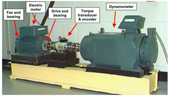
Figure 1.
Bearing test bench.
2.1.2. Data Preprocessing
Rolling bearing faults mainly include inner ring faults, outer ring faults, and rolling element faults, as illustrated in Figure 2. In this study, the collected bearing data were analyzed; this included normal (fault-free) data and the fault data of inner rings, outer rings, and rolling elements with fault diameters of 7 mils, 14 mils, and 21 mils, respectively. This forms a dataset containing 10 distinct categories [19], and the specific category details are presented in Table 1 below. The samples from the 10 different categories in the dataset underwent normalization processing. By mapping each feature value to the interval [0, 1], the interference of different dimensions in model training was effectively eliminated. This enables the model to learn data features more accurately, thereby improving the performance metrics of fault diagnosis, including precision and accuracy. Subsequently, variational mode decomposition was applied to the normalized data, decomposing complex non-stationary signals into several stable intrinsic mode functions. This process provides input signals with physical significance for the subsequent extraction of features. Then, a sliding window technique was adopted to segment the dataset into samples by configuring the window size, step size, and overlap ratio. The samples were divided into a training set, a validation set, and a test set in a ratio of 7:1:2. Among these, the training set accounts for 70% of the total number of samples and is mainly used for training model parameters; the validation set accounts for 10% of the total number of samples and is primarily used for optimizing hyperparameters and monitoring overfitting; and the test set accounts for 20% of the total number of samples and is mainly utilized for the final evaluation of generalization.
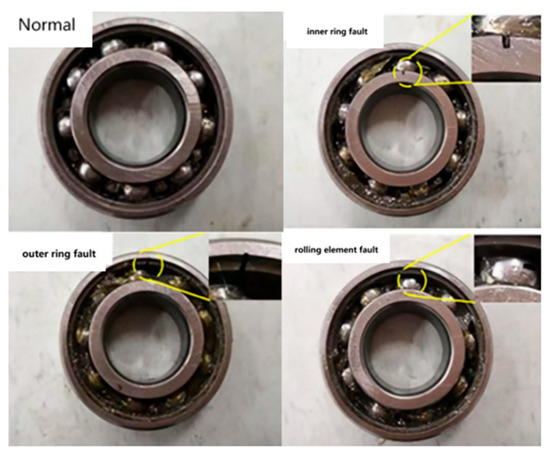
Figure 2.
Diagram of faults in various parts of the bearing.

Table 1.
Classification table of bearing fault categories.
2.2. Basic Method
2.2.1. Variational Mode Decomposition
In the field of rolling bearing fault diagnosis, variational mode decomposition serves as a crucial adaptive signal processing technique [20] that is capable of precisely analyzing the complex non-stationary vibration signals generated during bearing operation. By decomposing the original vibration signal into multiple stationary intrinsic mode functions [21], VMD can effectively extract bearing fault features, facilitating the accurate identification of fault types and severity.
Compared with traditional empirical mode decomposition, VMD introduces a variational framework to optimize the bandwidth of each modal function, demonstrating stronger robustness and anti-noise performance in processing the early weak fault signals of bearings. In practical applications, whether dealing with signals generated by faults such as inner ring spalling, outer ring wear, or rolling element pitting, VMD leverages its advantages of strong adaptability, high robustness, and fast computational efficiency to quickly and accurately extract fault features.
The core mechanism of VMD involves decomposing the bearing vibration signal into multiple intrinsic mode functions with limited bandwidth and non-overlapping frequency bands. This process is achieved by formulating and solving a specific variational optimization problem:
where uk(t) is the k-th modal function, which records the vibration information of different frequency components; represents the central frequency of the -th mode; k denotes the number of modes obtained by decomposition; t is the time variable; is the complex exponential function; f is the original bearing vibration signal; and is the Dirac function.
2.2.2. Convolutional Neural Network
A CNN is a feedforward neural network specifically designed to process grid-like data (such as images and time series signal spectrums). Through the mechanisms of local perception, weight sharing, and downsampling, it has demonstrated excellent performance in fields such as image classification, object detection, and bearing fault diagnosis [22].
The core structure of a CNN includes convolutional layers, activation functions, pooling layers, and fully connected layers [23].
- Convolutional Layer
This layer employs convolution kernels (filters) to traverse the input data and extract local features (such as edges and textures):
where X denotes the input feature map, W represents the convolution kernel weights, b is the bias, and k is the output channel index.
The activation function introduces nonlinear transformations to enhance the model’s expressive capacity. The commonly used ReLU function, (f(x) = max(0, x)), avoids the vanishing gradient problem and accelerates the training process.
- Pooling Layer
Function: The dimensionality of feature maps is reduced and translational invariance is enhanced. The formula for max pooling is as follows:
where denotes the value of the pooled feature map at position (i, j, k), where i and j represent the spatial coordinates, and denotes the number of channels.
represents the value at the corresponding position in the original feature map. s is the pooling stride, and m and n are the coordinates offset within the pooling window R. The pooled value is determined by finding the maximum value within the window R, thus achieving a reduction in dimensionality. By retaining locally prominent features, this operation reduces computational complexity and mitigates the risk of overfitting.
- Fully Connected Layer
This integrates high-level feature maps into classification or regression results, and outputs a probability distribution through the Softmax function.
The architecture of the CNN module constructed in this study is roughly shown in Figure 3 below.
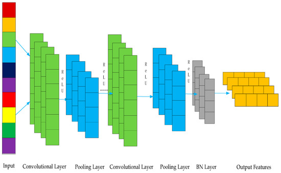
Figure 3.
CNN module architecture.
2.2.3. Multi-Head Self-Attention Mechanism
The multi-head self-attention mechanism [24], a core component of Transformer models, is widely applied in fields such as natural language processing and time series analysis. By computing multiple attention heads in parallel, it extracts information from distinct subspaces, thereby capturing rich features within input sequences. In bearing fault diagnosis, the multi-head self-attention mechanism is employed to further extract global dependencies from the features extracted by the CNN, thereby enhancing the accuracy and robustness of fault diagnosis, as illustrated in Figure 4.
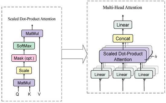
Figure 4.
Multi-head self-attention mechanism.
The multi-head attention mechanism enables the model to capture information from different subspaces by projecting queries, keys, and values into multiple subspaces, computing attention in parallel, and then merging the results. The core formulas are as follows:
- Scaled Dot-Product Attention
In each attention head, the attention score is computed using scaled dot-product attention:
where Q, K, and V denote the query matrix, key matrix, and value matrix, respectively; dk is the scaling factor (typically the dimension of the key vectors); and softmax is the activation function.
- Multi-Head Attention Calculation
After concatenating the outputs of the single-head attention mechanisms, the result is passed through a linear projection matrix to obtain the final output of the multi-head attention mechanism.
where and denote the weight matrices for the query, key, and value matrices of the i-th attention head, respectively. h represents the number of attention heads.
2.2.4. Feature Fusion Module
Inputs to the feature fusion module are the output features of the four intrinsic mode functions (IMFs)—obtained via variational mode decomposition (VMD)—following convolution and pooling operations by a convolutional neural network (CNN). These features are denoted as , each with a dimension of [B, T, D], where B denotes the batch size; T represents the temporal sequence length; and D stands for the feature dimension.
- Cross-Component Attention Weight Calculation
By leveraging the scaled dot-product attention mechanism inherent in multi-head self-attention, the importance weights of each IMF component are computed through the following steps:
① Feature Concatenation: The features of the four IMF components are concatenated along the batch dimension to construct a cross-component feature matrix, which provides a global context for attention computation:
where Fconcat has a dimension of [4B, T, D].
② Query–Key–Value Projection: Through learnable weight matrices, the concatenated features are linearly projected into query (Q), key (K), and value (V) matrices, ensuring consistency with the parameters of the Transformer:
where are the weight matrices.
③ Attention Scoring and Normalization: Attention scores are calculated using the scaled dot-product attention mechanism, and then normalized via the Softmax function to generate attention weights:
The attention output is further split into subsets corresponding to the original four IMF components. For the i-th IMF component, its normalized weight, —which satisfies the constraint ()—is calculated as follows:
where denotes the attention output subset corresponding to the i-th IMF component after splitting, and represents summation over the feature dimension, thereby quantifying the contribution of each IMF component.
- Multi-Component Feature Weighted Fusion
The final fused feature, , is obtained by performing a weighted summation of the features of the four IMF components using the normalized weights, . The dimension of remains [B, T, D]. The fused feature is fed into the fully connected layer, which is used for the classification of 10 types of bearing faults.
2.3. Rolling Bearing Fault Diagnosis Model Based on the VMD-CNN-Transformer Model
This section will detail the rolling bearing fault diagnosis model based on a VMD-CNN-Transformer model. This model innovatively integrates VMD in order to adaptively decompose bearing vibration signals into multiple intrinsic mode functions, CNN’s particular feature extraction capability, and the Transformer’s global dependency modeling. Through multi-stage feature processing and cross-layer interaction mechanisms, it achieves the accurate identification and localization of compound faults in rolling bearings. The rolling bearing fault diagnosis model based on the VMD-CNN-Transformer model is depicted in Figure 5.
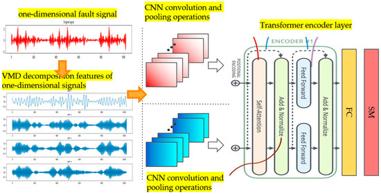
Figure 5.
Rolling bearing fault diagnosis model based on the VMD−CNN−Transformer model.
Here, a CNN captures the local features of each modal time series, and the Transformer models global dependencies. Features from different modal signals are fused and fed into a fully connected layer for fault classification.
The overall processing steps and workflow are as follows:
- (1)
- Data Preprocessing: Denoising and normalization are performed on the acquired data to reduce noise interference and dimensional differences. Subsequently, variational mode decomposition is applied to the data that has undergone denoising and normalization.
- (2)
- Dataset Partitioning: The window size is set to 1024, with an interval step size of 512 and an overlap ratio of 0.5; on this basis, the sliding window technique is employed to segment the original signal into individual samples. Subsequently, the dataset is partitioned into the training set, validation set, and test set at a ratio of 7:1:2, which serves to provide sufficient sample support for the subsequent processes of model training and evaluation.
- (3)
- Construction of the VMD-CNN-Transformer Model: A CNN is used to capture the local features of each modal time series, while a Transformer is employed to capture global dependencies. Finally, the features of different modal signals are fused, and fault classification is completed through a fully connected layer.
- (4)
- Model Training: The parameters of the VMD-CNN-Transformer model are randomly initialized. The Adam optimizer and cross-entropy loss function are selected [25]. Training data is then input in batches. Outputs are obtained through forward propagation, errors are calculated, gradients are computed via backward propagation, and parameters are updated using the optimizer. This cycle continues for a preset number of epochs (50 epochs), with loss and accuracy recorded each epoch to monitor the progress of training [26].
- (5)
- Model Evaluation: Metrics such as accuracy and F1-score are calculated to analyze the model’s classification performance across different fault categories. The cross-entropy loss curve is plotted to observe the model’s convergence behavior, and a confusion matrix is generated to visually illustrate the effectiveness of the model’s classification for each category.
The overall method steps and process are shown in Figure 6 below.
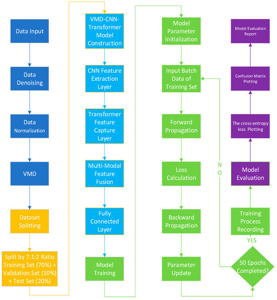
Figure 6.
VMD-CNN-Transformer fault classification method flowchart.
3. Results
3.1. Experimental Results
3.1.1. Experimental Setup
All experiments were conducted on a server equipped with an Intel 13th Gen Core i5-13500HX 14-core processor, 16 GB Micron DDR5 4800 MHz RAM (8 GB + 8 GB), and an NVIDIA GeForce RTX 4050 Laptop GPU (6 GB).
The modal number of VMD is set to 4, and the penalty parameter is set to 2000. The visualization of the VMD results (taking the first 1000 samples of normal vibration signal data as an example) is shown in Figure 7. The rationale for configuring the number of modes in VMD to 4 and the penalty parameter to 2000 is elaborated on as follows:
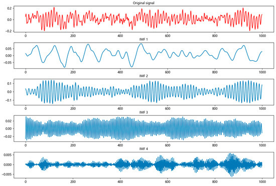
Figure 7.
VMD visualization.
Through a comparative analysis of the central frequency distributions corresponding to K values of 2, 3, 4, 5, 6, 7, and 8, it is determined that setting K = 4 yields optimal results for bearing fault signals. This value enables effective decomposition into low-frequency trend components, fault characteristic frequency components, high-frequency noise components, and medium-frequency modulation components, thereby achieving the precise matching of signal features. Simultaneously, it avoids the under-decomposition that occurs when K < 4 (which fails to fully extract fault characteristics) and the over-decomposition that occurs when K > 4 (which generates spurious modal components), while balancing the efficacy of decomposition with computational efficiency.
A value of α = 2000 was selected based on empirical guidelines for bandwidth constraints, which stipulate that the value should typically range from 1.5 to 2.0 times the length of the sampling points. Given that each data segment processed comprises 1024 sampling points, the reasonable range for α is 1536–2048, with α = 2000 fitting squarely within this interval. This parameter setting effectively restricts the bandwidth of each modal component, prevents mode aliasing, and ensures the separability of the frequency of individual IMF components. Validation through decomposition experiments on four signal states—normal, inner race fault, ball fault, and outer race fault—has confirmed its ability to produce distinct modal separation.
The choices of K = 4 and α = 2000, validated through systematic experimental investigations and theoretical analyses, ultimately guarantee the effectiveness of VMD and the performance of the subsequent CNN-Transformer classification model.
The CNN settings are shown in Table 2. For the Transformer, the number of heads is eight, the dimension of the feedforward network is 256, and the number of layers is two.
Table 2.
Specific parameters of CNN model architecture.
Furthermore, to further explore the impact of the learning rate on the model’s training process, this study sets the learning rates to three gradients: 0.03, 0.003, and 0.0003. By comparing the convergence trends associated with the model’s training loss under different learning rates, the effect on the training performance is analyzed. The relevant experimental results are shown in Figure 8.
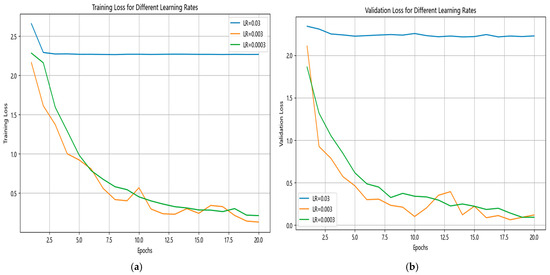
Figure 8.
The impact of different learning rates on model training: (a) training loss for different learning rates; (b) validation loss for different learning rates.
It can be clearly observed from Figure 8 that, when the learning rate is set to 0.0003, the convergence process of the model’s training loss is both relatively fast and has good stability. If the learning rate is increased to 0.003, the model’s training loss shows clear fluctuations, and it will be difficult to achieve convergence stably; when the learning rate is further increased to 0.03, the model’s loss remains very high and hardly decreases. This makes it very difficult for the model to learn effectively and means that it cannot converge.
3.1.2. Model Evaluation Metrics
In the assessment of fault diagnosis models, metrics such as accuracy, precision, recall, and F1-score are commonly utilized as performance indicators. The computational formulas for each metric are as follows:
where TP, TN, FP, and FN denote the counts of true positives, true negatives, false positives, and false negatives, respectively, and i represents the category (i = 0–9).
To further account for the differing importance of fault categories in practical scenarios (e.g., varying severity, occurrence frequency, or business impact), we introduce weighted average versions of the aforementioned metrics. The corresponding formulas are as follows:
where represents the weight, and indicates the weights corresponding to different categories. Here, is directly related to the number of samples in each category.
3.1.3. Algorithm Comparison
To comprehensively evaluate the performance of the VMD-CNN-Transformer model, we compared it against several state-of-the-art fault diagnosis algorithms. The selected benchmark models are as follows:
- IWOA-VMD-KELM: With the improved whale optimization algorithm as the core, it optimizes the number of modal components and penalty coefficient of variational mode decomposition, as well as the regularization coefficient and kernel parameter of the kernel extreme learning machine; VMD decomposes vibration signals to obtain optimal modal components and construct feature vectors, while KELM completes fault classification.
- ALA-FMD-MSCA-RN: For few-shot scenarios, the artificial lemming algorithm is utilized to optimize the parameters of feature mode decomposition, including the number of modes and filter length. Subsequently, the modal components with the minimum Residual Energy Index (REI) are selected and converted into time–frequency maps. The Multi-Scale Coordinate Attention (MSCA) mechanism is employed to enhance key features and combined with a Relation Network (RN) to calculate the similarity of samples, thereby achieving fault classification.
- SK-LS-SVM: Spectral kurtosis adaptively determines the optimal center frequency and bandwidth of vibration signals, and a band-pass filter is constructed to reduce noise. Subsequently, the Hilbert transform is applied to extract the envelope spectrum in order to acquire fault features. Feature vectors are constructed using the signal kurtosis and the amplitude ratio of the characteristic frequencies of the inner and outer rings, which are then input into the LS-SVM to achieve fault classification.
A comparison of the performance of the proposed method and other competing methods on the public bearing dataset from CWRU, with regard to accuracy, is quantitatively presented in Table 3.
Table 3.
Comparison of model accuracies on the CWRU bearing dataset.
Under the benchmark of the CWRU bearing dataset, the VMD-CNN-Transformer exhibits the best performance, with an accuracy of 99.48%. Nevertheless, other methods exhibit unique advantages tailored to specific application scenarios.
Specifically, when aiming to achieve the highest accuracy, the VMD-CNN-Transformer model remains the optimal choice. Under hardware resource constraints, the IWOA-VMD-KELM model offers the best cost-effectiveness, exchanging a mere 0.68% accuracy loss for a substantial reduction in deployment costs. When confronted with the challenge of sample scarcity, the few-shot learning capability of the ALA-FMD-MSCA-RN framework proves irreplaceable. Additionally, when real-time online diagnosis is demanded, the efficiency of the SK-LS-SVM method is unparalleled.
3.1.4. Ablation Experiment
To comprehensively investigate the contributions of individual modules within the VMD-CNN-Transformer model, ablation studies were conducted. The specific experimental results are summarized in Table 4 (including weighted precision, recall, and F1-score) and illustrated in Figure 9. Furthermore, the classification performance of each ablated model was visualized via confusion matrices, as depicted in Figure 10.
Table 4.
Ablation experiment results (performance metrics).
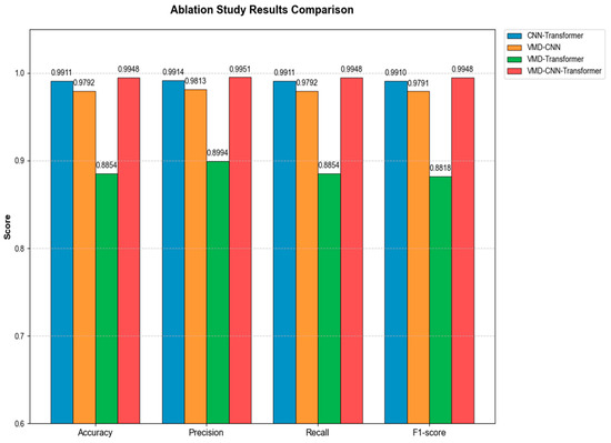
Figure 9.
Comparison chart of ablation experiment results.
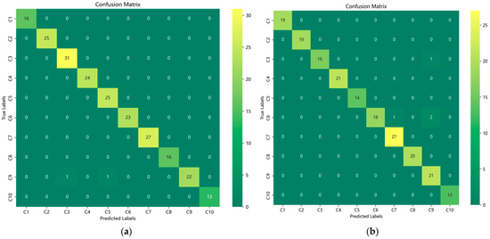
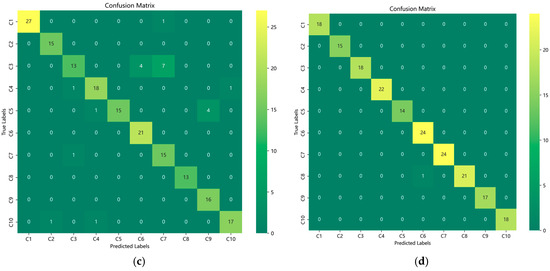
Figure 10.
Confusion matrices of ablation study models: (a) CNN-Transformer confusion matrix; (b) VMD-CNN confusion matrix; (c) VMD-Transformer confusion matrix; and (d) VMD-CNN-Transformer confusion matrix.
In order to conduct a more in-depth evaluation of the practical applicability of the model within industrial contexts, the time required for the model to complete one cycle and its corresponding parameters were systematically documented. The outcomes of this documentation are presented in Table 5 below.
Table 5.
Ablation experiment results (time and parameters).
As can be observed from Table 5, all four models demonstrate relatively short single-cycle running times, thereby having the potential to satisfy the “low-latency” requirement in industrial contexts. Regarding industrial deployment, model “lightweightness” is crucial for reducing the consumption of hardware resources and lowering deployment costs. Except for the VMD-Transformer, which involves a relatively large number of parameters, the parameter scales of the other models are at a level that enables their feasible deployment in industrial environments, given the conventional resource constraints and economic considerations associated with such scenarios.
3.1.5. Evaluation of Generalization Ability
To comprehensively evaluate the generalization abilities of the proposed VMD–CNN–Transformer model, this study adopts a strategy combining the dynamic analysis of the loss function and the tracking of accuracy curves, thereby examining the model’s adaptability to unseen data from the perspective of training dynamics. For the classification task, the cross-entropy loss function is employed as the optimization objective, which is mathematically expressed as follows:
where C denotes the total number of classes (in this work, C = 10 for the ten-class task); represents the one-hot encoded ground truth label (where for the correct class and 0 for other classes); and refers to the predicted probability of the i-th class (obtained after the Softmax activation in the output layer).
This loss function quantifies the discrepancy between the true label distribution and the predicted probability distribution, thereby helping the network to learn discriminative features across classes. A lower loss value indicates a closer alignment between model predictions and the true labels. The loss–accuracy curves of the training process and validation process are shown in Figure 11.
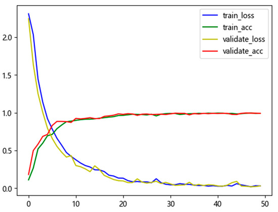
Figure 11.
Loss and accuracy curves for training and validation.
As can be observed from Figure 11, the training set and validation set exhibit consistent trends in loss and accuracy, with their final performances converging toward each other. This demonstrates that the model does not merely memorize the details of the training data verbatim (i.e., no overfitting occurs) while the accuracy continues to improve (i.e., no underfitting exists); instead, it captures the underlying general patterns inherent in the data. Consequently, it can generalize robustly to unseen novel data—that is, the model possesses favorable generalization abilities.
3.2. Analysis of Experimental Results
Rolling bearings, constituting the core components of rotating machinery, critically determine the operational safety and production efficiency of industrial equipment. Under prolonged high-load operation, they are prone to failures such as wear and cracks. Moreover, due to complex influencing factors such as start–stop impacts and load fluctuations during operation, the collected vibration signals often exhibit non-stationary and strongly noisy characteristics. Conventional fault diagnosis methods struggle to accurately extract fault-related features under such conditions, resulting in diagnostic accuracy and real-time performance that are unable to meet practical requirements.
In this study, the VMD technique is first employed to adaptively decompose the vibration signals of bearings, effectively breaking down the complex non-stationary signal into several intrinsic mode functions with physical interpretations. This process successfully separates crucial fault-related information from noise interference. Subsequently, a CNN is applied to extract local features from the temporal sequences of each IMF. Leveraging the local perception and weight-sharing mechanisms of convolutional kernels, the CNN precisely captures localized fault characteristics such as transient impulses and frequency mutations in the vibration signals, thereby enhancing the model’s ability to discern fine-grained fault details. Finally, the multi-head self-attention mechanism from the Transformer architecture is introduced to efficiently capture global dependencies across different modalities and temporal segments through parallel computation in multiple subspaces, enabling the deep integration of multi-scale features.
This integrated approach allows the model to comprehensively uncover latent fault patterns from temporal vibration data, significantly improving the completeness and reliability of fault identification.
Comparative experiments and ablation studies demonstrate that the proposed VMD–CNN–Transformer method outperforms existing mainstream fault diagnosis techniques—such as CNN–Transformer, VMD–CNN, and VMD–Transformer—in terms of diagnostic accuracy and precision for elevator bearing faults. The proposed model attains a diagnostic accuracy of 99.48%, which is markedly superior to that achieved by single or conventional hybrid methods. When handling highly noisy and nonlinear vibration data, the method exhibits outstanding robustness and generalization capabilities, owing to the noise resistance of VMD, the local feature extraction strength of the CNN, and the global contextual modeling ability of the Transformer. This study provides a reliable technical pathway for intelligent fault diagnosis in rolling bearings.
4. Discussion
To address the limitations of traditional methods in extracting features from non-stationary signals and capturing temporal dependencies, this study proposes a fault diagnosis method for rolling bearings based on the VMD–CNN–Transformer model. By integrating the advantages of variational mode decomposition, convolutional neural networks, and Transformer, the proposed approach achieves the efficient extraction of time–frequency features from vibration signals and effectively models global contextual relationships.
The model fully leverages the complementary nature of time domain and frequency domain information through the fusion of temporal and spectral features. Compared to methods that rely solely on either time domain or frequency domain characteristics, this integrated strategy enables the more comprehensive capture of intricate fault patterns, thereby significantly enhancing the model’s robustness against noise and varying operational conditions.
Although the proposed method achieves high diagnostic accuracy, several aspects warrant further improvement:
- (1)
- Generalizability: The current validation of the model remains confined to the publicly available CWRU dataset, and its applicability in real industrial scenarios has yet to be thoroughly verified. To further evaluate the model’s generalization capabilities, performance assessments on additional publicly available datasets from diverse sources should be conducted in future research. Specifically, follow-up studies may incorporate bearing datasets from Jiangnan University (JNU), the University of Connecticut (CU), and the University of Ottawa (OU) for supplementary experiments. Through cross-dataset validation, a more comprehensive examination of the model’s diagnostic stability and adaptability under varying data distributions and operational conditions will be conducted, thereby providing more robust empirical support for its industrial application.
- (2)
- Model Extension: The current research focuses primarily on rolling bearing faults induced by mechanical loads. Nevertheless, in practical industrial scenarios represented by electric vehicles, electrical stress arising from circulating bearing currents also constitutes a critical factor leading to bearing degradation and failure. In future studies, we will consider extending this proposed method to such practical industrial contexts (e.g., electric vehicle-related applications) for further validation and application, thereby broadening its scope of industrial utility beyond the existing mechanical load-centric fault diagnosis framework [27,28].
- (3)
- Model Lightweighting: The computational complexity of the Transformer architecture remains high. Subsequent research could explore lightweight modifications, such as sparse attention mechanisms, to enhance compatibility with embedded systems.
- (4)
- Real-Time Performance: For online monitoring applications, the inference speed of the model requires further optimization to meet industrial standards for real-time fault diagnosis.
5. Conclusions
This study presents a fault diagnosis approach for rolling bearings that integrates variational mode decomposition with deep learning, developing a hybrid VMD-CNN-Transformer model. By leveraging VMD for the adaptive decomposition of non-stationary vibration signals—effectively segregating fault-relevant information from noise interference—employing a convolutional neural network to efficiently extract local features (capturing transient fault impulses and frequency mutations in modal sequences) and utilizing the multi-head self-attention mechanism of the Transformer to capture global dependencies (enabling deep fusion of multi-scale modal features), this approach accomplishes multi-scale feature fusion and fault classification.
The experimental findings demonstrate that this model achieves a fault diagnosis accuracy of 99.48% on the CWRU bearing dataset. In comparison with the existing mainstream fault diagnosis methods validated on the same dataset—including IWOA-VMD-KELM (an approach based on optimized VMD and kernel extreme learning machine), ALA-FMD-MSCA-RN (a feature decomposition and attention-enhanced model oriented toward few-shot learning), and SK-LS-SVM (a method relying on spectral kurtosis for feature extraction and support vector machine)—the proposed VMD-CNN-Transformer model exhibits distinct advantages: it not only outperforms the aforementioned methods in terms of diagnostic accuracy (surpassing them by 0.68%, 2.68%, and 4.48%, respectively), but also possesses more comprehensive feature-mining capabilities for multi-scale modal fusion.
These results fully validate the effectiveness and reliability of the proposed method, which provides a novel technical pathway for the intelligent fault diagnosis of rolling bearings in industrial scenarios characterized by non-stationary signals and intense noise interference.
Author Contributions
Conceptualization, S.W. and F.L.; methodology, S.W., X.S., and J.L.; software, X.S. and J.L.; validation, S.W., X.S., and J.L.; formal analysis, S.W. and F.L.; investigation, Y.R. and X.S.; resources, H.Q.; data curation, X.S.; writing—original draft preparation, S.W., X.S., and J.L.; writing—review and editing, S.W., X.S., J.L., and F.L.; visualization, X.S.; supervision, G.W. and N.S.; project administration, S.W. and M.L.; funding acquisition, G.W. and F.L. All authors have read and agreed to the published version of the manuscript.
Funding
This research was funded in part by the Natural Science Foundation of Henan Province under Grant 252300420380; in part by Henan Provincial Funds for Science and Technology Project under Grants 242102311244, 252102211094, and 252102220021; in part by Henan Provincial Funds for Higher Education Institutions Key Research Project Plan under Grant 24A413005; in part by Henan Provincial Funds for Major Science and Technology Special Project under Grant 251100210200; and in part by Henan Provincial Funds for Key Research and Development Special Project under Grant 251111220600.
Institutional Review Board Statement
Not applicable.
Informed Consent Statement
Not applicable.
Data Availability Statement
The original data presented in this study are openly available via the following platforms: (1) Bearing Data Center of Case Western Reserve University (CWRU): https://engineering.case.edu/bearingdatacenter/download-data-file (accessed on 15 April 2024); (2) GitHub Repository (Mechanical-datasets): https://github.com/cathysiyu/Mechanical-datasets/tree/master/dataset (accessed on 15 April 2024); (3) IEEE DataPort (Vibration Signal Datasets for Bearing Fault Diagnosis and Out-Distribution Detection): https://ieee-dataport.org/documents/vibration-signal-datasets-bearing-fault-diagnosis-and-out-distribution-detection (accessed on 15 April 2024).
Conflicts of Interest
Author Huafei Qian was employed by the company Harbin Shenkong Technology Co., Ltd. The remaining authors declare that the research was conducted in the absence of any commercial or financial relationships that could be construed as a potential conflict of interest.
References
- Xu, F.N.; Ding, N.; Li, N.; Liu, L.; Hou, N.; Xu, N.; Guo, W.; Tian, L.; Xu, H.; Wu, C.-M.L.; et al. A Review of Bearing Failure Modes, Mechanisms and Causes. Eng. Fail. Anal. 2023, 152, 107518. [Google Scholar] [CrossRef]
- Xin, J.; Chen, Y.M.; Wang, L.; Hua, H.L.; Cheng, P. Failure Prediction; Monitoring and Diagnosis Methods for Slewing Bearings of Large-Scale Wind Turbine: A Review. Measurement 2021, 172, 108855. [Google Scholar] [CrossRef]
- He, F.; Xie, G.; Luo, J. Electrical Bearing Failures in Electric Vehicles. Friction 2020, 8, 4–28. [Google Scholar] [CrossRef]
- Zhang, C.; Wei, S.; Dong, G.; Zeng, Y.; Zhu, G.; Zhou, X.; Liu, F. Time-Domain Sparsity Based Bearing Fault Diagnosis Methods Using Pulse Signal-to-Noise Ratio. IEEE Trans. Instrum. Meas. 2024, 73, 3516804. [Google Scholar] [CrossRef]
- Wang, B.; Yang, Q.F. Research on Fault Diagnosis of Industrial Robot Rotating Components Based on Improved Multi-Scale Residual Network. Sci. Technol. Innov. 2024, 7, 217–220. [Google Scholar]
- Elouaham, S.; Dliou, A.; Nassiri, B.; Zougagh, H. Combination Method for Denoising EMG Signals Using EWT and EMD Techniques. In Proceedings of the 2023 IEEE International Conference on Advances in Data-Driven Analytics and Intelligent Systems (ADACIS), Marrakesh, Morocco, 23–25 November 2023; pp. 1–6. [Google Scholar]
- Zheng, L.C.; Liang, X.Y.; Yuan, G.N. Based on Ensemble Neural Network and Improved Extreme Learning Machine for Fault Detection of Mine Mobile Robots. Met. Mine 2024, 6, 159–164. [Google Scholar]
- Cai, J.; Yang, Z.; Liu, X.; Xiong, J.; Chen, H. A Review of Data-Driven Machinery Fault Diagnosis Using Machine Learning Algorithms. J. Vib. Eng. Technol. 2022, 10, 2481–2507. [Google Scholar] [CrossRef]
- Zhong, R.; Hu, B.; Feng, Y.; Lou, S.; Hong, Z.; Wang, F.; Li, G.; Tan, J. Lithium-Ion Battery Remaining Useful Life Prediction: A Federated Learning-Based Approach. Energ. Ecol. Environ. 2024, 9, 549–562. [Google Scholar] [CrossRef]
- Li, Y.; Jia, Z.; Liu, Z.; Shao, H.; Zhao, W.; Liu, Z.; Wang, B. Interpretable Intelligent Fault Diagnosis Strategy for Fixed-Wing UAV Elevator Fault Diagnosis Based on Improved Cross Entropy Loss. Meas. Sci. Technol. 2024, 35, 076110. [Google Scholar] [CrossRef]
- Yuan, B.; Lu, L.; Chen, S. Research on Bearing Fault Diagnosis Based on Vibration Signals and Deep Learning Models. Electronics 2025, 14, 2090. [Google Scholar] [CrossRef]
- Zhong, W.; Pang, B. Intelligent Diagnosis Method for Early Weak Faults Based on Wave Intercorrelation–Convolutional neural networks. Electronics 2025, 14, 2808. [Google Scholar] [CrossRef]
- Wang, H.; Shui, F.; Xie, R.; Gu, J.; Li, C. Few-Shot Bearing Fault Diagnosis Based on ALA-FMD and MSCA-RN. Electronics 2025, 14, 2672. [Google Scholar] [CrossRef]
- Lai, L.; Xu, W.; Song, Z. A Novel Fault Diagnosis Method for Rolling Bearings Based on Spectral Kurtosis and LS-SVM. Electronics 2025, 14, 2790. [Google Scholar] [CrossRef]
- Neupane, D.; Seok, J. Bearing Fault Detection and Diagnosis Using Case Western Reserve University Dataset with Deep Learning Approaches: A Review. IEEE Access 2020, 8, 93155–93178. [Google Scholar] [CrossRef]
- Case Western Reserve University (CWRU) Open-Access Rolling Bearing Dataset. Available online: https://engineering.case.edu/bearingdatacenter/download-data-file (accessed on 15 April 2024).
- Han, F.; Zhang, X.; Cao, J. A Novel Approach of Fault Diagnosis for Gearbox Based on VMD Optimized by GSWOA and Improved RCMSE. Eksploat. I Niezawodn.–Maint. Reliab. 2025, 28. [Google Scholar] [CrossRef]
- Shen, Z.; Shibo, Z.; Bingnan, W.; Thomas, G.H. Deep Learning Algorithms for Bearing Fault Diagnostics—A Comprehensive Review. IEEE Access. 2020, 8, 29857–29881. [Google Scholar]
- You, K.S.; Wang, P.Z.; Huang, P.; Gu, Y.K. A Sound-Vibration Physical-Information Fusion Constraint-Guided Deep Learning Method for Rolling Bearing Fault Diagnosis. Meas. Sci. Technol. 2025, 36, 025103. [Google Scholar]
- Cao, L.; Sun, W. Research on Bearing Fault Identification of Wind Turbines’ Transmission System Based on Wavelet Packet Decomposition and Probabilistic Neural Network. Energies 2024, 17, 2581. [Google Scholar] [CrossRef]
- Chen, L.; Zhang, X.; Li, Z.; Jiang, H. Research on a Wind Turbine Gearbox Fault Diagnosis Method Using Singular Value Decomposition and Graph Fourier Transform. Sensors 2024, 24, 3234. [Google Scholar] [CrossRef]
- Yan, R.; Lin, J. Equipment Intelligent Operation and Maintenance; CRC Press: Boca Raton, FL, USA, 2025. [Google Scholar] [CrossRef]
- Wang, C.; Tian, X.; Zhou, F.; Shao, X.; Liang, X.; Li, H. Fault Diagnosis of Electric Transmission System Based on Graph-Enhanced Deep Feature Fusion Network Model Using Efficient Decision Mapping. Meas. Sci. Technol. 2025, 36, 046123. [Google Scholar] [CrossRef]
- Vaswani, A.; Shazeer, N.; Parmar, N.; Uszkoreit, J.; Jones, L.; Gomez, A.N.; Kaiser, Ł.; Polosukhin, I. Attention Is All You Need. In Proceedings of the 31st Conference on Neural Information Processing Systems (NIPS’17), Long Beach, CA, USA, 4–9 December 2017; pp. 6000–6010. [Google Scholar]
- Jin, D.; He, C.; Zou, Q.; Qin, Y.; Wang, B. Source Code Vulnerability Detection Based on Joint Graph and Multimodal Feature-Fusion. Electronics 2025, 14, 975. [Google Scholar] [CrossRef]
- Al-Karawi, A.; Abofanas, M.; Mohammedqasem, R.; Mohammedqasim, H. Revolutionizing the Classification of Medical Image Classification by Using Integrating Advanced Neural Networks with Pre-Processing. Procedia Comput. Sci. 2025, 258, 1326–1337. [Google Scholar] [CrossRef]
- Tombul, Y.; Tillmann, P.; Andert, J. Simulation of the Circulating Bearing Currents for Different Stator Designs of Electric Traction Machines. Machines 2023, 11, 811. [Google Scholar] [CrossRef]
- Jie, H.; Wang, C.; See, K.Y.; Li, H.; Zhao, Z. A Systematic EV Bearing Degradation Testing Approach Considering Circulating Bearing Currents. IEEE/ASME Trans. Mechatron. 2025. [Google Scholar] [CrossRef]
Disclaimer/Publisher’s Note: The statements, opinions and data contained in all publications are solely those of the individual author(s) and contributor(s) and not of MDPI and/or the editor(s). MDPI and/or the editor(s) disclaim responsibility for any injury to people or property resulting from any ideas, methods, instructions or products referred to in the content. |
© 2025 by the authors. Licensee MDPI, Basel, Switzerland. This article is an open access article distributed under the terms and conditions of the Creative Commons Attribution (CC BY) license (https://creativecommons.org/licenses/by/4.0/).