Article

Learning Human–Robot Proxemics Models from Experimental Data

1
COSY@Home-Lab, Faculty of Technology, Bielefeld University, 33615 Bielefeld, Germany
2
Neuro-Information Technology, Otto-von-Guericke-University Magdeburg, 39106 Magdeburg, Germany
*
Author to whom correspondence should be addressed.
Electronics 2025, 14(18), 3704; https://doi.org/10.3390/electronics14183704
Submission received: 30 July 2025 / Revised: 13 September 2025 / Accepted: 16 September 2025 / Published: 18 September 2025
(This article belongs to the Special Issue Human Robot Interaction: Techniques, Applications, and Future Trends)

Abstract

Humans in a society generally tend to implicitly adhere to the shared social norms established within that culture. Robots operating in a dynamic environment shared with humans are also expected to behave socially to improve their interaction and enhance their likability among humans. Especially when moving into close proximity of their human partners, robots should convey perceived safety and intelligence. In this work, we model human proxemics as robot navigation costs, allowing the robot to exhibit avoidance behavior around humans or to initiate interactions when engagement is required. The proxemic model enhances robot navigation by incorporating human-aware behaviors, treating humans not as mere obstacles but as social agents with personal space preferences. The model of interaction positions estimates suitable locations relative to the target person for the robot to approach when an engagement occurs. Our evaluation on human–robot interaction data and simulation experiments demonstrates the effectiveness of the proposed models in guiding the robot’s avoidance and approaching behaviors toward humans.

1. Introduction

Proxemics [1] is the study of human spatial behavior and the use of space, particularly the distances maintained between individuals. In shared space, people tend to unconsciously structure interpersonal space, maintaining varying distances based on social relationships such as families, friends, and strangers. Hall et al. [1] propose intimate, personal, social, and public zones. For instance, if an acquaintance enters the intimate zone, it often results in discomfort. These proxemic zones are typically represented as concentric circles with fixed radii (intimate zone: 0–0.45 m, personal zone: 0.45–1.2 m, social zone: 1.2–3.6 m, and public zone: 3.6–7.6 m) [1]. Further studies revealed that more frontal space is required, possibly due to actions performed in the frontal direction [2]. This forms zones of an egg shape [2]. Conversely, it was found that people tend to have more space behind them in an approaching scenario because the visual inability to see the back brings about a greater sense of insecurity [2]. These two opposite results indicate that preferences of space differ individually. In addition, a left–right asymmetry in proxemic zones is investigated, revealing that people tend to keep less space from obstacles on the side of their dominant hand [2]. Furthermore, people from different cultures do not share common distance sensing [1,3]. For instance, Germans tend to maintain a larger interpersonal distance than Arabs in a multi-person conversation [4].
In social interactions involving two or more individuals, such as standing conversations, the concept of F-formation [5] has been introduced to describe the spatial organization of participants. Typical F-formation configurations include dyadic groups positioned face-to-face (vis-à-vis), side-by-side, or at approximately a 90-degree angle (L-shape), as well as groups of three or more people arranged in a circle (Circle) [6].
Robots are also expected to behave in a human-like manner in dynamic environments shared with people. User studies [3,4] prove that proxemics conventions between people are also applicable to human–robot interactions. Therefore, we introduce a human proxemic model, an interaction position model, and propose a learning method that enables adaptation to diverse preferences in space usage, thereby equipping robots with social knowledge and facilitating socially aware human–robot coexistence. We categorize spatial behavior in human–robot coexistence into avoidance behaviors that prevent interference and approach behaviors that enable interaction. The proxemic model learns human proxemic behavior from human–human avoidance data and is further integrated into the social cost layer of the robot’s navigation system. The interaction position model estimates high-probability interaction locations near the target person, allowing the robot to select an optimal position for initiating interaction.

2. Related Work

2.1. Empirical Studies

Empirical studies on human–robot proxemics (HRP) [7] validate hypotheses proposed about their interactions in close proximity by conducting experiments with participants. First, it has been found that proxemic-aware agents are perceived as significantly more anthropomorphic and trustworthy [8,9]. Second, human proxemic preferences evolve over time as users interact with the robot [10]. Notably, prior experience with pets or interaction with robots shows a reduction of the personal space that individuals maintain around robots [11]. Moreover, the influences of robot gaze were also investigated; ref. [8] stated that robot gaze behavior does not significantly affect humans’ perception of the robot’s social presence and emotional state, while ref. [11] found that robot gaze influences proxemic behavior such that the distance a human maintains from the robot changes.
Samarakoon et al. [7] summarized the factors affecting human–robot proxemics (HRP), including user attributes, robot attributes, and context/environment. While human proxemics explicitly and directly depends on body pose, it is also implicitly influenced by identity factors such as gender, age, personality, and culture [7]. Robot attributes include speed, gaze direction, and robot hardware-related factors, such as height, appearance, noise level, voice type, and vocal and facial emotions [7]. Given that human proxemic behavior varies across individuals and over time, the development of our adaptive learning method is essential to effectively accommodate these variations. Moreover, although this work focuses on mobile service robots, our proposed learning framework also enables fine-tuning across different robot platforms.

2.2. Modeling of Proxemics

Kirby R. [12] modeled human proxemics using an asymmetric Gaussian integral function based on the human position and rotation. The asymmetry is modeled by defining distinct variance parameters for the facing direction, sides, and rear; ref. [13] applied a skew normal distribution SN [14,15] to create various interpersonal spaces, taking into account the human’s position, orientation, and the dominant side. However, these proxemic models rely on fixed, manually defined parameters, and consequently fail to capture the fact that proxemic behavior differs among individuals and evolves over time.
The Social Force Model [16] includes acceleration of the human, repulsive effects, and attractive effects from the environment to model the movements of humans in a crowd; ref. [17] integrated a collision prediction-based Social Force Model (CP-SFM) into a social navigation framework as the local planner, but it is highly dependent on the model parameters and can become stuck in the local minima when the repulsive and attractive forces are equal and cancel each other out.
Patompak et al. [18] extended the Social Force Model by incorporating a fuzzy system with Gaussian membership functions, in which the Gaussian function centers are adaptively tuned via R-learning. The approaches [19,20] using reinforcement learning (RL) train agents to navigate in a socially proxemic manner by integrating the social proxemic norms into the reward function or as a penalty term. By contrast, inverse reinforcement learning (IRL) [21] does not define the reward manually but learns the reward/cost function from expert demonstrations; [22] learned an optimal reward function from human trajectory observations such that the robot’s policy reproduces human-like behavior.
Eirale et al. [23] learned a social costmap from goal and people positions using an encoder–decoder neural network and validated it in two example scenarios: people queuing and people conversing in small groups. However, proxemics is not explicitly taken into account, and the robot’s navigation goal must be provided.
Therefore, to address the research gap in previous work, we explicitly learn proxemic zones using the skew normal distribution SN from experimental data rather than manually defining model parameters as in prior approaches. Compared to normal/Gaussian distributions, the skew normal distribution SN introduces skewness, which allows for asymmetry. For example, in two-dimensional cases, the normal distribution can only be circular or elliptical, while the skew normal distribution SN also produces a variety of distorted, asymmetric elliptical shapes, determined by the parameters of skewness and covariance. Since the proxemic zones could exhibit left–right asymmetry due to hand dominance and front–back asymmetry due to eye vision, our learnable approach with the skew normal distribution SN is capable of modeling these variations in shape. In addition, we estimate the density of interaction positions around the target person to propose a navigation goal for the robot when initiating an interaction.

3. Method

3.1. Data Preparation

Dataset. We used a public dataset of human–robot approach behaviors: CongreG8 [24]. In this dataset, a human or a pepper robot [25] firstly walks around a conversational group of three persons and then attempts to join the group. All participants, including humans and the robot, are tracked using a motion capture system. Forty human participants are divided into ten groups, four of which also interact with a robot participant. The robot was remotely controlled by an operator using the Wizard of Oz (WoZ) method, allowing human participants to perceive it as fully autonomous. We used the data from human-only groups (four humans) as training data and the data from robot groups (three humans and one robot) as test data.
Data Processing. In the CongreG8 dataset [24], the position and the orientation T p of every person are captured in the global reference frame world , which is the coordinate system of the motion capture system. The relative poses are then computed by homogeneous transformation:
T p 1 p 2 = T p 1 World · T World p 2 = T World p 1 1 · T World p 2
where T p 1 p 2 refers to the p 2 pose of person 2 relative to person 1, and T World p 1 and T World p 2 indicate the poses of person 1 and person 2 in the world, respectively. We computed relative chest poses for every participant with respect to each other in the group.
The sequential data are roughly divided into two stages: the avoidance stage, when the newcomer walks outside the conversational group, and the interaction stage, when the newcomer joins the group and begins interacting with other members. The trajectories when the newcomer avoids the conversational group are used to learn the proxemic model. The endpoint of each trajectory is assumed to represent the final interaction position where the newcomer has already joined the group.

3.2. Proxemic Model

We deploy the probability density function (PDF) of the bivariate skew normal distribution [14]:
f ( x ) = 2 · ϕ 2 ( x ; μ , Σ ) · Φ α Σ 1 2 ( x μ )
where x R 2 represents X , Y world coordinates in space. ϕ 2 ( · ; μ , Σ ) is the PDF of the bivariate normal distribution with mean μ and covariance matrix Σ . Φ ( · ) is the standard normal CDF. The skewness α R 2 controls the shape of the distribution.
The yaw of the human R y a w is further integrated:
μ ˜ = R y a w · μ + p α ˜ = R y a w · α · R y a w T Σ ˜ = R y a w · Σ
where p denotes the human position. The position and the yaw of human p , R y a w are parameters being perceived. α , μ , Σ are learnable parameters to build the proxemic zones.
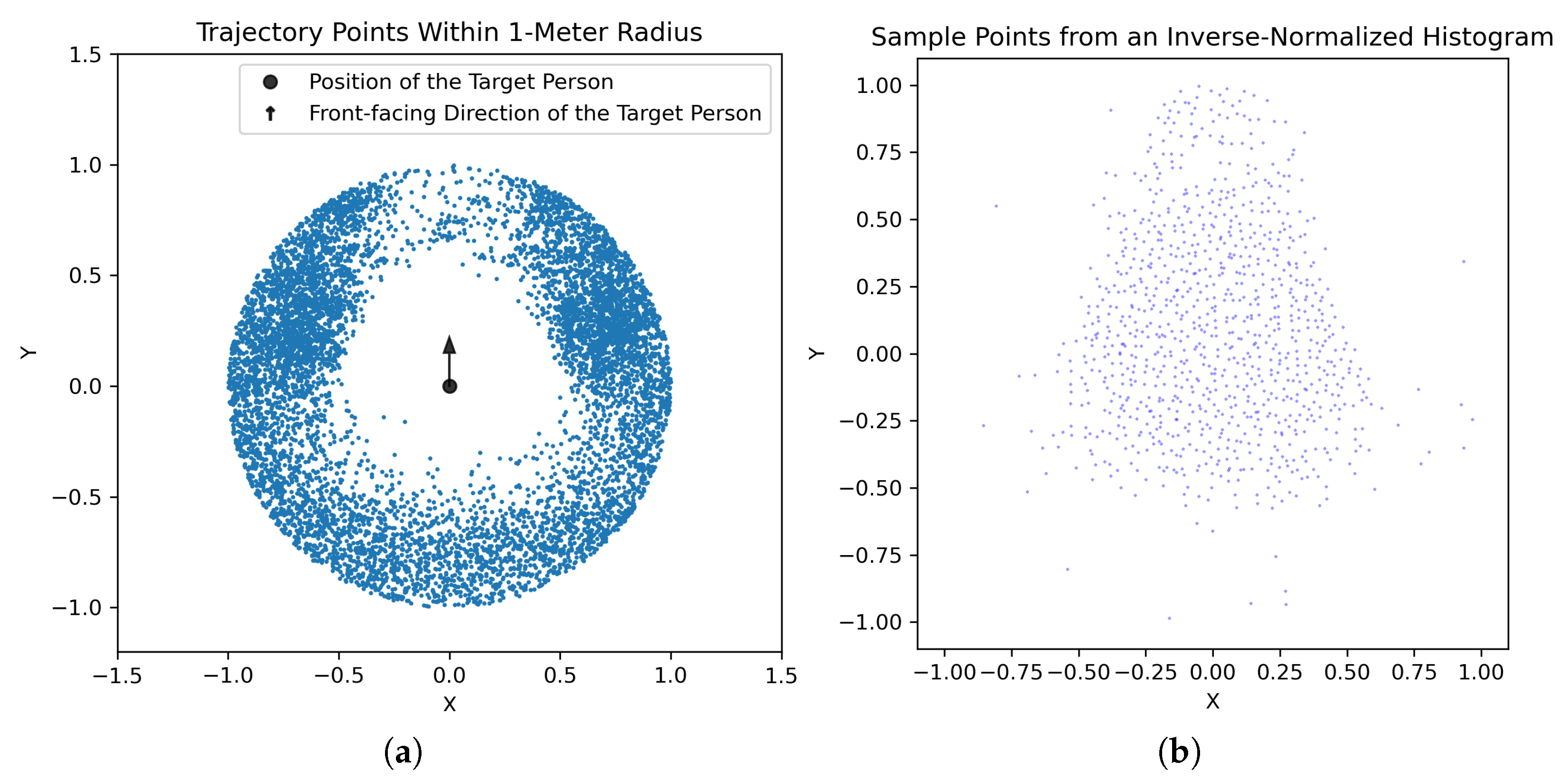
Given the processed avoidance trajectories of the human groups with respect to a target individual, we observed an egg-shaped empty region without trajectory points, as illustrated in Figure 1a. This indicates that the area is not intended to be entered. In order to model that shape, we first create a 2D histogram H from the relative trajectory points D = { ( x n , y n ) } n = 1 N R 2 :
H i , j = n = 1 N δ x j min x n < x j max · δ y i min y n < y i max
where
δ ( condition ) = 1 if condition is true 0 otherwise
The boundaries of bin ( i , j ) are given by:
x j min = r + j Δ , x j max = r + ( j + 1 ) Δ
y i min = r + i Δ , y i max = r + ( i + 1 ) Δ
Here, the region [ r , r ] × [ r , r ] is uniformly partitioned into B × B bins, each of side length
Δ = 2 r B
where the radius r of the region is defined to be 1 m. The area within a 1-m radius around a person is commonly considered to be the personal space. B is set to 60, resulting in a bin side length of 0.33 m.
Second, an inverse-normalized histogram is computed as
H i , j inv = H max H i , j H max
This transformation assigns low values to dense regions and high values to sparse regions. Areas without trajectory points indicate regions that should not be intruded upon, implying high costs for intrusion. A higher density of trajectory points within a region indicates greater accessibility. Consequently, the navigation cost for the robot should be reduced accordingly.
Third, sample points are uniformly drawn from each bin H i , j inv in proportion to its density, as shown in Figure 1b. Finally, the expectation maximization (EM) algorithm [26,27] is applied to these sample points to estimate the parameters of the skew normal density function.
Figure 1. Data preparation for the proxemic model. (a) Trajectory points of other individuals relative to the target person. (b) Sample points after inversing and normalizing the data from (a).
Electronics 14 03704 g001

3.3. Model of Interaction Positions

We estimate the densities of interaction positions using a non-parametric method, kernel density estimation (KDE) [28], based on the processed relative endpoints of trajectories x 1 , x 2 , , x n R 2 plotted in Figure 2a.The estimate at any point x R 2 is given by [29]:
ρ ^ h ( x ) = 1 n h 2 i = 1 n K x x i h
where h = 0.15 is the bandwidth that controls smoothing, and K : R 2 R denotes the kernel function, and we chose the Gaussian kernel.

4. Results

4.1. Proxemic Model

The learned human proxemic model is applied to individuals, as illustrated in Figure 3a, where the heading direction is defined as zero yaw angle. The density values of the learned model represent the navigation costs of reaching specific positions relative to the target person. In the case of a group interaction shown in Figure 3b, the individual proxemic model is scaled into a mixture model representing multi-person interactions involving three individuals. This enables the newcomer to approach along a path with the lowest overall mixture costs, ensuring that all group members feel comfortable.

4.2. Model of Interaction Positions

The KDE model [29] is fitted to the data on interaction positions with respect to the target person presented in Figure 2a. Figure 2b presents the fitted density map, where each density value reflects the suitability of a given location as an interaction position.

5. Evaluation

5.1. Experimental Setup

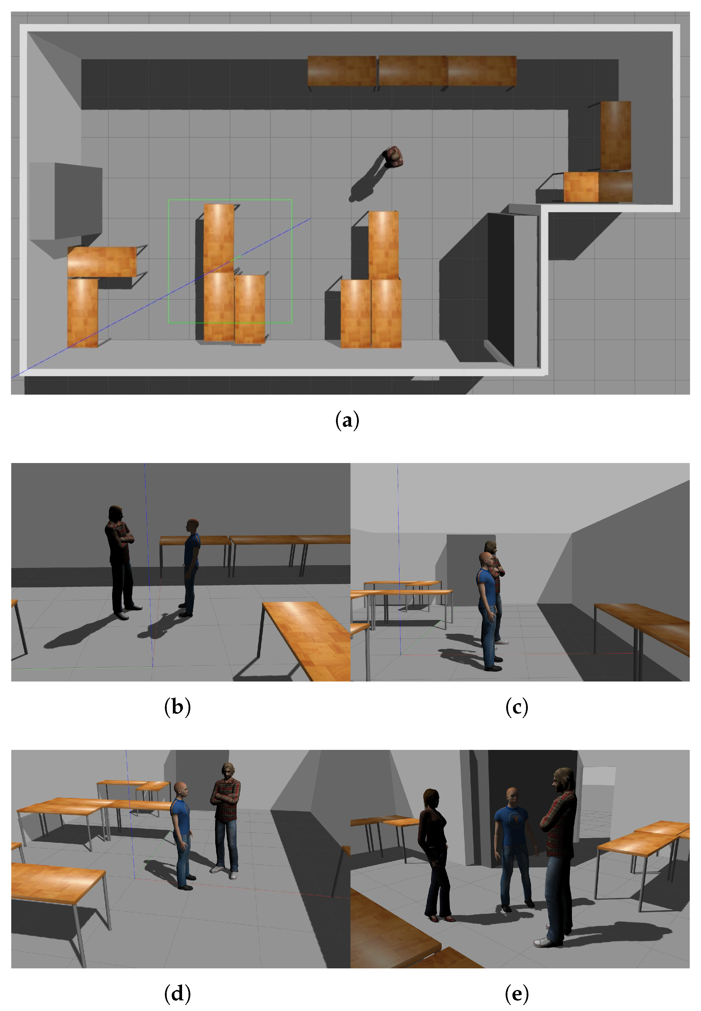
A simulation of human avatars and a mobile robot, Tiago [30], was created in Gazebo [31]. The environment is a 13 × 7 m room with obstacles such as walls and furniture, as depicted in Figure 4a. The scenarios comprise a single individual and social groups of two or three people. The simulation of human social groups follows the F-formation configurations [5,6], which cover face-to-face, side-by-side, L-shape, and circle, as visualized in Figure 4b–e.
For each trial, the robot’s pose was initialized randomly within the open space surrounding the crowd, and it was tasked with either avoiding or joining the crowd. In the avoidance condition, the robot’s goal position was set across the crowd, directly opposite its initial position, to elicit avoidance. In the approach condition, the goal position was determined according to the interaction position model.
Ten participants (five female and five male) were invited to view simulation videos recorded from a third-person perspective positioned near the human crowd in order to assess the robot’s likability, perceived intelligence, and perceived safety during avoidance and approach behaviors.

5.2. Proxemic Model

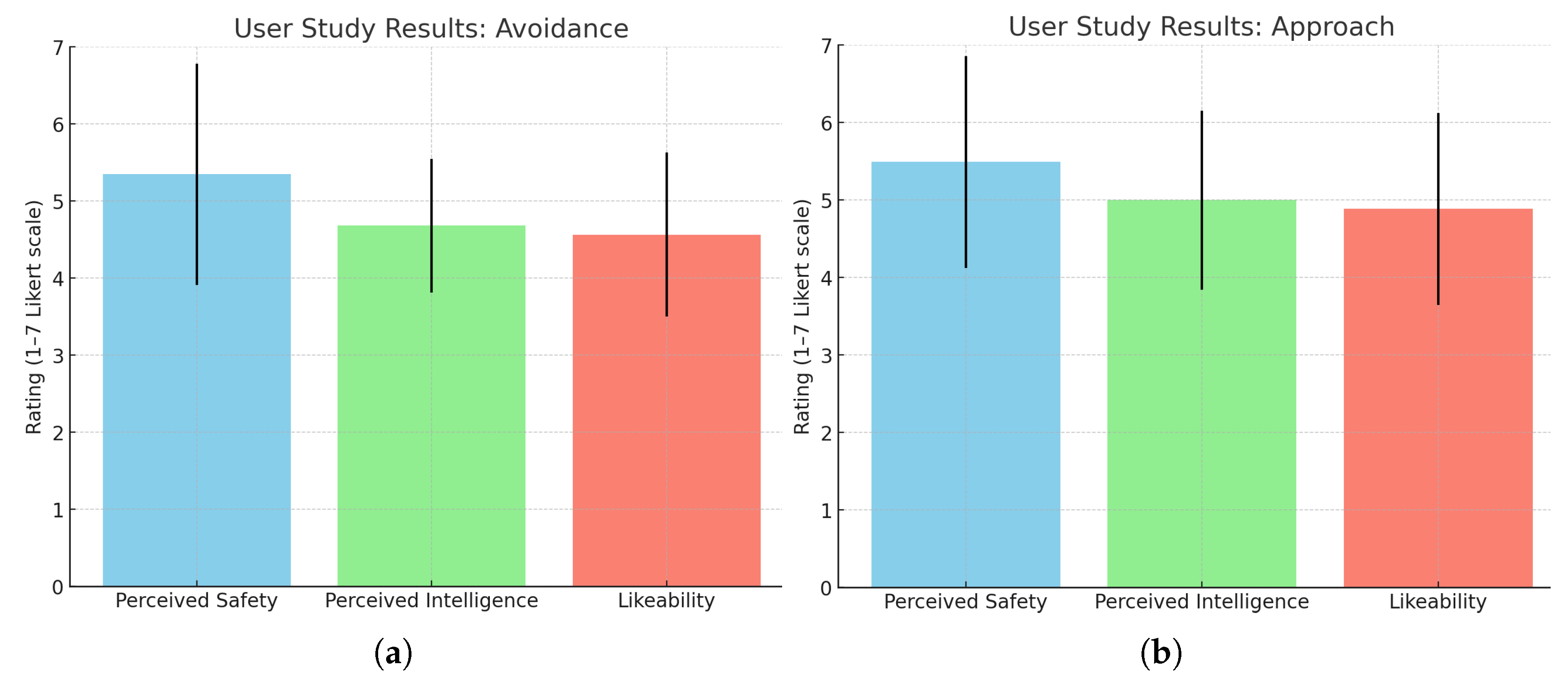
Our learned proxemic model is applied to each individual as a social cost layer in robot navigation. An illustrative example is shown in Figure 5a. With the social layer, Tiago respects the three persons as a group and drives around them. In contrast, when treating the humans only as obstacles, Tiago passes through the group to reach its destination (Figure 5b,d). Moreover, Figure 6a presents the mean ratings of participants on the three dimensions (perceived safety, perceived intelligence, and likeability) for the robot’s avoidance behaviors. Overall, participants evaluated the robot positively. These results validate the effectiveness of our learned proxemic model for robot navigation in environments shared with humans.
In addition, the proxemic costs of the robot’s navigation are evaluated using the test data from the robot groups in the CongreG8 dataset [24]. During the robot’s avoidance phase, a low or zero cost is expected when there is no intention of interaction between the human and the robot. Since no complete user interaction satisfaction questionnaire for the test data could be found online in the dataset, third-party manual observation was employed to assess the behavior of the teleoperated robot.
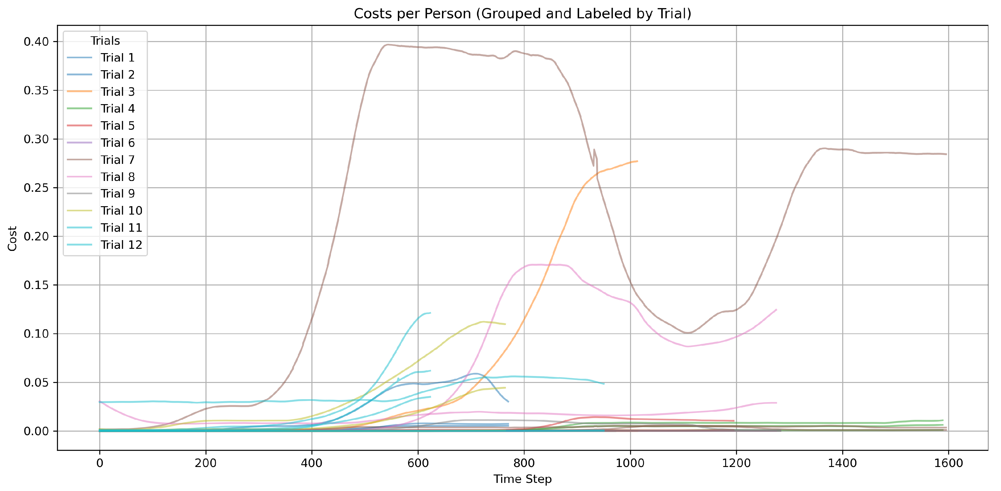
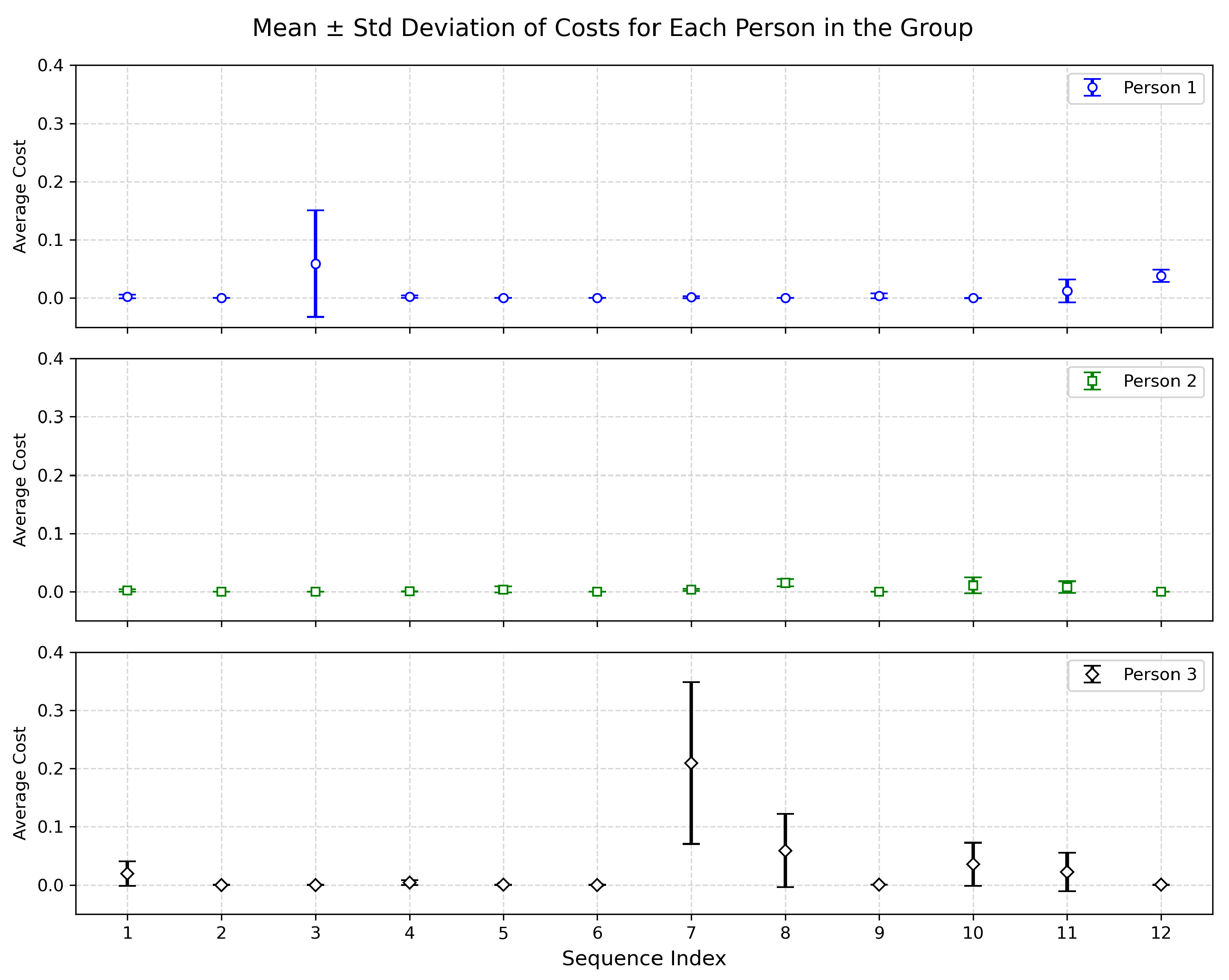
Figure 7 plots the proxemic costs over time produced by the proxemic model. The average cost and its standard deviation are further evaluated, as presented in Figure 8. Most of the costs lie within the range of 0 to 0.05, which is also reflected in the average. In the final phase of the trajectories, the costs of Trials 10 and 12 rise above 0.1 and the cost of Trial 3 exceeds 0.25. This is because the newcomer approaches the group in a relatively suboptimal path. As illustrated in Figure 9, the robot joins the group from a side close to one of the group members, rather than approaching from the center of the free space. Furthermore, in Trial 8, an individual in the group moves closer to the center of the group and then returns to the original position, resulting in a slight increase in cost beyond 0.15, followed by a subsequent decrease. In addition, the cost of Trial 7 exhibits a relatively large standard deviation, and it first increases, then drops, and subsequently rises again. This fluctuation results from the robot initially approaching the group, briefly withdrawing, and then re-approaching.
We also evaluated the asymmetric Gaussian model [12] on the test data as a baseline. The parameters of the model are defined and given in [12]. Figure 10 displays the cost curves of robot navigation generated by this model. The cost values range from approximately 0.1 to 0.9. The majority of the curves show an increasing trend. However, it is not straightforward to interpret which cost levels correspond to poor avoidance behavior. In comparison with this baseline model, our model with learned parameters yields discriminative cost values for effective avoidance behavior and personal space intrusion. Moreover, our resulting proxemic cost values can be directly integrated into the robot’s navigation system as a social layer [32].

5.3. Model of Interaction Positions

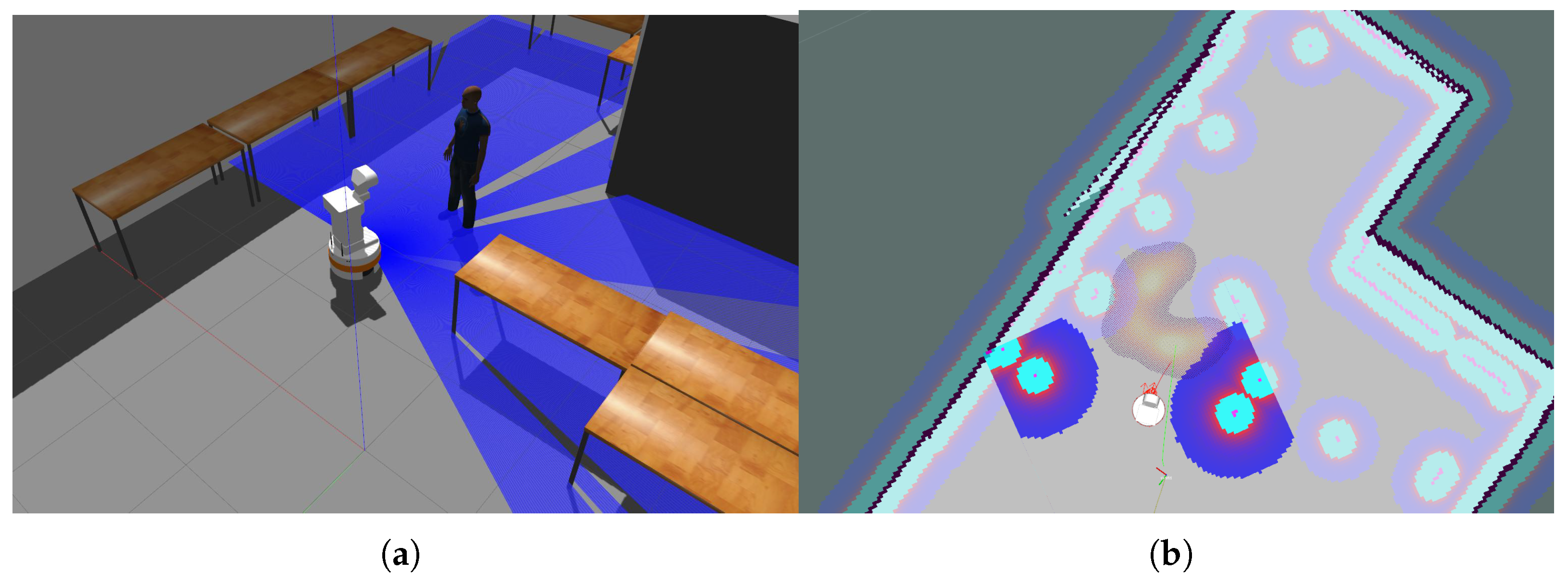
Our model of interaction positions is applied to robot navigation to select a navigation goal when the engagement between the robot and the human occurs. Specifically, our learned KDE model estimates densities around the interacting individual based on their position and yaw. Figure 11a shows the position selected by the robot to initiate interaction with the human, and Figure 11b visualizes the planned robot path together with the applied interaction position model. Additionally, Figure 6b presents the mean ratings of participants for the robot’s approach behaviors in the user study.
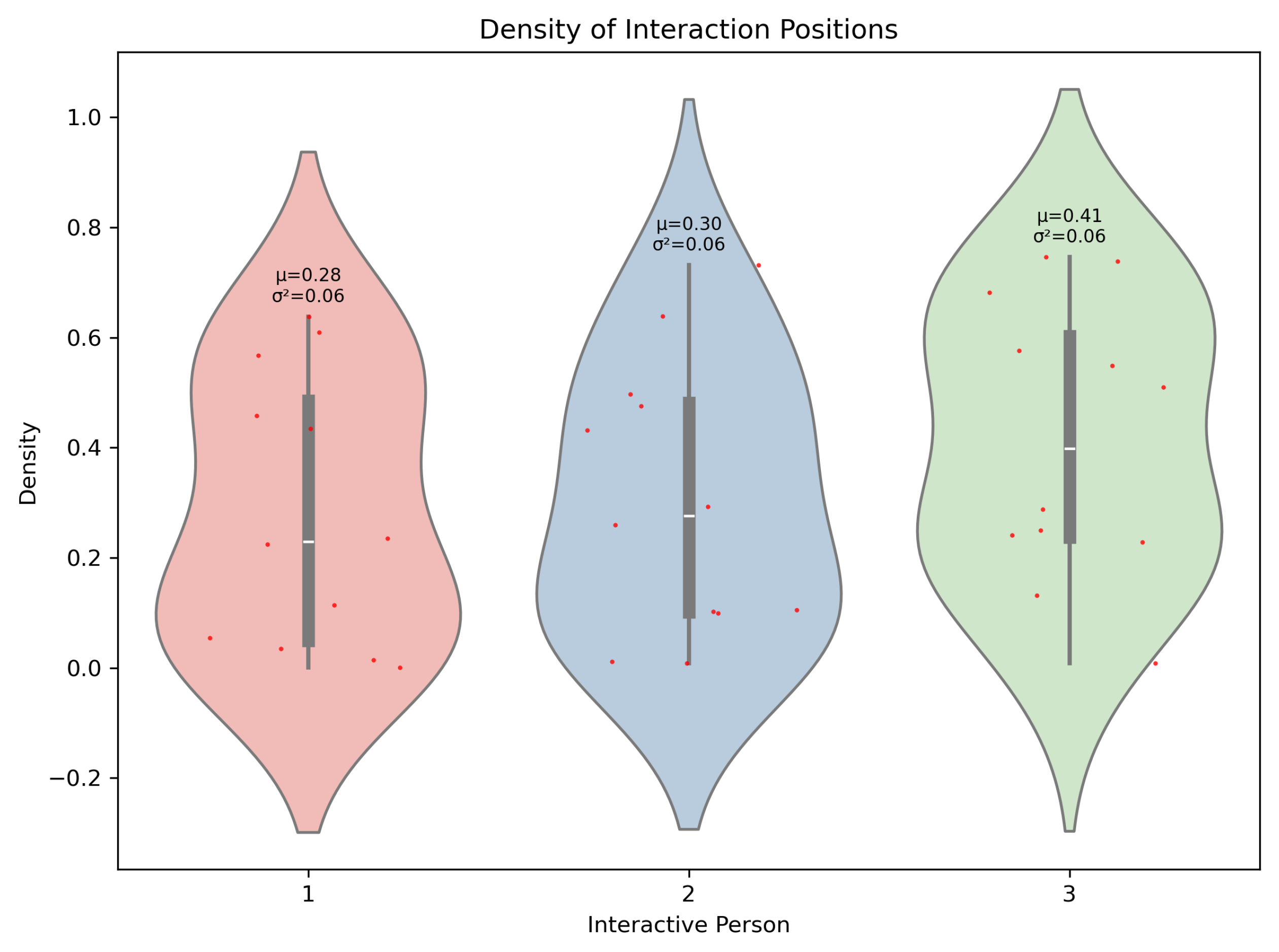
Furthermore, the densities of the robot’s interaction positions in the test data of the CongreG8 dataset [24] are estimated using the fitted KDE model. Figure 12 illustrates the distribution of interaction position densities for each of the three interacting individuals. Most interaction positions are located in regions where the density is greater than zero. In the group interaction involving three other individuals, the results show higher density values for one member compared to the others.

6. Discussion

Our proxemic model is created based on the human body pose and can be applied to individuals within a group by forming a mixture model. However, other modalities, such as head pose and gaze direction, can also affect human spatial behaviors. Our model may be extended to a multimodal mixture model by incorporating these additional social cues for each individual. Moreover, since human proxemic behaviors differ individually, a personalized model can be learned for each individual given sufficient data.

7. Conclusions

In conclusion, this work proposes a learning approach to identify human proxemic preferences for socially aware robot navigation. The learned proxemic model maps human proxemic zones into social costs, and it is scalable to multi-person interaction scenarios. The interaction position model determines socially appropriate locations in the vicinity of the target person for an agent to proactively initiate interaction. The identified location is subsequently designated as a navigation goal, upon which the robot computes a trajectory that minimizes the proxemic cost by incorporating the proxemic model. Our results show the effectiveness of guiding the robot to avoid a group in compliance with human proxemic conventions and approach a human for interaction. In the future, it would be beneficial to fine-tune the model parameters online to enable personalized adaptation for individual users.

Author Contributions

Conceptualization, Q.Y. and S.W.; methodology, Q.Y.; software, L.K. and Q.Y.; validation, Q.Y.; formal analysis, Q.Y. and L.K.; investigation, L.K. and M.J.; data curation, L.K.; writing—original draft preparation, Q.Y.; writing—review and editing, S.W.; visualization, Q.Y.; supervision, S.W. and A.A.-H.; project administration, S.W. and A.A.-H.; funding acquisition, S.W. All authors have read and agreed to the published version of the manuscript.

Funding

This work is funded by Deutsche Forschungsgemeinschaft (DFG, German Research Foundation) under grant number 502483052.

Data Availability Statement

The original contributions presented in this study are included in the article. Further inquiries can be directed to the corresponding author. Code is publicly available at https://github.com/Q-Y-Yang/human-robot-proxemics-models, accessed on 16 September 2025.

Conflicts of Interest

The authors declare no conflicts of interest.

Abbreviations

The following abbreviations are used in this manuscript:
HRPHuman–Robot Proxemics
SN Skew Normal Distribution
SFMSocial Force Model
RLReinforcement Learning
IRLInverse Reinforcement Learning
WoZWizard of Oz
PDFProbability Density Function
EMExpectation Maximization
KDEKernal Density Estimation

References

  1. Hall, E.T.; Birdwhistell, R.L.; Bock, B.; Bohannan, P.; Diebold, A.R.; Durbin, M.; Edmonson, M.S.; Fischer, J.L.; Hymes, D.; Kimball, S.T.; et al. Proxemics [and Comments and Replies]. Curr. Anthropol. 1968, 9, 83–108. [Google Scholar] [CrossRef]
  2. Neggers, M.; Cuijpers, R.; Ruijten, P.; IJsselsteijn, W. Determining Shape and Size of Personal Space of a Human when Passed by a Robot. Int. J. Soc. Robot. 2022, 14, 561–572. [Google Scholar] [CrossRef]
  3. Wang, L.; Rau, P.L.P.; Evers, V.; Robinson, B.K.; Hinds, P. When in Rome: The role of culture & context in adherence to robot recommendations. In Proceedings of the 5th ACM/IEEE International Conference on Human-Robot Interaction, Osaka, Japan, 2–5 March 2010; pp. 359–366. [Google Scholar]
  4. Eresha, G.; Häring, M.; Endrass, B.; André, E.; Obaid, M. Investigating the Influence of Culture on Proxemic Behaviors for Humanoid Robots. In Proceedings of the International Symposium on Robot and Human Interactive Communication (RO-MAN 2013), Gyeongju, Republic of Korea, 26–29 August 2013; pp. 430–435. [Google Scholar]
  5. Kendon, A. Conducting Interaction: Patterns of Behavior in Focused Encounters; Studies in Interactional Sociolinguistics; Cambridge University Press: Cambridge, UK, 1990. [Google Scholar]
  6. Cristani, M.; Paggetti, G.; Vinciarelli, A.; Bazzani, L.; Menegaz, G.; Murino, V. Towards Computational Proxemics: Inferring Social Relations from Interpersonal Distances. In Proceedings of the Third International Conference on Privacy, Security, Risk and Trust and 2011 IEEE Third International Conference on Social Computing, Boston, MA, USA, 9–11 October 2011; pp. 290–297. [Google Scholar] [CrossRef]
  7. Samarakoon, S.M.B.P.; Muthugala, M.A.V.J.; Jayasekara, A.G.B.P. A Review on Human–Robot Proxemics. Electronics 2022, 11, 2490. [Google Scholar] [CrossRef]
  8. Fiore, S.M.; Wiltshire, T.J.; Lobato, E.J.; Jentsch, F.G.; Huang, W.H.; Axelrod, B. Toward understanding social cues and signals in human–robot interaction: Effects of robot gaze and proxemic behavior. Front. Psychol. 2013, 4, 859. [Google Scholar] [CrossRef] [PubMed]
  9. Petrak, B.; Weitz, K.; Aslan, I.; André, E. Let me show you your new home: Studying the effect of proxemic-awareness of robots on users’ first impressions. In Proceedings of the The 28th IEEE International Conference on Robot & Human Interactive Communication, New Delhi, India, 14–18 October 2019. [Google Scholar]
  10. Mead, R.; Matarić, M.J. Robots have needs too: How and why people adapt their proxemic behavior to improve robot social signal understanding. J. Hum.-Robot Interact. 2016, 5, 48–68. [Google Scholar] [CrossRef]
  11. Takayama, L.; Pantofaru, C. Influences on proxemic behaviors in human-robot interaction. In Proceedings of the 2009 IEEE/RSJ International Conference on Intelligent Robots and Systems, St. Louis, MO, USA, 10–15 October 2009; pp. 5495–5502. [Google Scholar] [CrossRef]
  12. Kirby, R. Social Robot Navigation. Ph.D. Thesis, Carnegie Mellon University, Pittsburgh, PA, USA, 2010. [Google Scholar]
  13. Papadakis, P.; Rives, P.; Spalanzani, A. Adaptive spacing in human-robot interactions. In Proceedings of the 2014 IEEE/RSJ International Conference on Intelligent Robots and Systems, Chicago, IL, USA, 14–18 September 2014; pp. 2627–2632. [Google Scholar] [CrossRef]
  14. Azzalini, A.; Valle, A.D. The Multivariate Skew-Normal Distribution. Biometrika 1996, 83, 715–726. [Google Scholar] [CrossRef]
  15. Azzalini, A.; Capitanio, A. Statistical Applications of the Multivariate Skew Normal Distribution. J. R. Stat. Soc. Ser. B Stat. Methodol. 1999, 61, 579–602. [Google Scholar] [CrossRef]
  16. Helbing, D.; Molnár, P. Social force model for pedestrian dynamics. Phys. Rev. E 1995, 51, 4282–4286. [Google Scholar] [CrossRef] [PubMed]
  17. Kivrak, H.; Cakmak, F.; Kose, H.; Yavuz, S. Social navigation framework for assistive robots in human inhabited unknown environments. Eng. Sci. Technol. Int. J. 2021, 24, 284–298. [Google Scholar] [CrossRef]
  18. Patompak, P.; Jeong, S.; Nilkhamhang, I.; Chong, N. Learning Proxemics for Personalized Human–Robot Social Interaction. Int. J. Soc. Robot. 2020, 12, 267–280. [Google Scholar] [CrossRef]
  19. Millán-Arias, C.; Fernandes, B.; Cruz, F. Proxemic behavior in navigation tasks using reinforcement learning. Neural Comput. Appl. 2022, 35, 16723–16738. [Google Scholar] [CrossRef]
  20. Chen, Y.F.; Everett, M.; Liu, M.; How, J.P. Socially aware motion planning with deep reinforcement learning. In Proceedings of the 2017 IEEE/RSJ International Conference on Intelligent Robots and Systems (IROS), Vancouver, BC, Canada, 24–28 September 2017; pp. 1343–1350. [Google Scholar] [CrossRef]
  21. Abbeel, P.; Ng, A.Y. Apprenticeship learning via inverse reinforcement learning. In Proceedings of the Twenty-First International Conference on Machine Learning (ICML), Banff, AB, Canada, 4–8 July 2004; p. 1. [Google Scholar]
  22. Baghi, B.H.; Dudek, G. Sample Efficient Social Navigation Using Inverse Reinforcement Learning. arXiv 2021, arXiv:2106.10318. [Google Scholar] [CrossRef]
  23. Eirale, A.; Leonetti, M.; Chiaberge, M. Learning Social Cost Functions for Human-Aware Path Planning. In Proceedings of the 2024 IEEE/RSJ International Conference on Intelligent Robots and Systems (IROS), Abu Dhabi, United Arab Emirates, 14–18 October 2024; pp. 5364–5371. [Google Scholar] [CrossRef]
  24. Yang, F.; Gao, A.Y.; Ma, R.; Zojaji, S.; Castellano, G.; Peters, C. A dataset of human and robot approach behaviors into small free-standing conversational groups. PLoS ONE 2021, 16, e0247364. [Google Scholar] [CrossRef]
  25. SoftBank Robotics Group. Pepper Robot. Available online: https://aldebaran.com/en/pepper/ (accessed on 4 September 2025).
  26. Dempster, A.; Laird, N.; Rubin, D. Maximum likelihood from incomplete data via the EM algorithm. J. R. Stat. Soc. Ser. B 1977, 39, 1–38. [Google Scholar] [CrossRef]
  27. Kulkarni, K. mvem: Maximum Likelihood Parameter Estimation in Multivariate Distributions Using EM Algorithms. Available online: https://github.com/krisskul/mvem (accessed on 15 September 2025).
  28. Parzen, E. On estimation of a probability density function and mode. Ann. Math. Stat. 1962, 33, 1065–1076. [Google Scholar] [CrossRef]
  29. Pedregosa, F.; Varoquaux, G.; Gramfort, A.; Michel, V.; Thirion, B.; Grisel, O.; Blondel, M.; Prettenhofer, P.; Weiss, R.; Dubourg, V.; et al. Scikit-learn: Machine Learning in Python. J. Mach. Learn. Res. 2011, 12, 2825–2830. [Google Scholar]
  30. Pages, J.; Marchionni, L.; Ferro, F. TIAGo: The modular robot that adapts to different research needs. In Proceedings of the International Workshop on Robot Modularity, IROS Workshop, Daejeon, Republic of Korea, 10 October 2016. [Google Scholar]
  31. Koenig, N.; Howard, A. Design and use paradigms for Gazebo, an open-source multi-robot simulator. In Proceedings of the IEEE/RSJ International Conference on Intelligent Robots and Systems (IROS), Sendai, Japan, 28 September–2 October 2004; Volume 3, pp. 2149–2154. [Google Scholar] [CrossRef]
  32. Lu, D.V.; Hershberger, D.; Smart, W.D. Layered costmaps for context-sensitive navigation. In Proceedings of the 2014 IEEE/RSJ International Conference on Intelligent Robots and Systems, Chicago, IL, USA, 14–18 September 2014; pp. 709–715. [Google Scholar] [CrossRef]
Figure 2. KDE model for interaction positions. (a) Positions of the three interacting individuals relative to the target person, extracted from the training data. (b) Fitted density map. White dots are data points. The color bar indicates the density values.
Electronics 14 03704 g002
Figure 3. Proxemic models via the bivariate skew normal distribution. Arrows point to the heading directions of humans. Contours represent cost values when other individuals move to the corresponding positions. (a) A single skew normal model applied to an individual. Blue dots are sample points from the inverse-normalized histogram. (b) A mixture of skew normal models for three group members, with a robot attempting to join the group.
Electronics 14 03704 g003
Figure 4. Human–robot simulation. (a) The simulated world. (b) Face-to-face. (c) Side-by-side. (d) L-shape. (e) Circle.
Electronics 14 03704 g004
Figure 5. Robot navigation with and without our proxemic model. (a) The robot navigating with a social cost layer. (b) The robot navigating without a social cost layer. Green arrow indicates the start pose; purple arrow indicates the goal pose. (c) Costmap corresponding to (a), with the planned path shown in green. (d) Costmap corresponding to (b), with the planned path shown in green.
Electronics 14 03704 g005
Figure 6. Mean ± standard deviation across 10 participants. Error bars represent standard deviation. (a) Results of robot avoidance behavior. (b) Results of robot approach behavior.
Electronics 14 03704 g006
Figure 7. Robot’s proxemic costs generated by our proxemic model. Each trial includes three curves (in the same color), representing the costs relative to each of the three group members.
Electronics 14 03704 g007
Figure 8. The average cost with the standard deviation for each sequence while the robot is moving around the three group members before joining them.
Electronics 14 03704 g008
Figure 9. Trajectories of Trial 3, Trial 10, and Trial 12 with the proxemic model.
Electronics 14 03704 g009
Figure 10. Robot’s proxemic costs generated by [12]. Each trial includes three curves (in the same color), representing the costs relative to each of the three group members.
Electronics 14 03704 g010
Figure 11. Robot navigation in simulation with our interaction model. (a) Simulation screenshot showing the robot at the interaction position determined by our model. (b) Corresponding costmap of (a) with the visualization of the applied interaction model. Green line denotes the planned robot path.
Electronics 14 03704 g011
Figure 12. The violin plot of the densities of interaction positions across the three interactive persons. The red dots (horizontally jittered for better visualization) represent the density values corresponding to individual trials for each interactive person.
Electronics 14 03704 g012
Disclaimer/Publisher’s Note: The statements, opinions and data contained in all publications are solely those of the individual author(s) and contributor(s) and not of MDPI and/or the editor(s). MDPI and/or the editor(s) disclaim responsibility for any injury to people or property resulting from any ideas, methods, instructions or products referred to in the content.