Flexible Interconnection Planning Towards Mutual Energy Support in Low-Voltage Distribution Networks

Abstract

The increasing uncertainty of distributed energy resources (DERs) challenges the secure and resilient operation of low-voltage distribution networks (LVDNs). Flexible interconnection via power-electronic devices enables controllable links among LVDAs, supporting capacity expansion, reliability, load balancing, and renewable integration. This paper proposes a two-stage robust optimization framework for flexible interconnection planning in LVDNs. The first stage determines investment decisions on siting and sizing of interconnection lines, while the second stage schedules short-term operations under worst-case wind, solar, and load uncertainties. The bi-level problem is reformulated into a master–subproblem structure and solved using a column-and-constraint generation (CCG) algorithm combined with a distributed iterative method. Case studies on typical scenarios and a modified IEEE 33-bus system show that the proposed approach mitigates overloads and cross-area imbalances, improves voltage stability, and maintains high DER utilization. Although the robust plan incurs slightly higher costs, its advantages in reliability and renewable accommodation confirm its practical value for uncertainty-aware interconnection planning in future LVDNs. Case studies on typical scenarios and a modified IEEE 33-bus system demonstrate that under the highest uncertainty the proposed method reduces the voltage fluctuation index from 0.0093 to 0.0079, lowers the autonomy index from 0.0075 to 0.0019, and eliminates all overload events compared with stochastic planning. Even under the most adverse conditions, DER utilization remains above 84%. Although the robust plan increases daily operating costs by about $70, this moderate premium yields significant gains in reliability and renewable accommodation. In addition, the decomposition-based algorithm converges within only 39 s, confirming the practical efficiency of the proposed framework for uncertainty-aware interconnection planning in future LVDNs.

1. Introduction

With the rapid proliferation of distributed energy resources (DERs), particularly the large-scale integration of photovoltaics (PVs) and wind power (WD) [1,2], the operational paradigm of low-voltage distribution networks (LVDNs) is undergoing a fundamental transformation. These renewable technologies provide significant environmental and economic benefits by reducing greenhouse gas emissions, alleviating reliance on centralized fossil-fueled generation, and promoting local energy autonomy and decarbonization goals [3,4]. However, their intrinsic intermittency, output volatility, and spatial inhomogeneity, when coupled with increasingly stochastic and time-varying end-user demand, have markedly intensified source–load uncertainty at the distribution level. This compounded uncertainty manifests in various operational risks, including voltage fluctuations, bidirectional and unbalanced power flows, and overloading of key infrastructure such as transformers, feeders, and converters [5,6,7,8]. These challenges are particularly acute in scenarios characterized by high DER penetration, where existing distribution systems originally designed for unidirectional and predictable power flows struggle to maintain system security, power quality, and service reliability [9].

In response to these emerging challenges, low-voltage DC flexible distribution technology has garnered increasing attention, enabled by rapid advancements in power electronics, distributed control, and converter-based architectures [10,11]. By deploying voltage source converters (VSCs), LVDNs support bidirectional, controllable, and high-speed power exchange across multiple distribution areas, enabling efficient AC–DC hybrid operation and enhancing controllability and visibility at the local level [12]. Compared with conventional AC-only infrastructures, controllable DC interconnection links not only expand the structural flexibility of network topology but also enhance operational flexibility by dynamically regulating power flows. At the same time, LVDNs reduce power conversion stages, improve transmission efficiency, and better accommodate decentralized and intermittent energy resources [13]. When applied at the low-voltage distribution area (LVDA) level [14,15], controllable DC interconnection links allow real-time energy coordination among LVDAs. Such architectures enable dynamic power reallocation based on local generation–demand mismatches, thereby mitigating inter-area power imbalances, relieving upstream feeder congestion, reducing curtailment of renewable output, and enhancing overall DER hosting capacity [16,17]. These capabilities position LVDNs as a vital component of next-generation distribution networks, especially under decarbonization and electrification-driven transformation. Accordingly, the development of robust, forward-compatible interconnection planning schemes—capable of ensuring long-term operational security and economic viability under deep uncertainty—has become a critical priority for utilities, regulators, and system planners worldwide.

Despite this promise, flexible interconnection planning for LVDNs remains significantly underexplored in both academic literature and practical deployment. The majority of existing planning methods rely on deterministic optimization frameworks, which assume fixed inputs or forecast-based estimates for loads and DER outputs [18]. While computationally tractable, such approaches fail to capture the inherent stochasticity and temporal variability of modern distribution systems [19], often resulting in investment decisions that are overly optimistic and operational strategies that collapse under realistic conditions [20]. This mismatch between model assumptions and real-world uncertainty not only compromises planning credibility but also increases the risk of underutilization or misallocation of capital-intensive interconnection infrastructure. To overcome these limitations, Stochastic Programming (SP) has been widely investigated [21]. In SP, representative scenarios are typically generated from historical data, probabilistic forecasts, or statistical sampling techniques to describe operational variability across different time scales [22]. By explicitly considering multiple scenarios, SP-based planning can hedge against uncertainty in a probabilistic sense and improve adaptability to normal operating fluctuations. However, their effectiveness is critically dependent on the completeness and representativeness of the scenario set. In practice, it is impossible to fully enumerate all possible conditions, and extreme but plausible contingencies such as prolonged cloudy periods, abrupt wind drop-offs, or sudden load surges may still cause severe violations [23]. As a result, SP-based strategies may provide good average-case performance but lack sufficient robustness in high-stakes planning environments where reliability and security are paramount. In recent years, robust optimization (RO) has emerged as an alternative paradigm for uncertainty-aware planning. Studies such as [24,25] construct RO models in which renewable generation and load uncertainties are represented using box-type or polyhedral uncertainty sets, thereby guaranteeing solution feasibility against all realizations within the prescribed bounds. Compared with SP, RO avoids reliance on probabilistic assumptions and provides worst-case protection, which makes it particularly suitable for distribution systems exposed to deep uncertainty and high volatility. Nevertheless, its application to flexible interconnection planning in LVDNs remains very limited. The few existing studies that address LV-level interconnection still predominantly employ SP-based formulations, leaving a methodological gap in the development of robust and integrated planning frameworks tailored for LVDNs.

To bridge these methodological and practical gaps, this paper proposes a bi-level robust optimization framework for flexible interconnection planning in LVDNs under source–load uncertainty. The upper-level model focuses on minimizing the total capital investment cost associated with establishing LVDC interconnection lines, while the lower-level model aims to minimize operational losses and load curtailment under worst-case realizations of uncertain parameters. Source–load uncertainty is characterized by a set of tractable box-type uncertainty sets derived from historical deviations in wind speed, solar irradiance, and aggregated load profiles. This formulation achieves a balance between robustness and computational efficiency, ensuring conservatism without sacrificing scalability. The bi-level optimization problem is reformulated into a master–subproblem structure. By applying duality theory, the subproblem, originally posed as a nested optimization model, is transformed into an equivalent single-level formulation. To address the bilinear terms within the subproblem, a two-step iterative solution procedure is introduced. This procedure alternates between solving for optimal dual variables and identifying the worst-case uncertainty vector. The decomposition-based solution strategy significantly improves computational tractability and ensures convergence to a globally robust planning outcome that effectively integrates long-term investment decisions with short-term operational reliability.

In summary, the key contributions of this work are threefold as follows:

• This paper presents a novel two-stage robust optimization framework for flexible interconnection planning in LVDAs, integrating investment and operational decisions under source–load uncertainty to enhance system resilience.
• A systematic quantitative evaluation is conducted, showing significant improvements in overload mitigation, voltage stability, and DER utilization. Even under worst-case scenarios, DER accommodation remains consistently high.
• The framework leverages the CCG algorithm combined with a distributed subproblem strategy, which effectively addresses dual-induced nonlinearity and ensures both computational tractability and efficiency.

The remainder of this paper is organized as follows. Section 2 introduces the source–load uncertainty modeling. Section 3 presents the bi-level robust optimization framework and the solution methodology. Section 4 provides case studies based on a modified IEEE 33-bus system. Conclusions are drawn in Section 5.

2. Flexible Interconnection Robust Planning Model

2.1. Source–Load Uncertainty Model

2.1.1. Benchmark Prediction Power Model

The wind turbine output is primarily determined by wind speed and can be represented by a three-stage power curve [26]:

$${\widehat{P}}_{k,t}^{\mathrm{wd}}=\left\{\begin{array}{l}0,\hspace{1em}\hspace{1em}\hspace{1em}\hspace{1em}\hspace{1em}\hspace{1em}\hspace{1em}\hspace{1em}\hspace{1em}{v}_{k,t}<v_{k,t}^{\mathrm{in}}\hspace{0.33em}or\hspace{0.33em}{v}_{k,t}>v_{k,t}^{\mathrm{out}}\\ P_k^{\mathrm{wd},\mathrm{rated}}\cdot \left({\displaystyle \frac{v_{k,t}^{\mathrm{out}}-v_{k,t}}{v_{k,t}^{\mathrm{out}}-v_k^{\mathrm{rated}}}}\right),\hspace{0.33em}\hspace{0.33em}\hspace{0.33em}{v}_{k,t}>v_{k,t}^{\mathrm{out}}\\ P_k^{\mathrm{wd},\mathrm{rated}},\hspace{1em}\hspace{1em}\hspace{1em}\hspace{1em}\hspace{1em}\hspace{1em}\hspace{0.33em}\hspace{0.17em}{v}_{k,t}^{\mathrm{in}}\le v_{k,t}\le v_k^{\mathrm{rated}}\end{array}\right.,\forall k\in \mathcal{K},\forall t\in \mathcal{T}$$

(1)

where $\mathcal{K}$ and $\mathcal{T}$ represent the set of DERs and operating periods, respectively. $v_k^{\mathrm{rated}}$, $v_{k,t}^{\mathrm{in}}\hspace{0.33em}$ and $v_{k,t}^{\mathrm{out}}$ represent the rated, cut-in and cut-out wind speed of wind turbine k at time t, respectively. $P_k^{\mathrm{wd},\mathrm{rated}}$ and ${\widehat{P}}_{k,t}^{\mathrm{wd}}$ represent the rated and the benchmark predicted power of wind turbine k at time t.

Similarly, photovoltaic power is modeled as a linear function of solar radiation intensity [27]:

$${\widehat{P}}_{k,t}^{\mathrm{pv}}=\left\{\begin{array}{c}{P}_k^{\mathrm{pv},\mathrm{rated}}{\displaystyle \frac{I_{k,t}}{I_k^{\mathrm{rated}}}},\hspace{1em}{I}_{k,t}\le I_k^{\mathrm{rated}}\\ P_k^{\mathrm{pv},\mathrm{rated}},\hspace{1em}\hspace{1em}{I}_{k,t}>I_k^{\mathrm{rated}}\end{array}\right.,\forall k\in \mathcal{K},\forall t\in \mathcal{T}$$

(2)

where $I_{k,t}^{\mathrm{rated}}$ and $I_{k,t}$ represent the rated and the actual radiation intensity of photovoltaic k at time t, respectively. $P_k^{\mathrm{pv},\mathrm{rated}}$ and ${\widehat{P}}_{k,t}^{\mathrm{pv}}$ represent the rated and benchmark predicted power of photovoltaic k at time t.

For the load, a multivariate linear regression model is used to capture temporal patterns and residential behaviors [28]:

$$\left\{\begin{array}{l}{\widehat{P}}_{i,t}^{\mathrm{dc}}={\gamma }_0^{\mathrm{dc}}+{\gamma }_1^{\mathrm{dc}}t+{\gamma }_2^{\mathrm{dc}}{D}_t+{\epsilon }_t^{\mathrm{dc}}\\ {\widehat{P}}_{i,t}^{\mathrm{ac}}={\gamma }_0^{\mathrm{ac}}+{\gamma }_1^{\mathrm{ac}}t+{\gamma }_2^{\mathrm{ac}}{D}_t+{\epsilon }_t^{\mathrm{ac}}\end{array}\right.,\forall i\in \mathcal{N},\forall t\in \mathcal{T}$$

(3)

where $\mathcal{N}$ represents the set of LVDAs. ${\widehat{P}}_{i,t}^{\mathrm{dc}}$ and ${\widehat{P}}_{i,t}^{\mathrm{ac}}$ represent the predicted $\mathrm{DC}$ and $\mathrm{AC}$ load powers at time $t$, respectively. $D_t$ represents a dummy variable indicating whether it is a working day (1 for working days, 0 for others). ${\gamma }_0^{\mathrm{dc}}$, ${\gamma }_1^{\mathrm{dc}}$, ${\gamma }_2^{\mathrm{dc}}$ and ${\gamma }_0^{\mathrm{ac}}$, ${\gamma }_1^{\mathrm{ac}}$, ${\gamma }_2^{\mathrm{ac}}$ are the regression coefficients derived from historical direct and alternating current load sample data. ${\epsilon }_t^{\mathrm{dc}}$ and ${\epsilon }_t^{\mathrm{ac}}$ represent the residuals, reflecting the modeling error, respectively.

2.1.2. Stochastic Disturbance Augmentation of Predictions

To account for natural fluctuations in wind, solar, and load, Gaussian disturbance terms are added to the benchmark predictions, forming the final predicted powers:

$$\left\{\begin{array}{l}{\tilde{P}}_{k,t}^{\mathrm{wd}}={\widehat{P}}_{k,t}^{\mathrm{wd}}+N\left({\mu }_{\mathrm{wd}},{\sigma }_{\mathrm{wd}}^2\right)\\ {\tilde{P}}_{k,t}^{\mathrm{pv}}={\widehat{P}}_{k,t}^{\mathrm{pv}}+N\left({\mu }_{\mathrm{pv}},{\sigma }_{\mathrm{pv}}^2\right)\\ {\tilde{P}}_{i,t}^{\mathrm{dc}}={\widehat{P}}_{i,t}^{\mathrm{dc}}+N\left({\mu }_{\mathrm{dc}},{\sigma }_{\mathrm{dc}}^2\right)\\ {\tilde{P}}_{i,t}^{\mathrm{ac}}={\widehat{P}}_{i,t}^{\mathrm{ac}}+N\left({\mu }_{\mathrm{ac}},{\sigma }_{\mathrm{ac}}^2\right)\end{array}\right.,\forall k\in \mathcal{K},\forall i\in \mathcal{N},\forall t\in \mathcal{T}$$

(4)

where ${\tilde{P}}_{k,t}^{\mathrm{wd}}$, ${\tilde{P}}_{k,t}^{\mathrm{pv}}$, ${\tilde{P}}_{i,t}^{\mathrm{dc}}$, ${\tilde{P}}_{i,t}^{\mathrm{ac}}$ represent the wind, solar, $\mathrm{DC}$, and $\mathrm{AC}$ load final predicted powers, respectively. ${\mu }_{\mathrm{wd}}$, ${\mu }_{\mathrm{pv}}$, ${\mu }_{\mathrm{dc}}$, ${\mu }_{\mathrm{ac}}$ and ${\sigma }_{\mathrm{wd}}$, ${\sigma }_{\mathrm{pv}}$, ${\sigma }_{\mathrm{dc}}$, ${\sigma }_{\mathrm{ac}}$ are the mean and standard deviations of the corresponding power disturbance terms, which can be estimated based on the historical deviation data for each power type.

2.1.3. Box-Type Uncertainty Set Construction

Since deterministic predictions cannot fully capture variability, robust optimization is introduced. Among various uncertainty sets, ellipsoidal sets capture correlations but require covariance data and are computationally heavy; probability-based sets reflect statistical properties but depend on large datasets and may suffer from dimensionality issues. By contrast, box-type sets are simple, calibrated from forecast errors, and provide clear worst-case interpretation with good tractability, though possibly conservative [26]. Owing to these advantages, they are widely used in power system planning. Accordingly, this paper constructs a box-type uncertainty set by imposing upper deviation bounds on wind, solar, and load predictions. These bounds are derived from the historical forecast errors for each energy source. Specifically, the bounds of the uncertainty intervals are determined by calculating the maximum deviation from the predicted values based on the historical data. For each energy source, the upper and lower bounds of the uncertainty set are calculated using the historical deviation between the actual and predicted values over a selected period. The upper boundary of each uncertainty interval is obtained by identifying the maximum forecast error observed in the historical data, while the lower boundary is the minimum forecast error. This method ensures that the constructed uncertainty set captures the full range of variability observed in real-world data, effectively accounting for the worst-case fluctuations in wind, solar, and load forecasts. The joint uncertainty vector is as follows:

$$\mathit{u}={\left[p_{k,t}^{\mathrm{pv}},p_{k,t}^{\mathrm{wd}},p_{i,t}^{\mathrm{dc}},p_{i,t}^{\mathrm{ac}}\right]}^{\mathrm{T}}$$

(5)

The actual power fluctuations in the source–load lie within the maximum disturbance range of their predicted values, forming the following box set:

$$\mathit{U}=\left\{\mathit{u}\left|\begin{array}{c}{p}_{k,t}^{\mathrm{wd}}\in \left[{\tilde{P}}_{k,t}^{\mathrm{wd}}-\Delta P_{k,t}^{\mathrm{wd},\max },{\tilde{P}}_{k,t}^{\mathrm{wd}}-\Delta P_{k,t}^{\mathrm{wd},\max }\right]\\ p_{k,t}^{\mathrm{pv}}\in \left[{\tilde{P}}_{k,t}^{\mathrm{pv}}-\Delta P_{k,t}^{\mathrm{pv},\max },{\tilde{P}}_{k,t}^{\mathrm{pv}}+\Delta P_{k,t}^{\mathrm{pv},\max }\right]\\ p_{i,t}^{\mathrm{dc}}\in \left[{\tilde{P}}_{i,t}^{\mathrm{dc}}-\Delta P_{i,t}^{\mathrm{dc},\max },{\tilde{P}}_{i,t}^{\mathrm{dc}}-\Delta P_{i,t}^{\mathrm{dc},\max }\right]\\ p_{i,t}^{\mathrm{ac}}\in \left[{\tilde{P}}_{i,t}^{\mathrm{ac}}-\Delta P_{i,t}^{\mathrm{ac},\max },{\tilde{P}}_{i,t}^{\mathrm{ac}}-\Delta P_{i,t}^{\mathrm{ac},\max }\right]\end{array}\right.\right\},\forall k\in \mathcal{K},\forall i\in \mathcal{N},\forall t\in \mathcal{T}$$

(6)

where $p_{k,t}^{\mathrm{wd}}$, $p_{k,t}^{\mathrm{pv}}$, $p_{i,t}^{\mathrm{dc}}$, $p_{i,t}^{\mathrm{ac}}$ denote the actual power outputs of wind, photovoltaic, $\mathrm{DC}$ load, and $\mathrm{AC}$ load, respectively. $\Delta P_{k,t}^{\mathrm{wd},\max }$, $\Delta P_{k,t}^{\mathrm{pv},\max }$, $\Delta P_{i,t}^{\mathrm{dc},\max }$, $\Delta P_{i,t}^{\mathrm{ac},\max }$ represent the corresponding maximum disturbance amplitudes, which are calculated through the following linear transformation:

$$\left[\begin{array}{c}\Delta P_{k,t}^{\mathrm{wd},\max }\\ \Delta P_{k,t}^{\mathrm{pv},\max }\\ \Delta P_{i,t}^{\mathrm{dc},\max }\\ \Delta P_{i,t}^{\mathrm{ac},\max }\end{array}\right]=\left[\begin{array}{cccc}{\lambda }_{\mathrm{wd}}& 0& 0& 0\\ 0& {\lambda }_{\mathrm{pv}}& 0& 0\\ 0& 0& {\lambda }_{\mathrm{dc}}& 0\\ 0& 0& 0& {\lambda }_{\mathrm{ac}}\end{array}\right]\cdot \left[\begin{array}{c}{\tilde{P}}_{k,t}^{\mathrm{wd}}\\ {\tilde{P}}_{k,t}^{\mathrm{pv}}\\ {\tilde{P}}_{i,t}^{\mathrm{dc}}\\ {\tilde{P}}_{i,t}^{\mathrm{ac}}\end{array}\right],\forall k\in \mathcal{K},\forall i\in \mathcal{N},\forall t\in \mathcal{T}$$

(7)

where ${\lambda }_{\mathrm{wd}},{\lambda }_{\mathrm{pv}},{\lambda }_{\mathrm{dc}},{\lambda }_{\mathrm{ac}}\in \left(0,1\right)$ are the relative upper bound coefficients for wind power, photovoltaic power, $\mathrm{DC}$ load, and $\mathrm{AC}$ load, respectively. They characterize the maximum possible deviation ratio from the predicted values. These coefficients can be flexibly set according to specific application scenarios. A larger value indicates a higher level of uncertainty in source–load power, which imposes more stringent requirements on the system’s robust optimization capability.

2.2. Two-Stage Robust Optimization Model

2.2.1. Objective Function

To ensure a cost-effective and resilient operation under uncertainty, a two-stage framework is proposed. The objective is to minimize the average annual total cost, including the fixed investment cost of interconnection lines, operational power loss, and load shedding penalties under extreme disturbances. The objective function is formulated as follows:

$$\begin{array}{l}\min C_{in}+C_{opr}\\ C_{in}=c_{in}{\displaystyle \sum _{l\in \mathcal{L}}{z}_l{d}_l}{\displaystyle \frac{r{\left(1+r\right)}^{y_L}}{{\left(1+r\right)}^{y_L}-1}}\\ C_{opr}=c_{line}365{\displaystyle \sum _{t\in \mathcal{T}}{\displaystyle \sum _{l\in \mathcal{L}}{(p_{l,t}^{\mathrm{line}})}^2{r}_l}}+c_{shed}365{\displaystyle \sum _{t\in \mathcal{T}}{\displaystyle \sum _{i\in \mathcal{N}}{\left(p_{i,t}^{\mathrm{shed}}\right)}^2}}\end{array}$$

(8)

where $C_{in}$ and $C_{opr}$ are the total discounted capital cost and annual operating cost of the interconnection lines, respectively. The unit investment cost per unit length, unit power loss cost, and unit load shedding penalty are denoted by $c_{in}$, $c_{line}$ and $c_{shed}$, respectively. $z_l\in \left\{0,1\right\}$ indicates whether the interconnection line associated with LVDA l is constructed; $d_l$ is the physical distance between the interconnected LVDAs; $r$ denotes the discount rate; $y_L$ denotes the project economic lifetime; $p_{l,t}^{\mathrm{line}}$ represents the power flow on the interconnection line for LVDA l at time $t$; $r_l$ is the corresponding line resistance; $p_{i,t}^{\mathrm{shed}}$ represents the load shedding amount at LVDA $t$ at time $t$.

2.2.2. Constraints

(1)

Power Balance in LVDAs:

With DC power flow, the power flow of the electricity distribution network is simplified to the power balance equation [29], on the basis of which the interconnection among LVDNs is considered. Therefore, at each time step t, every node and its connected LVDA $i$ must satisfy the following active and reactive power balance equations:

$$p_{i,t}=p_{i,t}^{\mathrm{vsc}}+p_{i,t}^{\mathrm{ac}}, q_{i,t}=q_{i,t}^{\mathrm{vsc}}+q_{i,t}^{\mathrm{ac}}, \forall i\in \mathcal{N}, \forall t\in \mathcal{T}$$

(9)

$$p_{i,t}^{\mathrm{vsc}}+{\displaystyle \sum _{k\in {\mathcal{K}}_i}\left(p_{k,t}^{\mathrm{pv}}+p_{k,t}^{\mathrm{wd}}\right)}=p_{i,t}^{\mathrm{dc}}-p_{i,t}^{\mathrm{shed}}+{\displaystyle \sum _{l\in {\mathcal{L}}_i}{p}_{l,t}^{\mathrm{line}}}, \forall i\in \mathcal{N}, \forall t\in \mathcal{T}$$

(10)

where $p_{i,t}$ and $q_{i,t}$ denote the net active and reactive power output of node $i$ at time $t$, respectively. $q_{i,t}^{\mathrm{ac}}$ is the reactive power of the AC load at LVDA $i$; $p_{i,t}^{\mathrm{vsc}}$ and $q_{i,t}^{\mathrm{vsc}}$ are the active and reactive power outputs of the VSC at LVDA $i$; ${\mathcal{K}}_i$ is the set of DERs connected to LVDA $i$, and ${\mathcal{L}}_i$ is the set of LVDAs interconnected with LVDA $i$.

(2)

VSC Power Constraint

In practical operation, the apparent power transmitted through the VSC should not exceed its rated capacity [30]:

$${\left(p_{i,t}^{\mathrm{vsc}}\right)}^2+{\left(q_{i,t}^{\mathrm{vsc}}\right)}^2\le {\left(S_{\max }^{\mathrm{vsc}}\right)}^2, \forall i\in \mathcal{N}, \forall t\in \mathcal{T}$$

(11)

To enhance computational tractability, this nonlinear circular constraint is approximated by a set of linear inequalities using a polygonal inner approximation:

$${\mathit{K}}^{\mathrm{vsc}}\left[\begin{array}{c}{p}_{i,t}^{\mathrm{vsc}}\\ q_{i,t}^{\mathrm{vsc}}\end{array}\right]+{\mathit{b}}^{\mathrm{vsc}}\le 0, \forall i\in \mathcal{N}, \forall t\in \mathcal{T}$$

(12)

where ${\mathit{K}}^{\mathrm{vsc}}$ and ${\mathit{b}}^{\mathrm{vsc}}$ are the coefficient matrix and vector determined by the number of sides in the inscribed polygon. Increasing the number of sides improves approximation accuracy but also increases computational complexity.

(3)

Linearized Power Flow Constraints in DNs

To model the energy flow and voltage distribution in the system, a simplified DistFlow formulation is employed:

$$\begin{array}{l}{\displaystyle \sum _{i\in f(j)}}{P}_{ij,t}={\displaystyle \sum _{k\in s(j)}}{P}_{jk,t}+p_{j,t}, \forall j\in \mathcal{N}/0\\ {\displaystyle \sum _{i\in f(j)}}{Q}_{ij,t}={\displaystyle \sum _{k\in s(j)}}{Q}_{jk,t}+q_{j,t}, \forall j\in \mathcal{N}/0\\ U_{j,t}=U_{i,t}-(r_{ij}{P}_{ij,t}+x_{ij}{Q}_{ij,t}), \forall i\in f(j), \forall j\in \mathcal{N}/0\end{array}$$

(13)

where $f(j)$ and $s(j)$ denote the parent and child bus set of bus $j$, respectively. $\mathcal{N}/0$ represent the set of all non-root nodes in the distribution system. $P_{ij,t}$ and $Q_{ij,t}$ denote the active and reactive power flows on distribution line $ij$ at time $t$; $U_{i,t}$ is the voltage magnitude at bus $i$; $r_{ij}$ and $x_{ij}$ are the resistance and reactance of line $ij$, respectively.

To improve computational efficiency and streamline the formulation [31], the above DistFlow relationships can be compactly expressed in matrix form as follows:

$$\left\{\begin{array}{c}{A}^T{P}_{ij}=p_i, A^T{Q}_{ij}=q_i\\ U_i=R{p}_i+X{q}_i+U_0{1}_N\end{array}\right., \forall i\in f(j), \forall j\in \mathcal{N}/0$$

(14)

where $A\in {ℝ}^{N\times \left(N-1\right)}$ denote the network topology incidence matrix. $p_i,q_i\in {ℝ}^{N\times 1}$ represent the active and reactive power injections at bus $i$, respectively. $P_{ij},Q_{ij}\in {ℝ}^{\left(N-1\right)\times 1}$ denote the active and reactive power flows on the distribution lines. $U_0$ is the voltage magnitude at the reference bus. The resistance and reactance weighting matrices of the distribution network are given by $R=A^{-1}{D}_r{A}^{-T},X=A^{-1}{D}_x{A}^{-T}$, where $D_r$ and $D_x$ are diagonal matrices containing the line resistances and reactances, respectively. The vector ${\mathbf{1}}_N$ denotes an all-ones vector of dimension $N$.

(4)

Renewable Energy Utilization Constraint

To ensure the effective integration of distributed renewable energy sources, the following constraint is introduced to guarantee that the total output of wind and photovoltaic generation over the planning horizon achieves a minimum utilization ratio as follows:

$${\displaystyle \frac{1}{T}}{\displaystyle \sum _{t\in \mathcal{T}}{\displaystyle \sum _{k\in \mathcal{K}}\left(p_{k,t}^{\mathrm{pv}}+p_{k,t}^{\mathrm{wd}}\right)}}\ge \alpha {\displaystyle \sum _{k\in \mathcal{K}}\left(P_k^{\mathrm{pv},\mathrm{rated}}+P_k^{\mathrm{wd},\mathrm{rated}}\right)}$$

(15)

(5)

Loading Constraint

To maintain system stability and ensure secure operation, the loading rate of each LVDA must be constrained within a reasonable range at all times, thereby preventing overload and avoiding unnecessary over-provisioning of resources. This constraint is formulated as follows:

$$-{\beta }_{\max }\le {\displaystyle \frac{p_{i,t}}{p_i^N}}\le {\beta }_{\max }, \forall i\in \mathcal{N}, \forall t\in \mathcal{T}$$

(16)

where $p_i^N$ denotes the rated transformer capacity of LVDA $i$; ${\beta }_{\max }$ is the prescribed upper bound on the loading rate to ensure safe operation.

(6)

Interconnection Line Transmission Capacity Constraint

To avoid line overload and ensure the safe functioning of inter-LVDA connections, the transmitted power on each interconnection line must remain within its permissible limits:

$$z_l{p}_{\min }^{\mathrm{line}}\le p_{l,t}^{\mathrm{line}}\le z_l{p}_{\max }^{\mathrm{line}}, \forall l\in \mathcal{L}, \forall t\in \mathcal{T}$$

(17)

where $p_{\min }^{\mathrm{line}}$ and $p_{\max }^{\mathrm{line}}$ represent the minimum and maximum allowable transmission power for the interconnection line.

(7)

Voltage Limits

To prevent voltage violations and maintain stable system operation, the voltage magnitude at each bus is required to remain within predefined safety thresholds [30]:

$$U_{\min }\le U_i\le U_{\max }, \forall i\in \mathcal{N}/0$$

(18)

where $U_{\min }$ and $U_{\max }$ specify the lower and upper voltage bounds for bus $i$, respectively.

(8)

Load Shedding Constraint

To ensure operational reliability under contingency or peak-load conditions, the amount of load shedding must be strictly bounded and not exceed the total active load [32]:

$$0\le p_{i,t}^{\mathrm{shed}}\le p_{i,t}^{\mathrm{dc}}+p_{i,t}^{\mathrm{ac}}, \forall i\in \mathcal{N}, \forall t\in \mathcal{T}$$

(19)

3. Bi-Level Robust Optimization Model

3.1. Construction of the Two-Stage Robust Optimization Model

To account for the stochastic variability of DERs and loads, the objective function is reformulated as a two-stage robust optimization structure:

$$\underset{\mathit{x}}{\min }\hspace{0.17em}{C}_{in}+\underset{\mathit{u}}{\min }\hspace{0.17em}\underset{\mathit{y}}{\min }\hspace{0.17em}{C}_{opr}$$

(20)

In this framework, the first-stage objective minimizes the fixed investment cost of interconnection lines, while the second-stage objective minimizes operational costs under the worst-case realization of uncertainties. $\mathit{x}$ denotes the first-stage decision vector, representing the interconnection planning strategy. $\mathit{y}$ denotes the second-stage operational variables, including nodal power injections and voltage magnitudes. $\mathit{u}$ is the uncertainty variable vector. The specific variable definitions are as follows:

$$\left\{\begin{array}{l}\mathit{x}={[X_l^L]}^{\mathrm{T}}\\ \mathit{y}={[P_{ij},Q_{ij},U_i,p_{i,t}^{\mathrm{vsc}},q_{i,t}^{\mathrm{vsc}},p_{k,t}^{\mathrm{pv}},p_{k,t}^{\mathrm{wd}},p_{l,t}^{\mathrm{line}},p_{i,t}^{\mathrm{shed}}]}^{\mathrm{T}}\\ \mathit{u}={[p_{k,t}^{\mathrm{pv}},p_{k,t}^{\mathrm{wd}},p_{i,t}^{\mathrm{dc}},p_{i,t}^{\mathrm{ac}}]}^{\mathrm{T}}\end{array}\right.$$

(21)

3.2. Solution Methodology

To facilitate tractable implementation, the two-stage robust model is compactly rewritten as follows:

$$\left\{\begin{array}{c}\underset{x}{\min }\hspace{0.17em}{{\mathit{C}}_1}^{\mathrm{T}}\mathit{x}+\underset{u}{\max }\hspace{0.17em}\underset{y}{\min }{\displaystyle \frac{1}{2}}{\mathit{y}}^{\mathrm{T}}{\mathit{C}}_2\mathit{y}\\ s.t.\left\{\begin{array}{l}{\mathit{G}}_1\mathit{y}+{\mathit{B}}_1=\mathbf{0}\\ {\mathit{G}}_2\mathit{y}+{\mathit{H}}_1\mathit{u}+{\mathit{B}}_2=\mathbf{0}\\ {\mathit{G}}_3\mathit{y}+{\mathit{B}}_3\le \mathbf{0}\\ {\mathit{G}}_4\mathit{y}+{\mathit{H}}_2\mathit{u}+{\mathit{B}}_4\le \mathbf{0}\\ {\mathit{G}}_5\mathit{y}+\mathit{M}\mathit{x}\le \mathbf{0}\end{array}\right.\end{array}\right.$$

(22)

where ${\mathit{G}}_1,{\mathit{G}}_2,{\mathit{G}}_3,{\mathit{G}}_4,{\mathit{G}}_5,{\mathit{H}}_1,{\mathit{H}}_2,\mathit{M},{\mathit{B}}_1,{\mathit{B}}_2,{\mathit{B}}_3,{\mathit{B}}_4$ are constant matrices or vectors. In the formulation, the first row corresponds to constraint (14), the second one corresponds to constraints (9) and (10), the third one corresponds to constraints (12), (18) and (19), the forth one corresponds to constraints (15) and (16), and the fifth one corresponds to constraints (17).

To solve this model efficiently, a decomposition-based iterative algorithm is adopted. The first-stage problem is treated as the Master Problem (MP), while the second-stage is formulated as the Subproblem (SP).

Once the first-stage variables ${\mathit{x}}^{\ast }$ are fixed, the SP is formulated as a bi-level optimization problem:

$$\mathrm{SP}:\left\{\begin{array}{l}\underset{u}{\max }\hspace{0.17em}\underset{y}{\min }{\displaystyle \frac{1}{2}}{\mathit{y}}^{\mathrm{T}}{\mathit{C}}_2\mathit{y}\\ s.t.\left\{\begin{array}{l}{\mathit{G}}_1\mathit{y}+{\mathit{B}}_1=\mathbf{0}\hspace{1em}\hspace{1em}\hspace{1em}\hspace{1em}\hspace{1em}:{\mathit{\lambda }}_1\\ {\mathit{G}}_2\mathit{y}+{\mathit{H}}_1\mathit{u}+{\mathit{B}}_2=\mathbf{0}\hspace{1em}\hspace{1em}\hspace{0.33em}:{\mathit{\lambda }}_2\\ {\mathit{G}}_3\mathit{y}+{\mathit{B}}_3\le \mathbf{0}\hspace{1em}\hspace{1em}\hspace{1em}\hspace{1em}\hspace{1em}:{\mathit{\gamma }}_1\ge 0\\ {\mathit{G}}_4\mathit{y}+{\mathit{H}}_2\mathit{u}+{\mathit{B}}_4\le \mathbf{0}\hspace{1em}\hspace{1em}\hspace{0.33em}:{\mathit{\gamma }}_2\ge 0\\ {\mathit{G}}_5\mathit{y}+\mathit{M}{\mathit{x}}^{\ast }\le \mathbf{0}\hspace{1em}\hspace{1em}\hspace{0.33em}\hspace{1em}\hspace{0.33em}\hspace{0.33em}:{\mathit{\gamma }}_3\ge 0\end{array}\right.\end{array}\right.$$

(23)

Introducing dual variables ${\mathit{\lambda }}_1,{\mathit{\lambda }}_2,{\mathit{\gamma }}_1,{\mathit{\gamma }}_2,{\mathit{\gamma }}_3$, the SP is equivalently transformed into a single-level maximization problem via strong duality:

$$\begin{array}{l}\underset{u,\mathit{\lambda },\mathit{\gamma }}{\max }\left(-{\displaystyle \frac{1}{2}}{\mathit{E}}^{\mathrm{T}}{\mathit{C}}_2^{-1}\mathit{E}+\mathit{F}\right)\\ s.t.\hspace{0.33em}\mathit{E}={\mathit{\lambda }}_1^{\mathrm{T}}{\mathit{G}}_1+{\mathit{\lambda }}_2^{\mathrm{T}}{\mathit{G}}_2+{\mathit{\gamma }}_1^{\mathrm{T}}{\mathit{G}}_3+{\mathit{\gamma }}_2^{\mathrm{T}}{\mathit{G}}_4+{\mathit{\gamma }}_3^{\mathrm{T}}{\mathit{G}}_5\\ \hspace{1em}\hspace{0.17em}\mathit{F}={\mathit{\lambda }}_1^{\mathrm{T}}{\mathit{B}}_1+{\mathit{\lambda }}_2^{\mathrm{T}}{\mathit{B}}_2+{\mathit{\gamma }}_1^{\mathrm{T}}{\mathit{B}}_3+{\mathit{\gamma }}_2^{\mathrm{T}}{\mathit{B}}_4+{\mathit{\gamma }}_3^{\mathrm{T}}\mathit{M}{\mathit{x}}^{\ast }+\left({\mathit{\lambda }}_2^{\mathrm{T}}{\mathit{H}}_1+{\mathit{\gamma }}_2^{\mathrm{T}}{\mathit{H}}_2\right)\mathit{u}\\ \hspace{1em}{\mathit{\gamma }}_1\ge 0,{\mathit{\gamma }}_2\ge 0,{\mathit{\gamma }}_3\ge 0\end{array}$$

(24)

Due to the nonlinear bilinear term $\left({\mathit{\lambda }}_2^{\mathrm{T}}{\mathit{H}}_1+{\mathit{\gamma }}_2^{\mathrm{T}}{\mathit{H}}_2\right)\mathit{u}$, directly solving the subproblem is computationally challenging. To overcome this, a distributed solution strategy is adopted, decomposing the SP into two sequential steps:

Step 1: With the uncertainty vector $\mathit{u}$ fixed, solve for the optimal dual variables $\mathit{\lambda },\mathit{\gamma }$:

$$\mathrm{SP}1:\left\{\begin{array}{l}\underset{\mathit{\lambda },\mathit{\gamma }}{\max }\left(-{\displaystyle \frac{1}{2}}{\mathit{E}}^{\mathrm{T}}{\mathit{C}}_2^{-1}\mathit{E}+\mathit{F}\right)\\ s.t.\hspace{0.33em}\left\{\begin{array}{l}\mathit{E}={\mathit{\lambda }}_1^{\mathrm{T}}{\mathit{G}}_1+{\mathit{\lambda }}_2^{\mathrm{T}}{\mathit{G}}_2+{\mathit{\gamma }}_1^{\mathrm{T}}{\mathit{G}}_3+{\mathit{\gamma }}_2^{\mathrm{T}}{\mathit{G}}_4+{\mathit{\gamma }}_3^{\mathrm{T}}{\mathit{G}}_5\\ \mathit{F}={\mathit{\lambda }}_1^{\mathrm{T}}{\mathit{B}}_1+{\mathit{\lambda }}_2^{\mathrm{T}}{\mathit{B}}_2+{\mathit{\gamma }}_1^{\mathrm{T}}{\mathit{B}}_3+{\mathit{\gamma }}_2^{\mathrm{T}}{\mathit{B}}_4+{\mathit{\gamma }}_3^{\mathrm{T}}\mathit{M}{\mathit{x}}^{\ast }+\left({\mathit{\lambda }}_2^{\mathrm{T}}{\mathit{H}}_1+{\mathit{\gamma }}_2^{\mathrm{T}}{\mathit{H}}_2\right){\mathit{u}}^{\ast }\\ {\mathit{\gamma }}_1\ge 0,{\mathit{\gamma }}_2\ge 0,{\mathit{\gamma }}_3\ge 0\end{array}\right.\end{array}\right.$$

(25)

Step 2: With dual variables $\mathit{\lambda },\mathit{\gamma }$ fixed, solve for the worst-case realization of $\mathit{u}$:

$$\mathrm{SP}2:\left\{\begin{array}{l}\underset{u}{\max }\left(-{\displaystyle \frac{1}{2}}{\mathit{E}}^{\mathrm{T}}{\mathit{C}}_2^{-1}\mathit{E}+\mathit{F}\right)\\ s.t.\hspace{0.33em}\left\{\begin{array}{l}\mathit{E}={{\mathit{\lambda }}_1^{\ast }}^{\mathrm{T}}{\mathit{G}}_1+{{\mathit{\lambda }}_2^{\ast }}^{\mathrm{T}}{\mathit{G}}_2+{{\mathit{\gamma }}_1^{\ast }}^{\mathrm{T}}{\mathit{G}}_3+{{\mathit{\gamma }}_2^{\ast }}^{\mathrm{T}}{\mathit{G}}_4+{{\mathit{\gamma }}_3^{\ast }}^{\mathrm{T}}{\mathit{G}}_5\\ \mathit{F}={{\mathit{\lambda }}_1^{\ast }}^{\mathrm{T}}{\mathit{B}}_1+{{\mathit{\lambda }}_2^{\ast }}^{\mathrm{T}}{\mathit{B}}_2+{{\mathit{\gamma }}_1^{\ast }}^{\mathrm{T}}{\mathit{B}}_3+{{\mathit{\gamma }}_2^{\ast }}^{\mathrm{T}}{\mathit{B}}_4+{{\mathit{\gamma }}_3^{\ast }}^{\mathrm{T}}\mathit{M}{\mathit{x}}^{\ast }+\left({{\mathit{\lambda }}_2^{\ast }}^{\mathrm{T}}{\mathit{H}}_1+{{\mathit{\gamma }}_2^{\ast }}^{\mathrm{T}}{\mathit{H}}_2\right)\mathit{u}\end{array}\right.\end{array}\right.$$

(26)

In each iteration, given the optimal second-stage variables ${\mathit{y}}^{\ast }$, the MP is expressed as follows:

$$\mathrm{MP}:\left\{\begin{array}{l}\underset{x}{\min }\hspace{0.17em}{{\mathit{C}}_1}^{\mathrm{T}}\mathit{x}+\mathit{\eta }\\ s.t.\left\{\begin{array}{l}\mathit{\eta }\ge -{\displaystyle \frac{1}{2}}{\mathit{E}}^{\mathrm{T}}{\mathit{C}}_2^{-1}\mathit{E}+\mathit{F}\\ {\mathit{G}}_5{\mathit{y}}^{\ast }+\mathit{M}\mathit{x}\le \mathbf{0}\end{array}\right.\end{array}\right.$$

(27)

where $\mathit{\eta }$ denotes an upper bound of the objective function corresponding to the current cutting-plane approximation.

Therefore, the iterative master–subproblem decomposition is illustrated in Algorithm 1 to efficiently solve the proposed two-stage robust optimization model under uncertainty, thereby ensuring high reliability in planning decisions and optimal robustness in system operations.

Algorithm 1: CCG and distributed algorithm for solving the proposed RO model

(1) Initialization: set the convergence criterion $\mathsf{\epsilon }$, the iteration index $it=1$, lower bound $LB=-\infty$, upper bound $UB=+\infty$, the iteration index $i{t}_{sp}=1$, lower bound $L{B}_{sp}=-\infty$, upper bound $U{B}_{sp}=+\infty$, uncertainty vector $\mathit{u}={\mathit{u}}_0$. (2) Solve MP: obtain the objective function value $V_{it}^{MP}$ and ${\mathit{x}}^{\ast }$, then update the lower bound as $LB=V_{it}^{MP}$. (3) Solve SP: obtain the objective function value $V_{it}^{SP}$ and ${\mathit{\lambda }}^{\ast },{\mathit{\gamma }}^{\ast },{\mathit{u}}^{\ast }$, then update the lower bound as $UB=\min \left\{UB,{{\mathit{C}}_1}^{\mathrm{T}}{\mathit{x}}^{\ast }+V_{it}^{SP}\right\}$ and then add constraints to MP: $\mathit{\eta }\ge -{\displaystyle \frac{1}{2}}{\mathit{E}}^{\mathrm{T}}{\mathit{C}}_2^{-1}\mathit{E}+\mathit{F}$ and ${\mathit{G}}_5{\mathit{y}}^{\ast }+\mathit{M}\mathit{x}\le \mathbf{0}$. (a) Solve SP1: obtain the objective function value $V_{i{t}_{sp}}^{SP1}$ and ${\mathit{\lambda }}^{\ast },{\mathit{\gamma }}^{\ast }$, then update the lower bound as $L{B}_{sp}=\max \left\{L{B}_{sp},V_{i{t}_{sp}}^{SP1}\right\}$. (b) Solve SP2: obtain the objective function value $V_{i{t}_{sp}}^{SP2}$ and ${\mathit{u}}^{\ast }$, then update the lower bound as $U{B}_{sp}=\min \left\{U{B}_{sp},V_{i{t}_{sp}}^{SP2}\right\}$. (c) Convergence check: if $\left|\left(U{B}_{sp}-L{B}_{sp}\right)/L{B}_{sp}\right|\le \epsilon$, stop and return the optimal solution ${\mathit{\lambda }}^{\ast },{\mathit{\gamma }}^{\ast },{\mathit{u}}^{\ast }$ and $V_{it}^{SP}$; otherwise, update $i{t}_{sp}=i{t}_{sp}+1$ and return to step (a). (4) Convergence check: if $\left|\left(UB-LB\right)/LB\right|\le \epsilon$, stop and return the optimal solution; otherwise, update $it=it+1$ and return to step (2).

4. Case Study

4.1. System Data

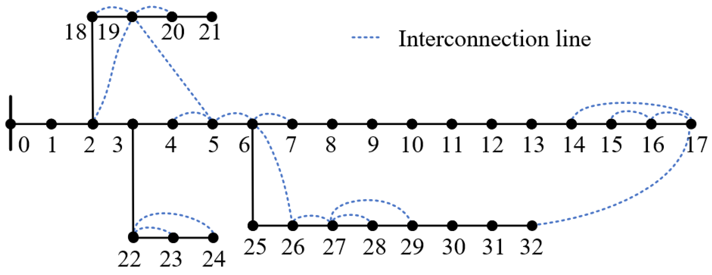
To evaluate the performance and robustness of the proposed two-stage robust optimization model under source–load uncertainty, a simulation test system is established based on the IEEE 33-bus distribution network. To enable robust planning of flexible interconnection under high DER penetration and to address potential issues such as transformer and line overloading, relatively large wind and PV capacities are incorporated in the system setup. Each bus is associated with a LVDA, and the system includes five wind (WD) turbines with a rated capacity of 0.5 MW each, and five photovoltaic (PV) units rated at 0.45 MW each. Taking into account practical engineering constraints such as physical distances between LVDAs and geographical wiring feasibility, a set of candidate interconnection lines with potential for deployment is identified. Figure 1 shows the configuration of wind and photovoltaic integration, as well as the candidate interconnection lines within the modified IEEE 33-bus distribution system.

For system operational constraints, the nodal voltage magnitude is bound between 0.95 p.u. and 1.05 p.u., with the voltage at the substation bus (Bus 0) fixed at 1.00 p.u. The maximum allowable loading rate for each LVDA transformer is set to 80%, and the minimum utilization ratio of DERs is enforced at 80%. Each LVDA is equipped with a VSC uniformly rated at 0.4 MW, and the maximum transmission capacity of each interconnection line is limited to 0.15 MW. All uncertainty-bound coefficients ${\lambda }_{\mathrm{wd}},{\lambda }_{\mathrm{pv}},{\lambda }_{\mathrm{dc}},{\lambda }_{\mathrm{ac}}$ are set to 5%. In terms of economic parameters, the daily investment cost of interconnection lines is set to $310/kilometer, with a project lifetime of 20 years and a discount rate of 5%. The daily cost for active power transmission is $15/MWh, and the load shedding penalty is likewise set to $600/MWh. All numerical simulations are carried out in the MATLAB R2020b environment on a personal computer equipped with a 2.50 GHz Intel i5 processor and 8 GB of RAM.

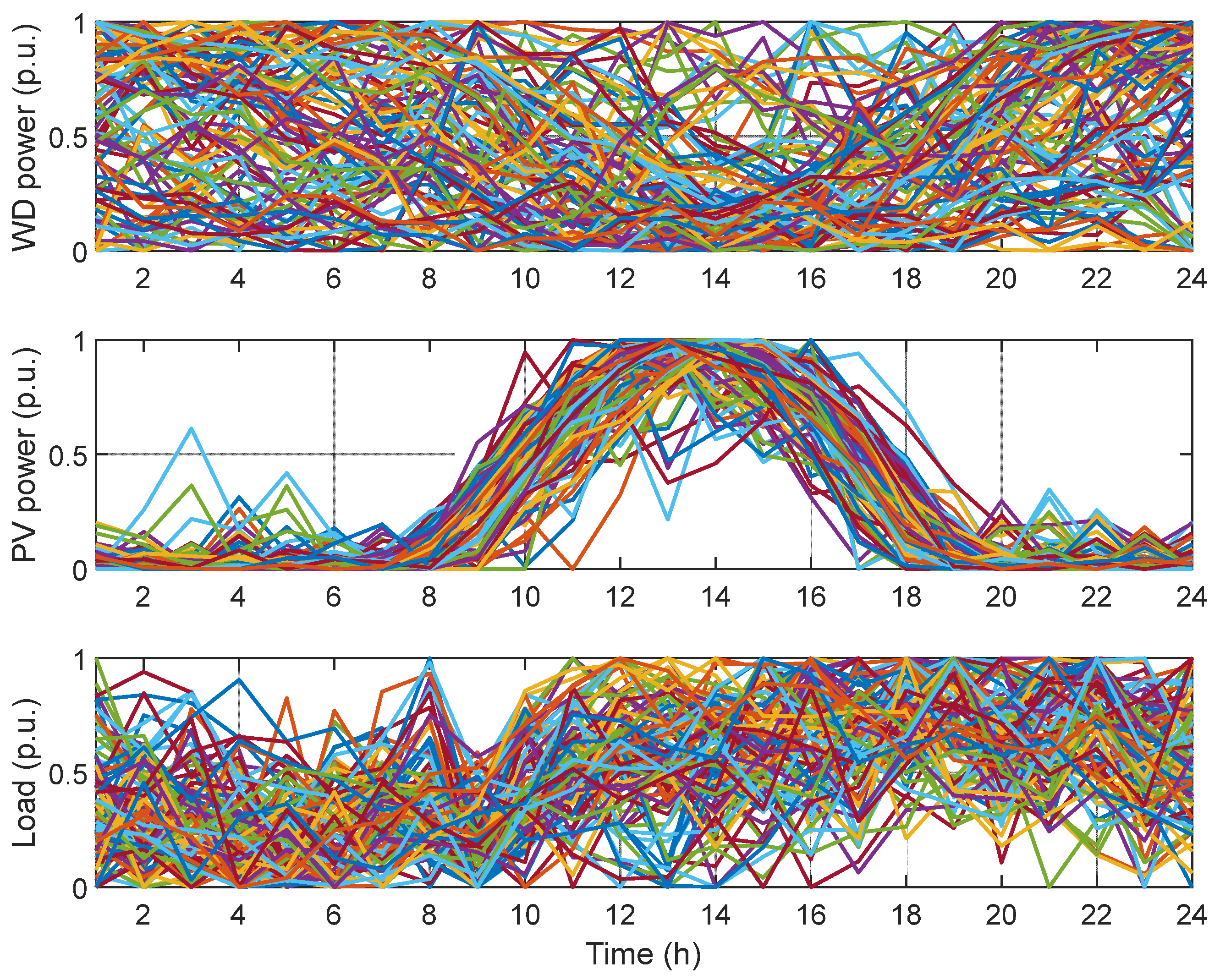
This work introduces a set of 1000 historical WD, PV, and load scenarios generated using a graphical model combined with Monte Carlo simulation [33,34]. Through a typical-day clustering approach, representative daily profiles were extracted to capture key temporal characteristics of these time-series data. Subsequently, stochastic perturbations were superimposed on these typical profiles to generate 100 diversified operational scenarios, thereby simulating a broad range of possible practical operating conditions. Figure 2 presents the normalized time-series profiles of wind power, solar PV generation, and aggregated load demand for these 100 scenarios. For simplicity and without loss of generality, AC and DC loads are assumed to follow the same normalized demand profile.

4.2. Performance Comparison

Figure 3 illustrates the convergence of the master–subproblem iteration using the CCG method with a distributed subproblem solver. The outer loop converges within three iterations, and each subproblem also converges in three iterations, as shown in the inset. The total solution time is only 39.1671 s, demonstrating that the proposed decomposition framework not only ensures rapid convergence but also achieves high computational efficiency in handling nonlinearity and uncertainty.

Figure 4 illustrates the planning results of flexible interconnection schemes among LVDAs obtained using the proposed robust optimization-based method. As observed, for several critical LVDAs integrating DERs (e.g., LVDAs 5, 10, 17, 19, and 24), the establishment of cross-LVDA interconnection lines forms energy-sharing corridors across geographically adjacent areas. These configurations not only enable localized utilization of renewable generation but also facilitate its effective accommodation on a broader, cross-regional scale, thereby enhancing the spatial flexibility of DER hosting capacity.

Although research on flexible interconnection planning in LVDNs has emerged only recently, most existing studies remain limited to evaluating transferred power volumes or verifying overload elimination in a few feeders under typical scenarios. By contrast, the following simulations demonstrate a more comprehensive assessment under deep uncertainty. The proposed robust planning framework inevitably sacrifices part of the economic optimality due to its conservative nature, but this trade-off enables substantial improvements in multiple aspects, including enhanced overload suppression, more stable voltage profiles, greater operational resilience, and strengthened autonomy across all LVDAs.

Under these synthesized scenarios, the proposed method is benchmarked against a conventional Stochastic Programming (SP) approach. Figure 5 depicts the maximum transformer loading rates for all 33 LVDAs over a full-day operation horizon. The results indicate that the SP method, constrained by its limited capacity to hedge against worst-case uncertainties, results in frequent overload conditions in specific LVDAs. These overloads significantly elevate the operational risk of DNs and reduce reliability margins. In contrast, the proposed method proactively coordinates inter-area load shifting and distributed energy balancing, alleviating critical bottlenecks and distributing stress more evenly, thereby improving overall operational resilience and security.

A more granular analysis is conducted for LVDAs 6 and 7, which are physically interconnected under both optimization strategies. Figure 6 illustrates the dynamic power flow along their interconnecting line, where positive values denote energy transfer from LVDA 6 to LVDA 7. The flow direction remains largely consistent throughout the operating period, indicating that LVDA 6 persistently exhibits higher load demand, while LVDA 7 provides buffer capacity to support power sharing. This coordinated interaction showcases the effectiveness of inter-LVDA energy exchange mechanisms in mitigating localized overloads and enhancing the flexibility and responsiveness of the overall system.

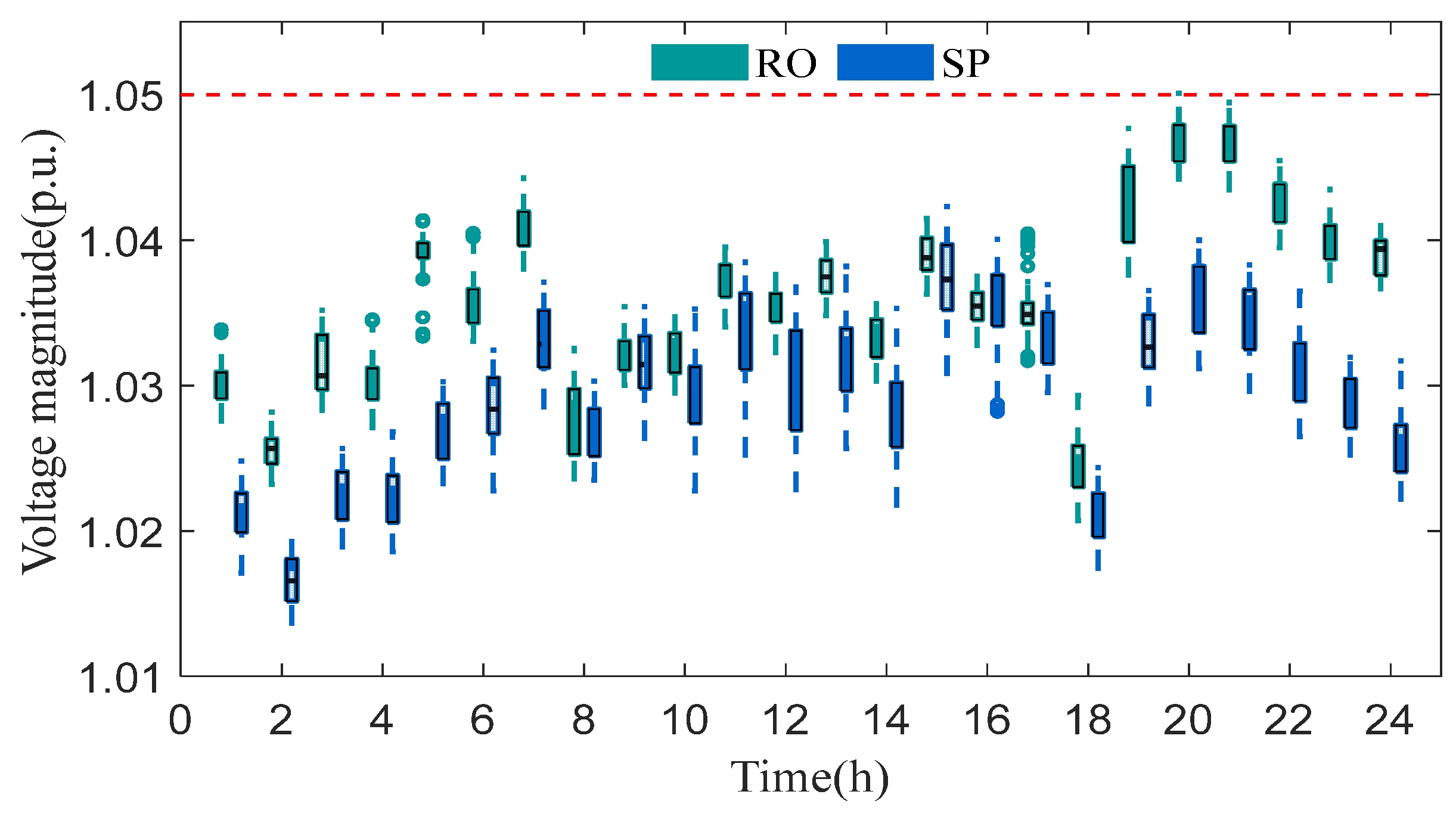
Figure 7 presents the voltage magnitude variation at a representative bus, namely bus 5, under both the SP and proposed methods. Both methods keep voltages within limits, but SP shows larger fluctuations, reflecting its vulnerability to uncertainty. Conversely, the proposed method suppresses deviations and maintains a steadier voltage profile throughout the time horizon. Although the voltage levels under the robust method are marginally elevated due to its inherent conservatism, this trade-off results in better voltage quality and improved system resilience against fluctuation-induced instability.

To further examine the autonomy-enhancing capabilities of the proposed method, Figure 8 and Figure 9 illustrate the active power output profiles of VSCs across all LVDAs. The absolute magnitude of VSC power serves as an indicator of internal energy balance: values closer to zero imply greater local generation–load matching and reduced reliance on inter-area power support. Compared with SP, the proposed approach reduces VSC power fluctuations, with exchanges often near zero, highlighting stronger LVDA self-sufficiency and reinforcing the decentralized operational autonomy of the DC distribution network.

Table 1. The expected daily apportioned overall cost.

	Investment Cost ($)	Operational Costs ($)	Total Costs ($)
RO	419.26	306.45	725.71
SP	337.84	313.73	651.57

summarizes the cost composition under both the proposed approach and the benchmark SP method. Despite the higher total cost incurred by the RO method, this economic premium is justified by significantly improved system-level performance under uncertainty. The increased cost primarily results from the conservative nature of RO, which explicitly accounts for a wide range of extreme disturbance scenarios. This leads to more proactive investment in flexibility resources and stronger operational safeguards, thereby ensuring system security even under worst-case conditions.

Table 2. Performance comparison under different ${\lambda }_{\mathrm{wd}}$ and ${\lambda }_{\mathrm{pv}}$ when ${\lambda }_{\mathrm{dc}}={\lambda }_{\mathrm{ac}}=5\%$.

${\mathit{\lambda }}_{\mathbf{wd}},{\mathit{\lambda }}_{\mathbf{pv}}$		2%	4%	6%	8%	10%
AI	RO	0.00046	0.00052	0.00073	0.0012	0.0019
	SP	0.0059	0.0063	0.0060	0.0077	0.0075
VQ	RO	0.0048	0.0051	0.0064	0.0074	0.0079
	SP	0.0078	0.0072	0.0084	0.0087	0.0093
OS	RO	0	0	0	0	0
	SP	25.374	26.526	28.902	28.981	27.442
DER utilization	RO	90.12%	89.46%	89.03%	86.62%	84.29%
	SP	90.69%	89.77%	89.34%	88.13%	88.26%

presents a comprehensive comparison of key performance indices under varying renewable penetration levels. To further quantify the differences observed in Figure 5, Figure 7, Figure 8 and Figure 9, three evaluation metrics are introduced as follows, namely the autonomy index (AI), the voltage quality index (VQ), and the overload severity index (OS), which, respectively, capture the self-sufficiency level of each LVDA, the voltage fluctuation amplitude under uncertainty, and the severity of overload events. These metrics allow for a systematic performance comparison between the RO and SP approaches under different maximum disturbance levels.

$$\mathrm{AI}={\displaystyle \frac{1}{N\times T}}{\displaystyle \sum _{t\in \mathcal{T}}{\displaystyle \sum _{i\in \mathcal{N}}{\left(p_{i,t}^{\mathrm{vsc}}\right)}^2}}$$

(28)

$$\mathrm{VQ}={\displaystyle \frac{1}{T}}{\displaystyle \sum _{t\in \mathcal{T}}\left(\max (U_t)-\min (U_t)\right)}$$

(29)

$$\mathrm{OS}={\displaystyle \frac{1}{N\times 100}}{\displaystyle \sum _{j=1}^{100}{\displaystyle \sum _{i\in \mathcal{N}}\max \left(\frac{p_{i,j,t}}{p_{i,j}^N}-{\beta }_{\max },0\right)}}$$

(30)

With increasing uncertainty, the RO approach consistently enhances local autonomy, suppresses voltage deviations, and mitigates overloading, demonstrating superior robustness. Regarding DER utilization, both methods maintain high average levels; however, the slightly higher utilization under SP is largely due to its limited scenario representation, which fails to capture rare yet extreme critical events. As a result, SP may suffer from severe curtailment or constraint violations under worst-case conditions. In contrast, the RO method maintains consistently high DER utilization across all realizations. Overall, the RO approach offers a more favorable trade-off between cost and reliability, making it a more practical and resilient solution for uncertainty-aware LVDC planning.

5. Conclusions

This study proposed a two-stage robust optimization framework for flexible interconnection planning in low-voltage distribution networks (LVDNs). Under distributed renewable energy uncertainty, the framework integrates investment decisions with worst-case operational scheduling. By employing a decomposition-based solution strategy, the original bi-level problem is reformulated into a tractable form, enabling fast and efficient computation. Based on simulation and comparative analysis, the following conclusions and outlook are drawn:

• In contrast to most existing studies that address only limited scenarios and local overload relief, the proposed robust planning delivers broader benefits, including reduced voltage fluctuations, elimination of severe overloads, stronger local self-sufficiency, and more reliable renewable integration. Although it incurs higher investment costs due to conservatism, these are offset by improvements in resilience and long-term reliability, making it well-suited for high-uncertainty environments.
• The evaluation is restricted to the IEEE 33-bus benchmark system, and broader validation on larger, real-world networks is still required; the robust formulation can be overly conservative compared with correlation-aware or probabilistic approaches.
• Future research should explore joint planning with other flexibility resources such as energy storage, soft open points, and demand response, as well as the adoption of distributionally robust or chance-constrained formulations to reduce conservatism while improving economic efficiency and scalability.

References

1. Fathabad, M.; Cheng, J.; Pan, K.; Qiu, F. Data-Driven Planning for Renewable Distributed Generation Integration. IEEE Trans. Power Syst. 2020, 35, 4357–4368. [Google Scholar] [CrossRef]
2. De Carne, G.; Buticchi, G.; Zou, Z.; Liserre, M. Reverse Power Flow Control in a ST-Fed Distribution Grid. IEEE Trans. Smart Grid 2018, 9, 3811–3819. [Google Scholar] [CrossRef]
3. Rehmani, M.H.; Reisslein, M.; Rachedi, A.; Erol-Kantarci, M.; Radenkovic, M. Integrating Renewable Energy Resources Into the Smart Grid: Recent Developments in Information and Communication Technologies. IEEE Trans. Ind. Inform. 2018, 14, 2814–2825. [Google Scholar] [CrossRef]
4. Ledva, G.S.; Balzano, L.; Mathieu, J.L. Real-Time Energy Disaggregation of a Distribution Feeder’s Demand Using Online Learning. IEEE Trans. Power Syst. 2018, 33, 4730–4740. [Google Scholar] [CrossRef]
5. Li, P.; Jin, B.; Wang, D.; Zhang, B. Distribution System Voltage Control Under Uncertainties Using Tractable Chance Constraints. IEEE Trans. Power Syst. 2019, 34, 5208–5216. [Google Scholar] [CrossRef]
6. Munikoti, S.; Abujubbeh, M.; Jhala, K.; Natarajan, B. An Information Theoretic Approach to Identify Dominant Voltage Influencers for Unbalanced Distribution Systems. IEEE Trans. Power Syst. 2022, 37, 4436–4446. [Google Scholar] [CrossRef]
7. Haider, Z.M.; Mehmood, K.K.; Khan, S.U.; Khan, M.O.; Wadood, A.; Rhee, S.-B. Optimal Management of a Distribution Feeder During Contingency and Overload Conditions by Harnessing the Flexibility of Smart Loads. IEEE Access 2021, 9, 40124–40139. [Google Scholar] [CrossRef]
8. Dharmapala, K.D.; Rajapakse, A.; Narendra, K.; Zhang, Y. Machine Learning Based Real-Time Monitoring of Long-Term Voltage Stability Using Voltage Stability Indices. IEEE Access 2020, 8, 222544–222555. [Google Scholar] [CrossRef]
9. Rabiee, A.; Keane, A.; Soroudi, A. Enhanced Transmission and Distribution Network Coordination to Host More Electric Vehicles and PV. IEEE Syst. J. 2022, 16, 2705–2716. [Google Scholar] [CrossRef]
10. Wang, J.; Zhou, N.; Chung, C.Y.; Wang, Q. Coordinated planning of converter-based dg units and soft open points incorporating active management in unbalanced distribution networks. IEEE Trans. Sustain. Energy 2020, 11, 2015–2027. [Google Scholar] [CrossRef]
11. Hakala, T.; Lähdeaho, T.; Järventausta, P. Low-voltage dc distribution—Utilization potential in a large distribution network company. IEEE Trans. Power Deliv. 2015, 30, 1694–1701. [Google Scholar] [CrossRef]
12. Gu, M.; Meegahapola, L.; Wong, K.L. Coordinated Voltage and Frequency Control in Hybrid AC/MT-HVDC Power Grids for Stability Improvement. IEEE Trans. Power Syst. 2021, 36, 635–647. [Google Scholar] [CrossRef]
13. Behera, P.K.; Pattnaik, M. Hybrid Energy Storage Integrated Wind Energy Fed DC Microgrid Power Distribution Control and Performance Assessment. IEEE Trans. Sustain. Energy 2024, 15, 1502–1514. [Google Scholar] [CrossRef]
14. Li, H.; Ren, Z.; Trivedi, A.; Verma, P.P.; Srinivasan, D.; Li, W. A noncooperative game-based approach for microgrid planning consider ing existing interconnected and clustered microgrids on an island. IEEE Trans. Sustain. Energy 2022, 13, 2064–2078. [Google Scholar] [CrossRef]
15. Lotfi, H.; Khodaei, A. AC versus DC microgrid planning. IEEE Trans. Smart Grid 2017, 8, 296–304. [Google Scholar] [CrossRef]
16. Liu, H.J.; Shi, W.; Zhu, H. Hybrid Voltage Control in Distribution Networks Under Limited Communication Rates. IEEE Trans. Smart Grid 2019, 10, 2416–2427. [Google Scholar] [CrossRef]
17. Watson, J.D.; Lestas, I. Frequency and Voltage Regulation in Hybrid AC/DC Networks. IEEE Trans. Control Syst. Technol. 2021, 29, 1839–1849. [Google Scholar] [CrossRef]
18. Peng, H.M.; Xiao, Q.H.; Tan, M.; Su, Y.X.; Li, H. Short-term maximum power supply capability assessment of low-voltage flexible interconnection distribution networks based on temporal convolutional neural network. South. Power Grid Technol. 2025, 1–11. [Google Scholar]
19. Niazi, Y.; Golshan, M.E.H.; Alhelou, H.H. Combined Firm and Renewable Distributed Generation and Reactive Power Planning. IEEE Access 2021, 9, 133735–133745. [Google Scholar] [CrossRef]
20. Sheng, H.; Wang, X. Applying Polynomial Chaos Expansion to Assess Probabilistic Available Delivery Capability for Distribution Networks with Renewables. IEEE Trans. Power Syst. 2018, 33, 6726–6735. [Google Scholar] [CrossRef]
21. Cao, F.; Zheng, J.Z.; Zheng, Y.X. Flexible Interconnection Planning Method for Distribution Substations in High-Quality Photovoltaic Resource Areas Based on VSC. South. Power Grid Technol. 2023, 17, 14–25. [Google Scholar] [CrossRef]
22. Cao, X.; Cao, T.; Gao, F.; Guan, X. Risk-Averse Storage Planning for Improving RES Hosting Capacity Under Uncertain Siting Choices. IEEE Trans. Sustain. Energy 2021, 12, 1984–1995. [Google Scholar] [CrossRef]
23. Poudyal, A.; Poudel, S.; Dubey, A. Risk-Based Active Distribution System Planning for Resilience Against Extreme Weather Events. IEEE Trans. Sustain. Energy 2023, 14, 1178–1192. [Google Scholar] [CrossRef]
24. Sheikhinejad, R.; Gharehpetian, G.B.; Rastegar, H. Active distribution network expansion planning considering microgrids for supplying critical loads. Sustain. Energy Grids Netw. 2024, 38, 101281. [Google Scholar] [CrossRef]
25. Li, C.; Li, Y.; Xia, S.; Wang, P. A two-stage adaptive-robust optimization model for active distribution network with high penetration wind power generation. IET Renew. Power Gener. 2023, 18, 1204–1217. [Google Scholar] [CrossRef]
26. Jing, H.; Zhao, C. A data expansion based piecewise regression strategy for incrementally monitoring the wind turbine with power curve. J. Cent. South Univ. 2023, 30, 1601–1617. [Google Scholar] [CrossRef]
27. Vilanova, A.; Kim, B.-Y.; Kim, C.K.; Kim, H.-G. Linear-Gompertz Model-Based Regression of Photovoltaic Power Generation by Satellite Imagery-Based Solar Irradiance. Energies 2020, 13, 781. [Google Scholar] [CrossRef]
28. Lee, G.-C. Regression-based methods for daily peak load forecasting in South Korea. Sustainability 2022, 14, 3984. [Google Scholar] [CrossRef]
29. Xiao, J.; Zu, G.; Zhou, H.; Zhang, X. Total quadrant security region for active distribution network with high penetration of distributed generation. J. Mod. Power Syst. Clean Energy 2021, 9, 128–137. [Google Scholar] [CrossRef]
30. Zhang, Z. An optimal scheduling of renewable energy in flexible interconnected distribution networks considering extreme scenarios. IET Renew. Power Gener. 2023, 17, 2531–2541. [Google Scholar] [CrossRef]
31. Li, J.; Xu, Z.; Zhao, J.; Zhang, C. Distributed online voltage control in active distribution networks considering PV curtailment. IEEE Trans. Ind. Inform. 2019, 15, 5519–5530. [Google Scholar] [CrossRef]
32. Sundarajoo, S.; Soomro, D.M. Optimal Load Shedding for Voltage Collapse Prevention Following Overloads in Distribution System. Int. J. Eng. 2023, 36, 1230–1238. [Google Scholar] [CrossRef]
33. Carmona, R.; Yang, X. Glasso model for electric load and wind power and monte Carlo scenario generation. arXiv 2021, arXiv:2111.14628. [Google Scholar] [CrossRef]
34. Available online: https://pan.baidu.com/s/1sTJSDBwQnZiHK8Yj0KdzbQ (accessed on 13 September 2025).
Figure 1. System configuration of the modified IEEE33-bus distribution system and candidate interconnection lines.
Electronics 14 03696 g001
Figure 2. The normalized time-series profiles of wind, PV, and load of 100 typical operational scenarios.
Electronics 14 03696 g002
Figure 3. The iterative convergence during the solution process of the RO model using the CCG and distributed algorithm.
Electronics 14 03696 g003
Figure 4. The flexible interconnection planning results for LVDAs obtained using the proposed method.
Electronics 14 03696 g004
Figure 5. The maximum transformer loading rates for all LVDAs under different methods.
Electronics 14 03696 g005
Figure 6. The dynamic power flows along the interconnecting line between LVDA 6 and 7.
Electronics 14 03696 g006
Figure 7. The voltage magnitude variation at bus 5 using RO and SP.
Electronics 14 03696 g007
Figure 8. The power transmission levels of VSCs across all LVDAs using RO.
Electronics 14 03696 g008
Figure 9. The power transmission levels of VSCs across all LVDAs using SP.
Electronics 14 03696 g009