Two-Dimensional Fractional Polar Volterra Series for Baseband Power Amplifier Behavioral Modeling

Abstract

This paper proposes a new behavioral model for radio-frequency power amplifiers (RF PAs) by extending the two-dimensional Polar Volterra series to fractional derivative order, using a numerical Mittag–Leffler-based formulation of fractional orthonormal generating functions. The motivation stems from the increasing need for accurate and computationally efficient models to represent nonlinearities and memory effects in wideband RF PAs, especially in energy-efficient 5G systems. The proposed method significantly reduces model complexity by lowering the number of estimated parameters while maintaining or improving modeling fidelity. To evaluate its performance, three different RF PA devices were used as test cases. The results demonstrated that the proposed approach achieved an over 81.5% reduction in the number of model parameters and improved modeling accuracy. Besides that, in a scenario with the same number of parameters, normalized mean square error (NMSE) gains of up to 8.72 dB were obtained. These findings support the method’s potential for practical use in RF PA behavioral modeling and digital predistortion applications.

1. Introduction

The design of radio-frequency power amplifiers (RF PAs) with wider bandwidths, higher linearity, and greater energy efficiency has garnered considerable attention due to the increasing demand for high data rates and low power consumption in fifth-generation (5G) wireless communication systems. In this context, energy-efficient RF PAs play a critical role in enabling system-level goals such as higher capacity, massive Multiple-Input Multiple-Output (MIMO), improved reliability, and overall cost-effectiveness [1]. Even in the 5G era, RF PAs remain the most cost-intensive and power-hungry components within radio transceivers. Their energy efficiency is significantly affected by the high peak-to-average power ratio (PAPR) introduced by Orthogonal Frequency-Division Multiplexing (OFDM) waveforms [2,3]. Moreover, the increased carrier frequencies and signal bandwidths—often in the hundreds of MHz—place additional demands on PA efficiency [4]. Since highly efficient RF PAs tend to be nonlinear, 5G signals with inherently high PAPR exacerbate the trade-off between linearity and efficiency [5].

A promising strategy to mitigate these effects is behavioral modeling using dynamic nonlinear models, such as Volterra series, which can be formulated in Cartesian (CV) or polar (PV) form. In such approaches, the PA output is modeled as a nonlinear polynomial function of the input, incorporating memory effects due to the dynamic nature of the system. The memory effects in RF PAs are modeled by delayed input dependencies and arise from various mechanisms, including faster effects such as non-flat frequency responses of the matching networks, as well as slower processes such as biasing circuitry, dynamic self-heating, trapping, and parasitic bipolar transistor effects [6], which are particularly relevant in low-cost implementations like small-cell base stations [7,8]. A widely adopted and cost-effective method to counteract PA nonlinearities is digital baseband predistortion (DPD), which applies a pre-compensating distortion to the input signal before amplification [9].

The design of a DPD unit based on the nonlinear and memory characteristics of the PA seeks to approximate the inverse of the PA’s transfer function [10]. While the Volterra-based models offer linear-in-the-parameters formulations suitable for least-squares (LS) optimization, their major drawback lies in the exponential growth of terms with increasing nonlinearity and memory depth. This results in substantial computational cost due to matrix inversions in LS estimation [11]. Several strategies have been proposed to reduce the number of parameters generated during the identification of RF PA models, without compromising accuracy or increasing computational complexity [12,13,14]. Among these, the Polar Volterra (PV) model originally proposed in [15,16] stands out. A more recent extension using Laguerre basis functions and independent truncations is presented in [17], further enhancing modeling flexibility.

More recently, fractional-order models have attracted increasing attention. Unlike classical integer-order formulations, fractional derivatives provide a more flexible mathematical framework for describing systems with memory, which makes them particularly effective for RF PA modeling. Linear fractional techniques have already been explored in several contexts, including Hammerstein systems [18], fractional-order neural networks [19,20,21], and fractional Volterra series [22,23,24]. In the broader 5G context, fractional modeling has also been successfully applied to channel identification and equalization in massive MIMO systems, demonstrating improved performance and reduced model complexity [25].

A key motivation for adopting fractional-order approaches in PA modeling lies in the fundamental differences between integer-order and fractional-order representations of memory. Integer-order (local) models approximate memory as a finite sum of exponentials associated with discrete-time constants. However, many PA memory mechanisms—such as bias-network dynamics, thermal self-heating, and charge trapping-exhibit long-range effects characterized by power-law decay and nearly constant phase over wide frequency spans. This type of “heavy-tailed” behavior is not well captured by a limited exponential basis. By contrast, fractional-order operators are intrinsically nonlocal and history-dependent, realizing memory through power-law kernels that naturally align with measured PA dynamics. As a result, fractional-order models often achieve more compact representations while maintaining, or even improving, modeling accuracy.

Motivated by these advances, this paper proposes a novel model that extends the two-dimensional polar Volterra formulation to the fractional derivative domain using a numerical Mittag-Leffler solution applied to a set of fractional orthonormal generating functions. The resulting model, referred to as the two-dimensional fractional polar Volterra ($2D\text{-}frPV$) model, is applied to the behavioral modeling of RF PAs and their inverse behavior.

The remainder of this paper is organized as follows: Section 2 presents the mathematical background of the Grünwald-Letnikov fractional derivative and the construction of the $2D\text{-}frPV$ model. Section 3 discusses the parameter extraction procedure for the proposed model. Section 4 provides experimental validation and performance evaluation results. Finally, a discussion of the modeling results and their implications is presented in Section 5.

2. Fractional Volterra Series

In this section, the fundamental concepts of fractional derivatives are first introduced in Section 2.1. Section 2.2 presents a simplified version of the Polar Volterra ($PV$) model, namely the two-dimensional PV ($2D\text{-}PV$), which retains only the one-dimensional and two-dimensional terms. Several simplified approaches to the Polar Volterra series have been proposed in the literature. Among these, the Memory Polynomial ($MP$) and the Generalized Memory Polynomial ($GMP$) models are the most prominent.

The $MP$ model considers only one-dimensional terms and employs a single complex input in each term, which is equivalent to fixing the phase polynomial truncation order to 1. The $GMP$ model, on the other hand, incorporates both one-dimensional and two-dimensional terms, while also restricting each term to a single complex input. In its original formulation, $GMP$ includes certain non-causal terms and multiple amplitude memory truncations. By removing the non-causal terms and adopting a single amplitude memory depth, $GMP$ can be regarded, similarly to $MP$, as a simplified version of the PV model, since it relies on only a subset of the terms generated by the full PV expansion.

The $2D$-$PV$ model can be viewed as an extension of the $GMP$, as well as of the model introduced in [14], by allowing the inclusion of multiple phase components through an increased phase polynomial truncation order. A common feature among all these models—$PV$, $MP$, $GMP$, and $2D\text{-}PV$—is their reliance on integer-order derivatives.

The main contribution of this work is the incorporation of fractional derivatives into this modeling framework, with the integer-order derivative being a particular case of the fractional one. Although the proposed approach could be applied starting from $MP$, $GMP$, or even the full PV model, the $2D$-$PV$ was selected as the baseline due to its balance between model complexity and representational capability. Accordingly, Section 2.3 details the central contribution of this paper: the incorporation of fractional derivatives into a reduced-order $PV$ model, namely the $2D$-$PV$.

2.1. Basic Notions of Grünwald-Letnikov Fractional Derivative

The arbitrary order or non-integer-order derivative function can be represented with the symbol ${}_{a}D_t^{\alpha }$, where $\alpha$ is the fractional derivative order, D is a derivative operator, a and t represent, respectively, the lower and upper bounds of the fractional differentiation operator D. In the literature, there are several definitions of fractional derivatives: the Riemann-Liouville definition, the Caputo definition, and the Grünwald-Letnikov definition [26]. The Grünwald-Letnikov definition of the fractional derivative was used in this work for the development of Fractional Volterra model since it is suggested for obtaining numerical solutions in practical applications of fractional-order systems using numerical methods [27].

The Grünwald-Letnikov Fractional Derivative ${}_{a}D_t^{\alpha }$ or simply $D^{\alpha }$ of a continuous-time function $f\left(t\right)$ [26], is given by:

$$D^{\alpha }f\left(t\right)=\underset{h\to 0}{lim}\sum _{j=0}^{\left|{\displaystyle \frac{t-a}{h}}\right|}{(-1)}^j\left({\displaystyle \genfrac{}{}{0pt}{}{\alpha }{j}}\right)f(t-jh),$$

(1)

where $\left({\displaystyle \genfrac{}{}{0pt}{}{\alpha }{j}}\right)={\displaystyle \frac{\Gamma (\alpha +1)}{\Gamma (j-1)\Gamma (\alpha -j+1)}}$ is the usual notation for the binomial coefficients. A simple formulation of the Grünwald–Letnikov derivative in the discrete-time fractional derivative order [28], is described by the equation:

$$D^{\alpha }{f}_{\tau }=f_{\tau }+\sum _{j=0}^{\tau }{\Phi }_{\tau }\left({\alpha }_{\tau }\right)f_{\tau -j},\tau =0,1,\cdots$$

(2)

where $\alpha \in [0,2]$ is the fractional order and

$$\begin{array}{cc}\hfill {\Phi }_{\tau }& =diag\left[\begin{array}{cccc}{\Phi }_1\left({\alpha }_1\right)& {\Phi }_2\left({\alpha }_2\right)& \cdots & {\Phi }_{\tau }\left({\alpha }_{\tau }\right)\end{array}\right],\hfill \end{array}$$

(3)

$$\begin{array}{cc}\hfill {\Phi }_{\tau }\left({\alpha }_{\tau }\right)& ={(-1)}^{\tau }\left\{\begin{array}{cc}1,\hfill & \mathrm{if}\tau =0\hfill \\ {\displaystyle \frac{\alpha (\alpha -1)\cdots (\alpha -\tau +1)}{\tau !}},\hfill & \mathrm{if}\tau =1,2,3,\dots \hfill \end{array}\right..\hfill \end{array}$$

(4)

The Laplace transform of the Grünwald–Letnikov fractional operator [29] under zero-initial conditions is given by:

$$\mathcal{L}\left[D^{\alpha }f\left(t\right)\right]=s^{\alpha }F\left(s\right),$$

(5)

2.2. Two-Dimensional Polar Volterra Series

The discrete-time Polar Volterra series ($PV$) [15] is given by:

$$\begin{array}{cc}\hfill \tilde{y}\left(n\right)& =\sum _{p_1=1}^{P_1}\sum _{p_2=1}^{P_2}\sum _{m_1=0}^M\cdots \sum _{m_{p_1}=m_{p_1-1}}^M\sum _{l_1=0}^L\cdots \sum _{l_{p_2}=l_{p_2}-1}^L\sum _{l_{p_2+1}=0}^L\cdots \sum _{l_{2p_2-1}=l_{2p_2-2}}^L\hfill \\ & {\tilde{h}}_{p_1,2p_2-1}(m_1,\cdots ,m_{p_1},l_1,\cdots ,l_{2p_2-1})\prod _{q=1}^{p_1}a(n-m_q)\prod _{r=1}^{p_2}{e}^{j\varphi (n-l_r)}\prod _{s=p_2+1}^{2p_2-1}{e}^{-j\varphi (n-l_s)},\hfill \end{array}$$

(6)

where $\tilde{h}(·)$ are complex coefficients, $a\left(n\right)$ and ${\varphi }_n$ represent, respectively, the amplitude and phase components of the input complex-valued envelope signal $\tilde{x}\left(n\right)$, $P_1$ is the amplitude polynomial truncation order, M is the amplitude memory duration, $P_2$ is the phase polynomial truncation order and L is the phase memory duration.

The number of generated coefficients in the $PV$ model of Equation (6) is strongly conditioned by the four truncation factors $P_1$, M, $P_2$ and L. However, the number of coefficients increases very rapidly with increasing values of these truncation factors $P_1$, $P_2$, M, and L. An increase in RF PA coefficients has a direct effect on increasing the computational complexity of a Polar Volterra model, which does not allow for a compromise between the accuracy and the computational effort. On the other hand, regardless of the values of the polynomial and memory truncation factors, greater accuracy in the $PV$ model means a higher amount of generated parameters. The consequence of this is that it becomes a challenge to achieve an RF PA operating at its highest energy efficiency. However, a hardware DPD implementation based on the RF PA characteristic will have a high energy consumption that can be even higher depending on the number of multiplications among $a\left(n\right)$ and $a(n-m_q)$ where $m_q\in [0,M]$, $e^{j\varphi \left(n\right)}$ and $e^{j\varphi (n-l_r)}$ where $l_r\in [0,L]$, $e^{j\varphi \left(n\right)}$ and $e^{-j\varphi (n-l_s)}$ where $l_s\in [0,L]$, products of the amplitudes, products of the positive phases and products of the negative phases, all required in the $PV$ model. Therefore, this makes the power consumption of the RF PA and DPD acting together greater than the power consumption of the RF PA acting alone. Some researchers have proposed strategies to reduce the number of generated parameters in the $PV$ model of Equation (6) without, however, reducing its accuracy in any way and without compromising the computational effort performed in the low-pass equivalent behavioral modeling of an RF PA [12,13,14]. Some of these strategies include simplifying the $PV$ model to decrease the influence of past time instants. This simplification technique of the Volterra series with polar terms considers only one-dimensional and two-dimensional terms. Thus, considering only the one-dimensional and two-dimensional terms as in [14], Equation (6) can be rewritten, in general, as the two-dimensional Polar Volterra model, ($2D\text{-}PV$):

$$\begin{array}{cc}\hfill {\tilde{y}}_{2D-PV}\left(n\right)=& \sum _{p_1=1}^{P_1}\sum _{p_2=0}^{p_1-1}\sum _{m_1=0}^M\sum _{m_2=m_1+1}^M\sum _{p_3=1}^{P_3}\sum _{p_4=0}^{p_3-1}\sum _{l_1=0}^L\sum _{l_2=l_1+1}^L\sum _{p_5=1}^{p_3-1}\sum _{p_6=0}^{p_5-1}\sum _{l_3=0}^L\sum _{l_4=l_3+1}^L\hfill \\ & {\tilde{h}}_{p_1,p_2,p_3,p_4}(m_1,m_2,l_1,l_2,l_3,l_4)a^{(p_1-p_2)}\left(n-m_1\right)\times a^{p_2}\left(n-m_2\right)\times \hfill \\ & {\left(e^{j\varphi \left(n-l_1\right)}\right)}^{(p_3-p_4)}\times {\left(e^{j\varphi \left(n-l_2\right)}\right)}^{p_4}\times {\left(e^{-j\varphi \left(n-l_3\right)}\right)}^{(p_5-p_6)}\times {\left(e^{-j\varphi \left(n-l_4\right)}\right)}^{p_6},\hfill \end{array}$$

(7)

where $P_1$ is the amplitude polynomial truncation order, M is the amplitude memory duration, $P_3$ is the phase polynomial truncation order and L is the phase memory duration. In this $2D\text{-}PV$ model, the one-dimensional terms are related to the contributions of the amplitude and phase input signals at a single time sample, where the products are performed when the amplitude and phase memory delays are $m_q=l_r=l_s$, independently of the amplitude and phase polynomial truncation orders. two-dimensional terms are related to the contributions of the amplitude and phase input signals at two different time samples, consecutive or not, if the products are performed through two distinct memory delays. Three-dimensional terms are neglected, as well as terms that are related to the amplitude and phase input signals at more than three time samples.

2.3. Two-Dimensional Fractional Polar Volterra Series

Assuming two-dimensional Polar Volterra kernels, ${\tilde{h}}_{p_1,p_2,p_3,p_4}(·)$, represent a model containing the maximum order of the nonlinearity, the full length of amplitude memory $\left[0;M\right]$, all of the phase memory length $\left[0;L\right]$ and, without taking into account the type, characteristics and amount of measured samples of the input and the output signals, the accuracy of the $2D\text{-}PV$ model can be significantly improved without, however, increasing in any way the amount of generated coefficients in the model. This increase in accuracy can be achieved depending on how the instantaneous and previous samples of the amplitude and phase signals are, simultaneously or separately, mathematically manipulated. One of these tools available in the literature is the linear fractional differentiation models [22], which have proven to be efficient in identifying systems. Considering that the $2D\text{-}PV$ model in Equation (2) can be seen as a generalization of linear models based on the two-dimensional Polar Volterra series, this mean that the $2D\text{-}PV$ model can be expanded to the fractional derivatives domain as a linear fractional differentiation model in which the kernels ${\tilde{h}}_{p_1,p_2,p_3,p_4}(m_1,m_2,l_1,l_2,l_3,l_4)$ can be extended to fractional orthonormal bases Volterra kernels [30], ${\tilde{c}}_{p_1,p_2,p_3,p_4}({\tau }_1,{\tau }_2,{\sigma }_1,{\sigma }_2,{\sigma }_3,{\sigma }_4)$, using a set of fractional orthonormal generating functions, where their representation in discrete-time domain numerically corresponds to the Grünwald–Letnikov fractional derivative, since the Grünwald–Letnikov definition is best suited to describe fractional-order calculus problems with zero-initial conditions [31]. By applying the Gram–Schmidt orthogonalization procedure on a set of generating functions, refs. [32,33] extended orthonormal basis functions to a fractional derivative order for systems approximation. The result of this extension is the so-called fractional orthonormal generating functions, in which their general representation is defined through the Laplace transform is given by:

$$F_{\tau }\left(s\right)={\displaystyle \frac{1}{{(s^{{\alpha }_{\tau }}+{\beta }_{\tau })}^{\tau }}},\tau =1,2,3,\cdots ,$$

(8)

where ${\alpha }_{\tau }$ is the fractional order and ${\beta }_{\tau }$ is a parameter belonging to the set of strictly positive real numbers and will be defined as ${\beta }_{\tau }=1$ later. These two parameters, $\beta$ and $\alpha$, represent the conditions stem arising from the stability theorem which defines that a commensurate system of order $0<\alpha <1$ or $1<\alpha <2$ described by a transfer function $F\left(s\right)$, Equation (8), is stable if and only if $\left|arg\left(\beta \right)\right|>\alpha {\displaystyle \frac{\pi }{2}}$ [34] or $\left|arg\left(s^{\alpha }\right)\right|<\alpha {\displaystyle \frac{\pi }{2}}$ [31].

Due to their similarity to the integer-order state-space models representation [35], fractional-order models can also be represented in state-space form. Thus, the expansion dynamics of the two-dimensional Polar Volterra model into the fractional derivatives domain can be achieved using the fractional-order state-space modeling given by:

$$\begin{array}{cc}\hfill D^{\alpha }f\left(t\right)& =Af\left(t\right)+Bu\left(t\right),\hfill \end{array}$$

(9)

$$\begin{array}{cc}\hfill y\left(t\right)& =Cf\left(t\right)+Du\left(t\right),\hfill \end{array}$$

(10)

where $u\left(t\right)$ and $y\left(t\right)$ are, respectively, the $m\times 1$ input and the $p\times 1$ output vectors. A is the $n\times n$ matrix and it describes the dynamics of the fractional derivative system, B is the $n\times 1$ input vector and it describes the linear transformation by which the input signal $u\left(t\right)$ influences the next state, C is the $p\times p$ output matrix, and it describes how the state is transferred to the output, D is the $p\times 1$ feed-forward vector, $\alpha$ is the commensurate fractional-order and $D^{\alpha }$ is the Grünwald–Letnikov fractional derivative [29] of order $\alpha$. $f\left(t\right)$ is the $t\times 1$ fractional generating function state-space vector in the continuous-time domain. However, the Laplace transform of the fractional generating function $F\left(s\right)$ in the continuous-time domain $f\left(t\right)$ of order $s^{\alpha }$ is not analytically derivable, but its series expansion can be obtained [27]. In this way, expanding $F\left(s\right)$ of Equation (8) as a series expansion yields that:

$$F\left(s\right)={\displaystyle \frac{1}{s^{\alpha }+\beta }}={\displaystyle \frac{1}{s^{\alpha }}}\sum _{\gamma =0}^{\infty }{\displaystyle \frac{{(-\beta )}^{\gamma }}{s^{\alpha }}}.$$

(11)

This means that the impulse response $f\left(t\right)$ can be determined through the Laplace transform of the fractional orthonormal generating function $F\left(s\right)$ expanded in a series, resulting in a numerical Mittag–Leffler function:

$$f\left(t\right)={\mathcal{L}}^{-1}\left\{{\displaystyle \frac{1}{s^{\alpha }}}\sum _{\gamma =0}^{\infty }{\displaystyle \frac{{(-\beta )}^{\gamma }}{s^{\alpha }}}\right\}=t^{\alpha -1}\sum _{\gamma =0}^{\infty }{\displaystyle \frac{{(-\beta )}^{\gamma }{t}^{\alpha \gamma }}{\Gamma (\alpha \gamma +\alpha )}}.$$

(12)

Using the definition of the Laplace transform of Grünwald–Letnikov fractional operator in Equation (4) including its existence condition at $t=0$, considering that $D^{\alpha }f\left(t\right)=0$ since $f\left(t\right)=0,\forall t<0$ [36], it leads to define the fractional orthonormal generating function in Equation (12), which forms a basis in $L_2\left(\right[0,\infty \left[\right)$ [33], at $t=0^{+}$ as:

$$f_{\tau }\left(t\right)=t^{{\alpha }_{\tau }-1}\sum _{\gamma =0}^{\infty }{\left.\begin{array}{c}{\displaystyle \frac{{(-{\beta }_{\tau })}^{\gamma }{t}^{{\alpha }_{\tau }\gamma }}{\Gamma ({\alpha }_{\tau }\gamma +{\alpha }_{\tau })}}\end{array}\right|}_{t=0^{+}},\tau =1,2,3,\cdots .$$

(13)

To facilitate understanding of the fractional expansion process using a set of fractional generating functions in Equation (11), let us consider the third order of the Volterra series with Cartesian coordinates:

$$\tilde{y}\left(t\right)={\tilde{y}}_1\left(t\right)+{\tilde{y}}_3\left(t\right),$$

(14)

where

$$\begin{array}{c}\hfill {\tilde{y}}_1\left(t\right)=\sum _{q_1=0}^M{\tilde{h}}_{1,q_1}\tilde{x}(t-m_{q_1}),\end{array}$$

(15)

$$\begin{array}{c}\hfill {\tilde{y}}_3\left(t\right)=\sum _{q_1=0}^M\sum _{q_2=q_1}^M\sum _{q_3=0}^M{\tilde{h}}_{3,(q_1,q_2,q_3)}\tilde{x}(t-m_{q_1})\tilde{x}(t-m_{q_2}){\tilde{x}}^{\ast }(t-m_{q_3}).\end{array}$$

(16)

Assuming that the amount of fractional generating functions K corresponds to the memory length M of (15) and (16), therefore, the coefficients ${\tilde{h}}_{1,q_1}$ and ${\tilde{h}}_{3,(q_1,q_2,q_3)}$ can be expanded through a set of K fractional generating functions [22] by:

$$\begin{array}{c}\hfill {\tilde{h}}_{1,q_1}\approx \sum _{{\tau }_1=1}^{K+1}{\tilde{c}}_{1,{\tau }_1}{f}_{{\tau }_1}\left(t\right),\end{array}$$

(17)

$$\begin{array}{c}\hfill {\tilde{h}}_3(q_1,q_2,q_3)\approx \sum _{{\tau }_1=1}^{K+1}\cdots \sum _{{\tau }_3=1}^{K+1}{\tilde{c}}_{3,({\tau }_1,{\tau }_2,{\tau }_3)}{f}_{{\tau }_1,{\tau }_2,{\tau }_3}\left(t\right).\end{array}$$

(18)

Similarly, both components (15) and (16) can be expanded by fractional generating functions in the continuous-time domain as:

$$\begin{array}{c}\hfill {\tilde{y}}_1\left(t\right)=\sum _{{\tau }_1=1}^{K+1}{\tilde{c}}_{1,{\tau }_1}{\mathcal{L}}^{-1}\left[F_{{\tau }_1}\left(s\right)\tilde{X}\left(s\right)\right],\end{array}$$

(19)

$$\begin{array}{c}\hfill {\tilde{y}}_3\left(t\right)=\sum _{{\tau }_1=1}^{K+1}\sum _{{\tau }_2={\tau }_1}^{K+1}\sum _{{\tau }_3=1}^{K+1}{\tilde{c}}_{3,({\tau }_1,{\tau }_2,{\tau }_3)}{\mathcal{L}}^{-1}\left[F_{{\tau }_1}\left(s\right)\tilde{X}\left(s\right)\right]{\mathcal{L}}^{-1}\left[F_{{\tau }_2}\left(s\right)\tilde{X}\left(s\right)\right]{\mathcal{L}}^{-1}\left[F_{{\tau }_3}\left(s\right){\tilde{X}}^{\ast }\left(s\right)\right],\end{array}$$

(20)

where $F_{\tau }\left(s\right)$ and $\tilde{X}\left(s\right)$ are, respectively, the fractional orthonormal generating functions and the input complex-valued envelope signal, both in the frequency domain.

If ${\tilde{J}}_{\tau }\left(t\right)={\mathcal{L}}^{-1}\left[F_{\tau }\left(s\right)\tilde{X}\left(s\right)\right]$ then, calculating ${\mathcal{L}}^{-1}\left[F_{\tau }\left(s\right)\tilde{X}\left(s\right)\right]$ results in a convolution product of $f_{\tau }\left(t\right)$ and $\tilde{x}\left(t\right)$ expressed by:

$${\tilde{J}}_{\tau }\left(t\right)=f_{\tau }\left(t\right)\otimes \tilde{x}\left(t\right)=t^{{\alpha }_{\tau }-1}\sum _{\gamma =0}^{\infty }{\left.\begin{array}{c}{\displaystyle \frac{{(-{\beta }_{\tau })}^{\gamma }{\left(nT\right)}^{{\alpha }_{\tau }\gamma }}{\Gamma ({\alpha }_{\tau }\gamma +{\alpha }_{\tau })}}\end{array}\right|}_{t=0^{+}}\otimes \tilde{x}\left(t\right).$$

(21)

However, this Equation (21) can be rewritten in the discrete-time domain assuming that $t=nT$:

$${\tilde{J}}_{\tau }\left(nT\right)={\left(nT\right)}^{{\alpha }_{\tau }-1}\sum _{\gamma =0}^{\infty }{\left.\begin{array}{c}{\displaystyle \frac{{(-{\beta }_{\tau })}^{\gamma }{\left(nT\right)}^{{\alpha }_{\tau }\gamma }}{\Gamma ({\alpha }_{\tau }\gamma +{\alpha }_{\tau })}}\end{array}\right|}_{nT=0^{+}}\otimes \tilde{x}\left(n\right),$$

(22)

where T is the sampling period of the input complex-valued envelope signal $\tilde{x}\left(n\right)$. The input signal $\tilde{x}\left(n\right)$ can be represented by its amplitude and phase components, $a\left(n\right)$ and $e^{j{\varphi }_n}$, respectively. Substituting both components in Equation (22) results in:

$${\tilde{J}}_{\tau }\left(nT\right)={\lambda }_{\tau }\left(n\right)·e^{j{\varphi }_n}.$$

(23)

The flexibility of the magnitude ${\lambda }_{\tau }\left(n\right)$ is provided by the shift operator z over amplitude $a\left(n\right)$, such that $za\left(n\right)=a(n+1)$. Therefore, the two-dimensional Polar Volterra model ($2D\text{-}PV$) presented in (7) can be extended to a fractional derivative order through a set of fractional orthonormal generating functions in the discrete-time domain, resulting in the two-dimensional fractional Polar Volterra model ($2D\text{-}frPV$), expressed through the state-space realization:

$$\begin{array}{c}\hfill {\lambda }_{\tau }(n+1)={\Phi }_{\tau }{\Psi }_{\tau }{\lambda }_{\tau }\left(n\right)+B_{\tau }a(n+1),\end{array}$$

(24)

$$\begin{array}{c}\hfill {\tilde{y}}_{2D-frPV}\left(n\right)=\mathcal{H}\left({\tilde{J}}_1\left(n\right),{\tilde{J}}_2\left(n\right),\cdots ,{\tilde{J}}_{\tau }\left(n\right)\right),\end{array}$$

(25)

where ${\lambda }_0\left(n\right)$ represents the zero-initial condition of the magnitude ${\lambda }_{\tau }\left(n\right)$, the parameter ${\Phi }_{\tau }$ is defined in Equations (3) and (4), $B_{\tau }=\left[ones(\tau ,1)\right],\tau =1,2,3,\cdots$ and

$$\begin{array}{c}\hfill {\Psi }_{\tau }=diag\left[\begin{array}{c}{f}_1\left(n\right),f_2\left(n\right)f_1\left(n\right),\cdots ,{\left(f_{\tau }\left(n\right)\right)}^{\tau }\end{array}\right],\end{array}$$

(26)

$$\begin{array}{c}\hfill f_{\tau }\left(n\right)={\left(nT\right)}^{{\alpha }_{\tau }-1}\sum _{\gamma =0}^{\infty }{\left.{\displaystyle \frac{{(-{\beta }_{\tau })}^{\gamma }{\left(nT\right)}^{{\alpha }_{\tau }\gamma }}{\Gamma ({\alpha }_{\tau }\gamma +{\alpha }_{\tau })}}\right|}_{nT=0^{+}}.\end{array}$$

(27)

Analytically, the two-dimensional fractional Polar Volterra model ($2D\text{-}frPV$) can be given by:

$$\begin{array}{cc}\hfill {\tilde{y}}_{2D-frPV}\left(n\right)& =\sum _{p_1=1}^{P_1}\sum _{p_2=0}^{p_1-1}\sum _{{\tau }_1=0}^K\sum _{{\tau }_2={\tau }_1+1}^K\sum _{p_3=1}^{P_3}\sum _{p_4=0}^{p_3-1}\sum _{{\sigma }_1=0}^Q\sum _{{\sigma }_2={\sigma }_1+1}^Q\sum _{p_5=1}^{p_3-1}\sum _{p_6=0}^{p_5-1}\sum _{{\sigma }_3=0}^Q\sum _{{\sigma }_4={\sigma }_3+1}^Q\hfill \\ & {\tilde{c}}_{p_1,p_2,p_3,p_4}({\tau }_1,{\tau }_2,{\sigma }_1,{\sigma }_2,{\sigma }_3,{\sigma }_4){\lambda }_{{\tau }_1}^{(p_1-p_2)}\left(n\right)\times {\lambda }_{{\tau }_2}^{p_2}\left(n\right)\times {\left(e^{j\varphi \left(n-{\sigma }_1\right)}\right)}^{(p_3-p_4)}\times \hfill \\ & {\left(e^{j\varphi \left(n-{\sigma }_2\right)}\right)}^{p_4}\times {\left(e^{-j\varphi \left(n-{\sigma }_3\right)}\right)}^{(p_5-p_6)}\times {\left(e^{-j\varphi \left(n-{\sigma }_4\right)}\right)}^{p_6}.\hfill \end{array}$$

(28)

where $P_1$ is the amplitude polynomial truncation order, K is the amplitude memory duration, $P_3$ is the phase polynomial truncation order and Q is the phase memory duration. As in the $2D\text{-}PV$ model, in this new $2D\text{-}frPV$ approach, the one-dimensional terms are related to the contributions of the amplitude and phase input signals at a single time sample, where the products are performed when the amplitude and phase memory delays are $m_q=l_r=l_s$. This part of the model, regardless of the amplitude and phase polynomial truncation orders, maps memory effects in a simple way, reducing the multidimensional kernels to one-dimensional contributions. In the two-dimensional terms, the contributions of the amplitude and phase input signals are related in two different time samples, whether consecutive or not, if the products are performed using two distinct memory delays, and this maps the memory effect in a dual manner, reducing multidimensional kernels to the two-dimensional contributions. Three-dimensional terms and terms that are related to the amplitude and phase input signals at more than three time samples are neglected.

Unlike the memory polynomial [12], memory polynomial of one- and two-dimensional terms and generalized memory polynomial [13], where these three models widely used in the literature represent particular cases of the $2D\text{-}PV$ model, in the proposed $2D\text{-}frPV$ model, there is polynomial truncation for the evolution of the phase samples, which forces certain phase samples to be of the same time instant and other phase samples to be at different time instants from the amplitude samples. In the highly efficient wideband and very high linear low-pass equivalent models where the input excitation is an amplitude and phase modulated envelope signal, the recognition of the RF PA and DPD nonlinear distortions cannot be completely determined by the static and dynamic amplitude-to-amplitude intermodulation (AM-AM) distortion, but accurate amplitude modulation to phase modulation distortion (AM-PM) that arises in the physical characteristics of transistors (gate-source, gate-drain and drain-source capacitances) is also required [37] or when the nonlinear circuits has large memory effects and the input signal consisting of one or many components with one, two, or three tones [38], can model all memory effects using amplitude and phase samples at a maximum of two different time instants. This proposed $2D\text{-}frPV$ model can also evaluate the nonlinearities of RF PA by measuring AM-AM and AM-PM curves at the frequencies of interest.

The amount of generated parameters by the $2D\text{-}PV$ and $2D\text{-}frPV$ models is based on the multiplication of the input signal up to a maximum of two time instants. These two models can model envelope signal phase variation phenomena, they can manipulate mechanisms such as phase modulation to amplitude modulation (PM-AM) conversion, which indicates changes in the output amplitude envelope as a function of the input phase envelope variation, and mechanisms such as phase modulation to phase modulation conversion (PM-PM), which indicates changes in the difference between the output and input phases as a function of the input phase envelope variation [39]. They are also able to model nonlinear and linear memory effects of the 5G signal based on past amplitude and phase samples.

3. Modeling Extraction

The $2D\text{-}frPV$ model proposed in (28) uses the RF PA extraction method with constraint in a single free parameter, namely fractional order $\alpha$, which should be considered based on prior knowledge of the model under study. In a practical scenario, the selection of the fractional order $\alpha$ can be done in the same way as the expansion of Fourier functions, where the first term of the approximation of a fractional transfer function by the fractional orthonormal base order is the dominant term; however, using this procedure to find the fractional order $\alpha$ requires the use of a logarithmic slope plot [40] associated with the system impulse response. Assuming that there is a priori knowledge about the $\alpha$ for all distortions and orders of nonlinearity of the low-pass equivalent RF PA model, choosing the $\alpha$ can involve optimizing an objective function which minimizes the approximation error between the estimated and desired data so that the resulting fractional order $\alpha$ is close to the fundamental fractional order $\widehat{\alpha }$, which models all distortions and nonlinearities of the low-pass equivalent RF PA model. It is an objective function which depends entirely on the fractional-order dynamic $\alpha$ and whose resolution allows for a fast convergence of the $2D\text{-}frPV$ model. The objective function ($OF$) is defined as:

$$OF(n,\alpha )=\sum _{n=1}^N{\left|\tilde{y}\left(n\right)-\tilde{\psi }{(n,\alpha )}^T\Theta \left(\alpha \right)\right|}^2,$$

(29)

where the vector $\tilde{\psi }(n,\alpha )$ contains all multiplications between ${\lambda }_{\tau }\left(n\right)$ and $e^{j{\varphi }_n}$ of Equation (28). The matrix $X(n,\alpha )$ is made up of all vectors $\tilde{\psi }(n,\alpha )$); therefore, the vector $\Theta \left(\alpha \right)$ containing the coefficient ${\tilde{c}}_{p_1,p_2,p_3,p_4}(·)$ of the $2D\text{-}frPV$ model can be estimated by the least-squares method inside a nonlinear optimization with a constrain on the fractional-order values at $0<\alpha <1$ or $1<\alpha <2$, through:

$$\Theta \left(\alpha \right)={\left(X{(n,\alpha )}^{H}X(n,\alpha )\right)}^{-1}X{(n,\alpha )}^{H}Y\left(n\right);$$

(30)

in which the minimum argument that finds the local minimum and returns the dominant fraction $\widehat{\alpha }$ is given by:

$$\left(\widehat{\alpha }\right)=\underset{\alpha }{argmin}OF(n,\alpha ).$$

(31)

4. Results

Three different devices under test (DUTs) are investigated. In each of the DUTs, a set of estimation and validation input and output samples was used for identification and validation of the proposed $2D\text{-}frPV$ model and of the $PV$ and $2D\text{-}PV$ models. Their modeling results of the direct and inverse RF PA transfer characteristic were analyzed. For the three DUTs, the set of fractional orthonormal generator functions in the discrete-time domain defined in Equation (27) was conditioned on $n=1$ and $T=0.26$.

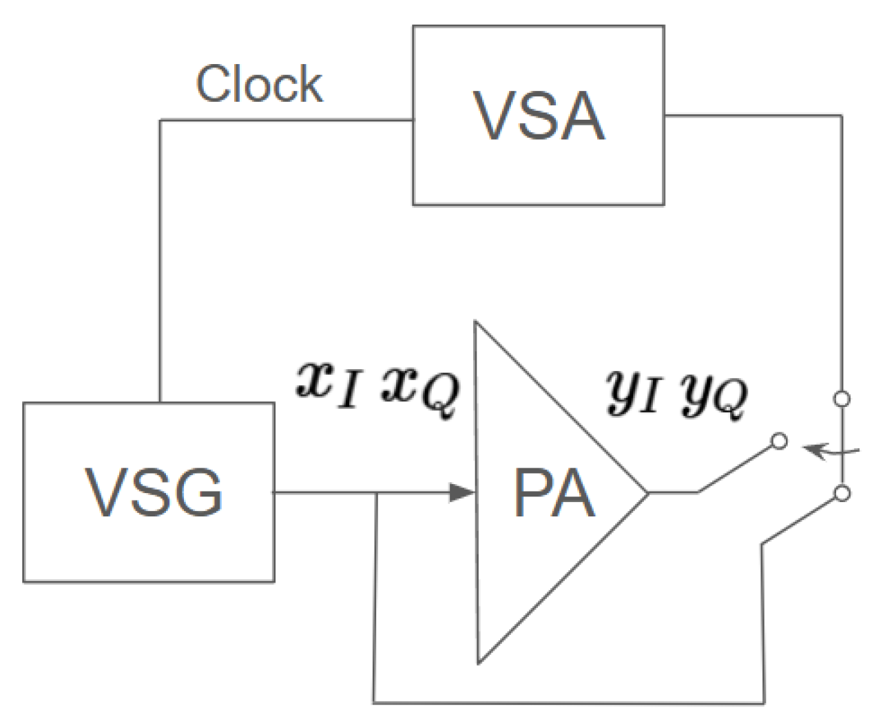
The measurement setup used for PA characterization is depicted in Figure 1. A vector signal generator (VSG) is employed to generate the in-phase and quadrature components ($x_{\mathrm{I}},x_{\mathrm{Q}}$) of the input test signals, and modulated waveforms such as WCDMA. These signals are applied to the power amplifier (PA), which introduces nonlinear distortions and memory effects, producing the output signals ($y_{\mathrm{I}},y_{\mathrm{Q}}$). The output of the PA, as well as the reference input signal, is sequentially captured by the vector signal analyzer (VSA). A shared clock between the VSG and the VSA guarantees synchronization in both time and frequency domains, which is essential for coherent acquisition.

For $PV$ and $2D\text{-}PV$ models, the identification was performed by the least-squares (LS) method. In the case of the $2D\text{-}frPV$ model, the identification was carried out by the LS method and by a nonlinear optimization algorithm named fmincon, used to optimize and find the local minimum of the function $OF$ within a nonlinear optimization with a constraint on the $\alpha$ values. These two steps were performed in MATLAB R2015a (Student Version), licensed for academic use, using double precision floating point arithmetic.

The normalized mean square error ($NMSE$) metric was used to measure the accuracy of the three models. In this metric, the calculation is performed on the error signals defined by the differences between the signals measured at the output of the RF PA and the signals estimated at the output of the different models, as follows:

$$NMSE=10lo{g}_{10}\left[{\displaystyle \frac{{\sum }_{i=1}^N{\left|{\tilde{y}}_{measured}\left(i\right)-{\tilde{y}}_{estimated}\left(i\right)\right|}^2}{{\sum }_{i=1}^N{\left|{\tilde{y}}_{measured}\left(i\right)\right|}^2}}\right],$$

(32)

where i specifies a sample and N is the total number of samples, $y_{measured}\left(i\right)$ is the output complex-valued envelope signal measured at the instant i, and $y_{estimated}\left(i\right)$ is the output complex-valued envelope signal estimated by the RF PA models at the instant i. All $NMSE$ values will be expressed in decibels ($\mathrm{dB}$), and the simulation results will be presented in terms of the validation data.

Two scenarios are considered to evaluate the performance of the proposed $2D\text{-}frPV$ model, with analyses conducted for all three devices under test (DUTs). The first scenario focuses on a comparison between the conventional $PV$ and the $2D\text{-}PV$ models, employing two distinct analysis approaches. In the first approach, the goal is to identify configurations in which both models achieve similar $NMSE$ values, but the $2D\text{-}PV$ model requires significantly fewer parameters—thereby highlighting its capacity for parameter reduction. In the second approach, the comparison is made for configurations with the same number of parameters in both models, emphasizing the potential $NMSE$ improvement obtained by adopting a two-dimensional modeling structure.

The second scenario is dedicated to comparing the two-dimensional models ($2D\text{-}PV$ and $2D\text{-}frPV$). This analysis investigates their $NMSE$ performance under equal model complexity (i.e., identical number of parameters). In addition, AM-AM and AM-PM conversion curves derived from the output signals of the three DUTs are analyzed, allowing for a qualitative evaluation of how effectively each model captures the nonlinear amplitude and phase behavior of the RF power amplifier.

In both investigations, to satisfy the conditions of stability in the $2D\text{-}frPV$ model, $\beta$ was defined as $\beta =1$ and the fractional order $\alpha$ was considered within the range $0<\alpha <1$. The range $1<\alpha <2$ was not considered because the $2D\text{-}frPV$ model was not effective enough for fractional orders located within the analyzed range.

In terms of truncation in the $PV$, $2D\text{-}PV$, and $2D\text{-}frPV$ models, each has four freely selected truncation factors. $P_1$ is the truncation factor for the amplitude polynomial order of the three models. $P_2$ is the phase polynomial truncation order of the $PV$ model, while in the $2D\text{-}PV$ and $2D\text{-}frPV$ models, the phase polynomial truncation is $P_3$. M and L are, respectively, the truncation for the amplitude and the phase memories in the $PV$ and $2D\text{-}PV$ models, while in the $2D\text{-}frPV$ model, they are represented by K and Q, respectively. To obtain the simulation results of the direct and inverse RF PA models, the maximum values of the truncation factors in Equations (6), (7) and (28) were defined as $P_1=5$, $P_2=P_3=3$, $M=K=2$ and $L=Q=1$. For these three models, several instances were implemented, where the values of the four truncations vary between their minima and maxima. When all truncation values reach their maximum, $P_1=5$, $P_2=P_3=3$, $M=K=2$ and $L=Q=1$, each model generates a total of 204 parameters.

4.1. GaN HEMT Class AB Power Amplifier

The first device under test ($DU{T}_1$) is a GaN HEMT Class AB radio-frequency power amplifier (RF PA), excited by a 900 MHz carrier modulated by a 3GPP WCDMA envelope signal with a bandwidth of 3.84 MHz. The input and output signals were measured using a Rohde & Schwarz FSQ vector signal analyzer (VSA) operating at a sampling frequency of 30.72 MHz. Prior to modeling, the measured signals were normalized. A total of 3320 samples were used for model identification, and 2100 for validation.

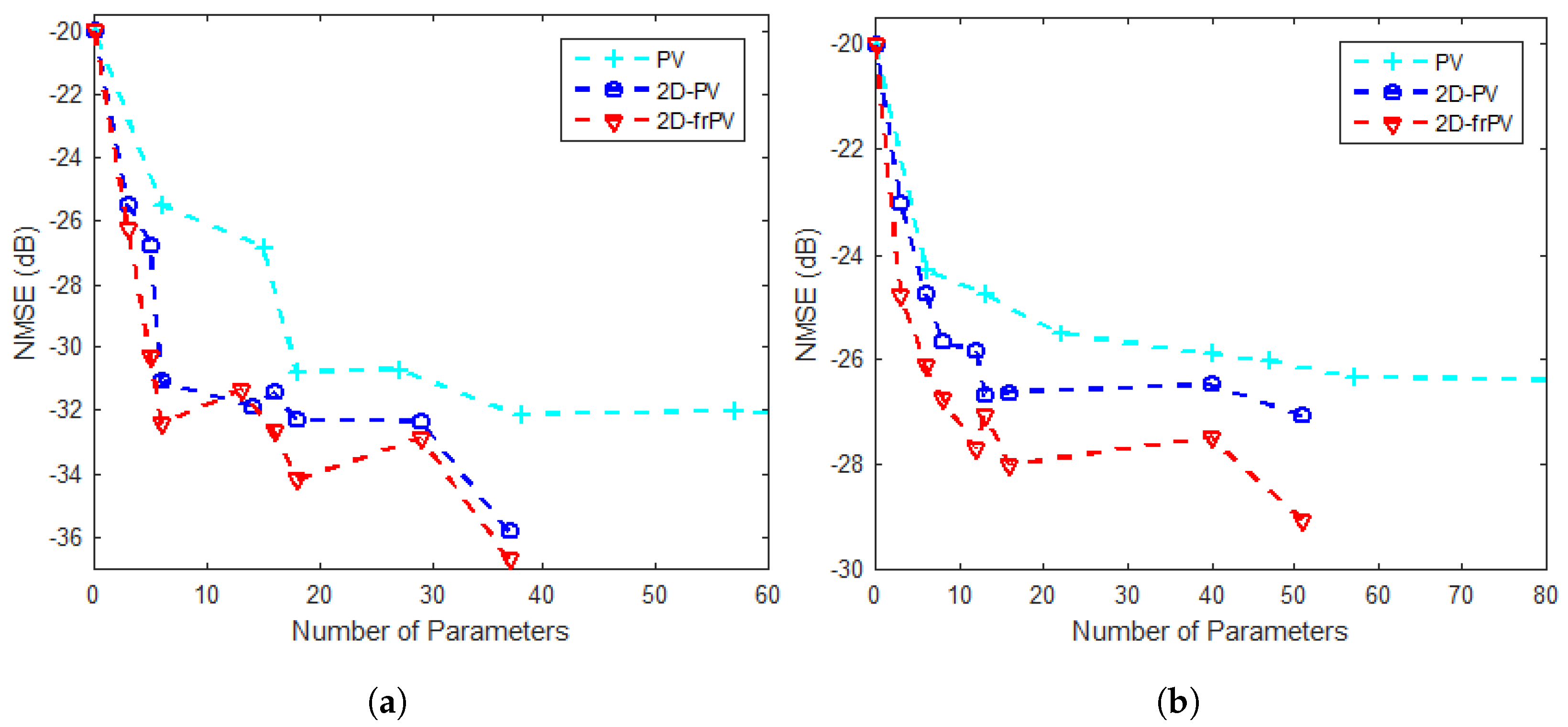
The modeling performance of the $PV$, $2D\text{-}PV$, and $2D\text{-}frPV$ models was evaluated using complex-valued envelope signals represented in polar coordinates. Figure 2 and

Table 1. Comparison of NMSE values, in dB, as a function of the number of parameters for RF PA modeling using $DU{T}_1$.

Model $\mathit{P}\mathit{V}$	Model $2\mathit{D}\text{-}\mathit{P}\mathit{V}$	Model $2\mathit{D}\text{-}\mathit{f}\mathit{r}\mathit{P}\mathit{V}$
(Params/NMSE)	(Params/NMSE)	(Params/NMSE)
81/$-35.31$	37/$-36.02$	37/$-36.70$
68/$-32.26$	29/$-32.36$	29/$-32.88$
57/$-32.02$	18/$-32.30$	18/$-34.17$
38/$-32.15$	16/$-31.45$	16/$-32.66$
27/$-30.71$	14/$-31.87$	14/$-31.34$
18/$-30.79$	6/$-31.09$	6/$-32.42$
15/$-26.80$	5/$-26.73$	5/$-30.31$
6/$-25.49$	3/$-25.49$	3/$-26.25$

Note: Rows highlighted in blue indicate the configurations used for direct NMSE comparison under the same number of parameters across models.

and

Table 2. Comparison of NMSE values, in dB, as a function of the number of parameters for inverse RF PA modeling using $DU{T}_1$.

Model $\mathit{P}\mathit{V}$	Model $2\mathit{D}\text{-}\mathit{P}\mathit{V}$	Model $2\mathit{D}\text{-}\mathit{f}\mathit{r}\mathit{P}\mathit{V}$
(Params/NMSE)	(Params/NMSE)	(Params/NMSE)
105/$-28.22$	51/$-27.08$	51/$-29.06$
81/$-26.41$	40/$-26.48$	40/$-27.48$
57/$-26.35$	16/$-26.64$	16/$-28.01$
47/$-26.03$	13/$-26.69$	13/$-27.08$
40/$-25.90$	12/$-25.85$	12/$-27.69$
22/$-25.51$	8/$-25.68$	8/$-26.77$
13/$-24.72$	6/$-24.74$	6/$-26.12$
6/$-24.28$	3/$-23.02$	3/$-24.76$

Note: Rows highlighted in blue indicate the configurations used for direct NMSE comparison under the same number of parameters across models.

present the Normalized Mean Squared Error (NMSE) as a function of the number of model parameters for both forward modeling (RF PA) and inverse modeling (inv RF PA). These initial results allow for a direct comparison between models under different complexity levels.

The $2D\text{-}PV$ and $2D\text{-}frPV$ models achieved significantly better accuracy with substantially fewer parameters when compared to the conventional Polar Volterra ($PV$) model. For RF PA modeling (Table 1), the number of coefficients was reduced from 57 ($PV$) to 18 ($2D\text{-}PV$ and $2D\text{-}frPV$), corresponding to a 68.4% reduction. In the inverse RF PA modeling scenario (Table 2), the coefficient count was reduced from 47 to 13, resulting in a 72.3% reduction.

Figure 2 serves as visual support for the results presented in Table 1 and Table 2, providing a quick overview of the modeling performance achieved by the $PV$, $2D\text{-}PV$, and $2D\text{-}frPV$ models when applied to $DU{T}_1$. By visual inspection, one can immediately identify the superior performance of the proposed model in achieving lower NMSE values with fewer parameters.

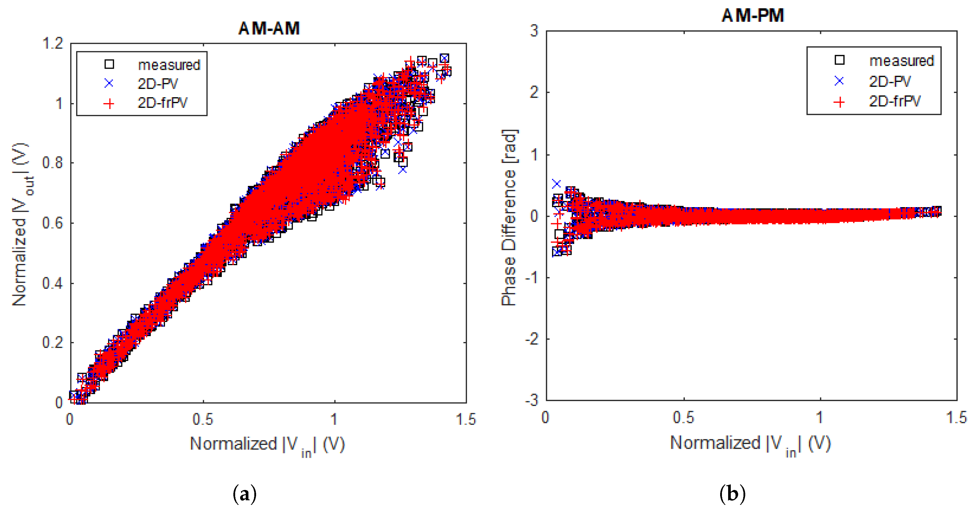
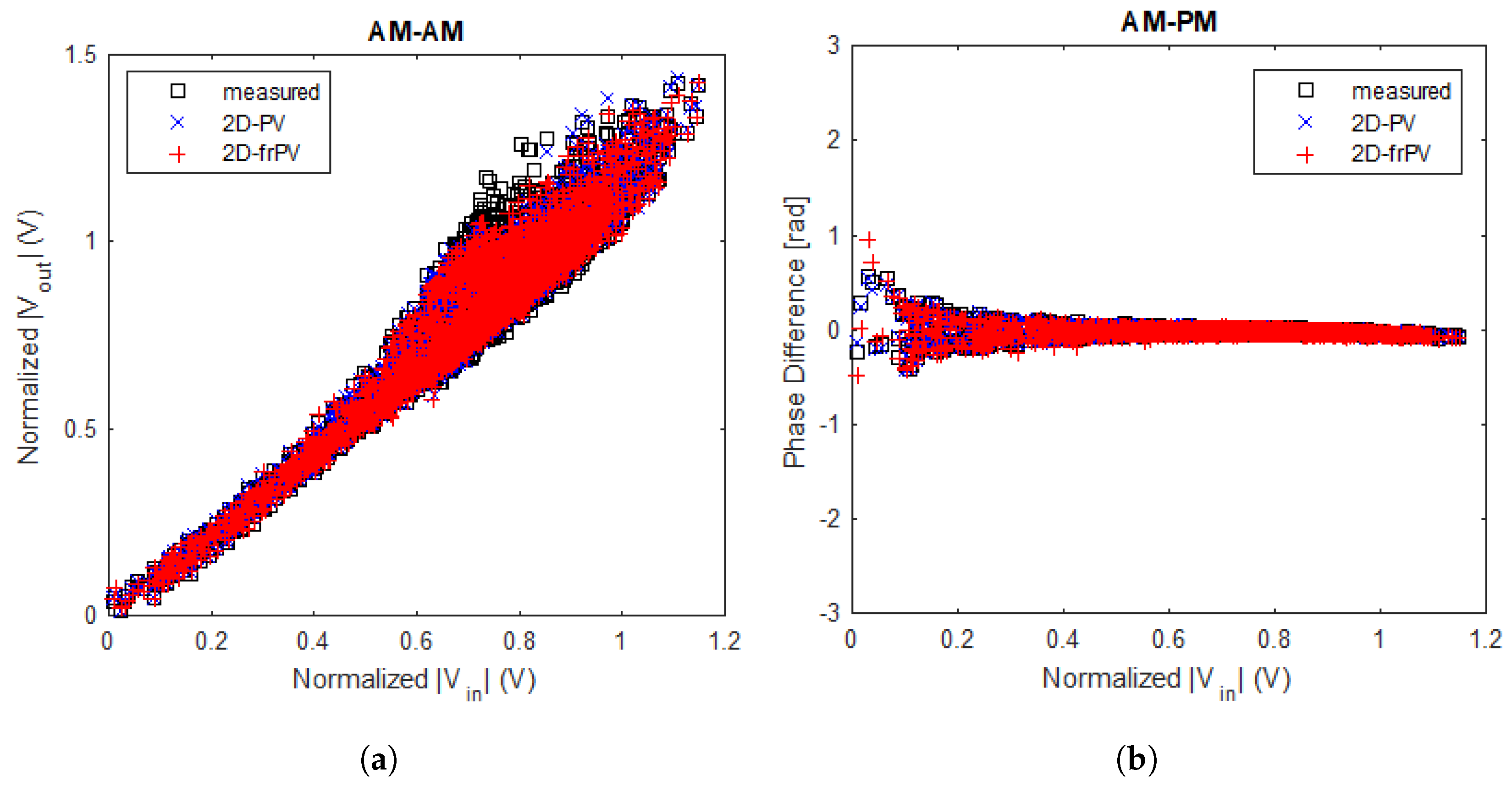
To better understand the value added by the proposed $2D\text{-}frPV$ model, Figure 3 and Figure 4 present the dynamic AM-AM and AM-PM characteristics of the RF PA and inverse RF PA. These results confirm that both $2D\text{-}PV$ and $2D\text{-}frPV$ models are capable of accurately modeling the nonlinear amplitude and phase behavior of $DU{T}_1$.

To further assess the effectiveness of the proposed $2D\text{-}frPV$ model under equal model complexity,

Table 3. Comparison of NMSE values, in dB, as a function of the number of parameters for RF PA modeling using $2D\text{-}PV$ and $2D\text{-}frPV$ models with $DU{T}_1$.

Number of Parameters	$2\mathit{D}\text{-}\mathit{P}\mathit{V}$ (NMSE)	$2\mathit{D}\text{-}\mathit{f}\mathit{r}\mathit{P}\mathit{V}$ (NMSE)
88	$-28.19$	$-32.27$
82	$-28.73$	$-36.23$
56	$-28.22$	$-32.13$
42	$-28.37$	$-32.55$
22	$-27.80$	$-32.59$
12	$-28.24$	$-33.34$
11	$-27.34$	$-32.70$
7	$-24.32$	$-30.99$

Note: The largest observed NMSE gain achieved by the $2D$-$frPV$ model over the $2D$-$PV$ structure was 7.50 dB, for 82 parameters (highlighted row).

and

Table 4. Comparison of NMSE values, in dB, as a function of the number of parameters for the inverse RF PA using $2D\text{-}PV$ and $2D\text{-}frPV$ models with $DU{T}_1$.

Number of Parameters	$2\mathit{D}\text{-}\mathit{P}\mathit{V}$ (NMSE)	$2\mathit{D}\text{-}\mathit{f}\mathit{r}\mathit{P}\mathit{V}$ (NMSE)
82	$-26.68$	$-28.72$
60	$-26.59$	$-30.15$
51	$-27.08$	$-29.06$
42	$-26.31$	$-27.60$
22	$-25.67$	$-28.20$
11	$-25.24$	$-27.45$
7	$-23.07$	$-26.97$
5	$-23.06$	$-26.98$

Note: The largest observed NMSE gain achieved by the $2D\text{-}frPV$ model over the $2D\text{-}PV$ structure was 3.90 dB, for 7 parameters (highlighted row).

compare the NMSE performance of $2D\text{-}PV$ and $2D\text{-}frPV$ for the same number of generated parameters. In the highlighted rows, the largest improvements achieved for $DU{T}_1$ were up to 7.50 dB with 82 parameters (Table 3) and up to 3.90 dB with 7 parameters (Table 4), validating the superior performance of the proposed approach.

4.2. GaN HEMT Class AB Power Amplifier

The second analyzed $DU{T}_2$ is a GaN HEMT class AB RF PA, excited by a carrier wave of 900 MHz modulated through a two-carrier 3GPP WCDMA envelope signal, each with a bandwidth of 3.84 MHz and spaced by 5 MHz. The input and output data were measured using a Rohde & Schwarz FSQ VSA, with a sampling frequency of 61.44 MHz. The set of 4500 estimation samples and another 4500 validation samples, measured experimentally, were used for identification and validation modeling of the three models: $PV$, $2D\text{-}PV$, and $2D\text{-}frPV$.

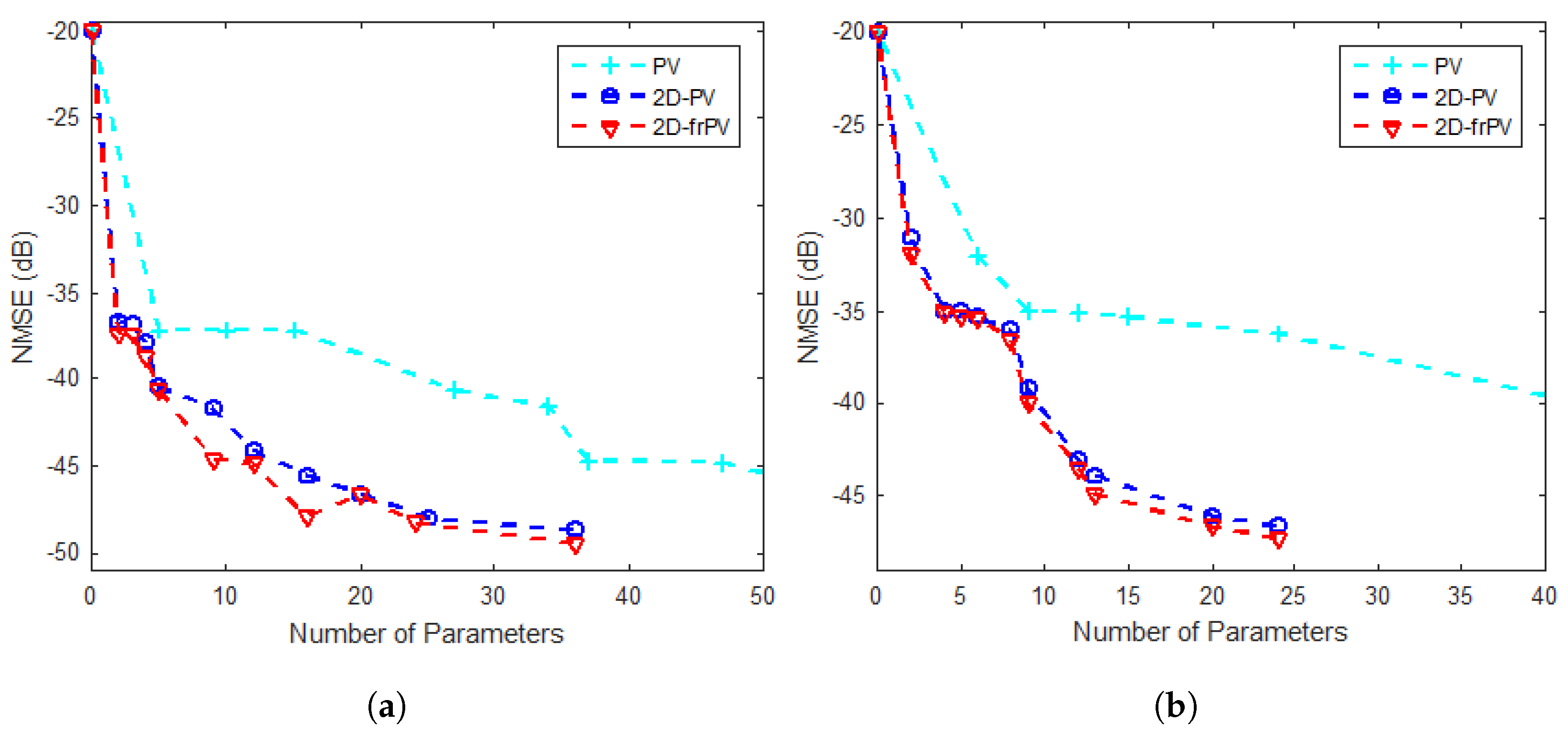
Figure 5, together with

Table 5. Comparison of NMSE values, in dB, as a function of the number of parameters for RF PA modeling using $DU{T}_2$.

Model $\mathit{P}\mathit{V}$	Model $2\mathit{D}\text{-}\mathit{P}\mathit{V}$	Model $2\mathit{D}\text{-}\mathit{f}\mathit{r}\mathit{P}\mathit{V}$
(Params/NMSE)	(Params/NMSE)	(Params/NMSE)
104/$-41.73$	51/$-40.66$	51/$-41.89$
46/$-40.78$	19/$-38.21$	19/$-40.85$
38/$-37.10$	16/$-36.66$	16/$-39.27$
22/$-37.09$	13/$-37.90$	13/$-39.03$
20/$-28.37$	8/$-28.46$	8/$-31.44$
12/$-27.09$	6/$-28.44$	6/$-31.07$
10/$-28.45$	4/$-29.58$	4/$-30.22$
4/$-20.47$	2/$-20.47$	2/$-21.90$

Note: Rows highlighted in blue indicate the configurations used for direct NMSE comparison under the same number of parameters across models.

and

Table 6. Comparison of NMSE values, in dB, as a function of the number of parameters for the inverse RF PA modeling using $DU{T}_2$.

Model $\mathit{P}\mathit{V}$	Model $2\mathit{D}\text{-}\mathit{P}\mathit{V}$	Model $2\mathit{D}\text{-}\mathit{f}\mathit{r}\mathit{P}\mathit{V}$
(Params/NMSE)	(Params/NMSE)	(Params/NMSE)
184/$-36.77$	88/$-35.47$	88/$-36.96$
101/$-35.77$	72/$-35.33$	72/$-35.55$
81/$-35.68$	56/$-35.05$	56/$-34.65$
60/$-31.16$	24/$-31.24$	24/$-34.49$
42/$-31.03$	20/$-31.08$	20/$-34.19$
27/$-30.51$	11/$-30.70$	11/$-31.58$
20/$-31.18$	9/$-30.64$	9/$-31.54$
16/$-30.27$	6/$-30.38$	6/$-31.77$
9/$-24.97$	4/$-25.35$	4/$-25.36$

Note: Rows highlighted in blue indicate the configurations used for direct NMSE comparison under the same number of parameters across models.

, presents the results obtained for RF PA and the inverse RF PA modeling using $DU{T}_2$. The $2D\text{-}PV$ and $2D\text{-}frPV$ models achieve similar or better accuracy than the conventional $PV$ model, using significantly fewer parameters. In RF PA modeling (Table 5), the number of coefficients was reduced by over 60.9% (from 46 to 19), while in the inverse RF PA modeling (Table 6), the reduction reached 62.5% (from 16 to 6 coefficients).

In the highlighted rows, corresponding to equal parameter counts (4 and 9), both $2D$ models clearly outperform the $PV$ baseline. The proposed model shows NMSE improvements of 9.75 dB and 6.58 dB, respectively.

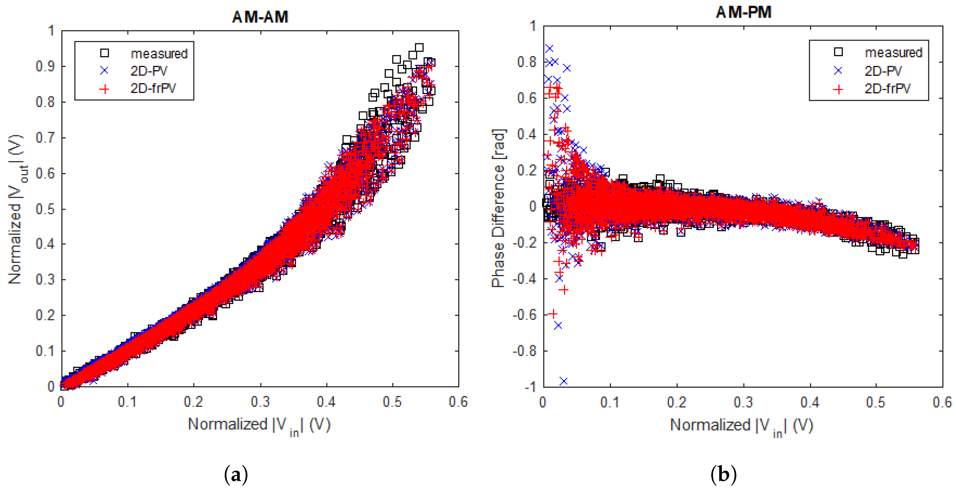
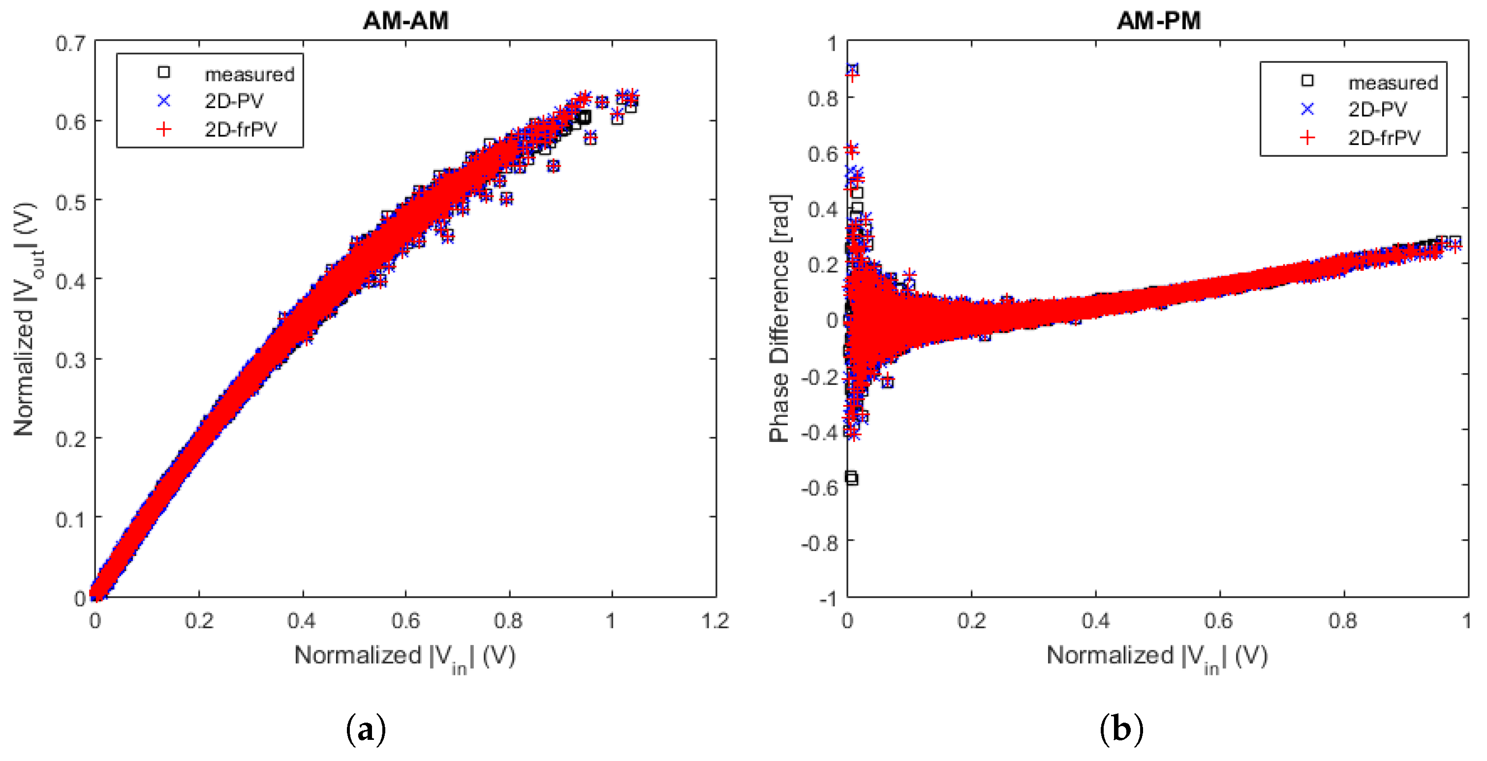
Figure 6 and Figure 7 illustrate the AM-AM and AM-PM characteristics of $DU{T}_2$, estimated using the $2D\text{-}PV$ and $2D\text{-}frPV$ models. Despite the presence of pronounced nonlinearities and memory effects, both models track the dynamic distortions accurately. The similarity between curves confirms the effectiveness of both models in capturing the forward and inverse behaviors of the PA system.

Table 7. Comparison of NMSE values, in dB, as a function of the number of parameters for RF PA modeling using $2D\text{-}PV$ and $2D\text{-}frPV$ models with $DU{T}_2$.

Number of Parameters	$2\mathit{D}\text{-}\mathit{P}\mathit{V}$ (NMSE)	$2\mathit{D}\text{-}\mathit{f}\mathit{r}\mathit{P}\mathit{V}$ (NMSE)
42	$-37.17$	$-38.44$
21	$-37.19$	$-39.80$
19	$-38.21$	$-40.85$
16	$-36.66$	$-39.27$
13	$-37.90$	$-39.03$
12	$-35.59$	$-40.00$
10	$-27.10$	$-31.53$
6	$-28.44$	$-31.07$

Note: The largest observed NMSE gain achieved by the $2D$-$frPV$ model over the $2D$-$PV$ structure was 4.43 dB, for 10 parameters (highlighted row).

and

Table 8. Comparison of NMSE values, in dB, as a function of the number of parameters for the inverse RF PA modeling using $2D\text{-}PV$ and $2D\text{-}frPV$ models with $DU{T}_2$.

Number of Parameters	$2\mathit{D}\text{-}\mathit{P}\mathit{V}$ (NMSE)	$2\mathit{D}\text{-}\mathit{f}\mathit{r}\mathit{P}\mathit{V}$ (NMSE)
45	$-32.42$	$-35.79$
24	$-31.24$	$-34.49$
20	$-31.08$	$-34.19$
19	$-31.48$	$-35.15$
16	$-31.40$	$-34.04$
13	$-33.69$	$-35.10$
6	$-30.38$	$-31.77$

Note: The largest observed NMSE gain achieved by the $2D$-$frPV$ model over the $2D$-$PV$ structure was 3.67 dB, for 19 parameters (highlighted row).

provide a refined comparison between the $2D\text{-}PV$ and $2D\text{-}frPV$ models under matched parameter constraints. In RF PA modeling (Table 7), the largest NMSE improvement reached 4.43 dB with 10 parameters. For the inverse RF PA modeling (Table 8), a 3.67 dB gain was achieved with 19 parameters. These results reinforce the effectiveness of the fractional-order structure introduced in the $2D\text{-}frPV$ model.

4.3. GaN Class AB Power Amplifier

The third and final device under test, $DU{T}_3$, is a GaN class AB RF power amplifier excited by a single-carrier 3GPP WCDMA envelope signal at 900 MHz, with 3.84 MHz bandwidth. The input and output signals were measured using a Rohde & Schwarz FSQ VSA operating at a sampling frequency of 61.44 MHz. A total of 29,550 estimation samples and 8699 validation samples were used to identify and validate the $PV$, $2D\text{-}PV$, and $2D\text{-}frPV$ models.

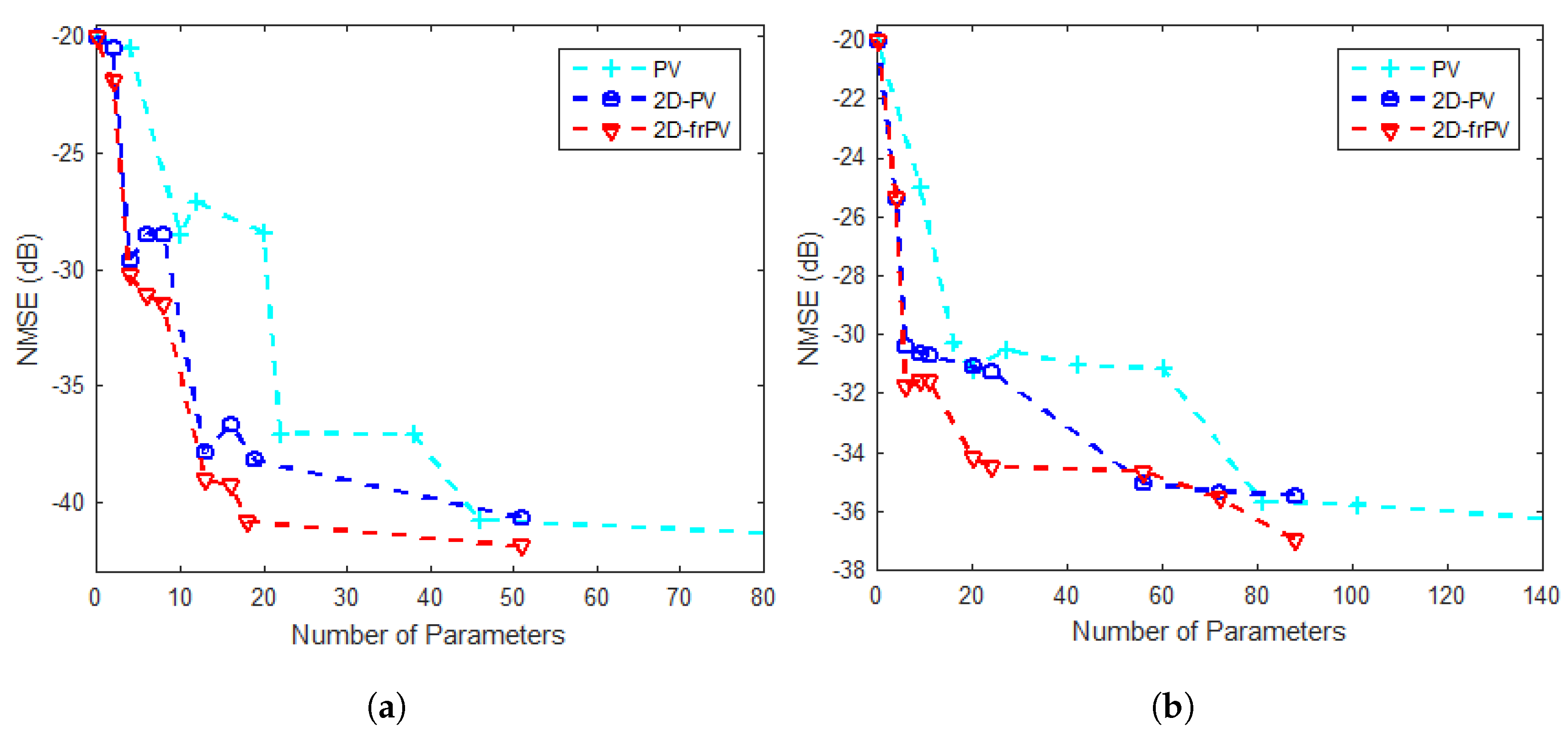
Figure 8 summarizes the NMSE results as a function of the number of parameters for both forward modeling (RF PA) and inverse modeling, using the complex envelope signals obtained from $DU{T}_3$.

In the RF PA modeling scenario, the $2D\text{-}PV$ and $2D\text{-}frPV$ models achieved comparable or superior NMSE performance using significantly fewer coefficients than the $PV$ model. For example, as shown in the seventh row of

Table 9. Comparison of NMSE values, in dB, as a function of the number of parameters for RF PA modeling using $DU{T}_3$.

Model $\mathit{P}\mathit{V}$	Model $2\mathit{D}\text{-}\mathit{P}\mathit{V}$	Model $2\mathit{D}\text{-}\mathit{f}\mathit{r}\mathit{P}\mathit{V}$
(Params/NMSE)	(Params/NMSE)	(Params/NMSE)
105/$-48.49$	36/$-48.69$	36/$-49.44$
64/$-47.05$	25/$-47.99$	25/$-48.22$
57/$-46.69$	20/$-46.59$	20/$-46.69$
47/$-44.82$	16/$-45.55$	16/$-47.90$
37/$-44.71$	12/$-44.11$	12/$-44.85$
34/$-41.57$	9/$-41.69$	9/$-44.61$
27/$-40.66$	5/$-40.50$	5/$-40.69$
15/$-37.17$	4/$-37.89$	4/$-38.82$
10/$-37.16$	3/$-36.75$	3/$-37.44$
5/$-37.16$	2/$-36.71$	2/$-37.38$

Note: Rows highlighted in blue indicate the configurations used for direct NMSE comparison under the same number of parameters across models.

, the number of parameters decreased from 27 in the $PV$ model to just 5 in the two proposed models, representing a reduction of approximately 81.5%, while maintaining similar NMSE values. Similarly, in the inverse RF PA modeling case (

Table 10. Comparison of NMSE values, in dB, as a function of the number of parameters for the inverse RF PA modeling using $DU{T}_3$.

Model $\mathit{P}\mathit{V}$	Model $2\mathit{D}\text{-}\mathit{P}\mathit{V}$	Model $2\mathit{D}\text{-}\mathit{f}\mathit{r}\mathit{P}\mathit{V}$
(Params/NMSE)	(Params/NMSE)	(Params/NMSE)
101/$-46.06$	24/$-46.60$	24/$-47.29$
64/$-45.22$	20/$-46.06$	20/$-46.60$
57/$-44.73$	13/$-43.90$	13/$-44.87$
47/$-43.19$	12/$-43.07$	12/$-43.53$
42/$-40.02$	9/$-39.25$	9/$-40.02$
24/$-36.28$	8/$-36.00$	8/$-36.62$
15/$-35.26$	6/$-35.32$	6/$-35.36$
12/$-35.10$	5/$-35.03$	5/$-35.27$
9/$-34.96$	4/$-35.01$	4/$-35.12$
6/$-32.00$	2/$-31.95$	2/$-31.98$

Note: Rows highlighted in blue indicate the configurations used for direct NMSE comparison under the same number of parameters across models.

), a comparable NMSE was obtained with only 9 parameters in the proposed models, compared to 42 in the $PV$ model, resulting in a 78.6% reduction in model complexity.

A more direct comparison of NMSE performance under the same model complexity is presented in the highlighted rows of Table 9 (5 parameters) and Table 10 (9 parameters). In these configurations, both the $2D$-$PV$ and $2D\text{-}frPV$ models surpass the $PV$ model. Specifically, the proposed $2D$-$frPV$ model achieved NMSE improvements of 3.54 dB in RF PA modeling and 5.06 dB in the inverse RF PA modeling.

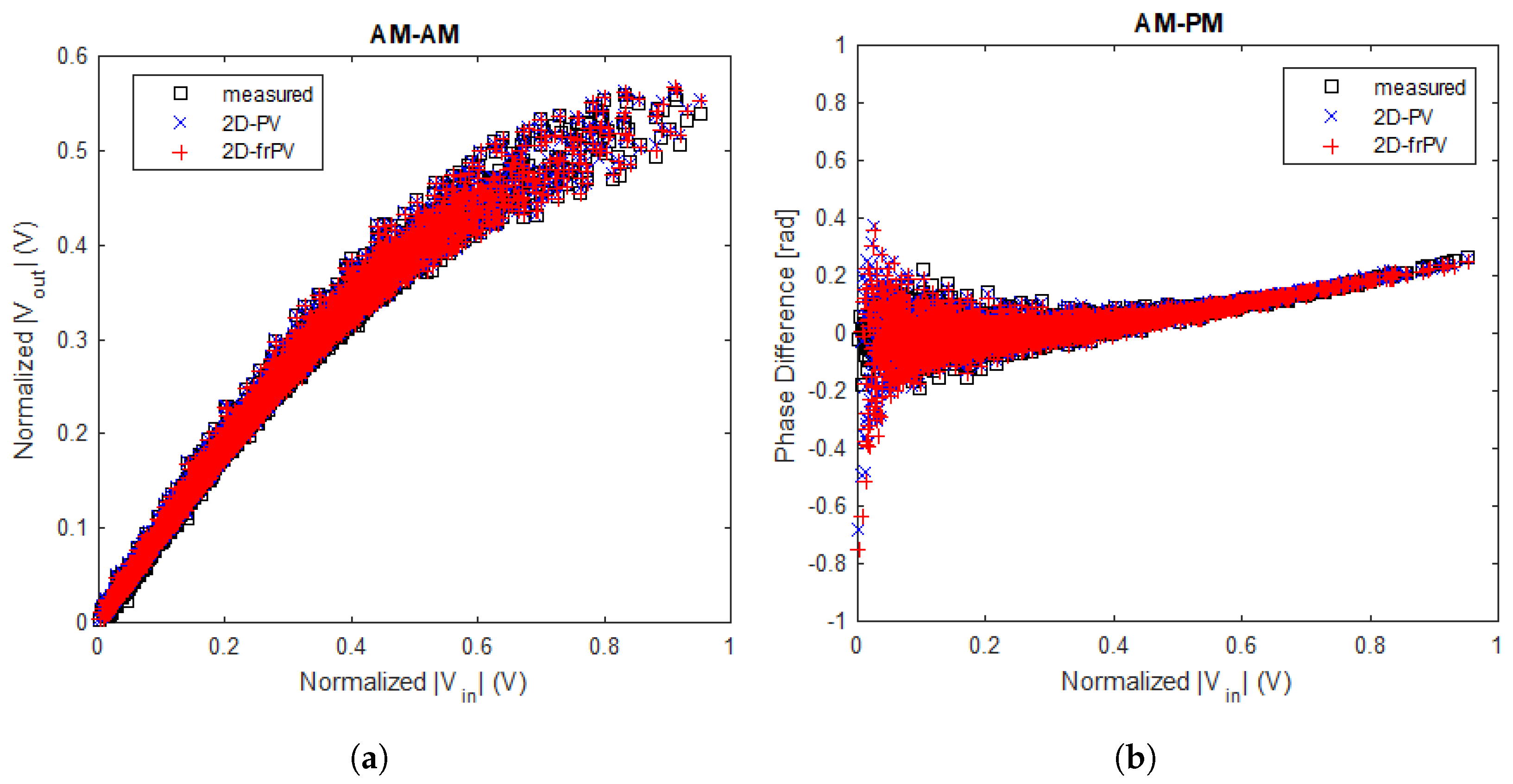
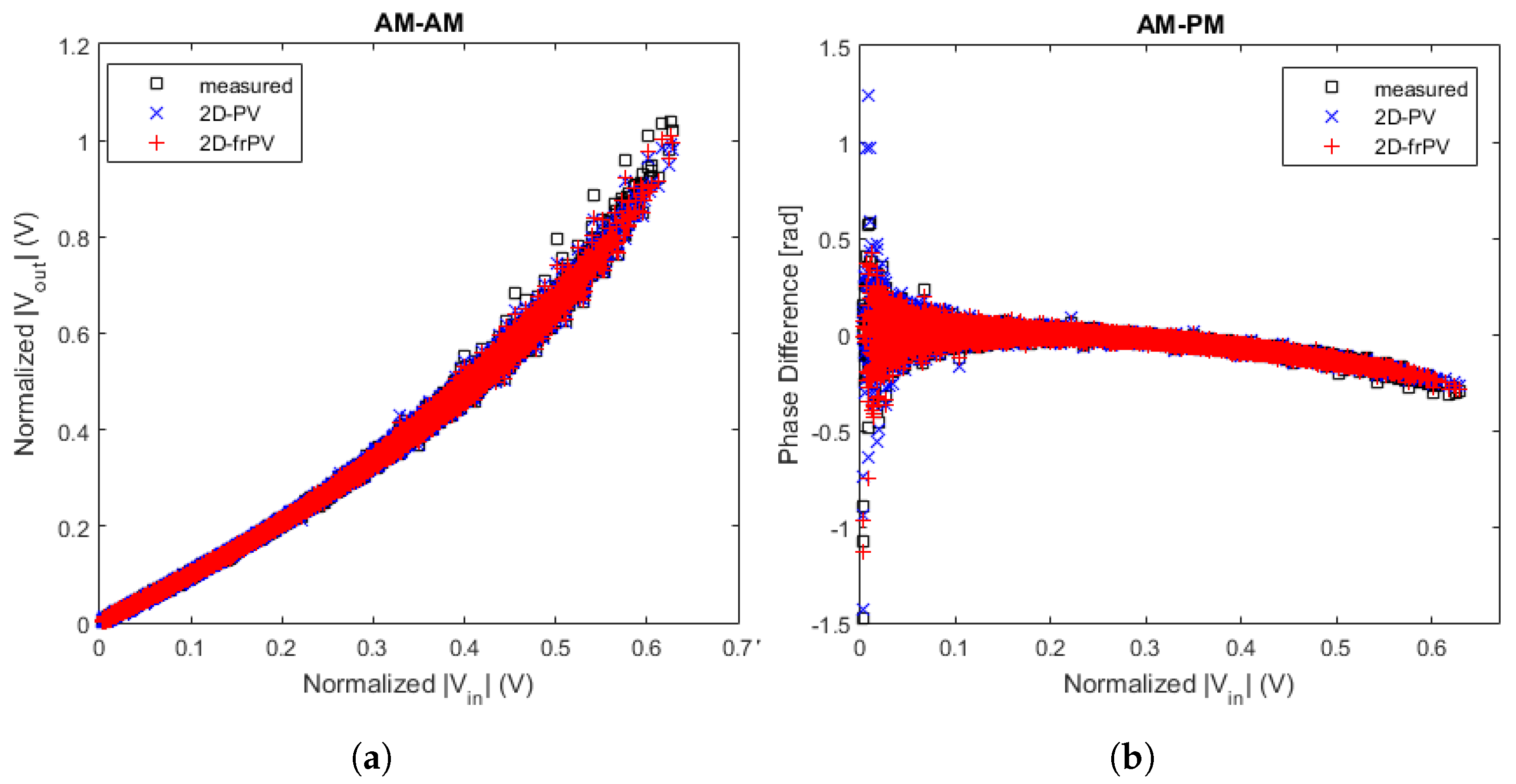
Figure 9 and Figure 10 depict the AM-AM and AM-PM characteristics derived from forward and inverse modeling, respectively. Despite the presence of nonlinearities and phase distortions in the measured signals, both the $2D\text{-}PV$ and $2D\text{-}frPV$ models exhibit consistent behavior and accurately replicate the observed transfer characteristics, supporting the effectiveness of the proposed structure.

Finally,

Table 11. Comparison of the NMSEs of RF PA modeling for $2D\text{-}PV$ and $2D\text{-}frPV$ using $DU{T}_3$.

Number of Parameters	$2\mathit{D}\text{-}\mathit{P}\mathit{V}$ (NMSE)	$2\mathit{D}\text{-}\mathit{f}\mathit{r}\mathit{P}\mathit{V}$ (NMSE)
56	−47.0640	−50.2298
45	−42.2150	−49.5460
39	−42.0328	−45.8290
11	−39.2786	−41.7716
9	−41.6903	−44.6099
7	−37.2342	−40.7974
6	−37.9297	−40.6009

Note: The largest observed NMSE gain achieved by the $2D$-$frPV$ model over the $2D$-$PV$ structure was 7.33 dB, for 45 parameters (highlighted row).

and

Table 12. Comparison of the NMSEs of the inverse RF PA modeling for $2D\text{-}PV$ and $2D\text{-}frPV$ using $DU{T}_3$.

Number of Parameters	$2\mathit{D}\text{-}\mathit{P}\mathit{V}$ (NMSE)	$2\mathit{D}\text{-}\mathit{f}\mathit{r}\mathit{P}\mathit{V}$ (NMSE)
59	−40.9558	−49.6751
39	−40.9025	−45.3848
28	−41.0013	−46.0661
18	−40.5022	−45.7576
16	−40.8712	−45.7331
10	−36.5216	−43.3250

Note: The largest observed NMSE gain achieved by the $2D$-$frPV$ model over the $2D$-$PV$ structure was 8.72 dB, for 59 parameters (highlighted row).

provide a more detailed comparison between the two $2D$ models. The largest observed NMSE gain achieved by the $2D\text{-}frPV$ model over the $2D\text{-}PV$ structure was 7.33 dB in RF PA modeling (Table 11, 45 parameters), and 8.72 dB in the inverse RF PA modeling (Table 12, 59 parameters), further demonstrating the advantages of incorporating fractional-order dynamics in two-dimensional modeling frameworks.

5. Discussion

This work proposes an approach using a two-dimensional fractional Polar Volterra expansion model that significantly reduces the number of parameters to be estimated and substantially improves the accuracy of RF PA behavioral modeling in comparison with the previous two-dimensional Polar Volterra and Polar Volterra series models. It can accurately reproduce nonlinear distortions of the highly efficient wideband RF PA with long-term memory effects. The extraction of the proposed $2D\text{-}frPV$ model is simple and was carried out using three different devices under test. Compared to the $PV$ model, both $2D\text{-}PV$ and $2D\text{-}frPV$ models provide a reduction of the number of generated parameters in the model by more than 81.5%. In further comparisons with the $2D\text{-}PV$ model, the proposed two-dimensional fractional Polar Volterra model, $2D\text{-}frPV$, demonstrated a significant enhancement in modeling accuracy for the inverse RF PA modeling, achieving $NMSE$ improvements of up to 8.72 dB. In order to avoid potential ill-conditioning during model extraction, the number of samples was always set to be much larger than the number of coefficients. The complete dataset was divided into two subsets: one used for model extraction and the other exclusively reserved for validation. In all cases, the errors obtained showed very similar behavior when computed on the extraction dataset and on the independent validation dataset, which is an indication that no conditioning issues affected the reported results. To provide a broader perspective on the modeling performance across different scenarios,

Table 13. Summary of parameter reduction (required to achieve similar NMSE performance) and NMSE improvement of the proposed $2D\text{-}frPV$ model in comparison to the conventional $PV$ and $2D$-$PV$ models for all DUTs.

DUT	Parameter Reduction ($\mathit{P}\mathit{V}$ → $2\mathit{D}\text{-}\mathit{f}\mathit{r}\mathit{P}\mathit{V}$)	NMSE Gain vs. $\mathit{P}\mathit{V}$	NMSE Gain vs. $2\mathit{D}\text{-}\mathit{P}\mathit{V}$
DUT1	RF PA: 57 → 18 (↓ 68.4%)	+6.93 dB (6 †)	+7.50 dB (82 †)
	inv: 47 → 13 (↓72.3%)	+2.36 dB (13 †)	+3.90 dB (7 †)
DUT2	RF PA: 46 → 19 (↓60.9%)	+9.75 dB (4 †)	+4.43 dB (10 †)
	inv: 16 → 6 (↓62.7%)	+6.57 dB (9 †)	+3.67 dB (19 †)
DUT3	RF PA: 27 → 5 (↓81.5%)	+3.54 dB (5 †)	+7.33 dB (45 †)
	inv: 42 → 9 (↓78.6%)	+5.06 dB (9 †)	+8.72 dB (59 †)

(↓) the downward arrow indicates the percentage of parameter reduction. ^† Equal number of parameters used for NMSE comparison. Note: The highlighted rows indicate the largest observed parameter reduction and NMSE gain across all analyses. Both occurred for $DU{T}_3$: a parameter reduction of 81.5% and a maximum NMSE improvement of +8.72 dB achieved by the $2D$-$frPV$ model over the $2D$-$PV$ structure with 59 parameters.

summarizes the results obtained for the three devices under test (DUTs). This comparative overview highlights the reduction in model complexity—quantified by the number of parameters—as well as the corresponding improvement in modeling accuracy, measured by the Normalized Mean Squared Error (NMSE). The results reinforce the robustness and generalization capability of the proposed two-dimensional fractional Polar Volterra ($2D$-$frPV$) model, which consistently outperformed the baseline $PV$ and $2D$-$PV$ structures. The observed gains support the hypothesis that incorporating both two-dimensional and fractional-order dynamics yields more efficient and accurate representations of nonlinear power amplifier behavior across diverse experimental conditions.

References

1. Huang, T.; Yang, W.; Wu, J.; Ma, J.; Zhang, X.; Zhang, D. A survey on green 6G network: Architecture and technologies. IEEE Access 2019, 7, 175758–175768. [Google Scholar] [CrossRef]
2. Wolff, N.; Chevtchenko, S.; Wentzel, A.; Bengtsson, O.; Heinrich, W. Switch-type modulators and PAs for efficient transmitters in the 5G wireless infrastructure. In Proceedings of the 2018 IEEE MTT-S International Microwave Workshop Series on 5G Hardware and System Technologies (IMWS-5G), Dublin, Ireland, 30–31 August 2018; pp. 1–3. [Google Scholar]
3. Cho, Y.; Lee, W.; Park, H.c.; Park, B.; Lee, J.H.; Kim, J.; Lee, J.; Kim, S.; Park, J.; Park, S.; et al. A 16-element phased-array CMOS transmitter with variable gain controlled linear power amplifier for 5G new radio. In Proceedings of the 2019 IEEE Radio Frequency Integrated Circuits Symposium (RFIC), Boston, MA, USA, 2–4 June 2019; pp. 247–250. [Google Scholar]
4. Popovic, Z. Amping up the PA for 5G: Efficient GaN power amplifiers with dynamic supplies. IEEE Microw. Mag. 2017, 18, 137–149. [Google Scholar] [CrossRef]
5. Sun, J.; Shi, W.; Yang, Z.; Yang, J.; Gui, G. Behavioral modeling and linearization of wideband RF power amplifiers using BiLSTM networks for 5G wireless systems. IEEE Trans. Veh. Technol. 2019, 68, 10348–10356. [Google Scholar] [CrossRef]
6. Roblin, P.; Root, D.E.; Verspecht, J.; Ko, Y.; Teyssier, J.P. New trends for the nonlinear measurement and modeling of high-power RF transistors and amplifiers with memory effects. IEEE Trans. Microw. Theory Tech. 2012, 60, 1964–1978. [Google Scholar] [CrossRef]
7. Park, C.S.; Sundström, L.; Wallén, A.; Khayrallah, A. Carrier aggregation for LTE-advanced: Design challenges of terminals. IEEE Commun. Mag. 2013, 51, 76–84. [Google Scholar] [CrossRef]
8. Han, G.; Yang, X.; Liu, L.; Chan, S.; Zhang, W. A coverage-aware hierarchical charging algorithm in wireless rechargeable sensor networks. IEEE Netw. 2018, 33, 201–207. [Google Scholar] [CrossRef]
9. Álvarez-López, L.; Becerra, J.A.; Madero-Ayora, M.J.; Crespo-Cadenas, C. Determining a Digital Predistorter Model Structure for Wideband Power Amplifiers through Random Forest. In Proceedings of the 2020 IEEE Topical Conference on RF/Microwave Power Amplifiers for Radio and Wireless Applications (PAWR), San Antonio, TX, USA, 26–29 January 2020; pp. 50–52. [Google Scholar]
10. Özgül, B.; Langer, J.; Noguera, J.; Vissers, K. Software-programmable digital pre-distortion on new generation FPGAs. Analog Integr. Circuits Signal Process. 2014, 78, 573–587. [Google Scholar] [CrossRef]
11. Desgreys, P.; Manyam, V.N.; Tchambake, K.; Pham, D.K.G.; Jabbour, C. Wideband power amplifier predistortion: Trends, challenges and solutions. In Proceedings of the 2017 IEEE 12th international conference on ASIC (ASICON), Guiyang, China, 25–28 October 2017; pp. 100–103. [Google Scholar]
12. Kim, J.; Konstantinou, K. Digital predistortion of wideband signals based on power amplifier model with memory. Electron. Lett. 2001, 37, 1417–1418. [Google Scholar] [CrossRef]
13. Morgan, D.R.; Ma, Z.; Kim, J.; Zierdt, M.G.; Pastalan, J. A generalized memory polynomial model for digital predistortion of RF power amplifiers. IEEE Trans. Signal Process. 2006, 54, 3852–3860. [Google Scholar] [CrossRef]
14. Bonfim, E.J.; de Lima, E.G. A modified two dimensional Volterra-based series for the low-pass equivalent behavioral modeling of RF power amplifiers. Prog. Electromagn. Res. M 2016, 47, 27–35. [Google Scholar] [CrossRef]
15. Cunha, T.R.; Lima, E.G.; Pedro, J.C. A polar-oriented Volterra model for power amplifier characterization. In Proceedings of the 2010 IEEE MTT-S International Microwave Symposium, Anaheim, CA, USA, 23–28 May 2010; pp. 556–559. [Google Scholar]
16. Cunha, T.R.; Lima, E.G.; Pedro, J.C. Validation and physical interpretation of the power-amplifier polar Volterra model. IEEE Trans. Microw. Theory Tech. 2010, 58, 4012–4021. [Google Scholar] [CrossRef]
17. Nypwipwy, V.B.; Cavalheiro, R.A.d.S.; Dartora, C.A.; de Lima, E.G. Power amplifier behavioral modeling based on Laguerre Polar-Volterra series with independent truncations. Int. J. RF Microw. Comput.-Aided Eng. 2022, 32, e23104. [Google Scholar] [CrossRef]
18. Mohamed, A.; Malti, R.; Olivier, C.; Oustaloup, A. System identification using fractional Hammerstein models. IFAC Proc. Vol. 2002, 35, 265–269. [Google Scholar] [CrossRef]
19. Benoît-Marand, F.; Signac, L.; Poinot, T.; Trigeassou, J.C. Identification of non linear fractional systems using continuous time neural networks. IFAC Proc. Vol. 2006, 39, 402–407. [Google Scholar] [CrossRef]
20. Chen, J.; Zeng, Z.; Jiang, P. Global Mittag-Leffler stability and synchronization of memristor-based fractional-order neural networks. Neural Netw. 2014, 51, 1–8. [Google Scholar] [CrossRef] [PubMed]
21. Popa, C.A. Mittag–Leffler stability and synchronization of neutral-type fractional-order neural networks with leakage delay and mixed delays. J. Frankl. Inst. 2023, 360, 327–355. [Google Scholar] [CrossRef]
22. Maachou, A.; Malti, R.; Melchior, P.; Battaglia, J.L.; Oustaloup, A.; Hay, B. Nonlinear thermal system identification using fractional Volterra series. Control Eng. Pract. 2014, 29, 50–60. [Google Scholar] [CrossRef]
23. Alomari, A.K.; Alaroud, M.; Tahat, N.; Almalki, A. Extended Laplace Power Series Method for Solving Nonlinear Caputo Fractional Volterra Integro-Differential Equations. Symmetry 2023, 15, 1296. [Google Scholar] [CrossRef]
24. Alabdala, A.T.; Redhwan, S.S.; Aljaaidi, T.A. Existence and approximate solution for the fractional volterra fredholm integro-differential equation involving ζ-hilfer fractional derivative. Nonlinear Funct. Anal. Appl. 2023, 28, 989–1004. [Google Scholar]
25. Lupupa, M.; Hadjiloucas, S. fractional-order system identification and equalization in massive mimo systems. IEEE Access 2020, 8, 86481–86494. [Google Scholar] [CrossRef]
26. Podlubny, I. Fractional Differential Equations: An Introduction to Fractional Derivatives, Fractional Differential Equations, to Methods of Their Solution and Some of Their Applications; Academic Press: San Diego, CA, USA, 1998. [Google Scholar]
27. Caponetto, R. Fractional Order Systems: Modeling and Control Applications; World Scientific: Singapore, 2010; Volume 72. [Google Scholar]
28. Stanisławski, R.; Latawiec, K.J.; Hunek, W.P.; Łukaniszyn, M. Laguerre-based modeling of fractional-order LTI SISO systems. In Proceedings of the 2013 18th International Conference on Methods & Models in Automation & Robotics (MMAR), Miedzyzdroje, Poland, 26–29 August 2013; pp. 610–615. [Google Scholar]
29. Tepljakov, A. Fractional-Order Modeling and Control of Dynamic Systems; Springer: Cham, Switzerland, 2017. [Google Scholar]
30. Schetzen, M. Synthesis of a class of non-linear systems. Int. J. Control 1965, 1, 401–414. [Google Scholar] [CrossRef]
31. Matignon, D. Stability properties for generalized fractional differential systems. In ESAIM: Proceedings; EDP Sciences: Les Ulis, France, 1998; Volume 5, pp. 145–158. [Google Scholar]
32. Malti, R.; Aoun, M.; Levron, F.; Oustaloup, A. Fractional Differentiation and its Applications. In Volume 1–Mathematical Tools, Geometrical and Physical Aspects; Ubooks: Neusäß, Germany, 2005; pp. 87–102. [Google Scholar]
33. Aoun, M.; Malti, R.; Levron, F.; Oustaloup, A. Synthesis of fractional Laguerre basis for system approximation. Automatica 2007, 43, 1640–1648. [Google Scholar] [CrossRef]
34. Matignon, D. Stability results for fractional differential equations with applications to control processing. In Proceedings of the Computational Engineering in Systems Applications (CESA), Lille, France, 9–12 July 1996; Volume 2, pp. 963–968. [Google Scholar]
35. Das, S.; Pan, I. Fractional Order Signal Processing: Introductory Concepts and Applications; Springer Science & Business Media: Berlin/Heidelberg, Germany, 2011. [Google Scholar]
36. Oldham, K.; Spanier, J. The Fractional Calculus Theory and Applications of Differentiation and Integration to Arbitrary Order; Academic Press: New York, NY, USA, 1974. [Google Scholar]
37. Pedro, J.C.; Nunes, L.C. A single-ended power amplifier behavioral model for AM/AM and AM/PM predictions. In Proceedings of the 2014 IEEE Topical Conference on Power Amplifiers for Wireless and Radio Applications (PAWR), Newport Beach, CA, USA, 19–23 January 2014; pp. 79–81. [Google Scholar]
38. Jardón-Aguilar, H.; Tirado-Méndez, J.A.; Galván-Tejada, G.M.; Iturbide-Sanchez, F. The AM-PM conversion model as a phase statement of compression and desensitization in highly linear multicarrier power amplifiers. Int. J. RF Microw. Comput.-Aided Eng. 2006, 16, 588–595. [Google Scholar] [CrossRef]
39. Lima, E.G.; Cunha, T.R.; Pedro, J.C. A physically meaningful neural network behavioral model for wireless transmitters exhibiting PM–AM/PM–PM distortions. IEEE Trans. Microw. Theory Tech. 2011, 59, 3512–3521. [Google Scholar] [CrossRef]
40. Nazari, N.; Haeri, M.; Tavazoei, M.S. Estimating the fractional order of orthogonal rational functions used in the identification. In Proceedings of the 2008 International Conference on Control, Automation and Systems, Seoul, Republic of Korea, 14–17 October 2008; pp. 1130–1134. [Google Scholar]
Figure 1. A conventional measurement arrangement, consisting essentially of a vector signal generator (VSG) and a vector signal analyzer (VSA), used for behavioral power amplifier characterization and modeling.
Electronics 14 03673 g001
Figure 2. Normalized Mean Squared Error ( N M S E ) as a function of the number of parameters for RF PA and inverse RF PA modeling using D U T 1 . The models P V , 2 D - P V , and 2 D - f r P V were identified using complex envelope signals in polar coordinates, experimentally acquired from a GaN HEMT Class AB power amplifier ( D U T 1 ) operating at 900 MHz with a 3.84 MHz WCDMA-modulated input. Panel (a) shows the modeling results of the forward path (RF PA), while panel (b) presents the corresponding results for the inverse RF PA model.
Electronics 14 03673 g002
Figure 3. AM-AM and AM-PM characteristics obtained from the forward modeling of D U T 1 using the P V , 2 D - P V , and 2 D - f r P V models. The input and output complex envelope signals in polar coordinates were experimentally acquired from a GaN HEMT Class AB RF PA excited at 900 MHz with a 3.84 MHz WCDMA-modulated input. Panel (a) shows the amplitude distortion (AM-AM), while panel (b) presents the phase distortion (AM-PM) behavior modeled by each approach.
Electronics 14 03673 g003
Figure 4. AM-AM and AM-PM characteristics obtained from the inverse modeling of D U T 1 using the P V , 2 D - P V , and 2 D - f r P V models. The input and output complex envelope signals in polar coordinates were experimentally acquired from a GaN HEMT Class AB RF PA excited at 900 MHz with a 3.84 MHz WCDMA-modulated input. Panel (a) presents the amplitude distortion (AM-AM), while panel (b) shows the phase distortion (AM-PM) compensated for by each model.
Electronics 14 03673 g004
Figure 5. Normalized Mean Squared Error ( N M S E ) as a function of the number of parameters for RF PA and the inverse RF PA modeling using D U T 2 . (a) Forward modeling (RF PA). (b) Inverse modeling.
Electronics 14 03673 g005
Figure 6. AM-AM and AM-PM characteristics obtained from the forward modeling of D U T 2 using the 2 D - P V and 2 D - f r P V models. (a) Amplitude distortion (AM-AM). (b) Phase distortion (AM-PM).
Electronics 14 03673 g006
Figure 7. AM-AM and AM-PM characteristics obtained from the inverse modeling of D U T 2 using the 2 D - P V and 2 D - f r P V models. (a) Amplitude distortion (AM-AM). (b) Phase distortion (AM-PM) compensated for by each model.
Electronics 14 03673 g007
Figure 8. Normalized Mean Squared Error ( N M S E ) as a function of the number of parameters for RF PA and the inverse RF PA modeling using D U T 3 . (a) Forward modeling (RF PA). (b) Inverse modeling.
Electronics 14 03673 g008
Figure 9. AM-AM and AM-PM characteristics obtained from the forward modeling of D U T 3 using the 2 D - P V and 2 D - f r P V models. (a) Amplitude distortion (AM-AM). (b) Phase distortion (AM-PM).
Electronics 14 03673 g009
Figure 10. AM-AM and AM-PM characteristics obtained from the inverse modeling of D U T 3 using the 2 D - P V and 2 D - f r P V models. (a) Amplitude distortion (AM-AM). (b) Phase distortion (AM-PM).
Electronics 14 03673 g010