Data-Driven Modeling and Control of Wireless Power Transfer Systems

Abstract

This paper proposes a data-driven modeling and control method for wireless power transmission systems. To address problems such as parameter deviation and high-order complexity in traditional circuit-theory-based modeling, this paper adopts the data-driven Petrov-Galerkin projection and the generalized Lyapunov balancing method to obtain a reduced-order model directly from experimental data. This approach formulates quadratic matrix inequalities to characterize the data and noise, enabling the direct design of a reduced-order model without intermediate system identification steps. The resulting model order is reduced to merely 2–4. Furthermore, by constructing the extended state space and solving the algebraic Riccati equation, we design a linear quadratic regulator-proportional integral controller with integral action to eliminate steady-state error. Experimentally, the method proves to be independent of detailed physical models while achieving both high-fidelity modeling and superior control.

1. Introduction

In recent years, with the rapid development of electric vehicles [1,2,3], consumer electronics [4,5,6], healthcare [7,8] and marine industries [9,10], wireless power transfer (WPT) technology has attracted significant attention due to its contactless energy delivery, high safety, and reliability [11]. Particularly in scenarios where frequent plugging/unplugging is inconvenient, or where insulation and dynamic energy supply are required, WPT systems offer flexible, stable, and environmentally friendly solutions. Among them, the induced power transmission discussed in this paper has become the mainstream solution of WPT due to its advantages such as simple structure, mature technology, and electromagnetic compatibility [12].

To achieve efficient and stable energy transfer, WPT systems require accurate modeling techniques and effective control strategies. Numerous modeling methods have been developed to characterize their dynamic behavior. These include the state space model [13,14], the generalized state space mean model [15], the extended description function [16], and modeling approaches based on the dq synchronous rotating coordinate system [17]. However, practical WPT systems typically consist of high-frequency inverters and numerous passive components (such as resistors, capacitors, and inductors). As a result, models derived from these methods often exhibit high complexity and are challenging to simplify. Even under full resonance conditions, the system can only be reduced to a fifth-order differential equation [18]. In recent years, to further improve model simplicity and practicality, researchers have proposed alternative approaches such as the energy balancing method [19], dynamic phasor method [20], and neural network-based machine learning methods [21]. Nevertheless, these approaches still rely to some extent on physical parameters or prior knowledge. Once the operating conditions or parameters change, they may result in a significant reduction in model accuracy, thereby affecting controller design and system performance.

On the control side, various strategies have been proposed, including impedance matching, Buck/Boost regulation, dynamic frequency modulation, and phase-shift control. For output voltage regulation, a common approach is to insert a Buck-Boost circuit between the secondary rectifier and the load [22,23,24]. This method achieves stable regulation through duty-cycle feedback at the cost of additional circuit complexity. In another method, dynamic frequency modulation can be implemented in the inverter circuit to adjust the output voltage [25]. This technique maintains the capacitor terminal voltage via nominal frequency changes; however, it risks shifting the system away from resonant conditions, which increases impedance and degrades conversion efficiency. Another strategy adopts phase-shift full-bridge control to regulate the output voltage through phase-angle adjustments [26]. Although this approach reduces switching losses and extends device lifespan, it inherently limits the flexibility of regulation.

To address these issues, data-driven approaches have recently been introduced into WPT modeling and control. Unlike conventional model-based identification methods, data-driven modeling directly constructs low-order models from input–output data, avoiding complex identification processes [27,28]. Such methods are capable of generating stable, low-dimensional state-space models that retain key dynamic characteristics while preserving interpretability. Building upon these foundations, this paper proposes a novel data-driven modeling approach that relies solely on input-output data and further develops a proportional-integral (PI) control scheme within a linear quadratic regulator (LQR) framework. The proposed modeling method begins by formulating a consistent system set described by the quadratic matrix inequality (QMI) under noisy data constraints. To guarantee stability and achieve order reduction, the approach subsequently employs generalized Lyapunov balancing and Petrov–Galerkin projection. Thereafter, a PI controller is synthesized within the LQR framework. This is achieved by constructing an augmented state-space model and solving the corresponding algebraic Riccati equation. The proposed control strategy ensures closed-loop stability and significantly improves the dynamic response of the system.

This paper proposes a novel data-driven framework for the modeling and control of WPT systems. The primary contributions are:

1.

A data-driven modeling framework for WPT systems is proposed. This method solely utilizes input-output data to circumvent the need for traditional system identification, directly constructing low-order state-space models through QMI and Petrov–Galerkin projection, which significantly reduces modeling complexity.

2.

A generalized Lyapunov balancing strategy is developed for model order reduction. This technique employs generalized controllability and observability Gramians to accurately approximate system dynamics while guaranteeing the preservation of asymptotic stability, thereby providing a reliable foundation for subsequent control design.

3.

A PI control strategy is synthesized within an LQR framework, leveraging the obtained reduced-order model. By solving an algebraic Riccati equation, the PI parameters are optimally tuned to ensure closed-loop stability and superior dynamic performance, avoiding the need for complex traditional identification processes.

The rest of this article is organized as follows. Section 2 presents the overall modeling framework. After a brief description of the inductor-capacitor-capacitor–series (LCC–S) WPT topology, the state sequence is reconstructed directly from input–output data, and reduced-order models are generated via a data-driven Petrov–Galerkin projection combined with generalized Lyapunov balancing. Section 3 details the controller synthesis. A PI regulator is derived within an LQR framework by augmenting the reduced model, formulating the discrete algebraic Riccati equation, and computing the optimal feedback gains. Section 4 validates the proposed scheme on a hardware prototype. Model orders from two to four are compared against an 11th-order reference, and closed-loop tests demonstrate that the LQR–PI design yields faster settling and lower overshoot than a conventional PID. Section 5 concludes the paper and summarizes the main contributions.

2. System Structure and Modeling Method

2.1. System Description

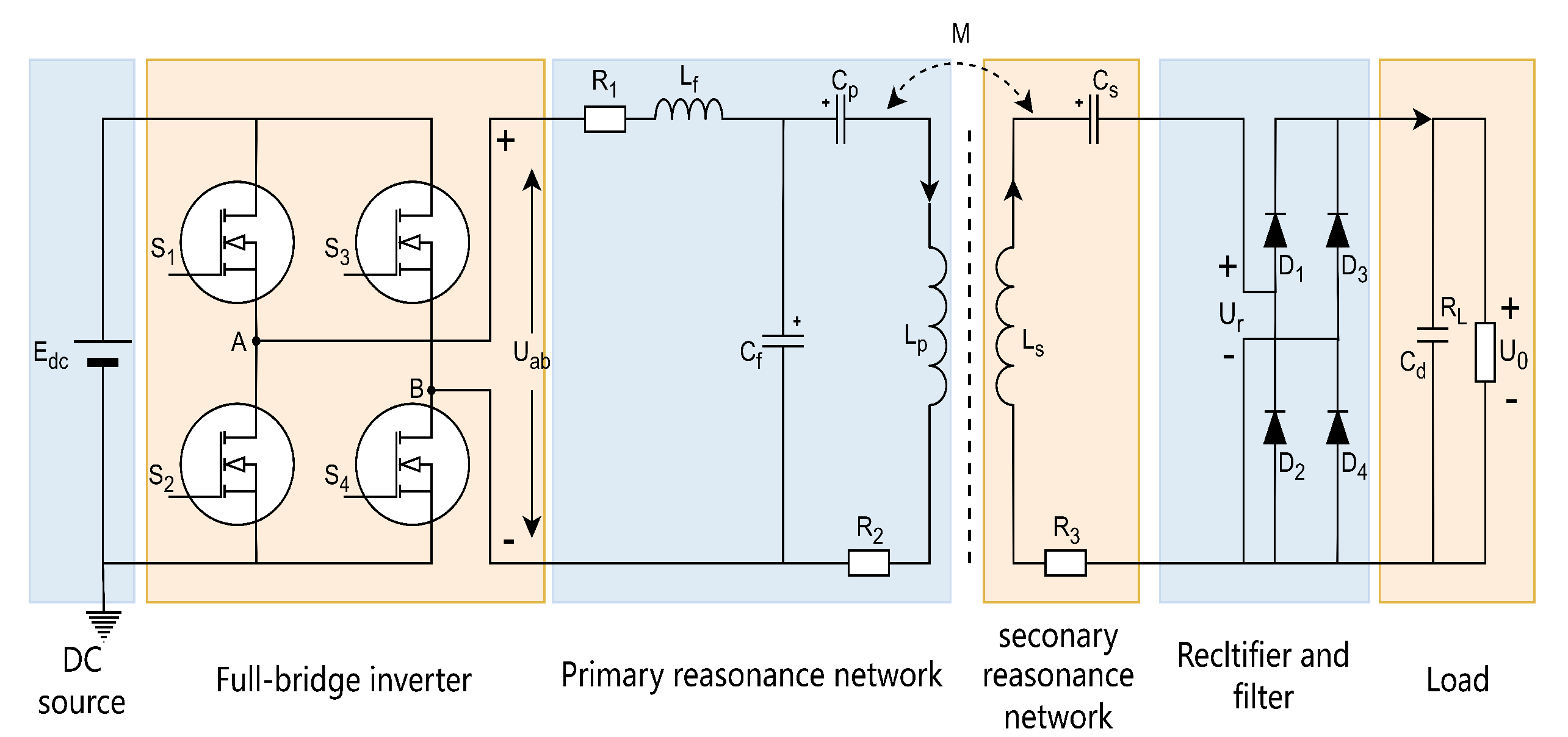
The LCC–S WPT topology investigated in this study is depicted in Figure 1. It comprises two main sections: a power-transmitter stage and a power-receiver stage.

The power transmitter stage comprises a DC source, a full-bridge inverter, a primary-side compensation network, and a transmitting coil [29,30,31]. The power receiver stage consists of a receiving coil, a secondary-side compensation network, a rectifier circuit, a filter network, and a load. The full-bridge inverter incorporates four controllable switches $S_1$–$S_4$. The alternating current output voltage $U_{ab}$ is regulated by adjusting the phase-shift angle between the driving signals of two adjacent switching legs. The primary-side compensation network employs an LCC composite compensation method, and the secondary-side compensation network adopts the S series compensation method, enabling the system to have the characteristics of constant voltage input and constant voltage output. The resistances of the compensating inductor $L_f$, the transmitter coil $L_p$, and the receiver coil $L_s$ are denoted by $R_1$, $R_2$, and $R_3$, respectively. The mutual inductance between the transmitter and receiver coils is denoted by M. The rectifier circuit comprises four diodes ($D_1$–$D_4$), that rectify the AC input voltage into a DC voltage. A filter capacitor is then used to attenuate the ripple in the rectified voltage before it is supplied to the load resistance $R_L$. The voltage across $R_L$, denoted $U_0$, is the system output. The remainder of this section details and analyzes the modeling procedure.

2.2. State Estimation from Input–Output Data

The WPT system is represented by the following form:

$$\left\{\begin{array}{c}x(k+1)=A_{\mathrm{t}}x\left(k\right)+B_{\mathrm{t}}u\left(k\right),\hfill \\ y\left(k\right)=C_{\mathrm{t}}x\left(k\right)+z\left(k\right)\hfill \end{array}\right.$$

(1)

where input $u\left(k\right)\in {\mathbb{R}}^m$, state $x\left(k\right)\in {\mathbb{R}}^n$, output $y\left(k\right)\in {\mathbb{R}}^p$ and measurement noise $z\left(k\right)\in {\mathbb{R}}^p$. Throughout this paper, it is assumed that the true state-space matrices ($A_{true}$, $B_{true}$, $C_{true}$) and the noise are unknown. Only the input–output measurements from the real system are available.

$$\begin{array}{cc}\hfill & u\left(0\right),u\left(1\right),\dots ,u(k-1),\hfill \\ & y\left(0\right),y\left(1\right),\dots ,y(k-1).\hfill \end{array}$$

The data are assembled into the following matrices

$$\begin{array}{cc}\hfill & U_k:=\left[\begin{array}{cccc}u\left(0\right)\hfill & u\left(1\right)\hfill & \dots \hfill & u\left(k\right)\hfill \end{array}\right],\hfill \\ \hfill & Y_k:=\left[\begin{array}{cccc}y\left(0\right)\hfill & y\left(1\right)\hfill & \dots \hfill & y\left(k\right)\hfill \end{array}\right].\hfill \end{array}$$

We can estimate the state $x\left(k\right)$ and construct the state matrix from the measured input and output data

$$\begin{array}{cc}\hfill & X_k:=\left[\begin{array}{cccc}x\left(0\right)\hfill & x\left(1\right)\hfill & \dots \hfill & x\left(k\right)\hfill \end{array}\right],\hfill \\ \hfill & X_{k_{+}}:=\left[\begin{array}{cccc}x\left(1\right)\hfill & x\left(2\right)\hfill & \dots \hfill & x\left(k\right)\hfill \end{array}\right].\hfill \end{array}$$

From (1), the system’s impulse-response sequence is expressed as follows:

$$G_t=\left\{\begin{array}{cc}0,\hfill & t=0\hfill \\ C{A}^{t-1}B,\hfill & t=1,2,\dots \hfill \end{array}\right.$$

Under persistent excitation, the following holds:

$$\begin{array}{c}\left[y\right(0) y(1) \dots y(k-1\left)\right]\\ \begin{array}{c}\\ \hfill & =\left[G_{t-1}\dots G_0\right]\left[\begin{array}{ccccc}0& \dots & u\left(0\right)& \dots & u(k-t)\\ ⋮& \ddots & u\left(1\right)& \dots & u(k-t+1)\\ 0& ⋮& ⋮& & ⋮\\ u\left(0\right)& \dots & u(t-1)& \dots & u(k-1)\end{array}\right]\hfill \end{array}\end{array}$$

(2)

Next, we introduce some notation. Let

$$\begin{array}{cc}\hfill {\mathcal{l}}_{\mathrm{t}}& :={\left[\begin{array}{cccc}{C}^{\top }\hfill & A^{\top }{C}^{\top }\hfill & \dots \hfill & {\left(A^{k-1}\right)}^{\top }{C}^{\top }\hfill \end{array}\right]}^{\top },\hfill \\ \hfill & {\xi }_{\mathrm{t}}:=\left[\begin{array}{cccc}B\hfill & AB\hfill & \dots \hfill & A^{k-1}B\hfill \end{array}\right].\hfill \end{array}$$

(3)

$$H={\mathcal{l}}_{\mathrm{k}}{\xi }_{\mathrm{k}}=\left[\begin{array}{ccccc}{G}_1& G_2& \dots & \dots & G_t\\ G_2& G_3& \dots & \dots & G_{t+1}\\ \dots & \dots & \dots & \dots & \dots \\ G_t& G_{t+1}& \dots & \dots & G_{2t-1}\end{array}\right].$$

(4)

Through the singular value decomposition of H [32], we obtain

$$H=\left(U{{\mathrm{\Sigma }}_{\mathrm{svd}}}^{{\displaystyle \frac{1}{2}}}\right)\left({{\mathrm{\Sigma }}_{\mathrm{svd}}}^{{\displaystyle \frac{1}{2}}}{V}^{\top }\right)=\left(U{{\mathrm{\Sigma }}_{\mathrm{svd}}}^{{\displaystyle \frac{1}{2}}}\right)T{T}^{-1}\left({{\mathrm{\Sigma }}_{\mathrm{svd}}}^{{\displaystyle \frac{1}{2}}}{V}^{\top }\right)$$

(5)

where ${\mathcal{l}}_{\mathrm{k}}=U{{\mathrm{\Sigma }}_{\mathrm{svd}}}^{{\displaystyle \frac{1}{2}}}$, ${\xi }_{\mathrm{k}}={{\mathrm{\Sigma }}_{\mathrm{svd}}}^{{\displaystyle \frac{1}{2}}}{V}^{\top }$ and T is an arbitrary nonsingular matrix (which can be chosen as the identity matrix I). The matrix ${\mathcal{l}}_{\mathrm{k}}$ is given by the definition of H and its singular value decomposition.

Let

$${\mathrm{\Phi }}_{\mathrm{t}}=\left[\begin{array}{ccccc}0& 0& \dots & \dots & 0\\ CB& 0& 0& \dots & 0\\ \dots & \dots & \dots & \dots & ⋮\\ C{A}^{t-2}B& C{A}^{t-3}B& \dots & \dots & 0\end{array}\right]$$

(6)

Then, we can get

$$\begin{array}{cc}\hfill & {\mathcal{l}}_t[x\left(0\right)...x\left(t\right)]\hfill \\ \hfill & =[I-{\mathrm{\Phi }}_t]\left[\begin{array}{ccc}y\left(0\right)& \dots & y\left(t\right)\\ ⋮& ⋮& ⋮\\ y\left(t\right)& \dots & y\left(2t\right)\\ u\left(0\right)& \dots & u\left(t\right)\\ ⋮& ⋮& ⋮\\ u\left(t\right)& ...& u\left(2t\right)\end{array}\right].\hfill \end{array}$$

(7)

Under the assumption of observability, ${\mathcal{l}}_t$ ($t>n$) is full column rank, which implies ${\mathcal{l}}_t^{†}{\mathcal{l}}_t=I_n$. Then we can apply ${\mathcal{l}}_t^{†}$ to (7), express $x\left(t\right)$ through input and output data.

2.3. Data-Driven Petrov-Galerkin Projection

This work characterizes the noise model through a QMI formulation:

$$\mathcal{Z}:=\left\{Z\in {\mathbb{R}}^{(n+l)\times k}:{\left[\begin{array}{c}I\\ Z^T\end{array}\right]}^T\left[\begin{array}{cc}{\mathrm{\Psi }}_{11}\hfill & {\mathrm{\Psi }}_{12}\hfill \\ {\mathrm{\Psi }}_{12}^T\hfill & {\mathrm{\Psi }}_{22}\hfill \end{array}\right]\left[\begin{array}{c}I\\ Z^T\end{array}\right]\ge \mathbf{0}\right\},$$

(8)

where ${\mathrm{\Psi }}_{11}={\mathrm{\Psi }}_{11}^T\in {\mathbb{R}}^{(n+l)\times (n+l)}$, ${\mathrm{\Psi }}_{12}\in {\mathbb{R}}^{(n+l)\times k}$, and ${\mathrm{\Psi }}_{22}={\mathrm{\Psi }}_{22}^{\top }\in {\mathbb{R}}^{k\times k}$. For a bounded and non-empty noise model, the matrices ${\mathrm{\Psi }}_{11}$, ${\mathrm{\Psi }}_{12}$, and ${\mathrm{\Psi }}_{22}$ satisfy ${\mathrm{\Psi }}_{22}<0$ and ${\mathrm{\Psi }}_{11}-{\mathrm{\Psi }}_{12}{\mathrm{\Psi }}_{22}^{-1}{\mathrm{\Psi }}_{12}^{\top }>0$.

Let us define the collection of systems that reconcile with the measured data as follows:

$$\mathrm{\Sigma }:=\left\{\left(\begin{array}{c}A,B,C\end{array}\right):\left[\begin{array}{c}{X}_{+}\\ Y_{-}\end{array}\right]-\left[\begin{array}{cc}A& B\\ C& 0\end{array}\right]\left[\begin{array}{c}{X}_{-}\\ U_{-}\end{array}\right]\in \mathcal{Z}\right\},$$

(9)

where $\mathcal{Z}\in {\mathbb{R}}^{(n+p)\times k}$ is the noise term

$$(A_t,B_t,C_t)\in \mathrm{\Sigma }.$$

(10)

Based on the definitions of $\mathrm{\Sigma }$ and (8), $(A,B,C)$ belongs to $\mathrm{\Sigma }$ precisely when the following QMI holds

$${\left[\begin{array}{cc}I& 0\\ 0& I\\ A^{\top }& C^{\top }\\ B^{\top }& 0\end{array}\right]}^{\top }\mathbf{N}\left[\begin{array}{cc}I& 0\\ 0& I\\ A^{\top }& C^{\top }\\ B^{\top }& 0\end{array}\right]\ge 0,$$

(11)

where

$$\mathbf{N}:=\left[\begin{array}{ccc}I& 0& X_{k_{+}}\\ 0& I& Y_{k-1}\\ 0& 0& -X_{k-1}\\ 0& 0& -U_{k-1}\end{array}\right]\left[\begin{array}{cc}{\mathrm{\Psi }}_{11}& {\mathrm{\Psi }}_{12}\\ {\mathrm{\Psi }}_{12}^T& {\mathrm{\Psi }}_{22}\end{array}\right]{\left[\begin{array}{ccc}I& 0& X_{k_{+}}\\ 0& I& Y_{k-1}\\ 0& 0& -X_{k-1}\\ 0& 0& -U_{k-1}\end{array}\right]}^{\top }.$$

(12)

In characterizing the set of systems that explain the data, one may wonder whether the set $\mathrm{\Sigma }$ is bounded and has a nonempty interior. The following proposition provides a necessary and sufficient condition for these properties, which depends solely on the data.

Lemma 1

([33]). Under the condition of continuous excitation of the system, the set Σ is bounded and has a nonempty interior if and only if there exists a matrix $S\in {\mathbb{R}}^{(n+m)\times (n+l)}$ satisfying

$${\left[\begin{array}{c}I\\ S\end{array}\right]}^{\top }N\left[\begin{array}{c}I\\ S\end{array}\right]>0.$$

(13)

This study does not aim to identify the true system in (1); instead, it seeks to derive a reduced-order approximation directly from the available data.

As a first step, consider matrices $\tilde{W},\tilde{V}\in {\mathbb{R}}^{n\times r}$, that satisfy ${\tilde{W}}^{\top }\tilde{V}=I$ and $r<n$. Employing Petrov-Galerkin projection, we define the reduced-order system $\tilde{\mathrm{\Sigma }}$ as

$$\tilde{\mathrm{\Sigma }}:=\left({\tilde{W}}^{\top }A\tilde{V},{\tilde{W}}^{\top }B,C\tilde{V}\right).$$

where $(A,B,C)\in \mathbf{\Sigma }$.

Lemma 2

([33]). Consider the set Σ. Under persistent excitation, assume there exists a matrix S satisfying (13). Let $\tilde{W},\tilde{V}\in {\mathbb{R}}^{n\times r}$ be such that ${\tilde{W}}^{\top }\tilde{V}=I$ and $r<n$. Then, the set $\tilde{\mathrm{\Sigma }}$ of reduced-order models of Σ using matrices $\tilde{W},\tilde{V}$ satisfies

$$\tilde{\mathrm{\Sigma }}=\left\{(\tilde{A},\tilde{B},\tilde{C}):{\left[\begin{array}{cc}I& 0\\ 0& I\\ {\tilde{A}}^{\top }& {\tilde{C}}^{\top }\\ {\tilde{B}}^{\top }& 0\end{array}\right]}^{\top }{N}_{vw}\left[\begin{array}{cc}I& 0\\ 0& I\\ {\tilde{A}}^{\top }& {\tilde{C}}^{\top }\\ {\tilde{B}}^{\top }& 0\end{array}\right]\ge 0\right\},$$

where

$$N_{vw}:=\left[\begin{array}{cc}{W}^{\top }\left(N\mid N_{22}+N_{12}{N}_{22}^{-1}V{\left(V^{\top }{N}_{22}^{-1}V\right)}^{-1}{V}^{\top }{N}_{22}^{-1}{N}_{12}^{\top }\right)W& W^{\top }{N}_{12}{N}_{22}^{-1}V{\left(V^{\top }{N}_{22}^{-1}V\right)}^{-1}\\ {\left(V^{\top }{N}_{22}^{-1}V\right)}^{-1}{V}^{\top }{N}_{22}^{-1}{N}_{12}^{\top }W& {\left(V^{\top }{N}_{22}^{-1}V\right)}^{-1}\end{array}\right]$$

(14)

and

$$W:=\left[\begin{array}{cc}\tilde{W}& \\ & I_p\end{array}\right],V:=\left[\begin{array}{cc}\tilde{V}& \\ & I_m\end{array}\right].$$

Lemma 2 offers a clear data-reduction interpretation: the matrix $\tilde{\mathrm{\Sigma }}$, which encompasses all reduced-order models, is determined solely by the projection matrices $\tilde{V}$ and $\tilde{W}$ together with the original data matrix N.

This section presents reduced-order system approximations consistent with the collected data, assuming prescribed projection matrices $\tilde{W}$ and $\tilde{V}$. Thus far, no restrictions have been imposed on these matrices; hence, Lemma 2 holds for any Petrov–Galerkin projection. The subsequent section constructs a data-driven Petrov–Galerkin projection based on a generalized balancing framework.

2.4. Data-Driven Generalized Balanced Truncation

Lyapunov balanced truncation is a classical reduction technique; this section proposes a data-driven approach based on a novel GLB framework to derive reduced-order models.

For the discrete-time system (1), let $P,Q\in {\mathbb{R}}^{n\times n}$ be symmetric positive definite. If P satisfies

$$AP{A}^{\top }-P+B{B}^{\top }<0,$$

(15)

it is called the generalized controllability Gramian; if Q satisfies

$$A^{\top }QA-Q+C^{\top }C<0,$$

(16)

it is called the generalized observability Gramian. This represents a strict generalization of the standard Gramian definitions presented in [34]. Specifically, the generalized controllability and observability Gramians satisfy the inequality bounds $P>P_0$ and $Q>Q_0$, where $Q_0$ and $P_0$ solve the standard Lyapunov equations. It is worth stressing that such generalized Gramians exist only when the system $\mathrm{\Sigma }$ is asymptotically stable, i.e., $\rho \left(A\right)<1$, with $\rho (·)$ denoting the spectral radius.

Remark 1.

As shown in ([35] Ch. 7), the satisfaction of either (15) or (16) guarantees that all systems in Σ are asymptotically stable.

The generalized Gramians facilitate the construction of a balanced realization of (1) in which they coincide and become diagonal. By Lemma 7.3 of [33], there exists a nonsingular matrix T such that

$$TP{T}^{\mathrm{T}}=T^{-\mathrm{T}}Q{T}^{-1}={\mathrm{\Sigma }}_H,$$

where ${\mathrm{\Sigma }}_H$ denotes the block-diagonal matrix of generalized Hankel singular values corresponding to Σ in (1), namely

$${\mathrm{\Sigma }}_H;=blkdiag\left({\mathrm{\lambda }}_1{I}_{h_1},{\mathrm{\lambda }}_2{I}_{h_2},\dots ,{\mathrm{\lambda }}_k{I}_{h_k}\right),$$

(17)

where ${\mathrm{\lambda }}_1>{\mathrm{\lambda }}_2>\dots >{\mathrm{\lambda }}_k>0$. The integer $h_i$ is the multiplicity of ${\mathrm{\lambda }}_i$ for $i=1,\dots ,k$, and the dimensions satisfy ${\sum }_{i=1}^k{h}_i=n$. Thus, the realization is termed GLB. Specifically, the balanced form realization is given by the transformed matrices:

$$A_b:=TA{T}^{-1},B_b:=TB,C_b:=C{T}^{-1}.$$

(18)

Finally, a reduced-order model is obtained via balanced truncation of the balanced system $(A_b,B_b,C_b)$. In fact, balanced truncation can be viewed as a Petrov–Galerkin projection method. Define the selection matrix $\mathrm{\Gamma }\in {\mathbb{R}}^{n\times r}$ by

$$\mathrm{\Gamma }:=\left[\begin{array}{c}{I}_r\\ 0\end{array}\right].$$

Setting

$$\tilde{V}=T^{-1}\mathrm{\Gamma },\tilde{W}=T^{\mathrm{T}}\mathrm{\Gamma },$$

and ${\tilde{W}}^{\mathrm{T}}\tilde{V}=I$. Therefore, applying the Petrov–Galerkin projection yields a reduced-order model of dimension r that is equivalent to the model obtained by balanced truncation.

Generalized balanced truncation guarantees retention of the original system’s key properties. Crucially, the system’s asymptotic stability remains intact.

Lemma 3

([33]). Assume that there exists a matrix S satisfying (13); define

$$N_p:={\left[\begin{array}{cc}{I}_n& 0\\ 0& 0\\ 0& I_{n+m}\end{array}\right]}^{\top }N\left[\begin{array}{cc}{I}_n& 0\\ 0& 0\\ 0& I_{n+m}\end{array}\right],$$

and

$$N_q:={\left[\begin{array}{ccc}{I}_n& 0& 0\\ 0& 0& 0\\ 0& 0& I_{n+l}\end{array}\right]}^{\top }{N}^{\star }\left[\begin{array}{ccc}{I}_n& 0& 0\\ 0& 0& 0\\ 0& 0& I_{n+l}\end{array}\right],$$

where

$$N^{\star }:=\left[\begin{array}{cc}0& -I_{n+m}\\ I_{n+l}& 0\end{array}\right]N^{-1}\left[\begin{array}{cc}0& -I_{n+l}\\ I_{n+m}& 0\end{array}\right].$$

Then, the system is asymptotically stable under continuous excitation, if and only if:

(i) There exist a symmetric positive-definite matrix P and a scalar $\alpha >0$ satisfying

$$\left[\begin{array}{ccc}P& 0& 0\\ 0& -P& 0\\ 0& 0& -I_m\end{array}\right]>\alpha N_p,$$

(19)

(ii) There exist a symmetric positive-definite matrix Q and a scalar $\gamma >0$ satisfying

$$\left[\begin{array}{ccc}Q& 0& 0\\ 0& -Q& 0\\ 0& 0& -I_l\end{array}\right]>\gamma N_q.$$

(20)

For each system $(A,B,C)\in \mathrm{\Sigma }$, a balanced realization can be constructed using (18). These balanced realizations are then used to derive reduced-order models directly from the data.

Under the Petrov–Galerkin projection, generalized balanced truncation maps each system in $\mathrm{\Sigma }$ onto a reduced-order representation, with the entire family of such models residing in the set

$$\tilde{\mathrm{\Sigma }}:=\left\{({\tilde{W}}^{\top }A\tilde{V},{\tilde{W}}^{\top }B,C\tilde{V})\right\}.$$

Accordingly, $\tilde{\mathrm{\Sigma }}$ denotes the set of all reduced-order models obtained by the generalized balanced-truncation technique. The reduced matrix $N_{vw}$ is completely determined by the data matrix N and the projection matrices $\tilde{V}=T^{-1}\mathrm{\Gamma }$ and $\tilde{W}=T^{\top }\mathrm{\Gamma }$. These projection matrices are directly constructed from the collected data, as described in Lemma 3.

By definition, every triplet $(\tilde{A},\tilde{B},\tilde{C})\in \tilde{\mathrm{\Sigma }}$ is obtained by applying generalized balanced truncation to a system in $\mathrm{\Sigma }$. Hence, its spectral radius satisfies $\rho \left(\tilde{A}\right)<1$, and the resulting reduced-order system is asymptotically stable. Thus far, we have shown how to compute a set of reduced-order models directly from the given input-output data, all of which are guaranteed to be asymptotically stable. Following the method in [36], a specific pair $(\tilde{A},\tilde{B})$ can be selected from $\tilde{\mathrm{\Sigma }}$ using the expression

$$\begin{array}{cc}\hfill \left[\begin{array}{c}\tilde{A} \tilde{B}\end{array}\right]& =-{\tilde{N}}_{12}{\tilde{N}}_{22}^{-1}+{\left(N_{vw}\mid {\tilde{N}}_{22}\right)}^{{\displaystyle \frac{1}{2}}}\mathrm{\Phi }{\left({(-{\tilde{N}}_{22})}^{-1}\right)}^{{\displaystyle \frac{1}{2}}},\hfill \\ \hfill \tilde{C}& ={\mathcal{l}}_{\mathrm{t}}\tilde{V}\hfill \end{array}$$

(21)

for some uncertain $\mathrm{\Phi }\in {\mathbb{R}}^{(n+p)\times (n+m)}$ with ${\mathrm{\Phi }}^{\top }\mathrm{\Phi }<I$, where the partition

$$N_{vw}=\left[\begin{array}{cc}{\tilde{N}}_{11}& {\tilde{N}}_{12}\\ {\tilde{N}}_{12}^{\top }& {\tilde{N}}_{22}\end{array}\right],$$

was used with ${\tilde{N}}_{11}\in {\mathbb{R}}^{r\times r}$ and ${\tilde{N}}_{22}\in {\mathbb{R}}^{(r+m)\times (r+m)}$.

In summary, Algorithm 1 provides a data-driven generalized lyapunov balanced truncation approach. The resulting reduced-order model is given by the following state-space equations:

$$\left\{\begin{array}{c}\mathrm{x}(k+1)=\tilde{A}x\left(k\right)+\tilde{B}u\left(k\right),\hfill \\ y\left(k\right)=\tilde{C}x\left(k\right).\hfill \end{array}\right.$$

(22)

Remark 2.

In contrast to traditional model order reduction techniques such as Moment Matching or Mode Selection, the generalized Lyapunov balanced truncation method proposed herein ensures a principled retention of the dominant state-energy components. This approach not only guarantees stability preservation but also yields a low-order model with clear physical interpretability and a user-specified order. These properties make it particularly applicable to the analysis and control of power electronic systems [32,37].

Algorithm 1: Data-Driven Generalized Lyapunov Balanced Truncation
Input:	Input, state, output data $(U_k,X_k,Y_k)$, noise model $\mathcal{Z}$ and target
	reduced-order model dimension r.
Output:	Reduced-order model matrices: $\tilde{A},\tilde{B},\tilde{C}$.
1.	Construct data matrices $N,N_p,N_q$.
2.	If the system is under conditions of continuous excitation, LMIs (19)
	and (20) possess feasible solutions then
	Evaluate P and Q
3.	Compute the transformation matrix T and the set ${\mathrm{\Sigma }}_H$ through direct
	computation based on the system Gramians P and Q.
4.	Construct projection matrices $\tilde{V}=T^{-1}\mathrm{\Gamma }$ and $\tilde{W}=T^{\top }\mathrm{\Gamma }$, where $\mathrm{\Gamma }=\left[\begin{array}{c}{I}_r\\ 0\end{array}\right]$.
	Compute the data matrix $N_{vw}$ using (14).
5.	Compute the reduced-order model parameters using (21).
6.	Return $\tilde{A},\tilde{B},\tilde{C}$.

3. Controller Design

For WPT systems, maintaining a stable output is a crucial control objective.To this end, we utilize the data-driven ROM (22) as a foundation for controller design. Specifically, a Linear-Quadratic Regulator (LQR) framework is adopted to synthesize a PI controller, aimed at improving the system’s robustness and power transfer efficiency.

The LQR-PI controller is a conventional control strategy. It is designed by introducing an integral state variable $x_i\left(k\right)$, defined $x_i(k+1)=x_i\left(k\right)+e\left(k\right)$ with initial condition $x_i\left(0\right)=0$. The control law is given by

$$u\left(k\right)=K_{p}e\left(k\right)+K_{i}x\left(k\right)$$

(23)

where $u\left(k\right)$ is the controller output, $e\left(k\right)=r\left(k\right)-y\left(k\right)$ is the tracking error, and $K_p$, $K_i$ are the proportional and integral gains, respectively. The control design objective is to select these gains to ensure closed-loop stability.

To transform the PI control problem into the LQR framework, an augmented state vector is constructed

$$\overline{x}:=\left[\begin{array}{c}x\left(k\right)\\ x_i\left(k\right)\end{array}\right].$$

The state-space model for the augmented system is given by:

$$x(k+1)=\overline{A}\overline{x}\left(k\right)+\overline{B}u\left(k\right)+{\overline{B}}_{r}r\left(k\right)$$

(24)

where

$$\overline{A}=\left[\begin{array}{cc}\tilde{A}& 0\\ -\tilde{C}& I\end{array}\right],\overline{B}=\left[\begin{array}{c}\tilde{B}\\ 0\end{array}\right],{\overline{B}}_r=\left[\begin{array}{cc}0& I\end{array}\right].$$

Define the quadratic performance index:

$$J=\sum _{k=0}^{\infty }\left[e^{\top }\left(k\right)Q_{e}e\left(k\right)+{\overline{x}}_i^{\top }\left(k\right)Q_i{\overline{x}}_i\left(k\right)+u^{\top }\left(k\right)Ru\left(k\right)\right]$$

(25)

The performance index J depends on the tracking error $e\left(k\right)=r\left(k\right)-y\left(k\right)$. However, for state-feedback control design, the reference $r\left(k\right)$ does not affect the optimization of the control law. The cost function can therefore be simplified to the standard LQR form:

$$J=\sum _{k=0}^{\infty }{\overline{x}}^{\top }\left(k\right)\overline{Q}\overline{x}\left(k\right)+u^{\top }\left(k\right)Ru\left(k\right)$$

(26)

where $\overline{Q}=\left[\begin{array}{cc}{C}^{\top }{Q}_{e}C& 0\\ 0& Q_i\end{array}\right]$.

By solving the discrete-time algebraic Riccati equation:

$$P={\overline{A}}^{\top }P\overline{A}-{\overline{A}}^{\top }P\overline{B}{({\overline{B}}^{\top }P\overline{B}+R)}^{-1}{\overline{B}}^{\top }P\overline{A}+\overline{Q}.$$

The optimal feedback gain matrix for the augmented system is given by:

$$K=-{({\overline{B}}^{\top }P\overline{B}+R)}^{-1}{\overline{B}}^{\top }P\overline{A}.$$

This gain matrix inherently contains the PI controller structure:

$$K=\left[\begin{array}{cc}-K_p\tilde{C}& K_i\end{array}\right].$$

The parameters of the PI controller can be directly extracted from this matrix.

Remark 3.

In contrast to conventional controller design approaches—which rely on detailed circuit models or explicit mutual inductance formulations—the fully data-driven framework proposed in this paper integrates system identification and control synthesis into a unified procedure using solely input–output data. This methodology significantly reduces dependency on precise physical parameters and demonstrates enhanced adaptability and synergistic integration of modeling and control, as validated experimentally [38,39].

4. Experimental Results

4.1. Experimental Prototype Implementation

To experimentally validate the efficacy of the proposed data-driven model reduction technique and the corresponding PI control strategy, an LCC–S wireless WPT system platform was constructed for testing.

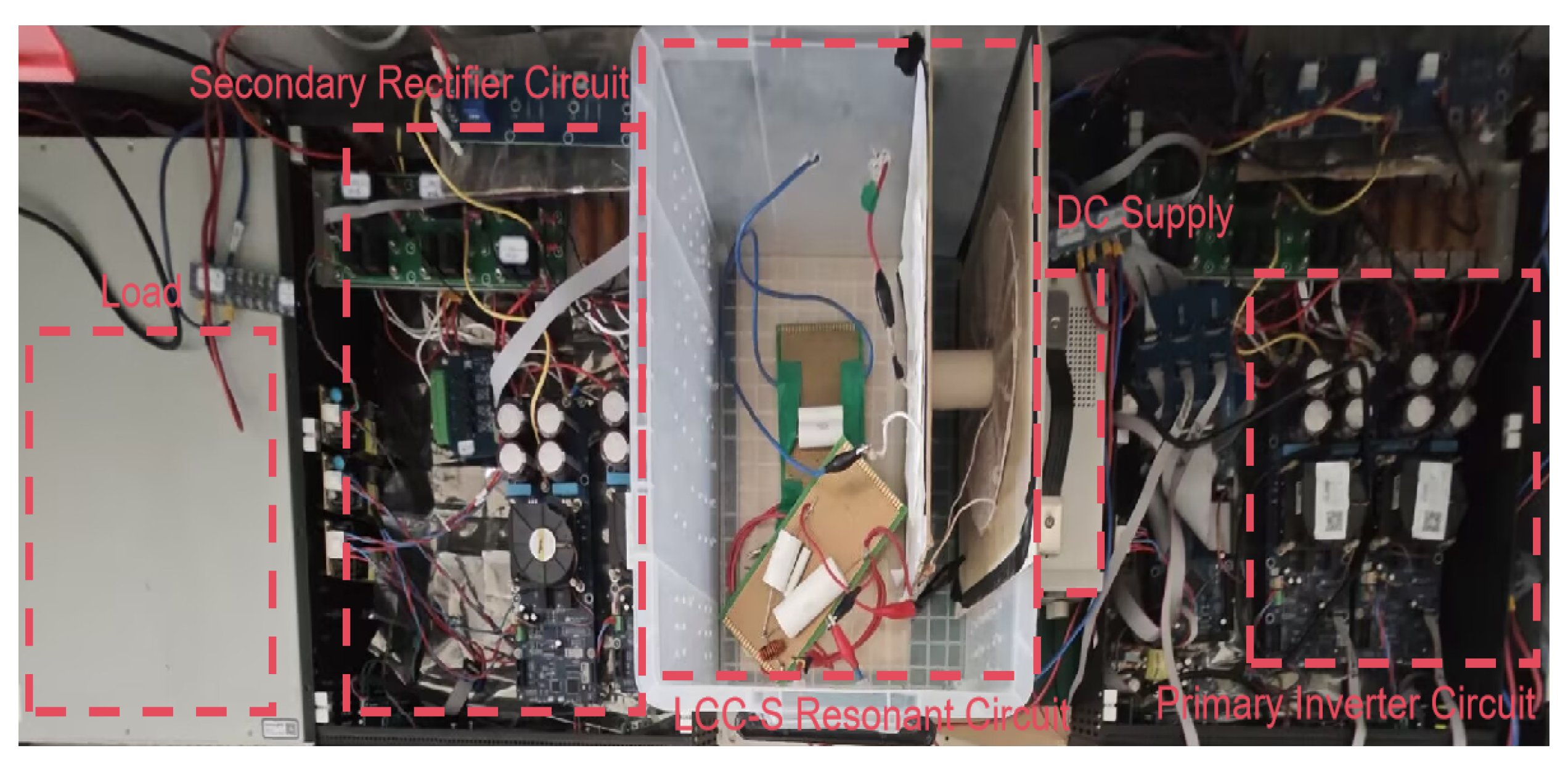
The system topology is illustrated in Figure 1. A digital signal processor samples the input and output voltages using its integrated analog-to-digital converter and communicates these measurements to a host PC via a serial interface. The PC performs system identification using Algorithm 1 and subsequently designs the controller in an offline manner. A photograph of the implemented LCC–S resonant WPT prototype is shown in Figure 2. The experimental setup includes a DC power supply, a full-bridge inverter, an LCC–S compensation network, a rectifier circuit, and a resistive load. Key design specifications and implementation details of the prototype are summarized as follows:

(1) The inverter power stage is implemented using four SiC MOSFETs (NTHL020 N120SC1) in a full-bridge configuration, supplied by an adjustable DC source (LPS605D). A TMS320F28335 DSP on an integrated controller board generates the drive and control signals, while simultaneously measuring the input and output voltages of the system under test. The acquired voltage data are transmitted to a host PC via a serial interface for subsequent execution of data-driven modeling and model reduction algorithms.

(2) The prototype incorporates circular resonant coils with a 7 cm air gap. Each coil is wound with 29 turns of Litz wire, featuring an inner diameter of 4 cm and an outer diameter of 11 cm.

(3) For the LCC–S compensation network, metallized polypropylene film capacitors are used: two series capacitors, $C_p=35$ nF and $C_s=28$ nF, along with a parallel capacitor $C_f=150$ nF.

(4) The device parameters reported in

Table 1. Key specifications of the prototype.

Element	Parameter	Value
Inverter switching frequency	${\mathrm{f}}_s$	85 kHz
Primary parallel compensating inductor	${\mathrm{L}}_f$	23 $\mathsf{\mu }\mathrm{H}$
Primary inductance	${\mathrm{L}}_p$	121.98 $\mathsf{\mu }\mathrm{H}$
Secondary inductance	${\mathrm{L}}_s$	124.39 $\mathsf{\mu }\mathrm{H}$
Primary internal resistance	${\mathrm{R}}_p$	103.13 mΩ
Secondary internal resistance	${\mathrm{R}}_s$	108.22 mΩ
Primary parallel compensation capacitor	${\mathrm{C}}_f$	$150\mathrm{nF}$
Primary series compensation capacitance	${\mathrm{C}}_p$	$35\mathrm{nF}$
Secondary series compensation capacitance	${\mathrm{C}}_s$	$28\mathrm{nF}$
Mutual inductance	M	29.85 $\mathsf{\mu }\mathrm{H}$
Filtering inductor	${\mathrm{L}}_{fc}$	47 $\mathsf{\mu }\mathrm{H}$
Filtering capacitance	${\mathrm{C}}_{fc}$	470 $\mathsf{\mu }\mathrm{F}$
Load resistance	${\mathrm{R}}_L$	10 $\mathrm{\Omega }$
DC output voltage	${\mathrm{E}}_{dc}$	20 V

were obtained with a VICTOR4092E meter.

4.2. Validation of Data-Driven Modeling

The experimental procedure began with data acquisition, where input-output data sequences were transmitted to a host PC over a serial link for subsequent model construction. The system model was constructed using 1000 input-output data samples collected during the system’s operation. The sampling interval was set to $T_s=0.1\mathrm{ms}$, corresponding to a sampling frequency of 85 kHz, which satisfies the conditions of persistent excitation and observability. It is noteworthy that the collected data inherently contain measurement noise, which is systematically addressed in our data-driven modeling framework through the QMI formulation introduced in Section 2.2. Specifically, the noise parameters are determined by acquiring measurement data from the output channel under zero-input conditions. The calculated measured noise variance is $1.346\times {10}^{-4}$. To satisfy the mathematical constraints of boundedness and non-emptiness of the noise set and ensure the rigorous validity of the QMI defined set, a conservative treatment of the measured variance value is adopted. Accordingly, we set ${\mathrm{\Psi }}_{11}=1.35e^{-4}I$, ${\mathrm{\Psi }}_{12}=0$, and ${\mathrm{\Psi }}_{22}=-I$. This approach does not require explicit pre-filtering of the data; instead, it incorporates these noise bounds directly into the model construction process, ensuring that the resulting reduced-order models are robust to uncertainties and perturbations. Based on the collected data, the data matrices $U_k,Y_k,X_k$ were constructed, and the original system was modeled using the Petrov-Galerkin projection and the GLB method proposed in Section 2.

Existing studies have achieved the reduction of WPT systems to 2nd-order models using methods such as energy balancing and the extended describing function [14,40]; however, these approaches are often complex. To demonstrate that the data-driven method proposed in this paper offers greater simplicity while maintaining modeling accuracy, this section compares the resulting 2nd- to 4th-order models against an 11th-order high-fidelity reference model obtained via conventional system identification.

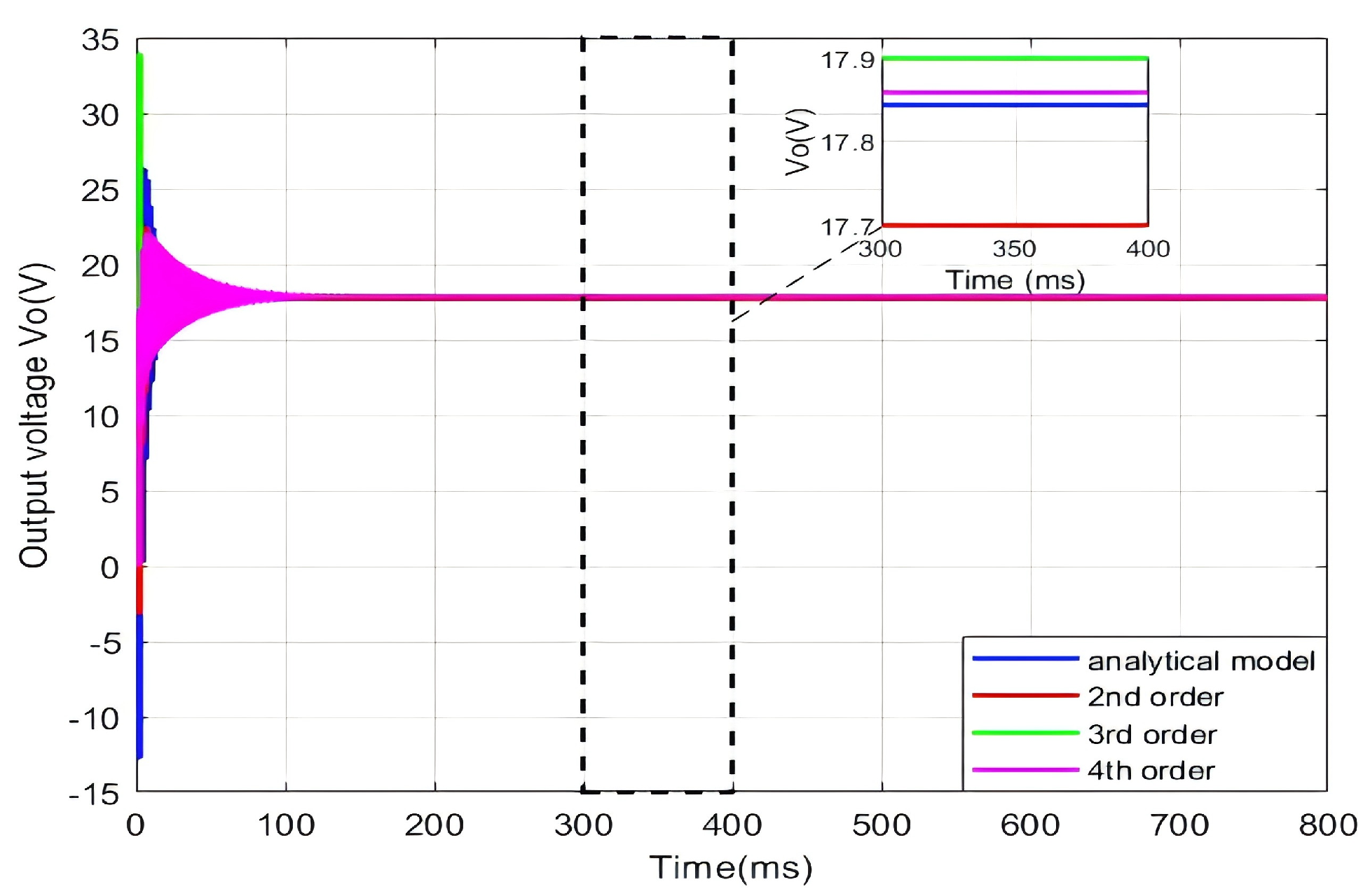
The comparison between the 2nd- to 4th-order reduced-order models constructed using the data-driven order reduction approach and the 11th-order reference model established via state-space identification is shown in Figure 3. The response curves indicate that the fourth-order model exhibits relatively small steady-state error; the third-order model, while showing slightly higher overshoot, still maintains favorable steady-state accuracy; and the second-order model demonstrates limited overshoot with marginally higher steady-state error compared to the former. Overall, the 2nd- to 4th-order reduced models perform similarly to the 11th-order reference model in terms of dynamic behavior, effectively capturing the dominant dynamic characteristics of the system.

4.3. Validation of the LQR–PI Controller

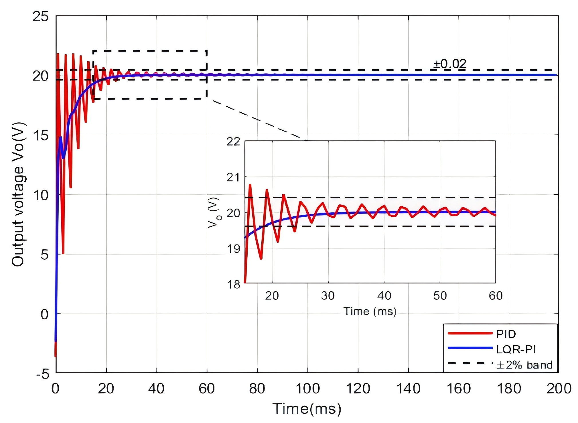
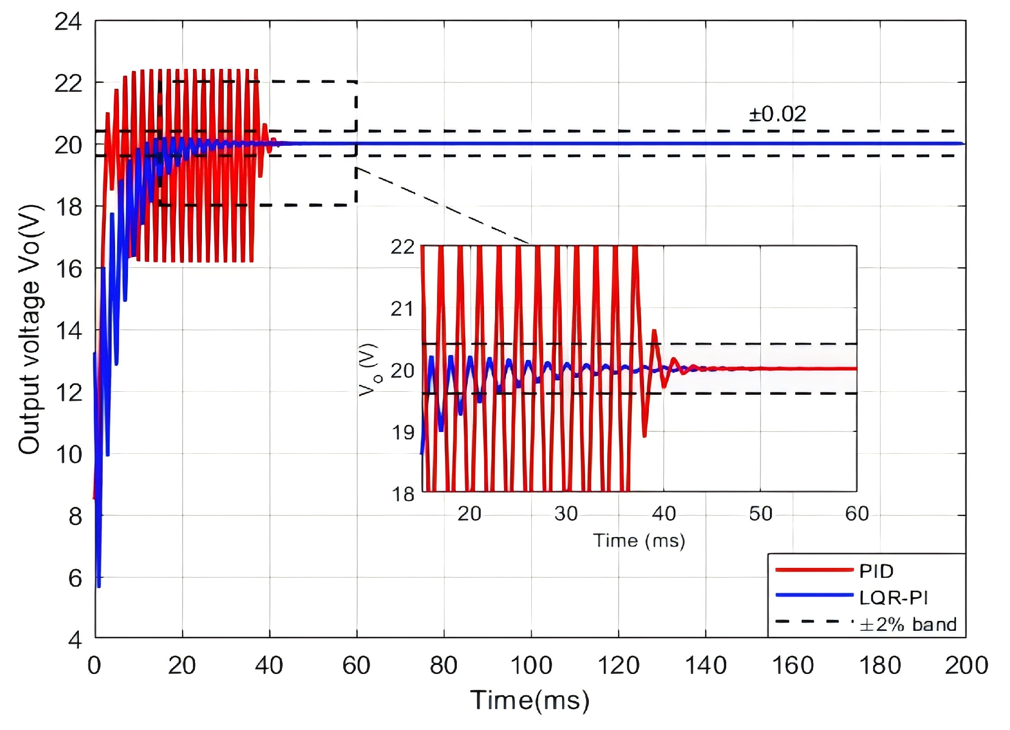
To assess the performance of the proposed control strategy under varying model complexities, system representations with different orders are utilized as control targets. A comparative evaluation is performed between a conventional PID controller and the proposed LQR-PI control scheme. The control objective is to regulate the output voltage to a reference of 20 V. The closed-loop performance is evaluated using 2nd- to 4th-order models. Figure 4, Figure 5 and Figure 6 present the output voltage responses achieved with the PID and LQR-PI controllers, respectively.

Figure 4 shows the response for the second-order system. The PID controller yields a 9% overshoot and a 24.2 ms settling time (within a 2% band). In contrast, the LQR-PI controller responds faster with almost no overshoot and settles in 19 ms. Under the third-order model (Figure 5), the system dynamics become more complex. The PID controller’s overshoot increases to 12%, and its settling time is 38.9 ms. The LQR-PI controller, while exhibiting a slower initial rise, maintains almost no overshoot and a shorter settling time of 22.9 ms.

The output response of the fourth-order system is presented in Figure 6. Under this higher-order dynamics, both controllers exhibit overshoot, yet with markedly different performance. The PID controller suffers from a considerable overshoot (>20%) and exhibits pronounced oscillations, resulting in a prolonged settling time. In contrast, the LQR-PI controller demonstrates superior robustness, with a significantly reduced overshoot (<5%), a smooth response, and a rapid settling time of approximately 30 ms.

To further quantify the control performance difference between the two controllers under different order systems, this paper extracts typical dynamic performance indicators, including overshoot, settling time and root mean square error(RMSE), based on the response curves shown in Figure 4, Figure 5 and Figure 6. Here, the settling time is defined as the duration required for the system output to initially enter and subsequently stay within a ±2% tolerance band around the reference value.

Table 2. Dynamic Performance Comparison of PID and LQR-PI Controllers under Different System Orders.

System	Controller	Overshoot (%)	Settling Time (ms)	RMSE (V)
2nd	PID	9	24.2	3.3
	LQR-PI	0	19	1.91
3rd	PID	12	38.9	4.65
	LQR-PI	0	22.9	3.13
4th	PID	23.9	84	5.93
	LQR-PI	3.5	27.9	2.95

lists the performance comparison between the PID controller and the LQR-PI controller under different order models. The results indicate that as the system order increases, both the overshoot and settling time of the PID controller rise significantly, demonstrating a clear deterioration in dynamic performance. In contrast, the LQR-PI controller maintains low overshoot and rapid settling across all system orders, further validating its superior stability and dynamic response characteristics in complex systems.

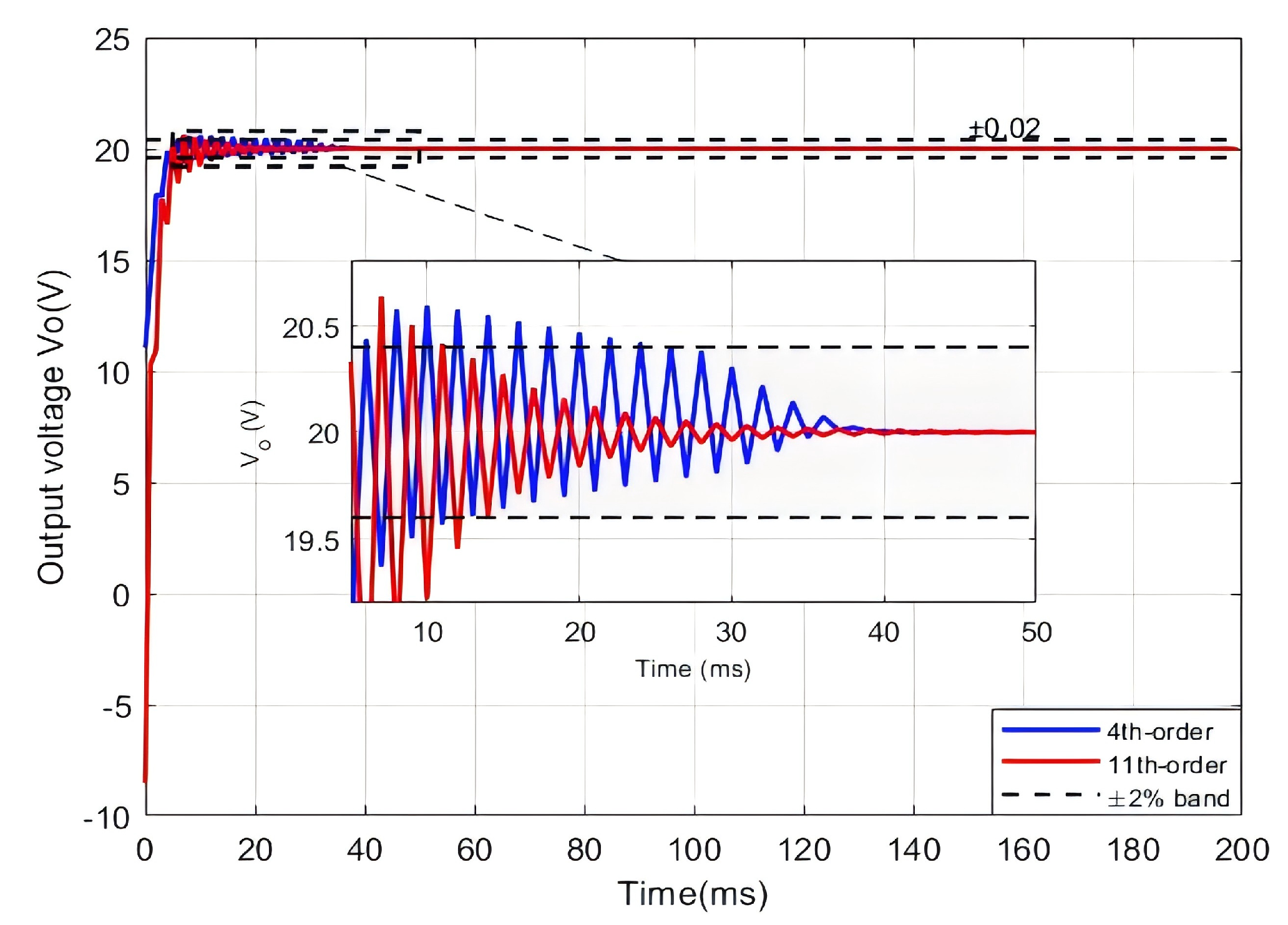
Next, we further compared the dynamic performance of the data-driven 4th-order model and the traditionally identified 11th-order model under LQR-PI control, as shown in Figure 7. It can be observed that the overall performance of both models is quite similar under LQR-PI control, with nearly identical overshoot. Although the 11th-order model enters the ±2% error band more quickly, it requires a longer time to reach the steady-state output compared to the 4th-order model. This result demonstrates that the proposed data-driven method not only simplifies the model but also effectively captures the system’s dominant dynamics with high fidelity. It proves that the controller’s performance is not compromised by the lower model order; conversely, by avoiding the inaccuracies and over-parameterization pitfalls of high-order physical identification, the data-driven approach provides a more robust and concise model for control design.

In summary, the experimental validation confirms the effectiveness of the proposed framework through the following aspects: First, the data-driven reduced-order model demonstrates dynamic behavior highly consistent with an 11th-order model derived from traditional identification. Second, the proposed LQR-PI control strategy consistently outperforms the conventional PID controller across models of various complexities. Furthermore, and more importantly, the controller based on the data-driven reduced-order model delivers performance on par with that based on the high-order traditional model. This conclusively establishes that the proposed data-driven method offers a superior pathway to high-performance control design for complex systems like WPT, achieving simplicity in modeling and control design without sacrificing accuracy and robustness.

5. Conclusions

This paper has presented a data-driven modeling and control method, providing a new approach for handling system uncertainties in industrial WPT applications, such as electric vehicle charging and power supply for medical equipment. This method has directly constructed a reduced-order state space model based on input-output data without relying on precise physical parameters. It has significantly reduced the model complexity while retaining the key dynamic characteristics of the system, and has designed a PI controller with integral behavior based on the LQR framework. Verification on the LCC-S type WPT experimental platform has shown that the obtained third-order and fourth-order reduction models are highly consistent with the behavior of the full-order system in terms of steady-state accuracy. This method has been particularly suitable for actual WPT systems with limited model information or frequent parameter changes, and has demonstrated strong engineering applicability. Future research will further expand this framework to nonlinear system modeling and multi-objective control strategies to promote its wide application in industrial WPT.