LF-Net: A Lightweight Architecture for State-of-Charge Estimation of Lithium-Ion Batteries by Decomposing Global Trend and Local Fluctuations

Abstract

Accurate estimation of the State of Charge (SOC) of lithium-ion batteries under complex operating conditions remains challenging, as the SOC signal combines a global linear (quasi-linear) trend with localized dynamic fluctuations driven by polarization, ion diffusion, temperature gradients, and load transients. In practice, open-circuit-voltage (OCV) approaches are affected by hysteresis and parameter drift, while high-fidelity electrochemical models require extensive parameterization and significant computational resources that hinder their real-time deployment in battery management systems (BMS). Purely data-driven methods capture temporal patterns but may under-represent abrupt local fluctuations and blur the distinction between trend and fluctuation, leading to biased SOC tracking when operating conditions change. To address these issues, LF-Net is proposed. The architecture decomposes battery time series into long-term trend and local fluctuation components. A linear branch models the quasi-linear SOC evolution. Multi-scale convolutional and differential branches enhance sensitivity to transient dynamics. An adaptive Fusion Module aggregates the representations, improving interpretability and stability, and keeps the parameter budget small for embedded hardware. Our experimental results demonstrate that the proposed model achieves a mean absolute error (MAE) of 0.0085 and a root-mean-square error (RMSE) of 0.0099 at 40 °C, surpassing mainstream models and confirming the method’s efficacy.

1. Introduction

1.1. Motivation

LiFePO₄ batteries have become a foundational component in electric vehicles (EVs) and stationary energy storage, driven by their safety profile, long cycle life, and cost-effectiveness [1,2]. Their adoption is further supported by the ability to maintain stable operation under a wide range of environmental and load conditions, which is essential for large-scale deployment in transportation and grid applications [3]. In these systems, SOC is a critical parameter for BMS, as it directly determines energy availability, operational safety, and the prevention of overcharge or overdischarge events [4]. Therefore, accurate SOC estimation is essential for optimizing charging strategies, extending battery service life, and ensuring the reliability of EVs and energy storage systems [5].

During operation, lithium-ion batteries encounter changes in current profiles (pulsed acceleration/braking, start–stop, load steps) that cause IR drops and short relaxations; changes in temperature alter kinetics and transport; hysteresis together with polarization/diffusion introduces multiple time constants from sub-seconds to minutes; pack-level sensing yields noise, asynchrony, and missing data; and aging shifts capacity and resistance [6,7,8]. These factors shift the voltage–SOC relation and observability and produce a combination of long-horizon evolution and short-horizon deviations in SOC [9,10]. For LiFePO₄, the result is often a quasi-linear global evolution with superposed local fluctuations, which is detailed next.

SOC of LiFePO₄ batteries is characterized by a global linear trend with superimposed local fluctuations within each charge/discharge cycle, primarily due to complex internal electrochemical processes such as polarization, ion diffusion, and temperature gradients [6]. For example, polarization effects can induce voltage hysteresis and non-uniform current distribution, while temperature differences among cells in a battery pack can accelerate capacity loss and lead to unbalanced discharging. The formation and evolution of the solid electrolyte interphase (SEI) and the decomposition of electrolytes introduce additional nonlinearities and uncertainties, especially as the battery ages [7]. These factors make SOC trajectory highly dynamic and sensitive to both internal and external influences, complicating the task of accurate SOC estimation in practical scenarios [10]. Furthermore, electrode heterogeneity and operational conditions, such as high-rate cycling or deep discharge, can amplify local fluctuations and accelerate degradation mechanisms [8].

1.2. Literature Review and Research Gaps

There are four mainstream SOC estimation methods: ampere-hour integration (coulomb counting), open-circuit voltage (OCV) mapping, model-based approaches, and data-driven approaches [11,12]. Ampere-hour integration updates SOC through discrete integration, ${\mathrm{SOC}}_k={\mathrm{SOC}}_{k-1}-{\displaystyle \frac{{\eta }_k\Delta t}{C_n}}{I}_k$ (with the discharge current taken as positive); it accumulates drift due to current bias, efficiency uncertainty, temperature variation, and capacity fade, and is often corrected by OCV checkpoints or state estimators. OCV-based estimation is widely used due to its direct relationship with SOC, but it is limited by hysteresis phenomena and is sensitive to measurement noise and parameter drift [13]. For LiFePO₄, the OCV plateau reduces observability over a wide SOC range. Model-based methods include equivalent-circuit models (e.g., Thevenin RC networks) combined with EKF/UKF/particle filters for real-time inference, as well as electrochemical models that resolve transport and kinetics but require extensive parameterization and are computationally intensive, restricting applicability in real-time battery management systems [14]. Importantly, these traditional approaches often exhibit limited capability in simultaneously extracting the global linear trend and local fluctuation characteristics of SOC, especially under complex and dynamic operating conditions.

With the advancement of artificial intelligence, data-driven SOC estimation methods have attracted increasing attention [15,16]. Deep learning models, including convolutional neural networks (CNNs) [17], long short-term memory (LSTMs) networks [18], and gated recurrent units (GRUs) [19], have demonstrated strong performance in feature extraction and temporal modeling [20,21,22]. Recent attention-based models such as the Transformer and its variants [23] introduce mechanisms for capturing relationships among sequence elements by assigning dynamic weights to different time steps. Models such as Informer [24] and TimesNet [25] further enhance the modeling of long-range dependencies and complex temporal patterns, and Informer [26] has shown promising results in SOC estimation by incorporating internal pressure measurements. In addition, several Transformer variants widely used in long-horizon forecasting are included as competitive baselines in our comparisons: Autoformer [27], which combines seasonal trend decomposition with an autocorrelation mechanism; Crossformer [28], which explicitly captures cross-dimensional dependencies and multi-scale temporal patterns; FEDformer [29], which leverages frequency-domain (Fourier) representations with seasonal trend decoupling to improve efficiency; and Reformer [30], which adopts locality-sensitive hashing attention and reversible layers to reduce memory and computation. Nevertheless, these deep learning and attention-based approaches may underutilize explicit temporal ordering [31] and frequently encounter difficulties in simultaneously capturing both the global linear trend and local fluctuations in SOC estimations, which can lead to reduced accuracy under diverse operating scenarios [9].

To address these limitations, LF-Net is introduced, a neural network architecture specifically designed for SOC estimation in batteries. LF-Net explicitly decomposes battery time series into linear trend and local fluctuation components [32], processes each via dedicated network branches, and combines their representations to achieve robust and accurate SOC estimation across a wide range of operating conditions.

While the macroscopic SOC trajectory appears quasi-linear, it is superimposed with non-linear fluctuations resulting from dynamic loads and complex internal electrochemistry. These fluctuations are a primary source of error for purely linear models and are critical for ensuring battery safety. The LF-Net architecture is therefore designed to not add unnecessary complexity. It explicitly decomposes the signal into its linear trend and non-linear fluctuation components, allowing specialized modules to model each aspect effectively.

The aim of this study is to develop a State-of-Charge estimator that explicitly separates global trend and local fluctuation components in battery signals and yields accurate estimates across driving cycles and temperatures. To achieve this aim, the study (i) designs LF-Net with a Linear Module, a Fluctuation Module, differential feature extraction, a local enhancer, and fusion; (ii) specifies a cross-cycle, cross-temperature evaluation protocol and conducts a hyperparameter search; (iii) performs ablation, verification experiments, and comparisons with established and attention-based baselines; (iv) evaluates training on 50% continuous subsets and the effect of 20% light fine-tuning; and (v) reports the parameter count and discusses the estimator’s deployment on embedded battery management systems.

The remainder of the article is organized as follows. Section 2 describes the proposed method and architecture. Section 3 (Experimental Approval) presents the datasets, data partitioning, experimental settings, hyperparameter search, ablation, verification experiments, baseline comparisons, and robustness/fine-tuning study. Section 4 discusses the results; deployment across chemistries and the physical implications; structural disbalancing in parallel-connected cells; and local fluctuation capture. Section 5 provides concluding remarks and outlines the limitations of this study and future work.

2. Proposed Method

The task of accurately estimating SOC presents a distinct challenge: while the overall SOC trajectory often appears quasi-linear during operational cycles, this global trend is superimposed with complex, non-linear local fluctuations. These deviations are deterministic responses to dynamic operating conditions and are critical for high-fidelity estimation. A model that only captures the linear trend would inherently fail to model these transient dynamics, leading to significant estimation errors.

The proposed LF-Net framework, illustrated in Figure 1, is designed to address the challenges of accurate SOC estimation for LiFePO₄ batteries by explicitly modeling both the global trend and local fluctuations inherent in battery operation data. The architecture comprises five modules: the Linear Module, the Fluctuation Module, the Differential Feature Extraction Module, the Local Enhancer Module and the Fusion Module. Given an input sequence $\mathrm{X}\in {\mathbb{R}}^{L\times C}$, where L denotes the sequence length and C represents the number of input channels (e.g., voltage, current, temperature, time), the model first decomposes the sequence into long-term and short-term components. The long-term component ${\mathrm{x}}_{\mathrm{long}}\left(t\right)$ is the original sequence, while the short-term component ${\mathrm{x}}_{\mathrm{short}}\left(t\right)$ is derived by subtracting a moving average, as shown in Equations (1) and (2):

$${\mathrm{x}}_{\mathrm{short}}\left(t\right)=\mathrm{x}\left(t\right)-\mathrm{MAverage}\left(\mathrm{x}\left(t\right)\right)$$

(1)

$${\mathrm{x}}_{\mathrm{long}}\left(t\right)=\mathrm{x}\left(t\right)$$

(2)

These components, along with the original sequence and its difference, are processed by the specialized modules depicted in Figure 1. The outputs from these modules are subsequently adaptively fused. The final SOC estimation is derived as a weighted summation of the main output from the fusion network and the output from the Local Enhancer Module, formulated in Equation (3):

$${\mathrm{SOC}}_{\mathrm{output}}=(1-\alpha )·\mathrm{Main}\mathrm{Output}+\alpha ·\mathrm{Local}\mathrm{Output}$$

(3)

where $\alpha$ represents a learnable parameter balancing the contributions. This strategy of decomposition and modular processing allows the model to independently address the underlying trend and the superimposed local variations critical for precise SOC estimation.

In operational conditions, abrupt local variations in SOC are driven by the following factors: (i) instantaneous ohmic voltage changes following current steps (IR drops) and short relaxations; (ii) polarization and ion diffusion that introduce multiple time constants from sub-seconds to minutes; (iii) temperature transients that modulate kinetics and transport and, thus, the voltageSOC relationship; and (iv) hysteresis/path dependence, whereby the same SOC may correspond to different terminal voltages under recent charge/discharge histories. LF-Net addresses these factors as follows: the first-order difference $\Delta X$ emphasizes rapid transients and step-like events; the multi-kernel 1D convolutions capture a spectrum of polarization/diffusion time scales; the explicit temperature channel enables the fusion to adapt across thermal regimes; the Local Enhancer emphasizes the latest l samples to improve responsiveness to abrupt changes; and the Linear Module maintains the quasi-linear evolution. The adaptive fusion balances stability and reactivity when combining these complementary pathways.

2.1. Linear Module

The Linear Module models the global trend within the SOC trajectory. Following the initial decomposition described in Equations (1) and (2), both the long-term and short-term components are individually projected using fully connected layers, as represented by Equations (4) and (5):

$${\mathrm{H}}_{\mathrm{long}}={\mathrm{W}}_{\mathrm{long}}{\mathrm{x}}_{\mathrm{long}}+{\mathrm{b}}_{\mathrm{long}}$$

(4)

$${\mathrm{H}}_{\mathrm{short}}={\mathrm{W}}_{\mathrm{short}}{\mathrm{x}}_{\mathrm{short}}+{\mathrm{b}}_{\mathrm{short}}$$

(5)

${\mathrm{H}}_{\mathrm{long}}$ and ${\mathrm{H}}_{\mathrm{short}}$, are subsequently summed, potentially followed by further processing through an additional fully connected layer to produce the Linear Module’s output. This module focuses specifically on capturing the fundamental, slowly varying evolution of SOC, contributing to the model’s ability to maintain global estimation accuracy and represent the overall battery state progression.

In Equation (6), I denotes current (with the discharge taken as positive), $C_n$ denotes nominal capacity, and $\eta$ denotes coulombic efficiency. The Linear Module is designed on this basis to represent the slow evolution of the SOC:

$$\mathrm{SOC}\left(t\right)=\mathrm{SOC}\left(t_0\right)-{\displaystyle \frac{\eta }{C_n}}{\int }_{t_0}^{t}I\left(\tau \right)\mathrm{d}\tau .$$

(6)

2.2. Fluctuation Module

The Fluctuation Module is designed to extract features characterizing local and multi-scale variations. The original input sequence $\mathrm{X}$ is processed in parallel by three one-dimensional convolutional layers, with each layer configured with a distinct kernel size ($k_i$). This operation is detailed in Equation (7):

$${\mathrm{F}}_i={\mathrm{Conv}1\mathrm{d}}_{k_i}\left(\mathrm{X}\right),i=1,2,3$$

(7)

The feature maps (${\mathrm{F}}_1,{\mathrm{F}}_2,{\mathrm{F}}_3$) generated by these parallel paths capture patterns over different temporal windows. These are then concatenated, forming a comprehensive fluctuation feature vector. The goal of this module is to simultaneously capture short-term noise, medium-term oscillations, and longer-term deviations by analyzing the signal across multiple time scales, enhancing sensitivity to dynamic operating conditions.

In Equation (8), $V_t$ denotes terminal voltage, $\mathrm{OCV}\left(\mathrm{SOC}\right)$ denotes open-circuit voltage, $R_0$ denotes ohmic resistance, and $(R_i,C_i)$ denote RC branches with time constants ${\tau }_i=R_i{C}_i$. The Fluctuation Module adopts multi-kernel convolutions to approximate the range of temporal responses implied by these RC dynamics; the Differential Module applies temporal differencing to emphasize their rates.

$$\left\{\begin{array}{c}{V}_t\left(t\right)=\mathrm{OCV}\left(\mathrm{SOC}\left(t\right)\right)-R_{0}I\left(t\right)-\sum _{i=1}^m{V}_i\left(t\right),\hfill \\ {\dot{V}}_i\left(t\right)=-{\displaystyle \frac{1}{R_i{C}_i}}{V}_i\left(t\right)+{\displaystyle \frac{1}{C_i}}I\left(t\right)(i=1,\dots ,m).\hfill \end{array}\right.$$

(8)

2.3. Differential Feature Extraction Module

To augment sensitivity to rapid changes and transient dynamics, the Differential Feature Extraction Module computes the first-order difference in the input sequence $\mathrm{X}$ along the time dimension, as shown in Equation (9):

$$\Delta {\mathrm{X}}_t={\mathrm{X}}_t-{\mathrm{X}}_{t-1}$$

(9)

This difference sequence, $\Delta \mathrm{X}$, highlighting the rate of change, is subsequently processed through two stacked one-dimensional convolutional layers separated by a GELU activation function, outlined in Equations (10)–(12):

$${\mathrm{D}}_1={\mathrm{Conv}1\mathrm{d}}_1(\Delta \mathrm{X})$$

(10)

$${\mathrm{D}}_2=\mathrm{GELU}\left({\mathrm{D}}_1\right)$$

(11)

$${\mathrm{D}}_{\mathrm{out}}={\mathrm{Conv}1\mathrm{d}}_2\left({\mathrm{D}}_2\right)$$

(12)

The output feature vector ${\mathrm{D}}_{\mathrm{out}}$ corresponding to the last time step is selected. This module specializes in detecting and characterizing transient events, such as sudden load changes or rapid voltage variations, which manifest as significant spikes in the difference sequence, providing crucial information distinct from the trend or multi-scale fluctuations.

In Equation (13), a step change $\Delta I$ at $t_0$ yields a terminal-voltage jump equal to $-R_0\Delta I\left(t_0\right)$. The Differential Module is designed on this basis to capture step events, and the Local Enhancer uses the last l samples to focus on the immediate segment.

$$\underset{ϵ\to 0^{+}}{lim}\left[V_t(t_0+ϵ)-V_t(t_0-ϵ)\right]=-R_0\Delta I\left(t_0\right).$$

(13)

2.4. Local Enhancer Module

The Local Enhancer Module emphasizes patterns within the most recent segment of the input sequence. It focuses on the last l time steps, ${\mathrm{X}}_{L-l+1:L}$. This segment is firstly flattened and then passed through a fully connected network (FC) to produce the local output ${\mathrm{L}}_{\mathrm{out}}$, as summarized in Equation (14):

$${\mathrm{L}}_{\mathrm{out}}=\mathrm{FC}\left(\mathrm{Flatten}\left({\mathrm{X}}_{L-l+1:L}\right)\right)$$

(14)

In implementation, the flattened segment ${\mathrm{X}}_{L-l+1:L}$ is vectorized as ${\mathbf{x}}_{\mathrm{loc}}\in {\mathbb{R}}^{l·C}$ and fed to a two-layer MLP: $\mathbf{h}=\mathrm{GELU}(W_1{\mathbf{x}}_{\mathrm{loc}}+{\mathbf{b}}_1)$ with dropout $p=0.1$, followed by ${\mathrm{L}}_{\mathrm{out}}=W_2\mathbf{h}+{\mathbf{b}}_2$; weights are shared across windows, and an optional LayerNorm may be applied to ${\mathbf{x}}_{\mathrm{loc}}$ before $W_1$. This design emphasizes short-horizon responsiveness while remaining compact. This module’s specific function is to refine the SOC estimation based on the most current dynamics. By concentrating on the immediate past, it allows the model to adapt quickly to recent changes or anomalies in the battery’s behavior, complementing the global and historical perspectives provided by the other modules.

2.5. Fusion and Output

The final stage integrates the features extracted by the preceding modules. The outputs from the Linear Module (${\mathrm{h}}_{\mathrm{long}},{\mathrm{h}}_{\mathrm{short}}$), the Fluctuation Module (${\mathrm{F}}_1,{\mathrm{F}}_2,{\mathrm{F}}_3$ from Equation (7)), and the Differential Feature Extraction Module (${\mathrm{D}}_{\mathrm{out}}$ from Equation (12)) are concatenated into a single combined feature vector, as represented in Equation (15):

$${\mathrm{F}}_{\mathrm{combined}}=[{\mathrm{h}}_{\mathrm{long}},{\mathrm{h}}_{\mathrm{short}},{\mathrm{F}}_1,{\mathrm{F}}_2,{\mathrm{F}}_3,{\mathrm{D}}_{\mathrm{out}}]$$

(15)

This combined vector ${\mathrm{F}}_{\mathrm{combined}}$ is processed by a dedicated fusion network (FusionNet), typically consisting of fully connected layers potentially incorporating normalization and activation functions, yielding the main output, as shown in Equation (16):

$$\mathrm{Main}\mathrm{Output}=\mathrm{FusionNet}\left({\mathrm{F}}_{\mathrm{combined}}\right)$$

(16)

Given the concatenated feature ${\mathbf{F}}_{\mathrm{combined}}\in {\mathbb{R}}^d$, FusionNet is instantiated as an MLP: optionally, ${\mathbf{z}}_0=\mathrm{LayerNorm}\left({\mathbf{F}}_{\mathrm{combined}}\right)$, and then ${\mathbf{z}}_1=\mathrm{GELU}(W_f^{\left(1\right)}{\mathbf{z}}_0+{\mathbf{b}}_f^{\left(1\right)})$ with dropout $p=0.1$; ${\mathbf{z}}_2=\mathrm{GELU}(W_f^{\left(2\right)}{\mathbf{z}}_1+{\mathbf{b}}_f^{\left(2\right)})$ with dropout $p=0.1$; and $\mathrm{Main}\mathrm{Output}={\mathbf{w}}_o^{\top }{\mathbf{z}}_2+b_o$. Hidden sizes are selected via validation; dropout is used during training and disabled at inference; an optional residual connection around the hidden block can be included. The ultimate SOC estimation is obtained by calculating the weighted sum according to Equation (3).

In relation to recent timestamp-free or decomposition-free forecasters such as PatchTST, TimesNet, and Structured Temporal MLP, our use of an explicit trend–fluctuation split is deliberately aligned with the physics of SOC signals: the quasi-linear evolution is modeled by a lightweight linear branch, while polarization/diffusion- and load-induced local dynamics are captured by differential and multi-kernel convolutional pathways; a learnable fusion with weight $\alpha$ balances stability and reactivity. When the trend is weak or fluctuations dominate, the moving-average window w and the learned $\alpha$ naturally downweight the trend pathway so that fluctuation-sensitive pathways prevail, keeping computational overhead minimal (the linear branch adds very few parameters). This physics-informed inductive bias improves interpretability and robustness under battery-specific conditions (e.g., LiFePO₄ OCV plateaus and load transients) while remaining compact (15,925 parameters) and compatible with embedded deployment.

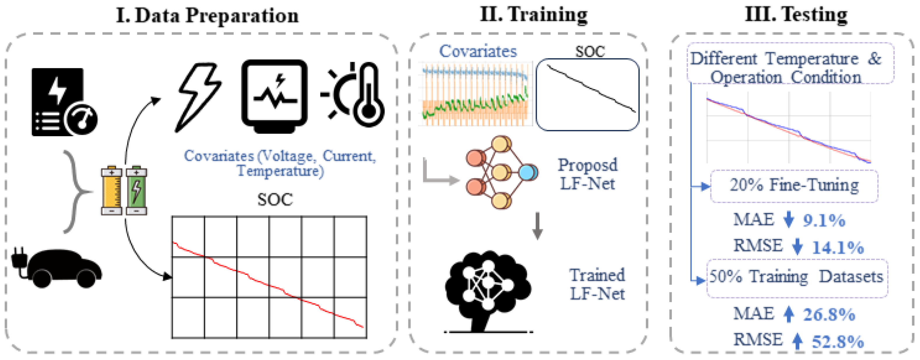
To clarify the end-to-end pipeline from data acquisition to evaluation and deployment, Figure 2 summarizes the workflow used in this study without depicting the internal network structure.

The LF-Net framework systematically integrates global trend information (Linear Module), multi-scale fluctuation characteristics (Fluctuation Module), rate-of-change features (Differential Module), and localized recent patterns (Local Enhancer Module). By explicitly modeling both the quasi-linear evolution and the superimposed fluctuation components through specialized modules, the model achieves high accuracy. The complementary nature of the information extracted by each module, combined through an adaptive fusion mechanism (Equation (16)) and weighted summation with local features (Equation (3)), enhances robustness and generalization capabilities for SOC estimation across diverse operating conditions.

3. Experimental Approval

3.1. Datasets

The data utilized for the experiments originates from a publicly accessible repository curated by the University of Maryland [33]. This repository encompasses battery operational data collected under three distinct standardized driving cycles: the Full Urban Driving Schedule (FUDS), the Dynamic Stress Test (DST), and the Supplemental Federal Test Procedure (US06). For each time step, the dataset provides measurements of voltage, current, and temperature, which function as input covariates for the model, alongside the corresponding SOC value, serving as the ground truth target.

To evaluate the model’s generalization performance, a specific data-partitioning strategy based on driving cycles and temperature conditions was implemented. The model training process exclusively employed data segments corresponding to the DST and US06 cycles. Model testing and performance assessment were conducted solely using data segments from the FUDS cycle. Furthermore, distinct thermal conditions were assigned to the training and testing sets to assess temperature robustness. The training dataset included measurements obtained at nominal ambient temperatures of 0 °C, 25 °C, 30 °C, and 50 °C. The testing dataset comprised measurements obtained at nominal ambient temperatures of 10 °C and 40 °C.

3.2. Experimental Approval Settings

The Experiments were operated on the NVIDIA (Santa Clara, CA, USA) 4070Ti Super hardware platform. Two metrics are used to evaluate the performance of models in the field of SOC estimation, as shown in Equations (17) and (18):

$$\mathrm{MAE}={\displaystyle \frac{1}{\tau }}\sum _{t=1}^{\tau }|{\mathrm{SOC}}_t-{\mathrm{SOC}}_t^{\ast }|$$

(17)

$$\mathrm{RMSE}=\sqrt{{\displaystyle \frac{1}{\tau }}\sum _{t=1}^{\tau }{({\mathrm{SOC}}_t-{\mathrm{SOC}}_t^{\ast })}^2}$$

(18)

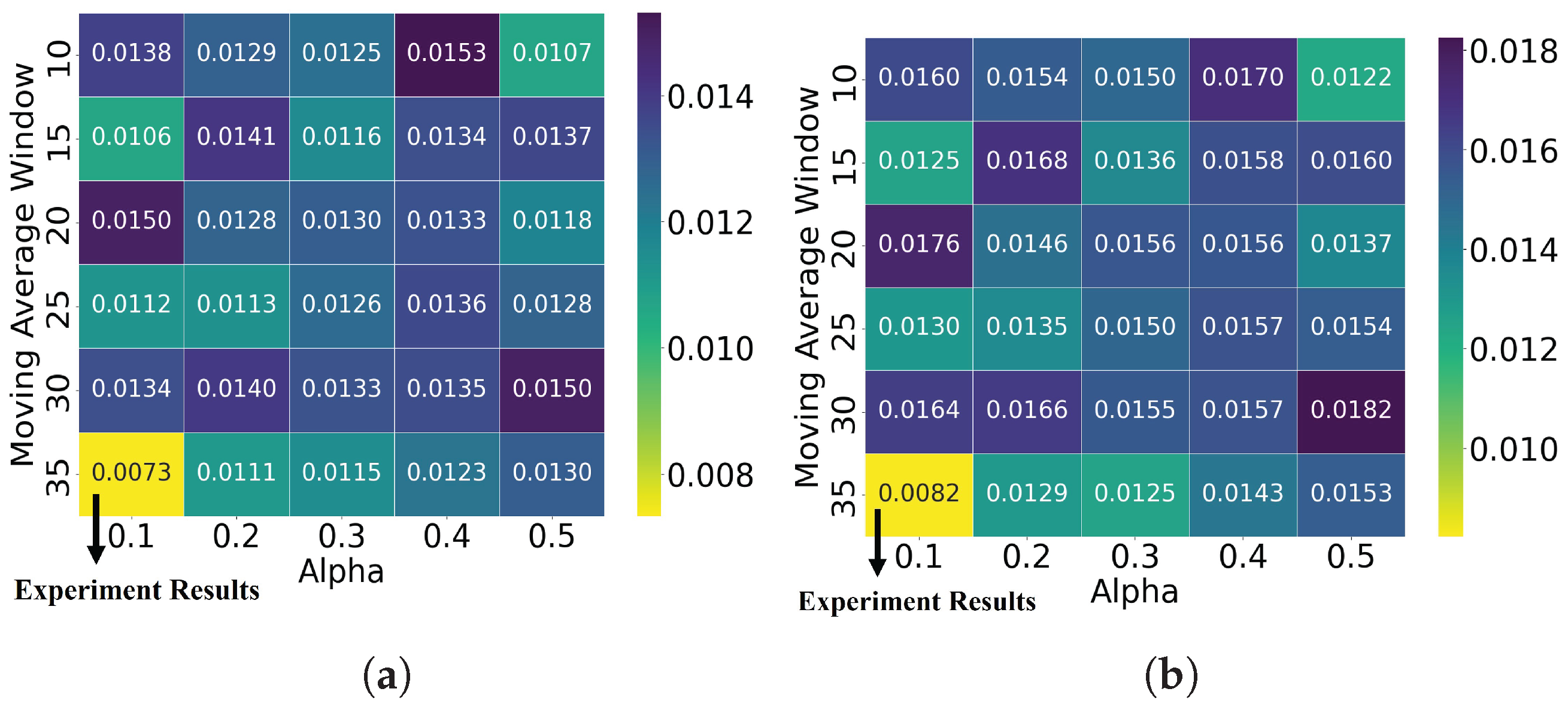
To optimize the hyperparameters of the proposed LF-Net, the moving-average window size and the local fluctuation enhancement weight (alpha) were selected for performance analysis. As shown in the hyperparameter optimization results (Figure 3), the moving average was sampled at six values ranging from 10 to 35 ([10, 15, 20, 25, 30, 35]), and alpha was sampled at five values ranging from 0.1 to 0.5 ([0.1, 0.2, 0.3, 0.4, 0.5]), resulting in 30 distinct configurations. The training data consisted of datasets from eight different operating conditions. The performance of each configuration was evaluated based on the MAE and RMSE achieved on the test dataset (40 °C on FUDS operating condition dataset was chosen here). From the experimental results, the configuration with a moving-average window size of 35 and an alpha value of 0.1 yielded the best performance, achieving the lowest RMSE (approximately 0.0082) and a corresponding MAE (approximately 0.0073).

3.3. Experimental Approval Results

3.3.1. Ablation Experiments

The performance of the LF-Net model and LF-Net without module 1–module 4 (module 1: Differential Feature Extraction Module; module 2: Local Enhancer Module; module 3: Fluctuation Module; module 4: Fusion Module) was compared. The training datasets and test datasets were the same as those in the hyperparameter experiment. The ablation experiment aimed to verify the contribution of each module to the model. The results are summarized in Figure 4:

3.3.2. Verification Experiments

The performance verification of LF-Net is demonstrated through the comparison plots shown in Figure 5. These visualizations present the alignment between actual SOC values and LF-Net predictions under different temperature conditions.

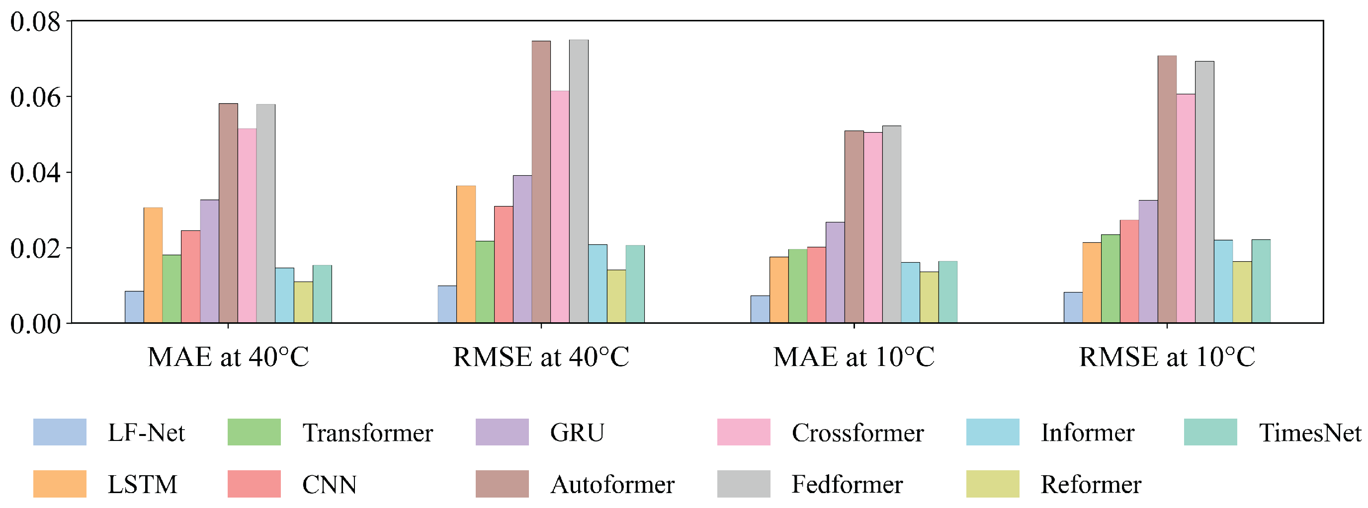
The experimental results, with the detailed metrics presented in

Table 1. Comparison of LF-Net and Baseline models on MAE and RMSE at 40 °C and 10 °C.

Type	LF-Net	LSTM [18]	Trans-Former [23]	CNN [17]	GRU [19]	Auto-Former [27]	Cross-Former [28]	Fed-Former [29]	Ham-Informer [26]	Re-Former [30]	TimesNet [25]
MAE at 40 °C	0.0085	0.0306	0.0181	0.0246	0.0327	0.0582	0.0515	0.0580	0.0147	0.0110	0.0154
RMSE at 40 °C	0.0099	0.0364	0.0218	0.0310	0.0391	0.0747	0.0615	0.0751	0.0208	0.0141	0.0206
MAE at 10 °C	0.0073	0.0176	0.0196	0.0202	0.0268	0.0510	0.0505	0.0523	0.0162	0.0136	0.0164
RMSE at 10 °C	0.0082	0.0214	0.0234	0.0274	0.0326	0.0709	0.0607	0.0694	0.0220	0.0163	0.0221

and a comparative visualization in Figure 6, confirm the effectiveness of the proposed LF-Net for SOC estimation. Under the 40 °C test condition, LF-Net achieves an MAE of 0.0085 and an RMSE of 0.0099. These figures represent a performance improvement over the best-performing baseline, Reformer, with a relative reduction of 22.7% in MAE and 29.8% in RMSE.

The model’s performance advantage is further extended under the 10 °C test condition, where it records an MAE of 0.0073 and an RMSE of 0.0082. This corresponds to a 46.3% reduction in MAE and a 49.7% reduction in RMSE when compared to the strongest baseline, Reformer. This data indicates that LF-Net maintains high accuracy and robustness across different operating temperatures, consistently outperforming a wide array of baseline models, from established architectures like LSTM and GRU to advanced Transformer variants.

As detailed in

Table 2. Comparison of LF-Net and Baseline models on parameters.

Type	LF-Net	LSTM [18]	Trans-Former [23]	CNN [17]	GRU [19]	Auto-Former [27]	Cross-Former [28]	Fed-Former [29]	Ham-Informer [26]	Re-Former [30]	TimesNet [25]
Parameters	15,925	5,263,873	152,385	1,621,441	3,948,033	1,259,009	945,584	494,337	1,657,345	663,553	4,689,474

, this level of predictive accuracy is achieved with high parameter efficiency. The LF-Net architecture consists of only 15,925 parameters, which is 89.5% lower than that of the most parameter-efficient baseline, Transformer (152,385 parameters). The combination of high precision and a lightweight structure makes LF-Net a suitable candidate for deployment on resource-constrained hardware typical in battery management systems. This efficiency can be attributed to the architecture’s strong inductive bias; the trend-fluctuation decomposition aligns with the inherent physical properties of the battery signal, facilitating more effective learning and reducing the risk of overfitting that can be present in larger, more generic models.

The finding that LF-Net achieves higher accuracy with fewer parameters can be attributed to the strong inductive bias of its architecture. The trend-fluctuation decomposition aligns with the signal’s physical properties, promoting efficient learning and mitigating overfitting. In contrast, larger generic models possess a higher risk of learning spurious correlations from the training data, which can impair generalization performance.

In the limited-data experiments, the exact training configurations are summarized in

Table 3. Training configurations under limited-data conditions.

Setting	Data Proportion	Selection Method	Epochs	Fine-Tuning
50% continuous subsets	50% per dataset	Continuous 25% datasets: front 50% 25% datasets: back 50% 50% datasets: random contiguous 50%	150	No
Light fine-tuning (20% datasets)	20% per dataset (additional datasets)	Continuous Random contiguous 20%	150	Yes

. Specifically, for the 50% dataset, training was performed on contiguous half-cycle segments per dataset (front/back/random contiguous per dataset), whereas for the 20% setting, training was performed using light fine-tuning with contiguous segments from DST/US06 at 10 °C and 40 °C. The corresponding performance results under these settings are reported in

Table 4. Robustness under limited data and effectiveness of light fine-tuning on FUDS test sets.

(a) Training on 50% Continuous Subsets			(b) Light Fine-Tuning
(Single-Cell)			(20% Continuous Segments from DST/US06 at 10 °C and 40 °C)
Metric	Full-Data Training	Continuous Subset (50%)	Metric	No Fine-Tuning	Light Fine-Tuning (20%)
MAE at 40 °C	0.0085	0.0105	MAE at 40 °C	0.0085	0.0080
RMSE at 40 °C	0.0099	0.0125	RMSE at 40 °C	0.0099	0.0088
MAE at 10 °C	0.0073	0.0095	MAE at 10 °C	0.0073	0.0064
RMSE at 10 °C	0.0082	0.0147	RMSE at 10 °C	0.0082	0.0068

.

Compared with full-data training, using a single cell and only a 50% continuous segment per condition yields a modestly higher MAE/RMSE at both temperatures. This indicates that reduced coverage increases difficulty while providing a meaningful stress test of rapid adaptation under limited data.

A short fine-tuning stage using only 20% continuous segments from DST/US06 at 10 °C and 40 °C improves generalization on FUDS without full retraining, suggesting that lightweight adaptation effectively mitigates cross-cycle/temperature mismatch and is practical for deployment.

4. Discussion

4.1. Results of This Study

LF-Net delivers strong accuracy at both 40 °C and 10 °C with a low MAE/RMSE while remaining lightweight (15,925 parameters) and suitable for embedded BMS. Ablation indicates that fluctuation and differential modules contribute most to performance. Under limited data, errors increase moderately; light fine-tuning reduces them. Errors concentrate near abrupt transitions; simple strategies improve responsiveness while preserving stability.

4.2. Practical and General Deployment Across Chemistries and Physical Implications

LF-Net modules have interpretations from battery physics that support generalization beyond LiFePO₄. The Linear Module aligns with coulomb counting and the average OCV-SOC slope; the multi-scale and differential pathways represent polarization, diffusion, and load transients; and the Local Enhancer uses the last segment. While these interpretations are intended as design rationales, generalization to other chemistries requires per-chemistry calibration of the OCV-SOC relationship and hysteresis/kinetics; nickel-rich cathodes may exhibit phase-change-associated voltage profiles that necessitate tailored preprocessing and fusion weighting.

For deployment, the following process should be carried out: use sliding-window inputs over voltage, current, temperature, and time, and set the window L according to the sampling rate and drive-cycle statistics. Standardize the inputs and, when needed, use a calibration layer with a monotonicity constraint or an OCV map defined on segments to align the predicted SOC to the rest-period OCV. Include temperature so that fusion or gating adapts across thermal regimes. When data exists, fuse the coulomb-counting residuals to correct long-horizon drift.

Set $\alpha$ as a function of context to increase sensitivity to fluctuations during segments with increased variance, and maintain stability otherwise. For BMS hardware, apply integer quantization to the FC and convolution layers and use streaming inference; the parameter count is 15,925. This deployment keeps the parameter count and supports operation across operating contexts [34,35].

4.3. Structural Disbalancing in Parallel-Connected Cells

In packs with parallel-connected cells, non-uniform aging and thermal gradients produce current splitting that differs across cells. The pack-level SOC can be expressed as a capacity-weighted combination of cell SOCs, where the weights change with internal resistance and temperature. Under such structural disbalancing, pack-level measurements reflect a time-varying mixture of cell dynamics. A model trained on balanced or single-cell data may exhibit bias when the mixture shifts.

Two practical mitigation paths are compatible with the present architecture: (i) Add imbalance proxies as auxiliary inputs, such as temperature spread ($\Delta T$ across cells or modules if available), short-horizon voltage/current variance, or impedance-related indicators estimated from routine diagnostics. These proxies can be concatenated to the combined feature vector before FusionNet so that the fusion adapts its weighting under imbalance. (ii) Condition the fusion weights on operating context by parameterizing $\alpha$ in Equation (3) as a function of the imbalance proxy and temperature, or by introducing a lightweight gating that prioritizes fluctuation-sensitive pathways when imbalance indicators are high.

If per-cell sensing is unavailable, pack-level proxies (e.g., variance in temperature sensors placed near parallel strings, or residuals between coulomb counting and model estimates) can serve as indirect indicators. When a new temperature or cycle is encountered, a short adaptation using a small continuous segment is expected to reduce bias without full retraining [36].

4.4. Local Fluctuation Capture

Figure 5 shows that while the global trend is accurately tracked, some high-frequency local fluctuations in the ground truth appear sharper than the model estimates. This attenuation is expected based on (i) the optimization objective (pointwise error), which favors stability; (ii) the moving-average decomposition and fusion, which are biased towards the linear trend; (iii) the LiFePO₄ OCV plateau, which reduces the sensitivity of voltage-to-SOC mapping within certain ranges; and (iv) pack-level measurement mixing and sensor noise.

To mitigate underfitting of local dynamics within the current architecture, three practical strategies are compatible with LF-Net:

(i)

Derivative-aware auxiliary loss, which encourages matching the rate of change shown in Equation (19):

$$\mathcal{L}={\mathcal{L}}_{\mathrm{SOC}}+{\lambda }_{\Delta }·{\displaystyle \frac{1}{\tau }}\sum _{t=2}^{\tau }|({\mathrm{S}\widehat{\mathrm{O}}\mathrm{C}}_t-{\mathrm{S}\widehat{\mathrm{O}}\mathrm{C}}_{t-1})-\left({\mathrm{SOC}}_t-{\mathrm{SOC}}_{t-1}\right)|.$$

(19)

(ii)

Context-conditioned fusion weighting $\alpha$ (Equation (3)), which increases the contribution of fluctuation-sensitive pathways under rapid dynamics, e.g., $\alpha =\sigma \left(W\left[z\right]+b\right)$ with $z=[\mathrm{Var}\left(X_{L-l+1:L}\right),T]$.

(iii)

Increasing the local window l and reinforcing a small-kernel convolutional branch to focus on short-horizon patterns.

These adjustments improve responsiveness to abrupt changes while preserving global stability; the choice of ${\lambda }_{\Delta }$, l, and the gating function balance noise amplification and fidelity to local transients.

5. Conclusions

A lightweight architecture for SOC estimation was presented that decomposes battery signals into a global trend and local fluctuations and fuses multi-branch representations. On FUDS test sets at 40 °C and 10 °C, the model yields MAEs/RMSEs of 0.0085/0.0099 and 0.0073/0.0082, respectively, with 15,925 parameters. The ablation indicates that fluctuation- and difference-based features materially affect accuracy.

The observed errors are concentrated near abrupt SOC changes. Within the present structure, short adaptation on a small continuous segment under the target condition can be applied to reduce bias without full retraining. For embedded deployment, the parameter size and branch-wise computation fit streaming inference on constrained platforms.

Future work will focus on two directions motivated by practical packs: (i) integrating imbalance proxies and state-of-health conditioning into the fusion to address structural disbalancing in parallel-connected cells, and (ii) enhancing the handling of short transients via adaptive fusion weights or context-conditioned gating while maintaining model compactness.

References

1. Saw, L.H.; Ye, Y.; Tay, A.A. Integration issues of lithium-ion battery into electric vehicles battery pack. J. Clean. Prod. 2016, 113, 1032–1045. [Google Scholar] [CrossRef]
2. Yang, X.G.; Liu, T.; Wang, C.Y. Thermally modulated lithium iron phosphate batteries for mass-market electric vehicles. Nat. Energy 2021, 6, 176–185. [Google Scholar] [CrossRef]
3. Kumar, J.; Neiber, R.R.; Park, J.; Ali Soomro, R.; Greene, G.W.; Ali Mazari, S.; Young Seo, H.; Hong Lee, J.; Shon, M.; Wook Chang, D.; et al. Recent progress in sustainable recycling of LiFePO4-type lithium-ion batteries: Strategies for highly selective lithium recovery. Chem. Eng. J. 2022, 431, 133993. [Google Scholar] [CrossRef]
4. Hannan, M.; Lipu, M.; Hussain, A.; Mohamed, A. A review of lithium-ion battery state of charge estimation and management system in electric vehicle applications: Challenges and recommendations. Renew. Sustain. Energy Rev. 2017, 78, 834–854. [Google Scholar] [CrossRef]
5. Manas, M.; Yadav, R.; Dubey, R.K. Designing a battery Management system for electric vehicles: A congregated approach. J. Energy Storage 2023, 74, 109439. [Google Scholar] [CrossRef]
6. Rao, Z.; Wang, S.; Zhang, G. Simulation and experiment of thermal energy management with phase change material for ageing LiFePO4 power battery. Energy Convers. Manag. 2011, 52, 3408–3414. [Google Scholar] [CrossRef]
7. Lu, P.; Li, C.; Schneider, E.W.; Harris, S.J. Chemistry, Impedance, and Morphology Evolution in Solid Electrolyte Interphase Films during Formation in Lithium Ion Batteries. J. Phys. Chem. C 2014, 118, 896–903. [Google Scholar] [CrossRef]
8. Fang, C.; Tran, T.N.; Zhao, Y.; Liu, G. Electrolyte decomposition and solid electrolyte interphase revealed by mass spectrometry. Electrochim. Acta 2021, 399, 139362. [Google Scholar] [CrossRef]
9. Tian, J.; Chen, C.; Shen, W.; Sun, F.; Xiong, R. Deep Learning Framework for Lithium-ion Battery State of Charge Estimation: Recent Advances and Future Perspectives. Energy Storage Mater. 2023, 61, 102883. [Google Scholar] [CrossRef]
10. Sun, S.; Guan, T.; Cheng, X.; Zuo, P.; Gao, Y.; Du, C.; Yin, G. Accelerated aging and degradation mechanism of LiFePO4/graphite batteries cycled at high discharge rates. RSC Adv. 2018, 8, 25695–25703. [Google Scholar] [CrossRef]
11. Snihir, I.; Rey, W.; Verbitskiy, E.; Belfadhel-Ayeb, A.; Notten, P.H. Battery open-circuit voltage estimation by a method of statistical analysis. J. Power Sources 2006, 159, 1484–1487. [Google Scholar] [CrossRef]
12. Zhou, Z.; Zhang, C. An extended Kalman filter design for state-of-charge estimation based on variational approach. Batteries 2023, 9, 583. [Google Scholar] [CrossRef]
13. Zheng, J.; Lu, J.; Amine, K.; Pan, F. Depolarization effect to enhance the performance of lithium ions batteries. Nano Energy 2017, 33, 497–507. [Google Scholar] [CrossRef]
14. Lu, Y.; Zhao, C.Z.; Huang, J.Q.; Zhang, Q. The timescale identification decoupling complicated kinetic processes in lithium batteries. Joule 2022, 6, 1172–1198. [Google Scholar] [CrossRef]
15. Issa, R.; Badr, M.M.; Shalash, O.; Othman, A.A.; Hamdan, E.; Hamad, M.S.; Abdel-Khalik, A.S.; Ahmed, S.; Imam, S.M. A data-driven digital twin of electric vehicle li-ion battery state-of-charge estimation enabled by driving behavior application programming interfaces. Batteries 2023, 9, 521. [Google Scholar] [CrossRef]
16. El Ancary, M.; Lassioui, A.; El Fadil, H.; El Asri, Y.; Hasni, A.; Yahya, A.; Chiheb, M. Hybrid Efficient Fast Charging Strategy for WPT Systems: Memetic-Optimized Control with Pulsed/Multi-Stage Current Modes and Neural Network SOC Estimation. World Electr. Veh. J. 2025, 16, 379. [Google Scholar] [CrossRef]
17. Lecun, Y.; Bottou, L.; Bengio, Y.; Haffner, P. Gradient-based learning applied to document recognition. Proc. IEEE 1998, 86, 2278–2324. [Google Scholar] [CrossRef]
18. Hochreiter, S.; Schmidhuber, J. Long Short-Term Memory. Neural Comput. 1997, 9, 1735–1780. [Google Scholar] [CrossRef]
19. Jiao, M.; Wang, D.; Qiu, J. A GRU-RNN based momentum optimized algorithm for SOC estimation. J. Power Sources 2020, 459, 228051. [Google Scholar] [CrossRef]
20. Hu, P.; Tang, W.; Li, C.; Mak, S.L.; Li, C.; Lee, C. Joint state of charge (SOC) and state of health (SOH) estimation for lithium-ion batteries packs of electric vehicles based on NSSR-LSTM neural network. Energies 2023, 16, 5313. [Google Scholar] [CrossRef]
21. El Fallah, S.; Kharbach, J.; Vanagas, J.; Vilkelytė, Ž.; Tolvaišienė, S.; Gudžius, S.; Kalvaitis, A.; Lehmam, O.; Masrour, R.; Hammouch, Z.; et al. Advanced state of charge estimation using deep neural network, gated recurrent unit, and long short-term memory models for lithium-Ion batteries under aging and temperature conditions. Appl. Sci. 2024, 14, 6648. [Google Scholar]
22. Sutanto, E.; Astawa, P.E.; Fahmi, F.; Hamid, M.I.; Yazid, M.; Shalannanda, W.; Aziz, M. Lithium-ion battery state-of-charge estimation from the voltage discharge profile using gradient vector and support vector machine. Energies 2023, 16, 1083. [Google Scholar] [CrossRef]
23. Vaswani, A.; Shazeer, N.; Parmar, N.; Uszkoreit, J.; Jones, L.; Gomez, A.N.; Kaiser, L.u.; Polosukhin, I. Attention is All you Need. In Proceedings of the Advances in Neural Information Processing Systems, Long Beach, CA, USA, 4–9 December 2017; Guyon, I., Luxburg, U.V., Bengio, S., Wallach, H., Fergus, R., Vishwanathan, S., Garnett, R., Eds.; Curran Associates, Inc.: Red Hook, NY, USA, 2017; Volume 30. [Google Scholar]
24. Zhou, H.; Zhang, S.; Peng, J.; Zhang, S.; Li, J.; Xiong, H.; Zhang, W. Informer: Beyond Efficient Transformer for Long Sequence Time-Series Forecasting. arXiv 2020, arXiv:2012.07436. [Google Scholar] [CrossRef]
25. Wu, H.; Hu, T.; Liu, Y.; Zhou, H.; Wang, J.; Long, M. TimesNet: Temporal 2D-Variation Modeling for General Time Series Analysis. arXiv 2023, arXiv:2210.02186. [Google Scholar]
26. Ren, W.; Xie, X.; Yi, Y.; Qi, C.; Huang, Y.; Feng, M.; Zheng, T. The LiFePO4 battery lifespan SoC estimation using Ham-Informer and internal pressure. J. Energy Storage 2024, 88, 111474. [Google Scholar] [CrossRef]
27. Wu, H.; Xu, J.; Wang, J.; Long, M. Autoformer: Decomposition Transformers with Auto-Correlation for Long-Term Series Forecasting. arXiv 2021, arXiv:2106.13008. [Google Scholar]
28. Wang, W.; Yao, L.; Chen, L.; Cai, D.; He, X.; Liu, W. CrossFormer: A Versatile Vision Transformer Based on Cross-scale Attention. arXiv 2021, arXiv:2108.00154. [Google Scholar]
29. Zhou, T.; Ma, Z.; Wen, Q.; Wang, X.; Sun, L.; Jin, R. FEDformer: Frequency Enhanced Decomposed Transformer for Long-term Series Forecasting. arXiv 2022, arXiv:2201.12740. [Google Scholar] [CrossRef]
30. Kitaev, N.; Kaiser, L.; Levskaya, A. Reformer: The Efficient Transformer. arXiv 2020, arXiv:2001.04451. [Google Scholar] [CrossRef]
31. Lim, B.; Ark, S.O.; Loeff, N.; Pfister, T. Temporal Fusion Transformers for interpretable multi-horizon time series forecasting. Int. J. Forecast. 2021, 37, 1748–1764. [Google Scholar] [CrossRef]
32. Zeng, A.; Chen, M.; Zhang, L.; Xu, Q. Are Transformers effective for time series forecasting? Proc. AAAI Conf. Artif. Intell. 2023, 37, 11121–11128. [Google Scholar] [CrossRef]
33. Battery Data|Center for Advanced Life Cycle Engineering. 2025. Available online: https://calce.umd.edu/ (accessed on 30 April 2025).
34. How, D.N.T.; Hannan, M.A.; Lipu, M.S.H.; Sahari, K.S.M.; Ker, P.J.; Muttaqi, K.M. State-of-Charge Estimation of Li-Ion Battery in Electric Vehicles: A Deep Neural Network Approach. IEEE Trans. Ind. Appl. 2020, 56, 5565–5574. [Google Scholar] [CrossRef]
35. Zheng, M.; Zhu, X.; Zheng, H.; Bo, Z.; Lu, J. Deployment strategies for Li-rich cathode materials in batteries. Nat. Energy 2025, 10, 789–792. [Google Scholar] [CrossRef]
36. Diao, W.; Pecht, M.; Liu, T. Management of imbalances in parallel-connected lithium-ion battery packs. J. Energy Storage 2019, 24, 100781. [Google Scholar] [CrossRef]
Figure 1. LF-Net architecture and data flow. Given an input sequence X R L × C (voltage, current, temperature, time), a moving-average decomposition (window w) is used to form a residual x short , while the original sequence feeds the linear branch. The Linear Module projects x long and x short with fully connected layers to capture the global evolution. The Fluctuation Module applies three parallel 1D convolutions with different kernel sizes to encode multi-scale local patterns. The Differential Feature Extraction Module operates on the first-order difference Δ X to highlight rapid transients. The Local Enhancer focuses on the last l steps via flatten-and-FC to emphasize the most recent dynamics. All features are concatenated and processed by FusionNet to obtain the main output; the final SOC estimate is a weighted sum of the main output and the local output with learnable weight α (Equation (3)). This design provides high accuracy with only 15,925 parameters, suitable for embedded BMS deployment.
Electronics 14 03643 g001
Figure 2. End-to-end workflow for SOC estimation, organized into three stages: (I) Data preparation: acquisition of voltage, current, temperature, and time; synchronization and cleaning; filtering and normalization; optional moving-average smoothing (window w); and sliding-window sample generation (length L, stride s). (II) Training: split by driving cycle and temperature into training and validation sets; optimize the SOC loss (optionally with a derivative-aware term); and apply early stopping and checkpointing. (III) Testing: apply the trained model on sliding windows in a streaming manner; perform optional light post-processing; and report MAE and RMSE, with an optional export path for quantized, embedded deployment in BMS.
Electronics 14 03643 g002
Figure 3. Hyperparameter tuning results for LF-Net: (a) MAE and (b) RMSE across moving-average window sizes and local enhancement weights (Alpha); both metrics are minimized at window size 35 and Alpha 0.1.
Electronics 14 03643 g003
Figure 4. MAE and RMSE results for the ablation study on the 40 °C FUDS test set. The ‘LF-Net (Full Model)’ serves as the performance baseline. Each subsequent bar illustrates the performance degradation (i.e., increase in MAE and RMSE) upon removing a specific module. The results demonstrate that all modules contribute positively to the model’s accuracy, with the removal of the Fluctuation and Differential modules causing the most significant performance drop.
Electronics 14 03643 g004
Figure 5. Comparison of actual SOC and LF-Net estimates on FUDS test sets: (a) 10 °C and (b) 40 °C. The predictions closely align with the ground truth across both temperatures, demonstrating accuracy under significant fluctuations and robustness at higher temperatures.
Electronics 14 03643 g005
Figure 6. Comparative performance analysis of LF-Net against ten baseline models on the FUDS test sets. The chart displays the MAE and RMSE at both 40 °C and 10 °C. LF-Net consistently achieves the lowest error across all four evaluation metrics, demonstrating LF-Net’s superior accuracy and robustness under different thermal conditions.
Electronics 14 03643 g006