An Automatic Brain Cortex Segmentation Technique Based on Dynamic Recalibration and Region Awareness

Abstract

To address the limitations in the accuracy of current cerebral cortex structure segmentation methods, this study proposes an automatic segmentation network based on dynamic recalibration and region awareness. The network is an improved version of the classic U-shaped architecture, incorporating a Dynamic Recalibration Block (DRB) and a Region-Aware Block (RAB). The DRB enhances important feature channels by extracting global feature information across channels, computing the significance weights via a two-layer fully connected network, and applying these weights to the original feature maps for dynamic feature reweighting. Meanwhile, the RAB integrates spatial positional information and captures both global and local context across multiple dimensions. It recalibrates features using dimension-specific weights, enabling region-aware feature association and complementing the DRB’s function. Together, these components enable efficient and accurate segmentation of brain structures. The proposed DRA-Net model effectively overcomes the accuracy–efficiency trade-off in cortical segmentation through multi-scale feature fusion, dual attention mechanisms, and deep feature extraction strategies. Experimental results demonstrate that DRA-Net achieves an average Dice score of 91.35% across multiple datasets, outperforming segmentation atlases based on methods such as U-Net, QuickNAT, and FastSurfer.

1. Introduction

As the most complex neural center of the human body, the brain serves as the material foundation for advanced human cognitive functions. A wealth of research in neuroscience has demonstrated that structural abnormalities in various cortical regions of the brain are closely linked to the onset and progression of neurological disorders such as Alzheimer’s disease and Parkinson’s disease [1,2,3,4,5,6]. The cerebral cortex functions similarly to an intricate neural map, enabling the precise localization of brain functional areas. This capability provides critical support for early diagnosis and dynamic monitoring of neurological conditions, while also offering a robust anatomical and functional basis for the development of personalized treatment strategies. Moreover, it opens new avenues for exploring brain function mechanisms and enhancing the diagnosis and treatment of neurological diseases [5,7,8,9]. Accurately identifying these structural abnormalities first requires precise segmentation of the cerebral cortex into distinct regions—much like accurately marking every street on a satellite map, where only sufficiently fine-grained delineation can reveal subtle changes. Therefore, the development of efficient and accurate cortical segmentation methods is essential not only for supporting clinical diagnosis and personalized therapy, but also for laying a solid foundation for advancing our understanding of brain function.

Manual segmentation has long been regarded as the “gold standard” in brain parcellation. In 1909, neuroanatomist Korbinian Brodmann employed cellular staining techniques to subdivide the cerebral cortex into 52 functional areas—now widely known as Brodmann areas—based on the morphology and arrangement of cortical neurons [10]. This pioneering work established the first systematic anatomical framework for cortical functional regions and laid the foundation for the development of neuroimaging and cognitive neuroscience. In 1988, Talairach and Tournoux expanded upon Brodmann’s framework by performing serial sectioning on the frozen brain of a 60-year-old European female cadaver [11]. Through precise manual segmentation and incorporation of Brodmann’s functional labels, they successfully mapped the anatomical–functional regions of subcortical nuclei and subsequently developed the first three-dimensional coordinate system—the Talairach coordinate system, also known as the Talairach–Tournoux standard space [12]. This system defines its origin at the intersection of the midsagittal plane and the anterior–posterior axis of the brain, using the line between the anterior and posterior commissures as its horizontal reference, thereby creating a standardized spatial framework. Today, this coordinate system continues to serve as the foundational spatial model for widely used neuroimaging analysis tools such as SPM [13] (Statistical Parametric Mapping), FSL [14] (FMRIB Software Library), and AFNI [15] (Analysis of Functional NeuroImages), and plays a crucial role in clinical surgical planning by supporting spatial normalization and cross-study comparison. Nevertheless, traditional manual segmentation methods are time-consuming, labor-intensive, and highly dependent on the operator’s expertise and subjective judgment, resulting in substantial inter-operator variability and limited reproducibility [16].

With the rapid advancement of non-invasive brain imaging technologies, semi-automated brain segmentation methods have gained significant momentum. In 2002, Tzourio-Mazoyer et al. developed a method based on the Colin27 brain atlas, employing anatomical labeling tools and image processing algorithms to manually delineate gyral and sulcal structures on axial slices [17]. This approach partitioned each hemisphere into 45 functional regions and provided critical reference support for widely used MRI analysis tools such as SPM and MRIcron [18]. In 2006, Desikan et al. proposed a hybrid method that combined automatic sulcal–gyral identification with manual correction by neuroanatomical experts, ultimately expanding cortical segmentation to 68 functional regions [19]. Due to its high anatomical accuracy, this method became the standard parcellation scheme for platforms such as FreeSurfer [20] and CAT [21]. In 2010, the Destrieux team further refined segmentation granularity by integrating multimodal data—including structural and functional MRI, EEG, and MEG—and applying iterative algorithmic optimization combined with expert annotations, resulting in a fine-grained parcellation of 74 functional regions per hemisphere [22]. Despite improvements over fully manual approaches, these semi-automated methods remain limited by high dependence on human intervention, low processing efficiency, and poor adaptability to inter-individual anatomical variability. These limitations highlight the urgent need for more intelligent and efficient fully automated brain segmentation techniques to achieve further breakthroughs.

With the growing demand for efficient and precise brain segmentation in neuroscience research, fully automated segmentation techniques have rapidly evolved. These methods require no human intervention and are capable of achieving individualized brain region delineation, significantly enhancing processing efficiency. In 2017, Raghav et al. pioneered the use of BrainSegNet [23], which leveraged the multi-dimensional feature extraction capabilities of convolutional neural networks to perform automatic cortical boundary segmentation based on deep learning for the first time. Building on this, a series of breakthroughs in deep learning-based brain region segmentation emerged. In 2018, Christian et al. developed DeepNAT [24], an end-to-end model that incorporated Laplace-Beltrami operator features to segment 25 brain structures. In 2019, Nassir et al. introduced QuickNAT [25], which employed three parallel 2D fully convolutional networks and improved segmentation accuracy across 27 brain regions. In 2020, Mansencal and colleagues proposed the AssemblyNet [26], which innovatively integrated prior knowledge from nonlinear registration and leveraged multi-scale feature propagation to achieve more accurate, individualized segmentation. Between 2020 and 2023, the Henschel team continued to enhance QuickNAT, releasing the FastSurfer series of models [27], which provided an efficient solution for large-scale automated processing of neuroimaging data. These models, driven by powerful feature learning capabilities and complex network architectures, enabled fine-grained and fully automated segmentation, marking a new phase of intelligent and automated development in the field. However, existing deep learning-based segmentation models still exhibit considerable variability in accuracy when processing medical image regions with complex structures or ambiguous boundaries [27], and some network designs are redundant, resulting in low inference efficiency that further limits their applicability in real-time clinical scenarios. For example, as a classic baseline, U-Net often demonstrates insufficient feature representation and blurred boundaries in low-contrast regions. While QuickNAT and FastSurfer show high efficiency in large-scale data processing, their reliance on local features neglects cross-channel global information interactions, leading to reduced spatial sensitivity in complex structural regions and insufficient capture of intricate cortical folds. These issues indicate that future research should focus on enhancing cross-channel feature modeling and spatial structure awareness while maintaining efficiency, to achieve more accurate and robust automated segmentation of the cerebral cortex.

To address the above challenges, this study proposes a high-precision automatic segmentation network that integrates dynamic recalibration and region-aware mechanisms. Based on the classical U-shaped architecture, the network introduces two key components: the Dynamic Recalibration Block (DRB) and the Region-Aware Block (RAB). The DRB module extracts local features while integrating global inter-channel information, enabling the network to adaptively learn semantic weight distributions across channels. This enhances the flow of relevant features and strengthens key information representations. The RAB module incorporates spatial position encoding and multi-scale contextual cues to recalibrate feature responses, allowing for joint modeling of local details and global structural dependencies. This significantly improves the network’s ability to delineate complex anatomical boundaries in the cerebral cortex. Architecturally, the model employs a collaborative multi-view 2D segmentation strategy across three orthogonal planes, preserving 3D structural integrity while maintaining computational efficiency. Furthermore, the network is trained via a fully end-to-end pipeline, significantly reducing reliance on manual annotations and improving generalization performance under limited training data. Contributions:

• A novel dual-module design (DRB + RAB) is proposed to enhance feature discrimination and structural awareness for accurate cortical segmentation.
• A lightweight, multi-plane segmentation strategy is employed to strike a balance between segmentation performance and computational efficiency.
• The training framework demonstrates strong generalization and robustness in small-sample scenarios.
• The proposed method offers a scalable and practical solution for clinical applications such as disease localization and neurosurgical navigation.

2. Materials and Methods

2.1. Datasets

This study utilizes the Mindboggle-101 dataset [28] (https://osf.io/nhtur/, accessed on 24 July 2024), which integrates multiple sub-datasets—including Colin27, HLN, MMRR, NKI-RS, NKI-TRT, Twins, and OASIS-TRT—and is currently the largest, most comprehensive, and freely accessible human brain anatomical imaging database. The dataset is annotated according to the Desikan–Killiany–Tourville (DKT) protocol, ensuring consistency and anatomical accuracy of the labels. A total of 98 T1-weighted MRI scans from healthy individuals were used for this study. To ensure the reliability of automated segmentation, 78 subjects from the Colin27, HLN, MMRR, NKI-RS, NKI-TRT and Twins datasets were selected, and all images were resampled to isotropic voxels of 1 mm³ using trilinear interpolation. These subjects were used for model training and validation through five-fold cross-validation, while the remaining 20 subjects from the OASIS-TRT subset served as an independent test set. There was no overlap between subsets, and the risk of potential data leakage was fully avoided. Further details of the dataset composition are provided in

Table 1. Participant information.

Experiment	Dataset Name	Sample Size	Age Range (Years)	Mean Age ± SD (Years)	Male/ Female	Left-/Right-Handed
Training and Validation	NKI-RS	22	20–40	26 ± 5.2	12/10	1/21
	NKI-TRT	20	19–60	31.4 ± 11.1	14/6	3/15
	MMRR	21	22–61	31.8 ± 9.2	11/10	3/18
	HLN	12	23–39	27.8 ± 4.6	6/6	0/12
	Colin27	1	33	33	1/0	0/1
	Twins	2	41	—	0/2	0/2
Independent Test	OASIS-TRT	20	19–34	23.4 ± 3.9	8/12	0/20

.

2.2. Data Preprocessing

To provide effective data labels for subsequent model training, all data underwent preprocessing. In this study, preprocessing was performed using FreeSurfer (https://surfer.nmr.mgh.harvard.edu/fswiki, accessed on 8 October 2023), following the steps illustrated in Figure 1:

(1)

Skull stripping: brain and non-brain tissues were separated using grayscale thresholding and edge detection techniques to remove the skull, resulting in clean images for further brain analysis.

(2)

Normalization: A non-rigid registration algorithm was employed to align all brain images to a common standard space. This step mitigates individual variability and enables cross-subject comparison of brain structures.

(3)

Tissue segmentation: brain tissues (gray matter, white matter, and cerebrospinal fluid) were labeled using a Bayesian classification approach based on the Expectation-Maximization (EM) algorithm, ensuring efficiency and accuracy in subsequent segmentation processes.

(4)

White matter segmentation: a gradient-based watershed algorithm combined with morphological operations was applied to precisely segment white matter, providing fine-grained structural information for brain parcellation.

(5)

Cortical extraction: the cerebral cortex was extracted using algorithms based on gradient and geometric morphology, allowing accurate differentiation between cortical and subcortical structures.

(6)

Spherical registration: a spherical registration algorithm was used to map the cortical surface onto a standard spherical template, thereby reducing morphological differences across individuals.

(7)

Label annotation: finally, automatic labeling was performed using the DKT (Desikan–Killiany–Tourville) atlas to generate the training labels required for the model.

2.3. Methods

2.3.1. Cortical Structural Network Architecture

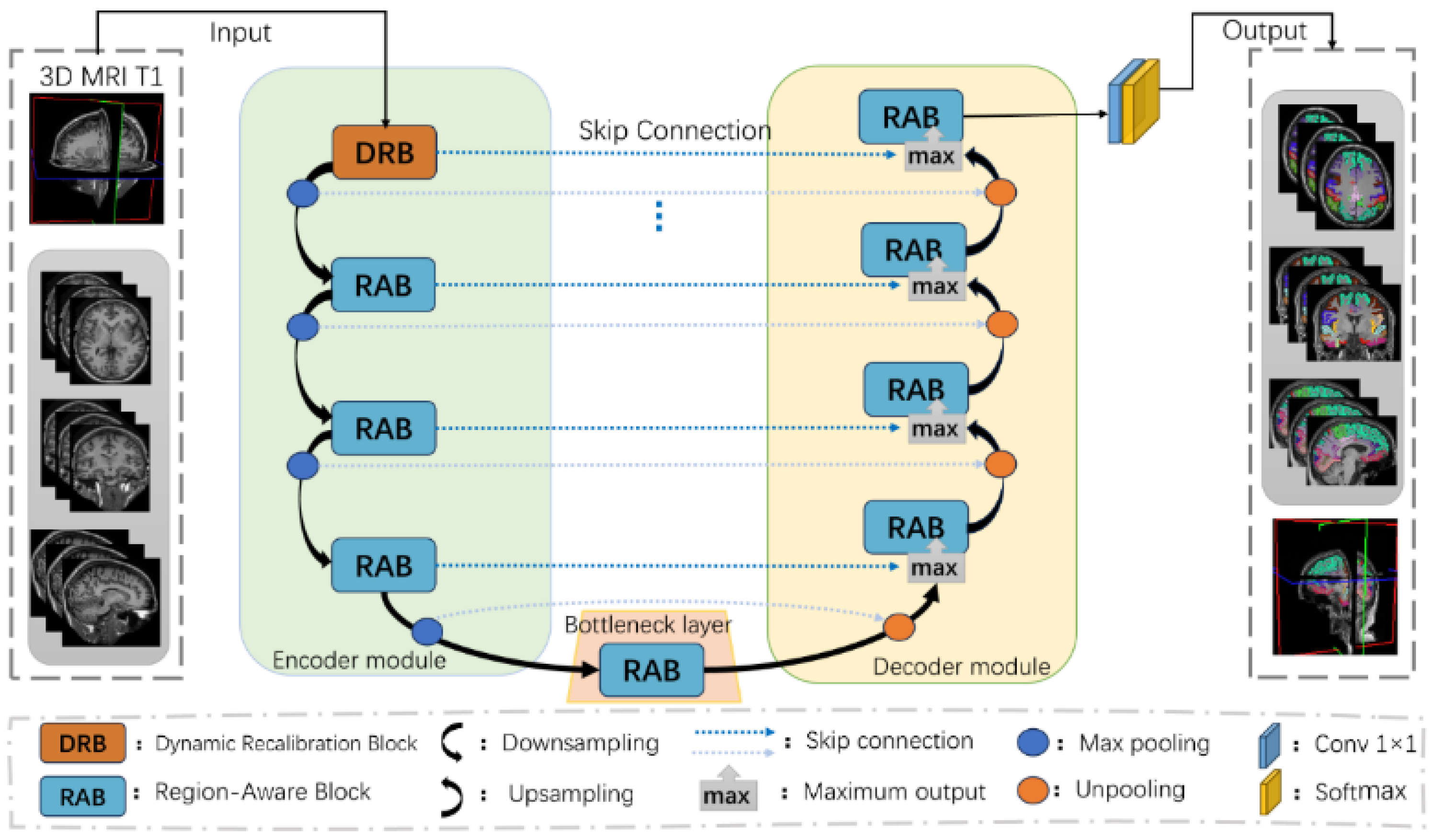
Figure 2 illustrates the proposed deep learning network for 3D medical image segmentation, named DRA-NET. Based on a U-shaped architecture, DRA-NET incorporates a Dynamic Recalibration Block (DRB) and multiple Region-Aware Blocks (RABs) to enhance segmentation performance (see Figure 3). To balance model accuracy and computational efficiency, the framework employs a unique 2D slice-based processing strategy: the preprocessed 3D data are decomposed into sequential 2D slices along the coronal, sagittal, and axial planes, which are then used as inputs to the encoder. This approach significantly reduces computational cost while preserving the spatial continuity of the 3D brain structure. The 2D slices are first processed by the encoder for feature extraction, followed by a bottleneck layer that captures long-range spatial dependencies. The decoder then progressively reconstructs the feature representations, and the final cortical structure segmentation is achieved through a convolutional layer and a softmax activation function, producing a detailed structural brain map.

Notably, each input to the model is not a single slice but a set of seven consecutive slices, including the target slice and its three adjacent slices above and below, thus partially preserving the cross-slice 3D context. Moreover, we train separate networks on the coronal, axial, and sagittal anatomical planes, and the final segmentation is obtained by averaging the probability maps from all three views to compensate for the limitations of single-view inputs. The following sections focus on the design principles and implementation details of the DRB and RAB modules.

2.3.2. Dynamic Recalibration Block (DRB)

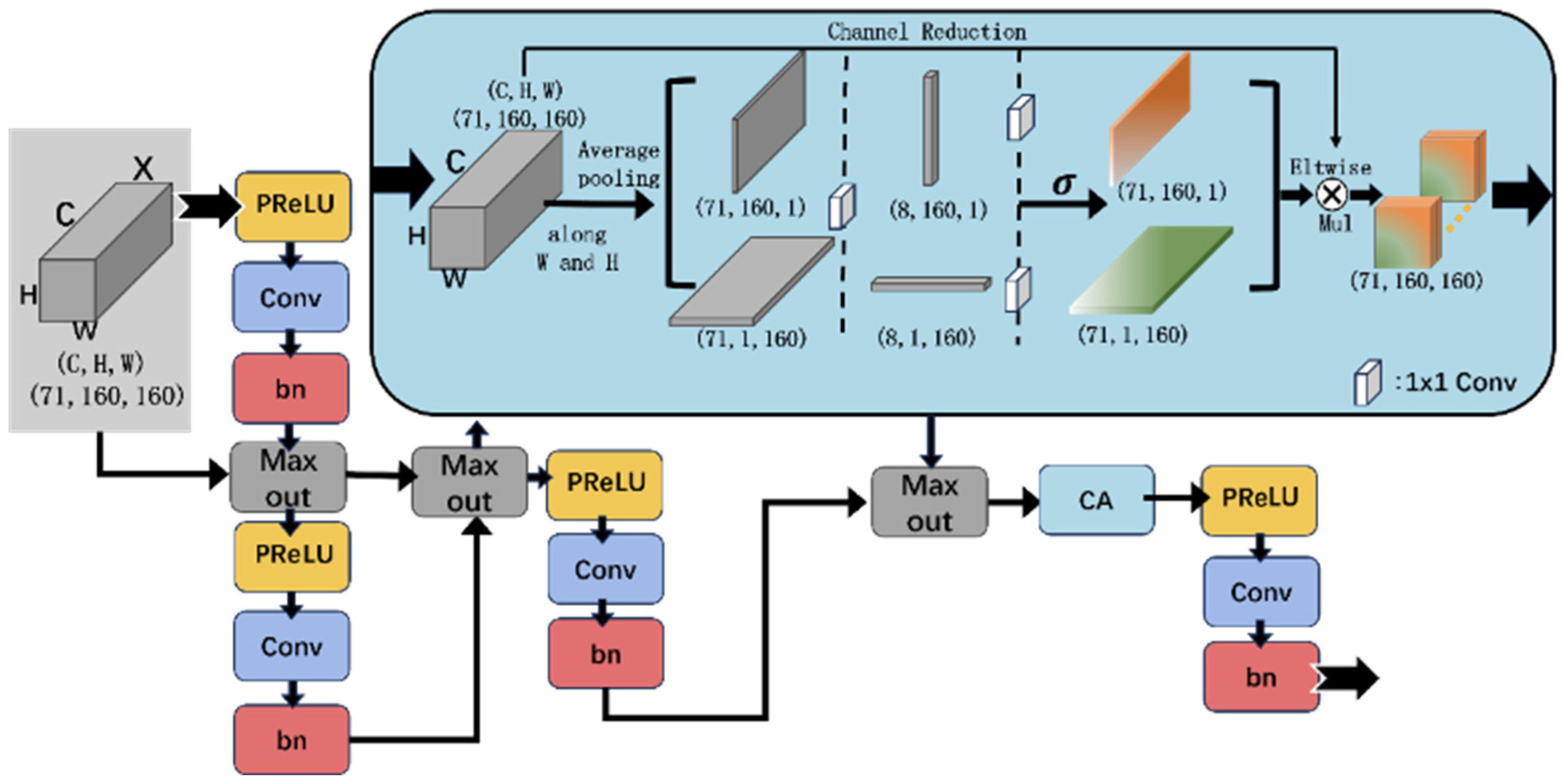
In the field of deep learning-driven medical image analysis, precise feature extraction and effective feature recalibration are crucial for improving diagnostic accuracy and reliability. This study proposes the Dynamic Recalibration Block (DRB), illustrated in Figure 3, to enhance the network’s ability to extract important feature information while suppressing irrelevant signals, thereby achieving more accurate and reliable segmentation of target regions in medical images.

The input to the DRB consists of sequential 2D slices from three orthogonal views: coronal, sagittal, and axial planes. These slices first pass through several normalization layers and convolutional layers to produce the initial feature map X. Subsequently, an efficient channel attention mechanism, namely the efficient channel attention (ECA) [29], is introduced to adaptively recalibrate the weights of different channel features. Key features are then further integrated using Maxout [30] and additional convolutional layers.

The efficient channel attention (ECA) mechanism is employed to dynamically recalibrate the importance of different channel features through local information interaction. Specifically, global average pooling (GAP) is first applied to extract global features summarizing the entire input, as detailed in Equation (1). The ECA does not perform dimensionality reduction or compression, thereby preserving the integrity of the features.

$$z_c={\displaystyle \frac{1}{H\times W}}\sum _{i=1}^H\sum _{j=1}^W{x}_{i,j}^c$$

(1)

Here, $x_{i,j}^c$ represents the value at position $(i,j)$ in the c-th channel of the input feature map. H and W denote the height and width of the feature map, respectively. $z_c$ is the global average value of the c-th channel. Unlike traditional channel attention mechanisms, ECA does not use fully connected layers or dimensionality reduction. Instead, it employs a 1D convolution with a kernel size of 3 for local cross-channel interaction. This approach effectively captures the dynamic dependencies between adjacent channels while maintaining computational efficiency and avoiding information loss caused by dimensionality reduction. Finally, channel weights are computed using a sigmoid activation function and applied to the original feature map via element-wise multiplication for dynamic recalibration. This adaptive optimization under varying input data is mathematically expressed in Equation (2).

$$x_c^{\prime }=x_c\cdot {\displaystyle \frac{1}{1+e^{-s_c}}}, \forall c\in \left\{\mathrm{1,2},\dots ,C\right\}$$

(2)

where $s_c$ denotes the output of the 1D convolution, $x_c$ represents the input feature map value in channel c, and $x_c^{\prime }$ is the recalibrated (weighted) feature map.

Finally, the output feature map of the DRB, denoted as $F_{out}$, is obtained through two convolutional layers, each followed by batch normalization and PReLU nonlinear activation, as well as two Maxout operations. This process is mathematically described in Equation (3).

$$F_{out}=Convs\left({\left[y_{ij}\right]}_{i,j=1}^{H,W,C}\right),y_{ij}=max s_{ij}^1,s_{ij}^2,\dots ,s_{ij}^C$$

(3)

2.3.3. Region-Aware Block (RAB)

The Dynamic Recalibration Block (DRB) achieves dynamic channel-wise attention by globally weighting each channel’s feature importance but does not consider spatial positional information. Therefore, we propose the Region-Aware Block (RAB), illustrated in Figure 4. The RAB applies pooling along two spatial dimensions of the features, enabling the network to capture both global context and local spatial continuity. Moreover, considering the high computational cost of high-resolution medical images, the RAB utilizes channel attention [31] (CA) to aggregate global information separately along the horizontal (width, W) and vertical (height, H) directions via one-dimensional operations, thereby avoiding the expensive computation of attention weights between all global pixels.

The RAB module is capable of capturing long-range dependencies in high-resolution medical images (such as MRI slices), thereby enhancing the overall anatomical consistency across brain regions. At the same time, it preserves spatial orientation information, enabling the network to better recognize variations in cortical structures. This leads to improved segmentation accuracy in low-contrast regions and reduces the likelihood of missegmentation. Moreover, the design avoids excessive computational overhead, keeping the model complexity relatively low.

Specifically, the feature map X is first processed by convolutional layers similar to those in Equation (3) to effectively extract meaningful features. A Maxout operation is then applied to select the most informative responses. Subsequently, average pooling is performed separately along the height (H) and width (W) dimensions, followed by weighted fusion to combine information from both directions and enhance the representational capacity of the features. Finally, the output feature representation is obtained using the operations described in Equation (3).

For the input feature map X with dimensions (71, 160, and 160), the spatial resolution remains unchanged after passing through the first two Maxout operations and convolutional layers. Global average pooling is then applied separately along the height (H) and width (W) dimensions, resulting in directional feature statistics of size (71, 160, and 1) and (71, 1, and 160), respectively. During the feature compression stage, both sets of features are passed through a shared 1 × 1 convolutional layer to perform channel-wise compression with a reduction ratio of $r=9$, producing the compressed representations $f_h$ and $f_w$. Sigmoid activation functions are subsequently used to generate the spatial attention weights ${\mathsf{\alpha }}_h$ and ${\mathsf{\alpha }}_w$, which are applied to the original feature map through channel-wise weighted multiplication for dynamic adjustment. The final output feature map of the RAB, $F_{out}$, is computed according to Equation (3).

It is also worth noting that the first layer of the network’s encoder accepts a 7-channel input and gives a 71-channel output, using the DRB module that acts directly on the original images. All subsequent encoder layers and all decoder layers have 71 input and output channels, enabled by the RAB module that acts on the feature maps. The encoder employs max-pooling for downsampling, while the decoder uses the corresponding maximum unpooling for upsampling. For more details, please refer to the source code (https://github.com/GaodengFan/Seg, accessed on 28 July 2025) and Supplementary Table S1.

2.4. Loss Function

This study employs Dice loss and cross-entropy loss to guide the training process.

${\mathcal{L}}_{dice}$: The Dice coefficient measures the overlap between the predicted region and the ground truth. A lower Dice loss value indicates better overlap and thus more accurate segmentation. The Dice loss is mathematically defined in Equation (4).

$${\mathcal{L}}_{dice}=1-{\displaystyle \frac{2\mid P\cap G \mid }{\mid P\mid +\mid G \mid }}$$

(4)

where $P$ denotes the predicted segmentation region by the model, and $G$ represents the ground truth region.

${\mathcal{L}}_{ce}$: Cross-entropy loss measures the difference between the predicted class distribution and the ground truth labels. A lower cross-entropy loss indicates a smaller discrepancy between the model’s predictions and the true labels, reflecting a better model fit. The cross-entropy loss is mathematically defined in Equation (5).

$${\mathcal{L}}_{ce}=-\sum _{c=1}^C{y}_i\mathit{log}\left({\widehat{y}}_c\right)$$

(5)

where $C$ represents the number of classes, ${\mathrm{y}}_c$ is the ground truth label for class $C$ (0 or 1), and ${\widehat{y}}_c$ denotes the predicted probability for class $C$.

Therefore, the total loss function is defined as $\mathcal{L}=\mathsf{\alpha }{\mathcal{L}}_{dice}+\beta {\mathcal{L}}_{ce}$, where the experimental settings use $\mathsf{\alpha }=1$ and $\beta =1$.

2.5. Evaluation Metrics

This study evaluates the effectiveness and performance of the prefrontal cortex structural maps constructed using DRA-NET by employing the following metrics: mean intersection over union (MIoU), mean recall, mean precision, and Dice coefficient.

MIoU: This metric represents the average intersection over union between the predicted segmentation region and the ground truth region. It is mathematically defined in Equation (6).

$$MIoU={\displaystyle \frac{1}{N}}\sum _{i=1}^{N}N{\displaystyle \frac{Intersection(P_i,G_i)}{Union(P_i,G_i)}}={\displaystyle \frac{\mid P_i\cup G_i \mid }{\mid P_i\cap G_i \mid }}$$

(6)

where $P_i$ denotes the predicted region for class $i$, $G_i$ represents the ground truth region for class $i$, $N$ is the total number of classes, and ${IoU}_i$ is the intersection over union for class $i$.

Mean recall: This metric evaluates the completeness of the model’s identification of true anatomical regions, measuring the proportion of correctly segmented pixels within each target structure. In this study, the original brain MRI images are divided into distinct anatomical regions, and the model is trained to accurately assign each voxel to its corresponding brain region label. The recall metric reflects the extent of under-segmentation (i.e., missed regions) when identifying anatomical structures. It is mathematically defined in Equation (7).

$$Mean Recall={\displaystyle \frac{1}{N}}\sum _{i=1}^N{\displaystyle \frac{{True Positives}_i}{{True Positives}_i+{False Negatives}_i}}$$

(7)

where ${True Positives}_i$ refers to the number of true positives for class $i$, ${False Negatives}_i$ refers to the number of false negatives for class $i$, and $N$ is the total number of classes.

Mean precision: This metric evaluates the accuracy of the model’s predictions for positive samples; that is, the proportion of correctly predicted regions that actually belong to a given anatomical structure. It is mathematically defined in Equation (8).

$$Mean Precision={\displaystyle \frac{1}{N}}\sum _{i=1}^N{\displaystyle \frac{{True Positives}_i}{{True Positives}_i+{False Positives}_i}}$$

(8)

where ${True Positives}_i$ denotes the number of true positives for class $i$, ${False Positives}_i$ denotes the number of false positives for class $i$, and $N$ is the total number of classes.

Hausdorff distance (HD): Hausdorff distance is a metric used to measure the maximum deviation between two point sets—such as the predicted segmentation and the ground truth. It quantifies the worst-case error by identifying the greatest distance from a point in one set to the closest point in the other set. The mathematical definition is given in Equation (9).

$$\begin{gathered} H\left(A,B\right)=max\left(h\left(A,B\right),h\left(B,A\right)\right), \\ where h(A,B)=\underset{a\in A}{max}\left(\underset{b\in B}{min}‖a-b‖\right) \end{gathered}$$

(9)

where $\mathrm{h}(\mathrm{A},\mathrm{B})$ represents the maximum of these minimum distances across all points in set A, indicating the point in A that is farthest from B. By repeating this process in the reverse direction—swapping A and B—and taking the maximum of the two values, we obtain the Hausdorff distance, which reflects the greatest discrepancy between the two sets.

Mean loss: The mean loss represents the average value of the loss function throughout the entire training process. It reflects the overall performance of the model in optimizing the objective function. A lower mean loss indicates a smaller overall prediction error and better global fitting capability of the model. The mathematical formulation is given by Equation (10).

$$\mu L={\displaystyle \frac{1}{N}}\sum _{i=1}^N{L}_i$$

(10)

where ${\mathrm{L}}_i$ denotes the loss value at the $i$-th iteration, and $N$ is the total number of iterations.

Loss volatility quantifies the degree of fluctuation in the loss curve. Lower volatility indicates smoother changes in the loss function, reflecting higher training stability. The mathematical definition is given by Equation (11).

$$\sigma L=\sqrt{{\displaystyle \frac{1}{N}}\sum _{i=1}^N{(L_i-\mu L)}^2}$$

(11)

where $\sigma L$ represents the standard deviation of the loss values, indicating the degree of dispersion of the losses relative to the mean. A smaller $\sigma L$ suggests that the loss values are more consistently distributed around the average, implying greater training stability.

2.6. Experimental Setup

The proposed method was implemented in PyTorch(version 1.12.1) and trained on a workstation equipped with an NVIDIA RTX 4090 GPU (24 GB memory; ASUS, Taipei, China). The network was trained for 100 epochs with a batch size of 8. The initial learning rate was set to 0.01, with a weight decay of 1 × 10⁻⁴, and it was decayed by 95% every five epochs. The Adam optimizer was employed to update and fine-tune the model parameters.

3. Experimental Results

3.1. Determination of the Number of RAB Modules

The number of network layers serves as a key parameter that directly affects both model performance and computational overhead. To identify the optimal network depth for DRA-Net, we conducted a systematic evaluation of architectures ranging from 1 to 6 layers. Due to the computational cost of deeper networks exceeding our available resources, configurations with more than six layers were not explored. As shown in

Table 2. Quantitative performance analysis of different RAB module depths.

Number of Layers	MIoU	Recall	Precision	Loss Total	Time (h)
1	0.66 ± 0.07	0.79 ± 0.06	0.79 ± 0.04	0.90 ± 0.07	38.14
2	0.73 ± 0.03	0.85 ± 0.02	0.83 ± 0.03	0.85 ± 0.03	41.02
3	0.72 ± 0.05	0.84 ± 0.05	0.83 ± 0.03	0.84 ± 0.06	41.55
4	0.73 ± 0.03	0.85 ± 0.02	0.83 ± 0.02	0.83 ± 0.03	42.01
5	0.73 ± 0.04	0.85 ± 0.03	0.83 ± 0.03	0.83 ± 0.03	42.43
6	0.74 ± 0.04	0.85 ± 0.02	0.84 ± 0.03	0.83 ± 0.03	46.94

Note. Boldface indicates the best results.

, quantitative analysis across various architectures indicates that the 4-layer configuration achieves comparable performance to the 5- and 6-layer counterparts in terms of MIoU, mean recall, mean precision, and overall average loss. Moreover, it significantly reduces training time compared to deeper alternatives. The 4-layer architecture thus strikes an effective balance between performance and efficiency, offering robust feature extraction and stable generalization, with relatively low computational cost. In contrast, shallow networks (2–3 layers) are characterized by limited receptive fields, making them more suitable for extracting local features and more efficient in computation. However, their ability to model global semantics and complex structures is limited, rendering them less effective for high-complexity tasks such as medical image segmentation. On the other hand, deeper networks (5–6 layers) benefit from larger receptive fields, enabling them to capture richer contextual information and extract high-level semantic features, thereby improving segmentation performance in medical imaging. Nevertheless, this comes at the expense of significantly increased computational and memory demands, underscoring the need to balance accuracy with resource constraints.

3.2. Model Convergence Results

3.2.1. Impact of Different Slice Orientations on Loss

Figure 5 illustrates the variation in the weighted average loss across three anatomical planes (axial, coronal, and sagittal) during training epochs. As shown, the model’s loss decreases rapidly in the early stages of training, indicating good overall convergence. Among the three planes, the sagittal view exhibits the lowest loss. Combined with the data in

Table 3. Loss variation of the proposed DRA-Net model in this study.

View (Plane)	Mean Loss	Loss Volatility
Axial	0.9018	0.0027
Coronal	0.8630	0.0017
Sagittal	0.7574	0.0015

, it can be observed that the model achieves low average total loss and minimal loss fluctuations across all planes, with the sagittal plane performing best, followed by the coronal and axial planes. The average loss reflects the overall fitting performance, while loss fluctuation measures the stability during training. These results demonstrate that the model converges well and remains stable across all views, with the sagittal plane showing particularly strong performance. This is closely related to the morphological characteristics of different planes; for instance, the coronal and axial planes exhibit pronounced mirror symmetry between the hemispheres, increasing the difficulty of feature disentanglement and leading to gradient oscillations during training.

3.2.2. Impact of Different Modules on Loss

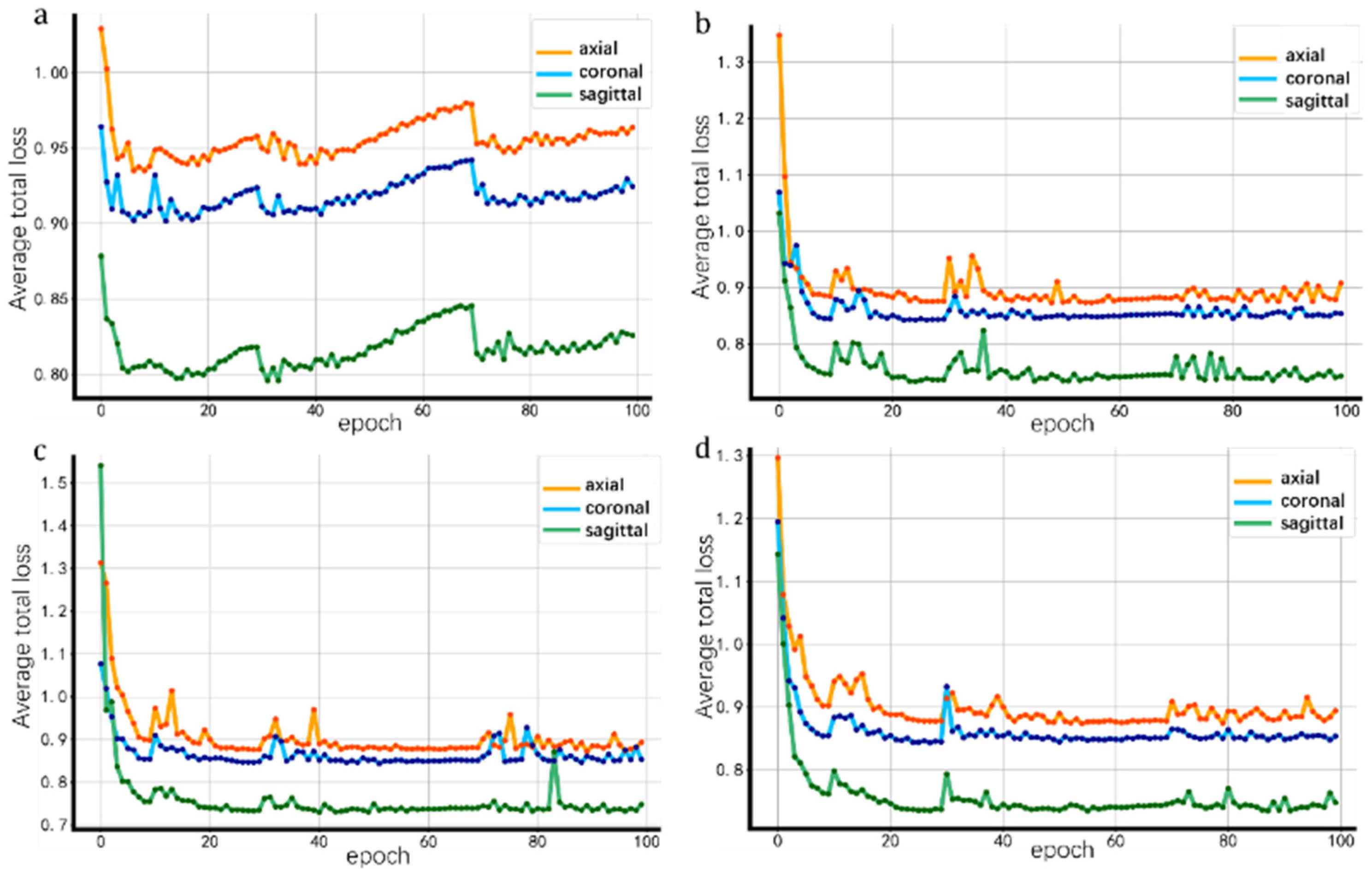
Figure 6 illustrates the trends of average total loss over training epochs across three anatomical planes (axial, coronal, and sagittal) under four model configurations, varying in the inclusion of ECA and CA modules. The model without either ECA or CA modules (Figure 6a) exhibits poor convergence during training, with large loss fluctuations and a noticeable increase after around 40 epochs, failing to achieve stable convergence. Models incorporating only one of the modules—either ECA or CA (Figure 6b,c)—begin to show some convergence around 20 epochs but still experience significant fluctuations later in training, with sharp loss spikes around epochs 30 and 70, indicating limited stability. In contrast, the model integrating both ECA and CA modules demonstrates faster convergence and greater stability throughout training. Its average total loss steadily decreases, remains low, and shows no significant fluctuations after convergence.

3.3. Segmentation Accuracy Results

3.3.1. Comparative Results from Different Methods

To evaluate segmentation accuracy, this study compares the proposed method against popular models, including U-Net [32], the improved QuickNAT, and FastSurfer, which is an optimized version built upon QuickNAT.

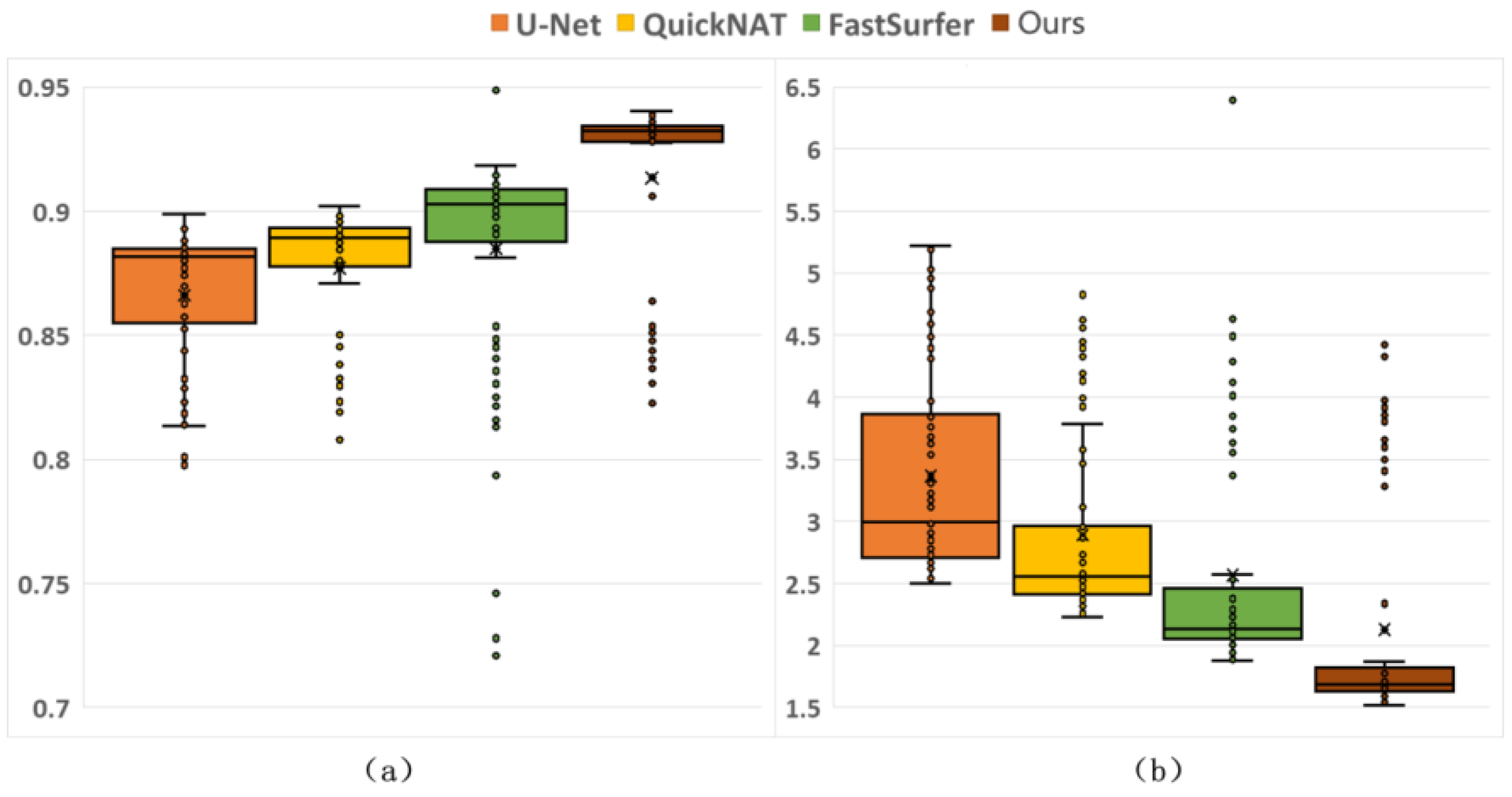
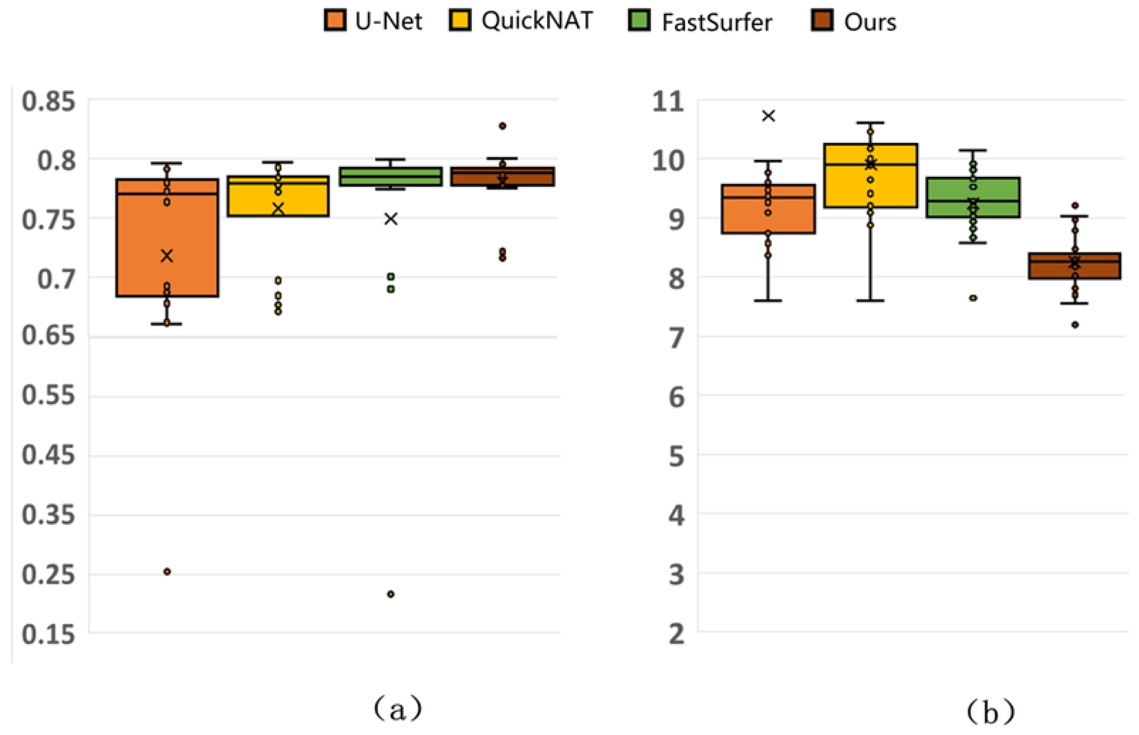
Figure 7 and Table 4 compare the performance of four methods—U-Net, QuickNAT, FastSurfer, and our proposed DRA-Net—based on the Dice coefficient and Hausdorff distance.

In terms of the Dice coefficient, our method achieves the highest mean scores(91.35), along with the highest median, showing the most concentrated data distribution and the fewest outliers, which indicates superior segmentation performance. While U-Net yields a lower average score (86.62), its performance is relatively stable, with few outliers, suggesting consistent segmentation results. In contrast, QuickNAT demonstrates less stability, and FastSurfer exhibits the highest variability, with a significant number of outliers.

Regarding the Hausdorff distance, our method again outperforms the others, achieving the lowest average distance (2.1279) and the most concentrated data distribution, reflecting minimal segmentation error. FastSurfer ranks second, with a mean distance of approximately 2.57, though with more scattered data. QuickNAT shows moderate performance, with an average of 2.8918, while U-Net performs the worst, exhibiting the highest mean and a more uniform data spread.

Table 4. Mean Dice coefficient and Hausdorff distance for different methods.

Method	Dice (%)	Hausdorff Distance (mm)
U-Net [32]	86.62 ± 2.81 *	3.3657 ± 0.8257 *
QuickNAT [25]	87.70 ± 2.67 *	2.8918 ± 0.7307 *
FastSurfer [27]	88.48 ± 4.38 *	2.5700 ± 0.8962 *
DRA-Net	91.35 ± 3.76	2.1279 ± 0.8888

Note. Boldface indicates the best results. * p < 0.05 based on the paired T-test between DRA-Net and other models.

Table 4. Mean Dice coefficient and Hausdorff distance for different methods.

Method	Dice (%)	Hausdorff Distance (mm)
U-Net [32]	86.62 ± 2.81 *	3.3657 ± 0.8257 *
QuickNAT [25]	87.70 ± 2.67 *	2.8918 ± 0.7307 *
FastSurfer [27]	88.48 ± 4.38 *	2.5700 ± 0.8962 *
DRA-Net	91.35 ± 3.76	2.1279 ± 0.8888

Note. Boldface indicates the best results. * p < 0.05 based on the paired T-test between DRA-Net and other models.

3.3.2. Generalization Results

To further validate the generalization capability of the proposed model, the 20 subjects from the OASIS-TRT-20 dataset were used as an independent test set. As shown in Figure 8, the method achieves the best performance on both the Dice coefficient and Hausdorff distance, demonstrating high segmentation accuracy and strong stability.

3.3.3. Comparison with Mainstream Methods

To objectively and comprehensively evaluate the generalization capability of different image segmentation models on the same independent test set, this study selected a variety of representative methods, including both traditional neuroimaging analysis tools and advanced deep learning-based architectures. A detailed comparison was conducted to assess the performance of each technique on the segmentation task and to verify the effectiveness of the proposed model, as summarized in Table 5.

As shown in Table 5, the proposed DRA-Net model outperforms all other compared methods in terms of segmentation performance, achieving the highest average Dice coefficient of 77.99%. In addition, DRA-Net obtained the best result on the average Hausdorff distance (8.2571), indicating superior consistency in capturing the true anatomical boundaries.

Specifically, the SLANT-27 FT model, which is based on a Transformer [33], ranked second in performance, surpassing the traditional CNN-based U-Net model. This advantage may stem from the Transformer’s capability to model long-range dependencies more effectively. It is also noteworthy that the basic version of the F-CNN [34] method yielded the poorest performance; however, after incorporating a multi-view feature fusion strategy and adopting an improved QuickNAT architecture, its segmentation accuracy significantly improved from 57.9% to 75.84%, reaching a level comparable to that of SLANT-27 FT [35].

Table 5. Dice coefficients of various models on the OASIS-TRT-20 dataset.

Method		Dice (%)	Hausdorff Distance (mm)
U-Net [32]	CNN	71.83 ± 12.88	10.728 ± 7.1801
QuickNAT [25]	CNN	75.84 ± 4.42	9.8983 ± 1.3562
FastSurfer [27]	CNN	74.92 ± 12.01	9.2437 ± 0.5632
FreeSurfer [20]	Atlas-based	74.75 ± 5.83	8.9852 ± 0.4936
FSL [14]	Atlas-based	64.3 ± 0.29	—
JLF [36]	Atlas-based	74.6 ± 0.90	—
F-CNN [34]	CNN	57.9 ± 0.24	—
Naive U-Net [37]	CNN	60.6 ± 0.60	—
SLANT-8 [35]	Transformer	69.9 ± 1.40	—
SLANT-27 [35]	Transformer	76.6 ± 0.80	—
SLANT-27 FT [35]	Transformer	75.9 ± 1.70	—
DRA-Net	CNN	77.99 ± 2.83	8.2571 ± 0.5009

Note. Boldface indicates the best results.

Table 5. Dice coefficients of various models on the OASIS-TRT-20 dataset.

Method		Dice (%)	Hausdorff Distance (mm)
U-Net [32]	CNN	71.83 ± 12.88	10.728 ± 7.1801
QuickNAT [25]	CNN	75.84 ± 4.42	9.8983 ± 1.3562
FastSurfer [27]	CNN	74.92 ± 12.01	9.2437 ± 0.5632
FreeSurfer [20]	Atlas-based	74.75 ± 5.83	8.9852 ± 0.4936
FSL [14]	Atlas-based	64.3 ± 0.29	—
JLF [36]	Atlas-based	74.6 ± 0.90	—
F-CNN [34]	CNN	57.9 ± 0.24	—
Naive U-Net [37]	CNN	60.6 ± 0.60	—
SLANT-8 [35]	Transformer	69.9 ± 1.40	—
SLANT-27 [35]	Transformer	76.6 ± 0.80	—
SLANT-27 FT [35]	Transformer	75.9 ± 1.70	—
DRA-Net	CNN	77.99 ± 2.83	8.2571 ± 0.5009

Note. Boldface indicates the best results.

3.4. Cortical Structure Segmentation Results

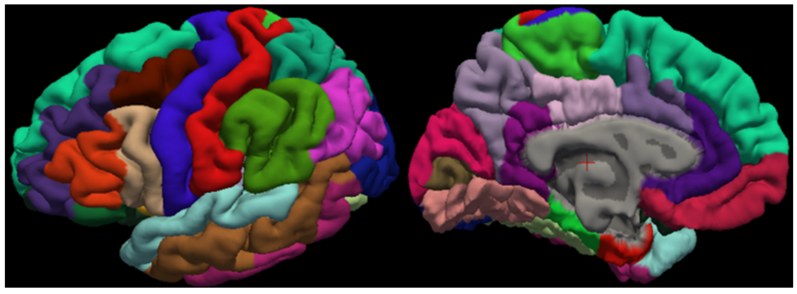
The cortical segmentation results obtained in this study are presented in Figure 9 and Figure 10.

Figure 9 and Figure 10 illustrate the high accuracy and excellent cortical conformity of the segmentation results produced by the DRA-Net model, accurately reconstructing both the outer surface and the inner (white matter) surface of the human cerebral cortex. This precise segmentation not only captures the overall cortical contours but also accurately delineates the boundaries of cortical subregions, reflecting the natural anatomy of the brain’s gyri and sulci.

Table 6. Quantitative results of multiple ROIs using DRA_Net.

ROI	Dice (%)	Hausdorff Distance (mm)	ROI	Dice (%)	Hausdorff Distance (mm)
Insula	87.64 ± 3.40	4.7818 ± 1.6534	Posterior cingulate	78.83 ± 5.43	6.7194 ± 2.1258
Superior frontal	84.72 ± 4.16	13.4316 ± 3.0392	Postcentral	78.76 ± 6.21	12.6653 ± 3.5746
Precentral	84.62 ± 4.31	9.5087 ± 1.0761	Inferior temporal	78.71 ± 3.50	10.5309 ± 4.2501
Superior temporal	83.50 ± 4.03	12.6089 ± 5.8031	Middle frontal	77.56 ± 4.78	11.8840 ± 2.4110
Precuneus	83.00 ± 3.56	8.9933 ± 2.6247	Fusiform	76.43 ± 4.88	10.7908 ± 3.2435
Middle temporal	81.27 ± 4.71	11.8217 ± 3.5855	Orbitofrontal	75.01 ± 3.84	9.1331 ± 1.0612
Parietal	79.67 ± 4.83	11.6662 ± 1.9720	Anterior cingulate	74.78 ± 5.42	7.2973 ± 2.2701
Paracentral	79.58 ± 4.25	9.0082 ± 2.7561	Cuneus	74.74 ± 4.72	9.7077 ± 2.4501
Lingual	79.57 ± 4.70	7.5641 ± 2.4250	Inferior frontal	71.79 ± 6.32	9.9689 ± 2.2038
Parahippocampal	79.29 ± 5.90	4.2071 ± 1.2654	Entorhinal	68.46 ± 6.65	6.1400 ± 1.0972

Note: we selected several representative regions and merged them into the 20 ROIs listed above.

shows that there are differences in the Dice coefficients among different brain regions. Among them, the insula has the highest Dice coefficient, while the entorhinal cortex has the lowest Dice coefficient. This result may be related to the structural characteristics of each brain region, and it may also be related to the accuracy of training data annotation.

4. Discussion

4.1. Advantages of the Proposed Method

This study demonstrates that DRA-Net significantly outperforms mainstream methods such as U-Net, QuickNAT, and FastSurfer in terms of segmentation accuracy and training stability. Furthermore, the model exhibits high robustness and generalization ability when faced with untrained datasets, enabling it to stably perform segmentation tasks across different data and anatomical structures. Even when dealing with completely new, independent test data, the model can achieve effective inference based on learned semantic features, demonstrating precise recognition ability for the brain cortex.

The model effectively differentiates between various cortical areas during segmentation, maintaining the anatomical coherence of each cortical subregion and showcasing strong spatial awareness. When handling the brain cortex’s complex folds, the segmentation aligns closely with the true cortical folding contours, evidencing the model’s outstanding performance in capturing fine structural details. This highlights not only precise global structural localization but also efficient identification of subtle local anatomical features. This result is attributed to the multi-scale context information fusion strategy introduced deeply into the DRA-Net network structure, which enables the model to effectively cope with complex situations.

4.2. Analysis of DRB and RAB

In this study, we use the combination of DRB and RAB modules, improving segmentation accuracy and generalization. Specifically, the DRB directly acts on the original input image, aiming to dynamically enhance key feature channels through efficient interaction between channels, thereby improving the accuracy of feature extraction and the sensitivity of the model to local information. The RAB acts on image features, focusing on capturing spatial contextual information, establishing local and global spatial dependencies through multi-dimensional pooling and directional weighting calibration, thereby enhancing spatial perception capabilities. The conventional dual-attention mechanisms [38,39] often rely on fully connected layers for dimensionality reduction and global 2D spatial weight learning. In contrast, the proposed DRB uses a lightweight 1D convolution to achieve full-channel information interaction without dimension reduction, combined with Maxout for dynamic weight optimization, enhancing the contribution of key feature channels through ECA. Compared with traditional 2D spatial attention [40], ECA combined with 1D spatial pooling has lower computational complexity and fewer parameters, significantly reducing computational overhead while maintaining feature representation capability. Moreover, ECA dynamically adjusts the importance of different channels through local cross-channel interactions, while 1D spatial pooling captures both global and local information along the two (height and width) directions, making the model more robust to noise. Meanwhile, through CA, the RAB captures multi-dimensional global and local information via directional pooling and compression along both the height and width dimensions, introduces directional feature weights for recalibration, and establishes spatial correlations among features. Therefore, the DRB and RAB allow the model to improve segmentation accuracy and generalization by highlighting the useful features and suppressing useless features.

4.3. Analysis of Segmentation Performance

We evaluated the segmentation performance of the key ROIs on the OASIS-TRT-20 test set (Table 6) to provide a detailed assessment of the model’s applicability across different brain regions. This analysis not only identifies ROIs where the model achieves satisfactory accuracy but also highlights regions with lower performance, thereby indicating areas that may benefit from further methodological refinement in future work. Additionally, due to the complex folding structure of the cerebral cortex and the often unclear intensity contrast between regions, the model is more prone to deviations or discontinuities when handling fine boundaries of sulci and gyri. Such errors may have little impact on overall voxel overlap, but they are more apparent in boundary evaluation metrics (e.g., Hausdorff distance), especially in regions with broad boundaries (such as the frontal gyrus, temporal gyrus and Parietal gyrus), where boundary inaccuracies are more likely to accumulate into significant local deviations.

4.4. Limitation

The proposed DRA-Net demonstrates strong robustness and generalization across multiple datasets, but several limitations of this study should be noted. First, the current loss used a fixed 1:1 weighting scheme during training, without systematically analyzing the sensitivity of the weighting parameters α and β. Moreover, this loss may not be optimal for the volume imbalance among various brain regions (e.g., small structures such as the insula vs. large regions such as the frontal lobe). Therefore, future work may consider adaptive or data-driven loss weighting methods. Second, this study utilized an automated annotation approach based on the DKT atlas for model training. This strategy can ensure the consistency and reproducibility of training samples, but it may introduce certain biases, such as insufficient sensitivity to individual structural variations and limited accuracy in regions with complex cortical boundaries. Future work could mitigate these biases by integrating multi-atlas information or incorporating manual label refinement. Thirdly, the proposed network learns the anatomical representations of brain structures based on the 2D slice orientation, which could result in potential loss compared to 3D models. In future work, exploration-based full 3D models will be evaluated.

5. Conclusions

This paper presents DRA-Net, an intelligent cortical segmentation model designed to enhance the accuracy of brain cortex region segmentation in medical image analysis while maintaining high computational efficiency. This study demonstrates that, based on a U-shaped architecture, integrating the Dynamic Recalibration Block (DRB) and the Region-Aware Block (RAB) effectively balances computational efficiency, model stability, and segmentation accuracy. This approach offers promising technical support for applications such as the localization of disease-related brain targets and surgical navigation.

References

1. Yang, J.; Sui, S.F.; Liu, Z. Brain structure and structural basis of neurodegenerative diseases. Biophys. Rep. 2022, 8, 170–181. [Google Scholar] [CrossRef] [PubMed]
2. Carew, T.J.; Magsamen, S.H. Neuroscience and Education: An Ideal Partnership for Producing Evidence-Based Solutions to Guide 21st Century Learning. Neuron 2010, 67, 685–688. [Google Scholar] [CrossRef] [PubMed]
3. DeYoe, E.A.; Bandettini, P.; Neitz, J.; Miller, D.; Winans, P. Functional magnetic resonance imaging (FMRI) of the human brain. J. Neurosci. Methods 1994, 54, 171–187. [Google Scholar] [CrossRef]
4. Sajjanar, R.; Dixit, U.D. Advanced Fusion of 3D U-Net-LSTM Models for Accurate Brain Tumor Segmentation. Int. J. Adv. Comput. Sci. Appl. 2024, 15, 488–502. [Google Scholar] [CrossRef]
5. Siraisi, N.G. Vesalius and Human Diversity in De humani corporis fabrica. J. Warbg. Court. Inst. 1994, 57, 60–88. [Google Scholar] [CrossRef]
6. Yang, P.; Zhang, R.; Hu, C.; Guo, B. GMDNet: Grouped Encoder-Mixer-Decoder Architecture Based on the Role of Modalities for Brain Tumor MRI Image Segmentation. Electronics 2025, 14, 1658. [Google Scholar] [CrossRef]
7. Damiani, D.; Nascimento, A.M.; Pereira, L.K. Cortical brain functions–the brodmann legacy in the 21st century. Arq. Bras. De. Neurocir. Braz. Neurosurg. 2020, 39, 261–270. [Google Scholar] [CrossRef]
8. Sporns, O.; Tononi, G.; Kötter, R. The human connectome: A structural description of the human brain. PLoS Comput. Biol. 2005, 1, e42. [Google Scholar] [CrossRef] [PubMed]
9. Ajita, R. Galen and his contribution to anatomy: A review. J. Evol. Med. Dent. Sci. 2015, 4, 4509–4517. [Google Scholar] [CrossRef]
10. Loukas, M.; Pennell, C.; Groat, C.; Tubbs, R.S.; Cohen-Gadol, A.A. Korbinian Brodmann (1868–1918) and his contributions to mapping the cerebral cortex. Neurosurgery 2011, 68, 6–11. [Google Scholar] [CrossRef]
11. Lancaster, J.L.; Woldorff, M.G.; Parsons, L.M.; Liotti, M.; Freitas, C.S.; Rainey, L.; Kochunov, P.V.; Nickerson, D.; Mikiten, S.A.; Fox, P.T. Automated Talairach atlas labels for functional brain mapping. Hum. Brain Mapp. 2000, 10, 120–131. [Google Scholar] [CrossRef] [PubMed]
12. Fang, A.; Nowinski, W.L.; Nguyen, B.T.; Bryan, R.N. Three-dimensional Talairach-Tournoux brain atlas. In Proceedings of the Medical Imaging 1995: Image Display, San Diego, CA, USA, 26–28 February 1995; pp. 583–592. [Google Scholar]
13. Friston, K.J. Statistical parametric mapping. In Neuroscience Databases: A Practical Guide; Springer: Boston, MA, USA, 2003; pp. 237–250. [Google Scholar]
14. Jenkinson, M.; Beckmann, C.F.; Behrens, T.E.; Woolrich, M.W.; Smith, S.M. Fsl. Neuroimage 2012, 62, 782–790. [Google Scholar] [CrossRef] [PubMed]
15. Cox, R.W. AFNI: Software for analysis and visualization of functional magnetic resonance neuroimages. Comput. Biomed. Res. 1996, 29, 162–173. [Google Scholar] [CrossRef] [PubMed]
16. Aboudi, F.; Drissi, C.; Kraiem, T. A Hybrid Model for Ischemic Stroke Brain Segmentation from MRI Images using CBAM and ResNet50-UNet. Int. J. Adv. Comput. Sci. Appl. 2024, 15, 950–962. [Google Scholar] [CrossRef]
17. Tzourio-Mazoyer, N.; Landeau, B.; Papathanassiou, D.; Crivello, F.; Etard, O.; Delcroix, N.; Mazoyer, B.; Joliot, M. Automated anatomical labeling of activations in SPM using a macroscopic anatomical parcellation of the MNI MRI single-subject brain. Neuroimage 2002, 15, 273–289. [Google Scholar] [CrossRef] [PubMed]
18. Li, X.; Morgan, P.S.; Ashburner, J.; Smith, J.; Rorden, C. The first step for neuroimaging data analysis: DICOM to NIfTI conversion. J. Neurosci. Methods 2016, 264, 47–56. [Google Scholar] [CrossRef] [PubMed]
19. Desikan, R.S.; Ségonne, F.; Fischl, B.; Quinn, B.T.; Dickerson, B.C.; Blacker, D.; Buckner, R.L.; Dale, A.M.; Maguire, R.P.; Hyman, B.T. An automated labeling system for subdividing the human cerebral cortex on MRI scans into gyral based regions of interest. Neuroimage 2006, 31, 968–980. [Google Scholar] [CrossRef] [PubMed]
20. Fischl, B. FreeSurfer. Neuroimage 2012, 62, 774–781. [Google Scholar] [CrossRef]
21. Dahnke, R.; Yotter, R.A.; Gaser, C. Cortical thickness and central surface estimation. Neuroimage 2013, 65, 336–348. [Google Scholar] [CrossRef]
22. Destrieux, C.; Fischl, B.; Dale, A.; Halgren, E. Automatic parcellation of human cortical gyri and sulci using standard anatomical nomenclature. Neuroimage 2010, 53, 1–15. [Google Scholar] [CrossRef]
23. Mehta, R.; Majumdar, A.; Sivaswamy, J. BrainSegNet: A convolutional neural network architecture for automated segmentation of human brain structures. J. Med. Imaging 2017, 4, 024003. [Google Scholar] [CrossRef]
24. Wachinger, C.; Reuter, M.; Klein, T. DeepNAT: Deep convolutional neural network for segmenting neuroanatomy. NeuroImage 2018, 170, 434–445. [Google Scholar] [CrossRef] [PubMed]
25. Roy, A.G.; Conjeti, S.; Navab, N.; Wachinger, C.; Initiative, A.s.D.N. QuickNAT: A fully convolutional network for quick and accurate segmentation of neuroanatomy. NeuroImage 2019, 186, 713–727. [Google Scholar] [CrossRef]
26. Coupé, P.; Mansencal, B.; Clément, M.; Giraud, R.; de Senneville, B.D.; Ta, V.-T.; Lepetit, V.; Manjon, J.V. AssemblyNet: A large ensemble of CNNs for 3D whole brain MRI segmentation. NeuroImage 2020, 219, 117026. [Google Scholar] [CrossRef] [PubMed]
27. Henschel, L.; Conjeti, S.; Estrada, S.; Diers, K.; Fischl, B.; Reuter, M. Fastsurfer-a fast and accurate deep learning based neuroimaging pipeline. NeuroImage 2020, 219, 117012. [Google Scholar] [CrossRef] [PubMed]
28. Klein, A.; Tourville, J. 101 labeled brain images and a consistent human cortical labeling protocol. Front. Neurosci. 2012, 6, 171. [Google Scholar] [CrossRef] [PubMed]
29. Wang, Q.; Wu, B.; Zhu, P.; Li, P.; Zuo, W.; Hu, Q. ECA-Net: Efficient channel attention for deep convolutional neural networks. In Proceedings of the IEEE/CVF Conference on Computer Vision and Pattern Recognition, Seattle, WA, USA, 13–19 June 2020; pp. 11534–11542. [Google Scholar]
30. Goodfellow, I.; Warde-Farley, D.; Mirza, M.; Courville, A.; Bengio, Y. Maxout networks. In Proceedings of the International Conference on Machine Learning, Atlanta, GA, USA, 17–19 June 2013; pp. 1319–1327. [Google Scholar]
31. Choi, M.; Kim, H.; Han, B.; Xu, N.; Lee, K.M. Channel attention is all you need for video frame interpolation. In Proceedings of the AAAI Conference on Artificial Intelligence, New York, NY, USA, 7–12 February 2020; pp. 10663–10671. [Google Scholar]
32. Ronneberger, O.; Fischer, P.; Brox, T. U-net: Convolutional networks for biomedical image segmentation. In Proceedings of the Medical Image Computing and Computer-Assisted Intervention–MICCAI 2015: 18th International Conference, Munich, Germany, 5–9 October 2015; pp. 234–241. [Google Scholar]
33. Vaswani, A.; Shazeer, N.; Parmar, N.; Uszkoreit, J.; Jones, L.; Gomez, A.N.; Kaiser, Ł.; Polosukhin, I. Attention is all you need. Adv. Neural Inf. Process. Syst. 2017, 5998–6008. [Google Scholar]
34. Zhao, W.; Fu, H.; Luk, W.; Yu, T.; Wang, S.; Feng, B.; Ma, Y.; Yang, G. F-CNN: An FPGA-based framework for training convolutional neural networks. In Proceedings of the 2016 IEEE 27Th International Conference on Application-Specific Systems, Architectures and Processors (ASAP), London, UK, 6–8 July 2016; pp. 107–114. [Google Scholar]
35. Huo, Y.; Xu, Z.; Aboud, K.; Parvathaneni, P.; Bao, S.; Bermudez, C.; Resnick, S.M.; Cutting, L.E.; Landman, B.A. Spatially localized atlas network tiles enables 3D whole brain segmentation from limited data. In Proceedings of the Medical Image Computing and Computer Assisted Intervention–MICCAI 2018: 21st International Conference, Granada, Spain, 16–20 September 2018; pp. 698–705. [Google Scholar]
36. Wang, H.; Yushkevich, P.A. Multi-atlas segmentation with joint label fusion and corrective learning—An open source implementation. Front. Neuroinform. 2013, 7, 27. [Google Scholar] [CrossRef] [PubMed]
37. Çiçek, Ö.; Abdulkadir, A.; Lienkamp, S.S.; Brox, T.; Ronneberger, O. 3D U-Net: Learning dense volumetric segmentation from sparse annotation. In Proceedings of the Medical Image Computing and Computer-Assisted Intervention–MICCAI 2016: 19th International Conference, Athens, Greece, 17–21 October 2016; pp. 424–432. [Google Scholar]
38. Khedir, M.; Amara, K.; Dif, N.; Kerdjidj, O.; Atalla, S.; Ramzan, N. BrainAR: Automated Brain Tumor Diagnosis with Deep Learning and 3D Augmented Reality Visualization. IEEE Access 2025, 13, 128639–128653. [Google Scholar] [CrossRef]
39. Fu, J.; Liu, J.; Tian, H.; Li, Y.; Bao, Y.; Fang, Z.; Lu, H. Dual attention network for scene segmentation. In Proceedings of the IEEE/CVF Conference on Computer Vision and Pattern Recognition, Long Beach, CA, USA, 15–20 June 2019; pp. 3146–3154. [Google Scholar]
40. Hayat, M.; Aramvith, S.; Bhattacharjee, S.; Ahmad, N. Attention ghostunet++: Enhanced segmentation of adipose tissue and liver in ct images. arXiv 2025, arXiv:2504.11491. [Google Scholar]
Figure 1. Preprocessing steps.
Electronics 14 03631 g001
Figure 2. Network architecture diagram.
Electronics 14 03631 g002
Figure 3. Structure of the Dynamic Recalibration Block (DRB).
Electronics 14 03631 g003
Figure 4. Structure of the Region-Aware Block (RAB).
Electronics 14 03631 g004
Figure 5. Average training loss metrics of the proposed model.
Electronics 14 03631 g005
Figure 6. Ablation study results on average loss parameters. (a) without ECA and CA; (b) without CA; (c) without ECA; (d) with ECA and CA.
Electronics 14 03631 g006
Figure 7. The segmentation performance scores across different models: (a) Dice coefficient; (b) Hausdorff distance. In the boxplots, the “.” indicate outliers, and the “×” represents the mean value.
Electronics 14 03631 g007
Figure 8. Generalization performance comparison across datasets. (a) Average Dice coefficient; (b) average Hausdorff distance. In the boxplots, the “.” indicate outliers, and the “×” represents the mean value.
Electronics 14 03631 g008
Figure 9. An example illustrating the structural segmentation results of the cerebral cortex. Different colors are used only for visualization purposes to distinguish segmented regions, without specific anatomical meaning.
Electronics 14 03631 g009
Figure 10. An example of the segmentation results for the outer surface of the cerebral cortex. Different colors are used only for visualization purposes to distinguish segmented regions, without specific anatomical meaning.
Electronics 14 03631 g010