Expensive Highly Constrained Antenna Design Using Surrogate-Assisted Evolutionary Optimization

Abstract

Antenna structure design constitutes a computationally expensive optimization problem due to the requirement for full-wave electromagnetic (EM) simulations. Surrogate-assisted evolutionary algorithms offer a promising approach for addressing such challenges. However, several challenges remain in solving expensive, highly constrained antenna design problems. This paper introduces a surrogate-assisted dynamic constrained multi-objective evolutionary algorithm framework to tackle expensive and highly constrained antenna design optimization tasks. A multi-layer perceptron (MLP) is employed as the surrogate model to approximate EM evaluations and alleviate the computational burden, while a dynamic scale-constrained boundary strategy is implemented to handle highly constraints. The effectiveness of the proposed method is validated on a set of constrained benchmark problems and two antenna design cases.

1. Introduction

Antennas are fundamental elements in wireless communication systems, playing a pivotal role in radiation and reception performance, thereby directly influencing link quality, data rate, and system capacity [1,2]. Antenna structure design is commonly formulated as an optimization problem and has attracted significant research attention. Existing approaches are broadly classified into two categories: (1) Numerical optimization methods leverage mathematical optimization ideas, and have been successfully applied to antenna structure design, e.g., gradient-based method [3], quasi-newton method [4], and convex relaxation [5]. However, there are some challenges in the mathematical method for solving complex antenna design, such as the optimization problem being nonlinear, non-differentiable, and multi-model. Therefore, (2) nature-inspired methods, particularly evolutionary algorithms (EAs), have consequently gained significant traction for overcoming these limitations. EAs are increasingly applied in antenna design; for example, particle swarm optimization (PSO) was used to drive the design variables of antenna optimization problems [6], differential evolution (DE) was used to optimize the structure of antenna with complex requirements [7], and a multi-objective optimization method with genetic algorithm was used to design antenna array [8].

However, evolutionary algorithms (EAs) typically require numerous evaluations to obtain satisfactory solutions for antenna design. This process is computationally expensive since full-wave electromagnetic (EM) simulations, the standard method for evaluating antenna performance, are highly resource-intensive. Consequently, antenna design optimization represents a class of computationally expensive optimization problems. To address this challenge, surrogate-assisted evolutionary algorithms (SAEAs) have been developed, leveraging surrogate models (also known as soft computing techniques) to approximate the computationally prohibitive EM evaluations [9]. By significantly reducing the number of exact (high-fidelity) function evaluations required, SAEAs dramatically lower the computational cost. These methods have been successfully applied across diverse engineering domains, including dynamic flexible job shop scheduling [10], blast furnace optimization [11], and crude oil distillation unit design [12]. Surrogate models are also employed in eddy current testing for the estimation and classification of structural delaminations [13,14].

In addition, SAEAs have also been employed in antenna design to alleviate the computational burden of electromagnetic simulations. For instance, a circular antenna array was designed using surrogate-assisted differential evolution [15]; a substrate-integrated waveguide (SIW) cavity-backed slot antenna was designed using surrogate-assisted particle swarm optimization [16]; a Yagi–Uda antenna was designed using a surrogate-assisted approach [17]; and a multi-band antenna was designed using surrogate-assisted MOEA/D [18].

However, effectively solving antenna design optimization problems involving complex engineering constraints remains challenging. The constrained antenna design problems have been solved in refs. [19,20], but high EM simulation cost was involved. Although the expensive constrained antenna design problems have also been studied in ref. [21], there are no highly constraints in these antenna problems, and the proposed algorithms cannot solve the antenna problems with highly constraints. As evidenced by the aforementioned studies, research on solving computationally expensive and highly constrained antenna design optimization problems remains scarce. In practice, numerous complex antenna design tasks often entail such optimization problems, characterized by costly full-wave EM and stringent constraints. To address this challenge, this paper proposes a surrogate-assisted evolutionary optimization framework. Specifically, a multi-layer perceptron (MLP) is employed to approximate the computationally expensive EM simulations, alleviating the associated computational burden. Concurrently, a dynamic scale-constrained boundary strategy is introduced to effectively handle the stringent constraints. The main contributions of this work include the following:

1.

A framework with a surrogate-assisted dynamic constrained multi-objective evolutionary algorithm is proposed to solve the expensive and highly constrained antenna problems.

2.

A multi-layer perception is used to approximate EM evaluation to overcome the difficulty of high costs, and a dynamic scale-constrained boundary strategy is used to solve the issue of highly constraints.

3.

Some numerical studies are carried out to verify the effectiveness of our method. The superior performance is confirmed not only for complex benchmark problems, but also for antenna examples in wideband antenna and microstrip antenna designs.

The rest of this paper is organized as follows. Section 2 provides preliminary information about constrained optimization techniques and multi-layer perception networks. Section 3 establishes our proposed framework and describes details of the proposed method. Thereafter, Section 4 presents numerical case studies of this framework in benchmark problems and two antenna design optimization problems. Finally, Section 5 summarizes the paper and points to directions for future research.

2. Basic Techniques

2.1. Constrained Optimization Techniques

In the constrained optimization problem (COP), constrained handle techniques are a vital component and have garnered increasing interest in recent years. These techniques can be divided into four categories [22]: the penalty function method [23], the objective and constraint separately handle method [24], the ensemble method [25], and the multi-objective method [26]. In these methods, the multi-objective method is popular in solving COP and has been widely studied for decades. A dynamic constrained handle method was proposed to solve COP in ref. [27], where a COP is converted into an equivalent dynamic constrained multi-objective optimization problem (DCMOP) with three objectives: the original objective, a constraint-violation objective, and a niche-count objective. This method will be used in this paper. The details of this method are as follows. A COP comprises an objective function and m constraint functions. The mathematical formulation is shown as follows:

$$\begin{array}{c}\hfill \begin{array}{cc}min\hfill & \mathit{F}\left(\mathit{x}\right)=f\left(\mathit{x}\right)\hfill \\ st:\hfill & \mathit{g}\left(\mathit{x}\right)=(g_1\left(\mathit{x}\right),g_2\left(\mathit{x}\right),\dots ,g_m\left(\mathit{x}\right))\le \mathbf{0}\hfill \\ where\hfill & \mathit{x}=(x_1,x_2,\dots ,x_D)\in \mathit{X}\hfill \\ & \mathit{X}=\left\{\mathit{x}\right|\mathit{l}\le \mathit{x}\le \mathit{u}\}\hfill \\ & \mathit{l}=(l_1,l_2,\dots ,l_D),\mathit{u}=(u_1,u_2,\dots ,u_D),\hfill \end{array}\end{array}$$

(1)

where $f\left(\mathit{x}\right)$ is the objective function; $\mathit{g}\left(\mathit{x}\right)$ is the constraint function; $\mathbf{0}$ is the constrained boundary; $\mathit{x}$ is the decision variable; $\mathit{X}$ is decision space; $\mathit{l}$ and $\mathit{u}$ are lower and upper ranges of decision variable, respectively; and D is the dimension of the decision variable. To handle the COP, the COP is constructed as a multi-objective optimization problem:

$$\begin{array}{c}\hfill \begin{array}{cc}min\hfill & \mathit{F}\left(\mathit{x}\right)=\left(f\right(\mathit{x}),cv(\mathit{x}),nc(\mathit{x}|\mathit{U},\sigma ))\hfill \\ st:\hfill & \mathit{g}\left(\mathit{x}\right)\le \mathbf{0},\hfill \end{array}\end{array}$$

(2)

where $cv\left(\mathit{x}\right)$ is the violation function, which is the average of the degree of violation constraints for an individual. $nc\left(\mathit{x}\right|\mathit{U},\sigma )$ is niche count function, which is used to measure the crowded degree of an individual; $\mathit{U}$ is the set of current parent and offspring populations; and $\sigma$ is the niche radius:

$$\begin{array}{c}\hfill nc\left(\mathit{x}\right|\mathit{U},\sigma )=\sum _{i=1,{\mathit{x}}_{\mathit{i}}\ne \mathit{x}}^{L}sh(\mathit{x},{\mathit{x}}_{\mathit{i}}),\end{array}$$

(3)

where $sh(\mathit{x},{\mathit{x}}_{\mathit{i}})$ is the sharing function between two solutions ${\mathit{x}}_{\mathbf{1}}$ and ${\mathit{x}}_{\mathbf{2}}$, which is defined as follows with a niche:

$$\begin{array}{c}\hfill sh(\mathit{x},{\mathit{x}}_{\mathit{i}})=\left\{\begin{array}{cc}1-\left({\displaystyle \frac{d({\mathit{x}}_{\mathbf{1}},{\mathit{x}}_{\mathbf{2}})}{\sigma }}\right),\hfill & \mathrm{i}\mathrm{f} d({\mathit{x}}_{\mathbf{1}},{\mathit{x}}_{\mathbf{2}})\le \sigma \hfill \\ 0,\hfill & \mathrm{o}\mathrm{t}\mathrm{h}\mathrm{e}\mathrm{r}\mathrm{w}\mathrm{i}\mathrm{s}\mathrm{e}.\hfill \end{array}\right.\end{array}$$

(4)

Apparently, (2) is not equivalent to (1). Furthermore, it is also challenging to handle high constraints using the multi-objective method for (2). To address these issues, a DCMOP is proposed:

$$\begin{array}{c}\hfill \begin{array}{cc}min\hfill & \mathit{F}\left(\mathit{x}\right)=\left(f\right(\mathit{x}),cv(\mathit{x}),nc(\mathit{x}|\mathit{U},\sigma ))\hfill \\ st:\hfill & \mathit{g}\left(\mathit{x}\right)\le {\mathit{\epsilon }}^{\mathit{s}},\hfill \end{array}\end{array}$$

(5)

where ${\mathit{\epsilon }}^{\mathit{s}}=({\epsilon }_1^s,{\epsilon }_2^s,\cdots ,{\epsilon }_q^s),s=0,1,\cdots ,S$, and ${\mathit{\epsilon }}^{\mathbf{0}}>{\mathit{\epsilon }}^{\mathbf{0}}>\cdots >{\mathit{\epsilon }}^{\mathit{S}}=\mathbf{0}$, ${\mathit{\epsilon }}^{\mathit{s}}$ is the dynamic constrained boundary, s is the environment state, S is the maximum environment state; ${\sigma }^0>{\sigma }^1>\cdots ,{\sigma }^S$, ${\sigma }^s$ is a dynamic niche radius. From (5), when $s=S$, ${\mathit{\epsilon }}^{\mathit{S}}=\mathbf{0}$, ${\sigma }^S=0$, this case means that $cv\left(\mathit{x}\right)=0$ and $nc\left(\mathit{x}\right|\mathit{U},\sigma )=0$. Thus, the DCMOP is

$$\begin{array}{c}\hfill \begin{array}{cc}min\hfill & \mathit{F}\left(\mathit{x}\right)=\left(f\right(\mathit{x}),0,0)\hfill \\ st:\hfill & \mathit{g}\left(\mathit{x}\right)\le \mathbf{0}.\hfill \end{array}\end{array}$$

(6)

Therefore, when $s=S$, the DCMOP is equivalent to COP. Initially, the dynamic constraint boundary ${\mathit{\epsilon }}^{\mathit{s}}$ is set to a sufficiently large value to ensure that all individuals in the initial population are feasible. Then the boundary decreases as the environment state increases. Likewise, the dynamic niche radius ${\sigma }^s$ also decreases as the environment state increases.

2.2. Multi-Layer Perception Neural Network

In ANNs, the MLP as a multi-layered feed-forward neural network has been widely used for regression and classification based on the discovery of practical experience. In this paper, an MLP regressor comprising L fully connected hidden layers is used. Each hidden neuron employs the Sigmoid activation function $\sigma (·)$ to introduce nonlinearity. The MLP formulation is

$$\begin{array}{c}\hfill \widehat{y}={\mathit{W}}^{\left(\mathrm{out}\right)}{\mathit{h}}^{\left(L\right)}+b^{\left(\mathrm{out}\right)},\end{array}$$

(7)

where ${\mathit{h}}^{\left(k\right)},k=1,2,\cdots ,L$ is the output of hidden layer:

$$\begin{array}{c}\hfill {\mathit{h}}^{\left(k\right)}=\sigma ({\mathit{W}}^{\left(k\right)}{\mathit{h}}^{(k-1)}+{\mathit{b}}^{\left(k\right)}),k=1,2,\cdots ,L,\end{array}$$

(8)

where ${{\mathit{W}}^{\left(k\right)},{\mathit{b}}^{\left(k\right)}}_{k=1}^L$ and ${\mathit{W}}^{\left(\mathrm{out}\right)},b^{\left(\mathrm{out}\right)}$ are the parameters to be learned, and $\sigma$ is the Sigmoid activation function in this paper.

3. Method

3.1. Algorithm Framework

As Section 1 mentioned, this paper proposes a framework with a surrogate-assisted dynamic constrained multi-objective evolutionary algorithm to solve expensive and highly constrained optimization problems. The framework is shown in Algorithm 1.

Algorithm 1 The pseudo-code of the surrogate-assisted dynamic constrained multi-objective evolutionary algorithm framework (DCMOEA- MLP)

Require: Initial a parent population, archive the population to a database, environment state $s=0$, constrained boundary $\mathit{\epsilon }={\mathit{\epsilon }}^0$, niche radius $\mathit{\sigma }={\mathit{\sigma }}^0$, generation $g=0$.  Ensure: Best solution in the database.   while The termination condition is not satisfied do        Train an MLP model using all samples in the database;        If the parent population is $\epsilon$ feasible then        Scale the constrained boundary $\mathit{\epsilon }={\mathit{\epsilon }}^{s+1}$ and niche radius $\mathit{\sigma }={\mathit{\sigma }}^{s+1}$, $s=s+1$;        Generate offspring population by differential evolution (DE), and evaluate by MLP;        Select parent population by NSGA-II;        Select individuals in the first front and last front, and add these individuals into the database;        $g=g+1$;   end while   return Best solution in the database.

In Algorithm 1, initially, a parent population is generated using Latin hypercube sampling (LHS) [28] and archived into a database. The initial environment state is $s=0$, initial constrained boundary is $\mathit{\epsilon }={\mathit{\epsilon }}^0$, initial niche radius is $\mathit{\sigma }={\mathit{\sigma }}^0$, and initial generation $g=0$. The MLP model is trained using samples in the database. If the parent population is $\epsilon$ feasible, then we scale the constrained boundary $\mathit{\epsilon }={\mathit{\epsilon }}^{s+1}$ and niche radius $\mathit{\sigma }={\mathit{\sigma }}^{s+1}$, $s=s+1$, not vice versa. Then, the offspring population is generated by DE and evaluated by the MLP. The next parent population is selected by NSGA-II, and individuals in the first front and last front are selected as candidates to update the database, similarly to study [29], considering exploration and exploitation of the algorithm. Finally, the best solution in the database is output.

3.2. MLP-Driven Optimization

Although the radial basis function (RBF) kernel is commonly employed to measure similarity between samples, its computational complexity is high, scaling as $\mathcal{O}\left(N^2\right)$. To address this issue, we employ the RBFSampler for kernel approximation, which constructs an explicit mapping that approximates the RBF kernel. This method, also referred to as Random Kitchen Sinks [30], utilizes a Monte Carlo scheme to approximate the kernel function. The transformed feature space enables inner products between vectors to approximate the corresponding RBF kernel evaluations in the original input space. Specifically, each data point $\mathit{x}$ is subjected to a nonlinear transformation:

$$\begin{array}{c}\hfill \mathrm{\Phi }\left(\mathit{x}\right)=\sqrt{{\displaystyle \frac{2}{n_{\mathrm{components}}}}}·\left[cos(⟨\mathit{x},{\mathit{w}}_1⟩+b_1),cos(⟨\mathit{x},{\mathit{w}}_2⟩+b_2),\dots ,cos(⟨\mathit{x},{\mathit{w}}_n⟩+b_n)\right],\end{array}$$

(9)

where $n_{\mathrm{components}}$ is the dimensionality of the mapped feature space.

This new vector $\mathrm{\Phi }\left(\mathit{x}\right)$ is directly used as the input features to the MLP. In this paper, the MLP is implemented using Python 3.7-toolbox [31], the activation function is Sigmoid, the hidden layer sizes are 100 with 200 neurons, maximum iteration is set as 500, and $\gamma =1.0$. This study primarily utilizes an MLP as the surrogate model to replace full EM simulations; however, other architectures, such as Long Short-Term Memory (LSTM) networks [32], are also viable alternatives.

3.3. Parameter Settings

In the algorithm, generation is set as 1000, population size is 100, and maximum environment state is $S=599$.

3.4. Benchmark Problem Verification

To verify the effectiveness of the proposed algorithm, the experiment was performed on CEC benchmark problems [33]. These problems contain highly constraints, and we assume that the evaluation functions are very time-consuming. Therefore, these benchmark problems are employed to validate the effectiveness of the proposed framework. Statistical results obtained from 10 independent runs are presented and compared with those of the Dynamic Constrained Multi-Objective Evolutionary Algorithm (DCMOEA-NSGA-II), as well as several representative surrogate-assisted MOEAs, including MOEA/D-EGO [34] and K-RVEA [35]. The primary distinction between DCMOEA-MLP and DCMOEA-NSGA-II lies in the incorporation of a surrogate model in DCMOEA-MLP to facilitate the search process. Since MOEA/D-EGO and K-RVEA lack inherent constraint-handling mechanisms, the constraint handling method [24] is employed for both algorithms. Both MOEA/D-EGO and K-RVEA utilize Kriging models as their surrogate architectures. All other experimental settings remain consistent across the comparative experiments.

Table 1 presents the average best fitness values of the algorithms in this study.

Table 1. Comparing the average fitness values (shown as Avg ± Std) of DCMOEA-NSGA-II, DCMOEA- MLP, MOEA/D-EGO, and K-RVEA. Bold black indicates that the algorithm obtains the best value, while NAN denotes that the algorithm failed to find a feasible solution.

Problem	DCMOEA-MLP	DCMOEA-NSGA-II	MOEA/D-EGO	K-RVEA	Optimal Value ${\mathit{f}}^{*}$
g01	−14.6321 ± 0.9972	−14.9999 ± 4.8406 × 10−7	−12.3645 ± 2.3527	−14.2314 ± 1.5781	−15.0
g02	−0.3622 ± 0.0525	−0.3649 ± 3.0781 × 10−9	NAN	NAN	−0.8036
g03	−0.8873 ± 0.2197	−1.0004 ± 3.9600 × 10−8	−0.6325 ± 1.3357	−0.7921 ± 1.0341	−1.0005
g04	−30,660.6474 ± 9.0101	−30,665.5386 ± 1.6023 × 10−7	−30,612.1632 ± 20.8914	−30,658.2153 ± 3.5478	−30,665.5386
g05	5127.2106 ± 75.1616	5126.4967 ± 6.1202 × 10−10	5129.5647 ± 0.38652	5127.9231 ± 0.0745	5126.4967
g06	−6865.7890 ± 234.8907	−6961.8138 ± 5.2390 × 10−7	−6843.2461 ± 30.7723	−6861.6247 ± 5.6278	−6961.8138
g07	39.5745 ± 10.1918	24.3084 ± 0.0013	78.6548 ± 5.5840	39.4257 ± 1.2374	24.3062
g08	−0.0958 ± 0.0020	−0.0958 ± 1.2412 × 10−17	−0.0867 ± 0.3527	−0.0.956 ± 0.0452	−0.0958
g09	699.7206 ± 62.9436	680.6300 ± 8.6419 × 10−7	663.2352 ± 6.2365	698.2354 ± 2.3481	680.6300
g10	7625.9985 ± 18.6648	7050.7653 ± 1.8864	9358.5681 ± 50.6879	7612.2845 ± 17.6385	7049.2480
g11	0.7499 ± 0.0519	0.7499 ± 7.1412 × 10−8	0.7256 ± 0.2352	0.7496 ± 0.0698	0.7499
g12	−0.9999 ± 7.2104 × 10−5	−1.0 ± 0.000	−0.9862 ± 0.3654	−0.9996 ± 0.1243	−1.0
g13	0.0539 ± 0.3322	0.0539 ± 7.6007 × 10−11	0.0492 ± 0.0145	0.0536 ± 0.2341	0.0539
g14	−47.0343 ± 1.0447	−47.7622 ± 0.0015	−45.3251 ± 4.2561	−46.8365 ± 2.3385	−47.7648
g15	961.7133 ± 0.0414	961.7150 ± 3.5718 × 10−8	983.2531 ± 6.4789	NAN	961.7150
g16	−1.9002 ± 0.0262	−1.9051 ± 9.9201 × 10−10	−1.6524 ± 3.7128	−1.8978 ± 2.5482	−1.9051
g17	8877.7411 ± 25.5827	8857.5082 ± 3.9241	8978.8293 ± 39.8123	8763.2548 ± 8.5824	8853.5396
g18	−0.8744 ± 0.0620	−0.8659 ± 3.3503 × 10−5	−0.9243 ± 1.5263	−0.8925 ± 1.8426	−0.8660
g19	47.9198 ± 265.1475	32.6958 ± 0.01753	268.8541 ± 50.4821	62.5241 ± 4.5273	32.6555
g20	NAN	NAN	NAN	NAN	NAN
g21	196.2777 ± 36.2894	193.9998 ± 0.5339	325.2591 ± 34.2185	198.2541 ± 7.2745	193.7245
g22	274.8783 ± 4051.2878	9884.7652 ± 5871.2774	NAN	NAN	236.4309
g23	−379.1627 ± 387.5497	−340.4900 ± 44.4028	NAN	NAN	−400.0550
g24	−5.5078 ± 0.0669	−5.5080 ± 2.1015 × 10−10	−5.5012 ± 0.7824	−5.5056 ± 0.1239	−5.5080

As shown in Table 1, the proposed DCMOEA-MLP outperforms MOEA/D-EGO and K-RVEA on most benchmark problems. This improvement can be attributed to the effective constraint-handling strategy used in DCMOEA-MLP, which guides the search process more efficiently. The proposed DCMOEA-MLP algorithm exhibits performance comparable to DCMOEA-NSGA-II across most benchmark problems. These results demonstrate that the MLP model effectively guides the algorithm’s solution space exploration, concurrently reducing computational costs (please see Figure 1). Specifically, Figure 1 compares the number of exact function evaluations required by both algorithms. DCMOEA-MLP requires significantly fewer evaluations, particularly for test problems $g02$, $g03$, $g07$, $g08$, $g09$, $g12$, $g13$, $g17$, $g19$, $g21$, $g22$, and $g23$. Neither algorithm obtained feasible solutions for the $g20$ problem. Thus, DCMOEA-MLP provides an efficient approach for the computationally expensive, highly constrained benchmark optimization problems.

Figure 1. The number of exact evaluation of the two algorithms.

4. Antenna Configuration and Design

Antenna structure design is typically formulated as a computationally expensive optimization problem, due to the need for computationally intensive full-wave EM simulations. The optimization problems contain no analytical objective and constrained function, e.g., gain, voltage standing wave ratio (VSWR), and axial ratio. These characteristics present a challenge for the current typical evolutionary optimization method. Thus, the proposed algorithm can tackle the challenge of solving this kind of problem. In this section, two antenna optimization problems are used to demonstrate the proposed method’s effectiveness further. In the experiment, the proposed algorithm is used to solve the built constrained optimization problem. And the electromagnetic simulation software $HFSS18.0$ is used as the expensive evaluation function to evaluate the antenna’s performance. All parameter settings are the same as those in Section 3.3.

4.1. Example1: T-Shaped Waveguide Antenna Design

The T-shaped waveguide antenna is often introduced as a radiating waveguide, and the shape of the antenna resembles the letter “T”. The layout of the antenna is shown in Figure 2. A T-shaped waveguide antenna is designed in this paper by the proposed method.

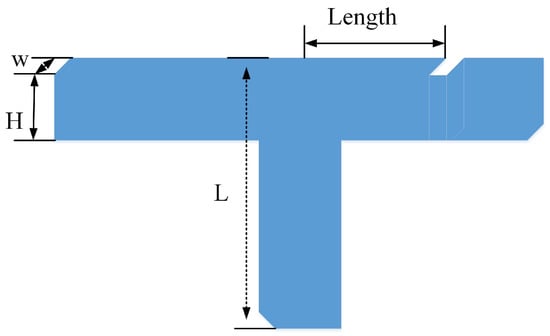
Figure 2. Parametric structure of the T-shaped waveguide antenna.

The design requirements of the T-shaped waveguide antenna are listed in Table 2.

Table 2. Design requirements of T-shaped waveguide antenna.

Frequency	1.0–10.0 GHz
Input Impedance	50 $\mathrm{\Omega }$
VSWR	≤2.0
Scan angle	$-180°\le \theta \le 180°$, $\phi =0°$

According to the design requirements of the antenna, the antenna design problem is converted to a COP as follows:

$$\begin{array}{c}\hfill \begin{array}{cc}min\hfill & -Gain,VSWR\hfill \\ st:\hfill & VSWR-2.0\le 0\hfill \\ & \mathit{X}=\left\{\mathit{x}\right|\mathit{l}\le \mathit{x}\le \mathit{u}\}\hfill \\ & \mathit{x}=[L,W,H,Length]\hfill \\ & \mathit{l}=[1.0,0.15,0.1,0.5],(unit:mm)\hfill \\ & \mathit{u}=[4.0,2.5,1.5,3.5]\hfill \end{array}\end{array}$$

(10)

where the voltage standing wave ratio (VSWR) and gain (which measures the effective radiated power of an antenna in a particular direction) of the antenna are considered as the objective function; $VSWR\le 2.0$ is a constrained function; $\mathit{x}$ is the solution vector; $\theta$ is the elevation angle with $10°$ increments over the range from $-180°$ to $180°$; and $\varphi$ is the azimuth angle with $0°$.

The evolved antenna is obtained by the proposed algorithm, and the optimum structure is $\mathit{x}$ = [L = 2.0 mm, W = 0.9 mm, H = 0.4 mm, $Length$ = 2.5148 mm]. The VSWR and gain results from the algorithms are shown in Figure 3 and Figure 4, respectively. We can observe that the evolved antenna satisfies the wideband antenna design requirements in Table 2. Through the wideband antenna design, the effectiveness of the proposed algorithm is verified further.

Figure 3. VSWR of the optimized of T-shaped waveguide antenna.

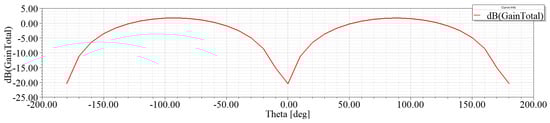
Figure 4. Gain of the optimized of T-shaped waveguide antenna.

A comparison of the total number of costly HFSS simulations required by DCMOEA-MLP and DCMOEA-NSGA-II for the T-shaped waveguide antenna design is presented in Table 3. The results demonstrate that DCMOEA-MLP requires significantly fewer simulations than DCMOEA-NSGA-II. Consequently, DCMOEA-MLP exhibits superior computational efficiency and performance in optimizing the T-shaped waveguide antenna.

Table 3. Comparison on the total number of expensive HFSS simulations for T-shaped waveguide antenna design.

Algorithm	DCMOEA-NSGA-II	DCMOEA-MLP
Number	1338	60,000

4.2. Example2: Microstrip Array Antenna Design

An array antenna consists of multiple antenna elements to transmit or receive radio waves. The array antenna can achieve good directionality with a narrow beam of radio waves. Hence, array antennas are usually widely studied in engineering. The microstrip array antenna is one of the simplest forms of array antennas, which are widely used in various applications because they offer good antenna performances and have a small size. In this paper, we will focus on designing an array antenna consisting of $3\times 3$ horn antenna elements. The distance between elements is $a1+length3$ in U direction, and $b1+length3$ in V direction. The horn antenna consists of a flaring metal waveguide shaped like a horn to direct radio waves in a beam. The layout of the rectangular horn antenna is shown in Figure 5. The rectangular horn antenna consists of a short length of rectangular metal tube closed at one end, flaring into an open-ended conical horn on the other end.

Figure 5. Parametric structure of the horn antenna element.

The requirements of the horn array antenna are listed in Table 4. According to the requirements of the horn array antenna, the antenna design problem is converted to a COP as follows:

$$\begin{array}{c}\hfill \begin{array}{cc}min\hfill & -Gain,S11\hfill \\ st:\hfill & S11+15.0\le 0\hfill \\ & \mathit{X}=\left\{\mathit{x}\right|\mathit{l}\le \mathit{x}\le \mathit{u}\}\hfill \\ & \mathit{x}=[a,b,length1,length2,a1,b1,length3]\hfill \\ & \mathit{l}=[3.0,1.5,0.5,15.0,12.5,7.5,0.5](unit:in)\hfill \\ & \mathit{u}=[6.0,2.6,2.0,40.0,18.5,11.5,5.5]\hfill \end{array}\end{array}$$

(11)

where gain and $S11$ (scattering parameter) of the antenna are considered as the objective function; $S11\le -$15 dB is a constrained function; $\mathit{x}$ is the solution vector; $\theta$ is the elevation angle with $5°$ increments over the range from $-50°$ to $50°$; and $\varphi$ is the azimuth angle with $90°$.

Table 4. Design requirements of horn array antenna.

Frequency	2.5–2.8 GHz
Input impedance	50 $\mathrm{\Omega }$
S11	≤−15 dB
Scan angle	$-50°\le \theta \le 50°$, $\phi =90°$

The optimum structure of the evolved horn array antenna by the proposed algorithm is $\mathit{x}=[a=4.7953in,b=2.1135in,$ $length1=1.2840in,length2=28.8241in,$ $a1=15.7362in,b1=9.3112in,$ $length3=1.8557in]$. The $S11$ and gain results are shown in Figure 6 and Figure 7, respectively. Through observing these results, the evolved horn array antenna satisfies the design requirement in Table 4. The effectiveness of the proposed algorithm in designing array antennas is verified further.

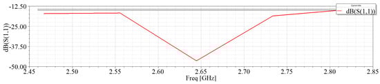
Figure 6. S11 of the optimized of horn array antenna.

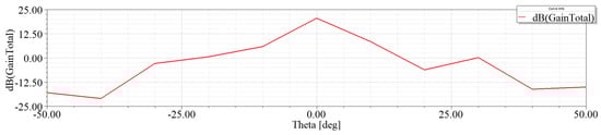
Figure 7. Gain of the optimized of horn array antenna.

To verify the effectiveness of the DCMOEA-MLP in reducing computationally expensive HFSS simulations for horn array antenna optimization, a comparative analysis of the number of HFSS simulations required by DCMOEA-MLP and DCMOEA-NSGA-II is conducted. Experimental results (see Table 5) further indicate that DCMOEA-MLP significantly outperforms DCMOEA-NSGA-II in minimizing the use of costly HFSS evaluations. Specifically, DCMOEA-NSGA-II required a total of 100,000 HFSS simulations, yet failed to converge to feasible solutions for the horn array antenna optimization problem.

Table 5. Comparison of the total number of expensive HFSS simulations for horn array antenna design.

Algorithm	DCMOEA-NSGA-II	DCMOEA-MLP
Number	12,659	100,000

5. Conclusions

This paper proposes a surrogate-assisted dynamic constrained multi-objective evolutionary algorithm framework for addressing expensive and highly constrained antenna optimization problems. An MLP surrogate model is employed to replace computationally expensive full-wave EM simulations, significantly reducing the computational burden of the optimization process. Moreover, a dynamic scaling-based constrained boundary strategy is introduced to enhance the algorithm’s efficiency in handling highly constrained problems. The effectiveness of the proposed approach has been validated through extensive experiments on constrained benchmark problems as well as two practical antenna design cases. Results demonstrate that the proposed framework achieves competitive performance in solving highly constrained problems under limited computational budgets. In future work, radiation characteristics such as beamwidth, sidelobe level, and directivity will be incorporated as both optimization objectives and constraints. The proposed algorithm will be applied to antenna design within the upper mid-band range (7–24 GHz) [36]. Furthermore, the optimization framework will be extended to include specific SAR and temperature as either objectives or constraints within the multi-objective formulation, thereby enabling explicit control over electromagnetic exposure in human–device interaction scenarios. Lastly, the development of a lightweight, embedded-compatible version of the surrogate model represents a promising direction for further investigation.

References

- Bazziand, A.; Chafii, M. On outage-based beamforming design for dual-functional radar-communication 6G systems. IEEE Trans. Wirel. Commun. 2023, 22, 5598–5612. [Google Scholar]
- Saunders, S.R.; Aragón-Zavala, A.A. Antennas and Propagation for Wireless Communication Systems; John Wiley & Sons: Hoboken, NJ, USA, 2024. [Google Scholar]
- Pietrenko-Dabrowska, A.; Koziel, S. Accelerated Parameter Tuning of Antenna Structures by Means of Response Features and Principal Directions. IEEE Trans. Antennas Propag. 2023, 23, 8987–8999. [Google Scholar] [CrossRef]
- Vodvarka, K.; Jurisic Bellotti, M.; Vucic, M. Design of Uniformly Excited Unequally Spaced Antenna Arrays by Using Nonlinear Optimization. IEEE Antennas Wirel. Propag. Lett. 2024, 23, 1463–1467. [Google Scholar] [CrossRef]
- Pu, S.; Dong, W.; Xu, Z.; Zeng, H.; Yang, G. Joint Optimization of Domino Subarray Tiling and Generalized Directivity Based on Iterative Convex Relaxation. IEEE Antennas Wirel. Propag. Lett. 2023, 23, 483–487. [Google Scholar] [CrossRef]
- Rahmat-Samii, Y.; Kovitz, J.M.; Rajagopalan, H. Nature-inspired optimization techniques in communication antenna designs. Proc. IEEE 2012, 100, 2132–2144. [Google Scholar] [CrossRef]
- Peng, F.; Chen, X. A General Optimization Method for Complex Requirements Antenna Based on Balanced Demotion MOEA. IEEE Trans. Antennas Propag. 2023, 71, 4663–4674. [Google Scholar] [CrossRef]
- Wolff, M.W.; Nanzer, J.A. Application of Pseudoweights in Antenna Array Optimization and Design. IEEE Antennas Wirel. Propag. Lett. 2024, 23, 1478–1482. [Google Scholar] [CrossRef]
- Jin, Y.; Wang, H.; Chugh, T.; Guo, D.; Miettinen, K. Data-Driven Evolutionary Optimization: An Overview and Case Studies. IEEE Trans. Evol. Comput. 2019, 23, 442–458. [Google Scholar] [CrossRef]
- Zhang, F.; Mei, Y.; Nguyen, S.; Zhang, M.; Tan, K.C. Surrogate-Assisted Evolutionary Multitask Genetic Programming for Dynamic Flexible Job Shop Scheduling. IEEE Trans. Evol. Comput. 2021, 25, 651–665. [Google Scholar] [CrossRef]
- Chugh, T.; Chakraborti, N.; Sindhya, K.; Jin, Y. A data-driven surrogate-assisted evolutionary algorithm applied to a many-objective blast furnace optimization problem. Mater. Manuf. Process. 2017, 32, 1172–1178. [Google Scholar] [CrossRef]
- Guo, D.; Wang, X.; Gao, K.; Jin, Y.; Ding, J.; Chai, T. Evolutionary Optimization of High-Dimensional Multiobjective and Many-Objective Expensive Problems Assisted by a Dropout Neural Network. IEEE Trans. Syst. Man Cybern. Syst. 2022, 52, 2084–2097. [Google Scholar] [CrossRef]
- Ghoni, R.; Dollah, M.; Sulaiman, A.; Ibrahim, F.M. Defect characterization based on eddy current technique: Technical review. Adv. Mech. Eng. 2014, 6, 182496. [Google Scholar] [CrossRef]
- D’Angelo, G.; Rampone, S. Feature extraction and soft computing methods for aerospace structure defect classification. Measurement 2016, 85, 192–209. [Google Scholar] [CrossRef]
- Yu, L.; Ren, C.; Meng, Z. A Surrogate-Assisted Differential Evolution with fitness-independent parameter adaptation for high-dimensional expensive optimization. Inf. Sci. 2024, 662, 120246. [Google Scholar] [CrossRef]
- Fu, K.; Cai, X.; Yuan, B.; Yang, Y.; Yao, X. An Efficient Surrogate Assisted Particle Swarm Optimization for Antenna Synthesis. IEEE Trans. Antennas Propag. 2022, 70, 4977–4984. [Google Scholar] [CrossRef]
- Yu, M.; Liang, J.; Zhao, K.; Wu, Z. An aRBF surrogate-assisted neighborhood field optimizer for expensive problems. Swarm Evol. Comput. 2022, 68, 100972. [Google Scholar] [CrossRef]
- Dong, J.; Li, Q.; Deng, L. Fast multi-objective optimization of multi-parameter antenna structures based on improved MOEA/D with surrogate-assisted model. AEU-Int. J. Electron. Commun. 2017, 72, 192–199. [Google Scholar] [CrossRef]
- Jiao, R.; Sun, Y.; Sun, J.; Jiang, Y.; Zeng, S. Antenna design using dynamic multi-objective evolutionary algorithm. IET Microwaves Antennas Propag. 2018, 12, 2065–2072. [Google Scholar] [CrossRef]
- Xu, Q.; Zeng, S.; Zhao, F.; Jiao, R.; Li, C. On Formulating and Designing Antenna Arrays by Evolutionary Algorithms. IEEE Trans. Antennas Propag. 2021, 69, 1118–1129. [Google Scholar] [CrossRef]
- Singh, P.; Rossi, M.; Couckuyt, I.; Deschrijver, D.; Rogier, H.; Dhaene, T. Constrained multi-objective antenna design optimization using surrogates. Int. J. Numer. Model. Electron. Netw. Devices Fields 2017, 30, e2248. [Google Scholar] [CrossRef]
- Mezura-Montes, E.; Coello, C.A.C. Constraint-handling in nature-inspired numerical optimization: Past, present and future. Swarm Evol. Comput. 2011, 1, 173–194. [Google Scholar] [CrossRef]
- Smitch, A.; Coit, D. Constraint-Handling Techniques-Penalty Functions. In Handbook of Evolutionary Computation (C 5.2); Oxford University Press: Bristol, UK, 1997. [Google Scholar]
- Deb, K. An efficient constraint handling method for genetic algorithms. Comput. Methods Appl. Mech. Eng. 2000, 186, 311–338. [Google Scholar] [CrossRef]
- Mallipeddi, R.; Suganthan, P.N. Ensemble of constraint handling techniques. IEEE Trans. Evol. Comput. 2010, 14, 561–579. [Google Scholar] [CrossRef]
- Xu, T.; He, J.; Shang, C. Helper and equivalent objectives: Efficient approach for constrained optimization. IEEE Trans. Cybern. 2020, 52, 240–251. [Google Scholar] [CrossRef] [PubMed]
- Zeng, S.; Jiao, R.; Li, C.; Li, X.; Alkasassbeh, J.S. A general framework of dynamic constrained multiobjective evolutionary algorithms for constrained optimization. IEEE Trans. Cybern. 2017, 47, 2678–2688. [Google Scholar] [CrossRef] [PubMed]
- Stein, M. Large sample properties of simulations using Latin hypercube sampling. Technometrics 1987, 29, 143–151. [Google Scholar] [CrossRef]
- Tian, J.; Tan, Y.; Zeng, J.; Sun, C.; Jin, Y. Multiobjective infill criterion driven Gaussian process-assisted particle swarm optimization of high-dimensional expensive problems. IEEE Trans. Evol. Comput. 2018, 23, 459–472. [Google Scholar] [CrossRef]
- Rahimi, A.; Recht, B. Random features for large-scale kernel machines. Adv. Neural Inf. Process. Syst. 2007, 20. [Google Scholar]
- Fabian, P.; Gael, V.; Alexandre, G.; Vincent, M. Scikit-learn: Machine Learning in Python. J. Mach. Learn. Res. 2011, 12, 2825–2830. [Google Scholar]
- Pratticò, D.; Laganà, F.; Oliva, G.; Fiorillo, A.S.; Pullano, S.A.; Calcagno, S.; Carlo, D.D.; Foresta, F.L. Integration of LSTM and U-Net models for monitoring electrical absorption with a system of sensors and electronic circuits. IEEE Trans. Instrum. Meas. 2025, 74, 2533311. [Google Scholar] [CrossRef]
- Liang, J.; Runarsson, T.P.; Mezura-Montes, E.; Clerc, M.; Deb, K. Problem definitions and evaluation criteria for the CEC 2006 special session on constrained real-parameter optimization. J. Appl. Mech. 2006, 41, 8–31. [Google Scholar]
- Zhang, Q.; Liu, W.; Tsang, E.; Virginas, B. Expensive multiobjective optimization by MOEA/D with Gaussian process model. IEEE Trans. Evol. Comput. 2010, 14, 456–474. [Google Scholar]
- Chugh, T.; Jin, Y.; Miettinen, K.; Hakanen, J.; Sindhya, K. A surrogate-assisted reference vector guided evolutionary algorithm for computationally expensive many-objective optimization. IEEE Trans. Evol. Comput. 2016, 22, 129–142. [Google Scholar]
- Bazzi, A.; Bomfin, R.; Mezzavilla, M.; Rangan, S.; Rappaport, T.; Chafii, M. Upper mid-band spectrum for 6G: Vision, opportunity and challenges. arXiv 2025, arXiv:2502.17914. [Google Scholar] [CrossRef]
Disclaimer/Publisher’s Note: The statements, opinions and data contained in all publications are solely those of the individual author(s) and contributor(s) and not of MDPI and/or the editor(s). MDPI and/or the editor(s) disclaim responsibility for any injury to people or property resulting from any ideas, methods, instructions or products referred to in the content. |
© 2025 by the authors. Licensee MDPI, Basel, Switzerland. This article is an open access article distributed under the terms and conditions of the Creative Commons Attribution (CC BY) license (https://creativecommons.org/licenses/by/4.0/).